
Optical Medieval Music Recognition Using Background Knowledge


Department for Artificial Intelligence and Knowledge Systems, University of Wuerzburg, D-97074 Wuerzburg, Germany
*
Author to whom correspondence should be addressed.
Algorithms 2022, 15(7), 221; https://0-doi-org.brum.beds.ac.uk/10.3390/a15070221
Submission received: 30 May 2022
/
Revised: 16 June 2022
/
Accepted: 19 June 2022
/
Published: 22 June 2022
(This article belongs to the Special Issue Machine Understanding of Music and Sound)
Abstract
:This paper deals with the effect of exploiting background knowledge for improving an OMR (Optical Music Recognition) deep learning pipeline for transcribing medieval, monophonic, handwritten music from the 12th–14th century, whose usage has been neglected in the literature. Various types of background knowledge about overlapping notes and text, clefs, graphical connections (neumes) and their implications on the position in staff of the notes were used and evaluated. Moreover, the effect of different encoder/decoder architectures and of different datasets for training a mixed model and for document-specific fine-tuning based on an extended OMR pipeline with an additional post-processing step were evaluated. The use of background models improves all metrics and in particular the melody accuracy rate (mAR), which is based on the insert, delete and replace operations necessary to convert the generated melody into the correct melody. When using a mixed model and evaluating on a different dataset, our best model achieves without fine-tuning and without post-processing a mAR of 90.4%, which is raised by nearly 30% to 93.2% mAR using background knowledge. With additional fine-tuning, the contribution of post-processing is even greater: the basic mAR of 90.5% is raised by more than 50% to 95.8% mAR.
1. Introduction
As most musical compositions in the western tradition have been written rather than recorded, the preservation and digitization of those musical documents by hand is time-consuming and often error-prone. Optical Music Recognition (OMR) is one of the key technologies to accelerate and simplify this task in an automatic way. Typically, an OMR system takes an image or manuscript of a musical composition and transforms its content encoded in some digital format such as MEI or MusicXML. Since the process of automatically recognizing musical notations is rather difficult, the usual OMR approach divides the problem in several sub-steps: (1) Preprocessing and deskewing, (2) staff line detection, (3) symbol detection and (4) finally the reconstruction and generation of the target encoding.
On modern documents, the OMR process already obtains very good results. However, on historical handwritten documents the performance is much worse and requires expert knowledge in some cases. This is due to the fact that those documents are much more heterogeneous, often differ in their quality, and are affected from various degradations such as bleed-through. Furthermore, the notation of early music documents had been developed and thus changed several times, requiring different solutions. The main contribution is formalizing parts of this expert knowledge and incorporating it into a post-processing pipeline to improve the symbol detection task.
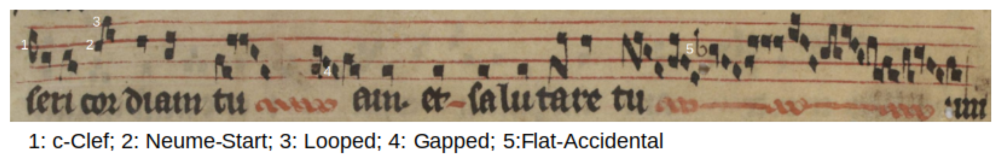
This work focuses on symbol detection and segmentation tasks and deals with manuscripts written in square notation, an early medieval notation, which was used from the 11th–12th century onwards. A staff usually contains four lines and three spaces and in most cases a clef marker at the start. Sample images of such manuscripts can be seen in Section 3.
The extraction of the symbols is addressed as a segmentation task. For this, a Fully Convolutional Network (FCN), which predicts pixel-based locations of music symbols, is used. Further post-processing steps extract the actual positions and symbol types. Furthermore, the pitch of the symbols can be derived from the position on the staff of the symbol relative to the position of the clef on the staff and other pitch alterations. The fundamental architecture used for this task resembles the U-Net [1] structure. The U-Net structure is symmetric and consists of two major parts: an encoder part consisting of general convolutions and a decoder part consisting of transposed convolutions (upsampling). For the encoder part, several architectures, which are often used for image classification tasks, are evaluated. The decoder part was expanded so that it fits the architecture of the encoder part. Furthermore, a post-processing pipeline is introduced that aims to improve the symbol recognition using background knowledge.
Background knowledge comprises implicit knowledge used by human experts to decide ambiguous situations in addition to the direct notation. The knowledge covers various sources, e.g., conventions, melodic knowledge, constraints based on the notation, knowledge about the scan process, and may be general- or source-document-specific, respectively. It ranges from quite simple conventions, e.g., every text syllable needs at least one note over context dependent decisions, e.g., translucent notes in a scan with a different appearance on each page, to rather complex knowledge, e.g., about typical melodies. In this work, a post-processing pipeline uses background knowledge to correct wrong clefs and symbols, graphical connections and wrong note pitches caused by an incorrect staff line assignment.
The rest of this paper is structured as follows: First, the related work for OMR on historical manuscripts, focusing on the music symbol segmentation task, is presented. Afterwards, the used datasets are introduced, followed by the description of the proposed workflow and the post-processing pipeline. Finally, the results are presented and discussed and the paper is concluded by giving an outlook for future work.
2. Related Work
The use of Deep Neural Network techniques has reported outstanding results in many areas related to computer vision, including OMR. Pacha et al. treated this problem as an object detection task [2,3]. Their pipeline uses an existing deep convolutional neural network for object detection such as Faster R-CNN [4] or YOLO [5] and yields the bounding boxes of all detected objects along with their most likely class. Their dataset consists of 60 fully annotated pages from the 16th–18th century with 32 different classes written in mensural notation. Typically, for object detection methods, the mean Average Precision (mAP) was used as the evaluation metric. A bounding box is considered as correctly detected if it overlaps 60% of the ground-truth box. Their proposed algorithm yielded 66% mAP. Further observation showed that especially small objects such as dots or rests posed a significant challenge to the network.
Alternatively, the challenge can be approached as a sequence-to-sequence task [6,7,8,9]. Van der Wel et al. [6] used a Convolutional Sequence-to-Sequence model to segment musical symbols. A common problem for segmentation tasks is the lack of ground truth. Here, the model is trained with the Connectionist Temporal Classification (CTC) loss function [10], which has the advantage that it is not necessary to provide information about the location of the symbols in the image; just pairs of input scores and their corresponding transcripts are enough. The model was trained on user generated scores from the MuseScore Sheet Music Archive (Musescore: https://musescore.org/, accessed on 30 May 2022) to predict a sequence of pitches and durations. In total, the dataset consisted of about 17,000 MusicXML scores, of which 60% were used for training. Using data augmentation, a pitch and duration accuracy of 81% and 94% was achieved, respectively. The note accuracy, where both pitch and duration are correctly predicted, was 80%.
Calvo-Zaragoza et al. [11] used Convolutional Neural Networks for automatic document processing of historical music images. Similar to our task, the corpus used for training and evaluation was rather small, consisting of 10 pages of the Salzinnes Antiphonal (https://cantus.simssa.ca/manuscript/133/, accessed on 30 May 2022) and 10 pages of the Einsiedeln (http://www.e-codices.unifr.ch/en/sbe/0611/, accessed on 30 May 2022). Both of them are also written in square notation. The task was addressed as a classification task, where each pixel in the image was assigned one of four selected classes: text, symbol, staff line or background. The input to the network were small patches extracted from the pages centered at the point of interest. Each pixel was evaluated with the -metric for the four classes. This yielded an average -score of around 90%, while the music symbols’ specific -score was about 87.46%.
Similar to that, Wick et al. [12] also considered this as a segmentation task. A FCN was used to detect staff lines and symbols in documents. The staff line detection achieved a -score of over 99%. For the symbol detection task, they achieved an -score of over 96% if the type is ignored. By using a sequence-to-sequence metric, the so-called diplomatic symbol accuracy rate (dSAR) [12] (see Section 8.2), they reached an accuracy of about 87%. A similar approach can be observed in [13]. Other approaches use handcrafted features or heuristics for the symbol recognition task, such as in [14] using Kalman filters or [15,16] using projections.
To the best of our knowledge, we are not aware of any other publications that attempt to incorporate background knowledge about medieval documents in order to improve the recognition rate.
3. Datasets
A typical staff picture can be observed in Figure 1. For training and evaluation, a combination of different manuscripts is used. One of the larger one was presented in [12] (Available under: https://github.com/OMMR4all/datasets, accessed on 30 May 2022). It consists of 49 pages of the manuscript “Graduel de Nevers”, which was published in the 12th century. A total of six different classes are stored in the dataset. These include C-clef, F-clef, Flat-accidentals, and three different types of Note Components (NC), being either a neume start, a gapped or looped NC.
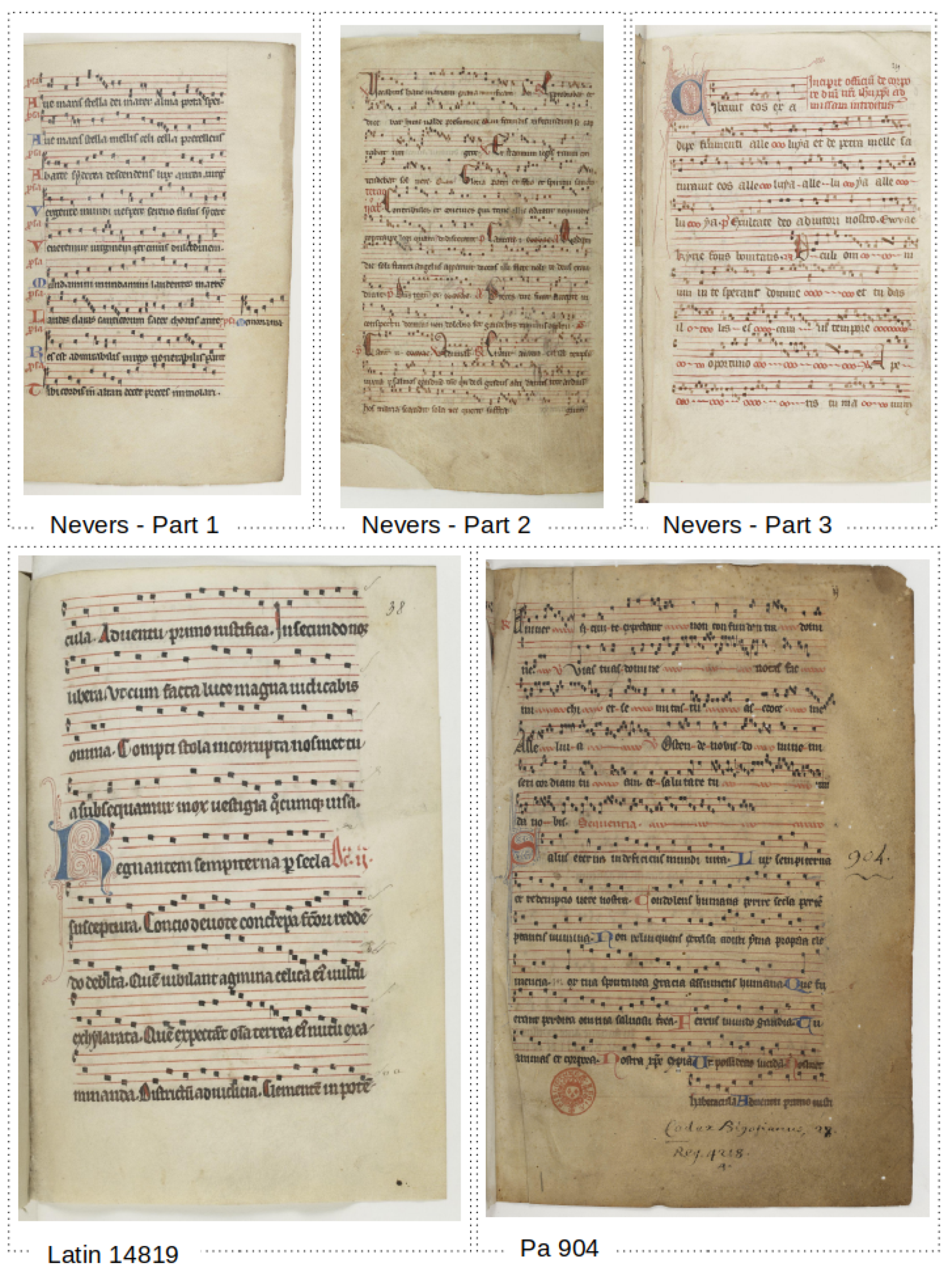
This dataset is divided into three parts with varying layouts and difficulty, based on human intuition [12]. The first part contains scans with the best notation quality available. The symbols are visually more distinct and separated than in the other parts. Part 2 is the most difficult one, since the notation of the musical components is more dense and the contrast of the staff lines is worse, compared to part 1. Part 3 is similar to part 1, but consists of wavy staff lines and some more challenging musical components.
The “Latin14819” dataset consists of 182 pages of the manuscript “Latin14819” (Available under: https://gallica.bnf.fr/ark:/12148/btv1b84229841/, accessed on 30 May 2022), which was published between the 12th–14th century. The notation layout of the available pages is similar to part 1 of “Graduel de Nevers”. The symbols and lines are distinct, the contrast of the musical components is good and the symbols are often separated by space, which reduces the danger of confusion.
The Pa904 dataset consists of 20 pages of the manuscript “Pa904” (Available under: https://gallica.bnf.fr/ark:/12148/btv1b84324657, accessed on 30 May 2022). It was published between the 12th–13th century. The symbols are much denser here, which makes segmentation more difficult. The ratio of faded to non-faded symbols is also greater than in the other datasets. An overview of the datasets is given in Table 1, an example page for each dataset is shown in Figure 2.
4. Workflow
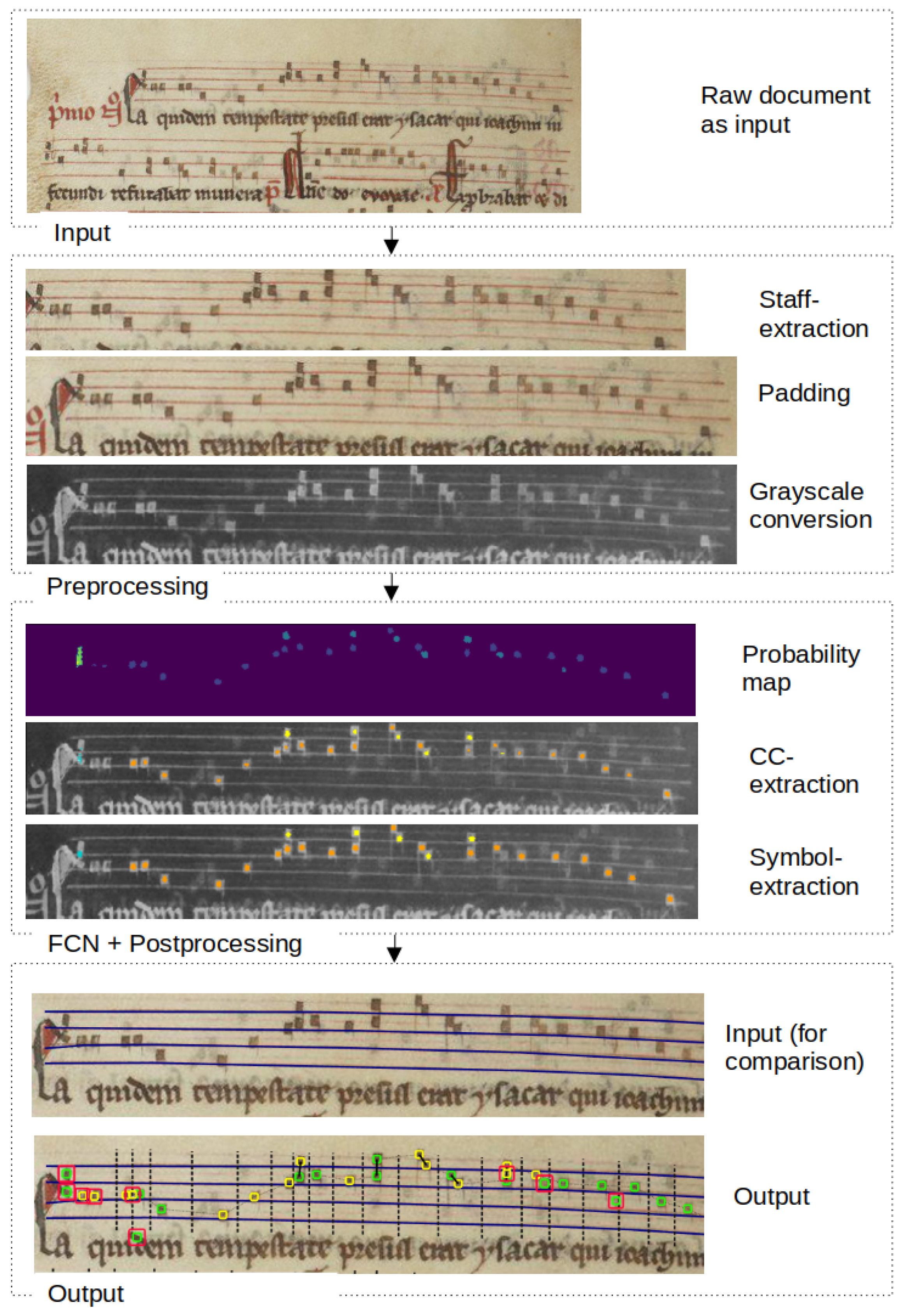
Figure 3 illustrates the general workflow. As depicted, the inputs to the general workflow are the raw documents. Since the scale of the systems can be different for each page, the staff line distance , which is the average distance from one staff line to the next staff line, is calculated as a preprocessing step in order to normalize the raw input pages to an equal scale. Additionally, the inputs are converted to grayscale color space. Since the input of the proposed symbol detection algorithm is based on staffs, the next step is the extraction of each individual staff image. This can be conducted with a FCN as shown in [12] with an automatic detection rate of the staff lines in historical documents of of all staff lines and detection of the correct length with a -Score. As this work focuses on the symbol detection part of the OMR pipeline, the encoded system lines of the dataset are used directly instead of the detected ones, even though the detection rates are very good, as shown in [12].
Furthermore, the bounding box of the extracted staff is calculated and extended by the addition of a margin of one . Since the position of clefs is often at the start of a staff, the bounds of the bounding box are therefore extended to the left by an additional . Afterwards, the calculated bounding boxes are extracted and scaled to a fixed height of 80 pixels, in order to normalize the resolution of the symbols. The extracted images are optionally augmented and are fed to the FCN. The augmentations used for training are rotate, shift, shear and zoom transformations on the input images. The FCN trained to discriminate between music symbols and background pixels predicts a heat map. Each pixel is then labeled to the class with the highest probability. Afterwards, CCs are extracted and classified according to the label with the highest amount of pixels.
The FCN is trained on Ground Truth containing the human-annotated music symbols, which are drawn as a circle with a radius of of the average space between two lines of the staff and using the negative-loss-likelihood as a loss function. The radius is calculated for every staff independently. The center of the extracted CCs determines the position of the symbols. The position in line assignment (PIS) (including the auxiliary lines) of the symbols is based solely on the distance to the closest staff line and space. Even though the notes are visually closer to space, they are likely to intersect the area of the line. Therefore, the area of the non-auxiliary lines is extended to take this fact into account. Finally, the pitch is calculated based on the position of the symbols on the staff, the previous clef and other alterations.
5. Post-Processing Pipeline
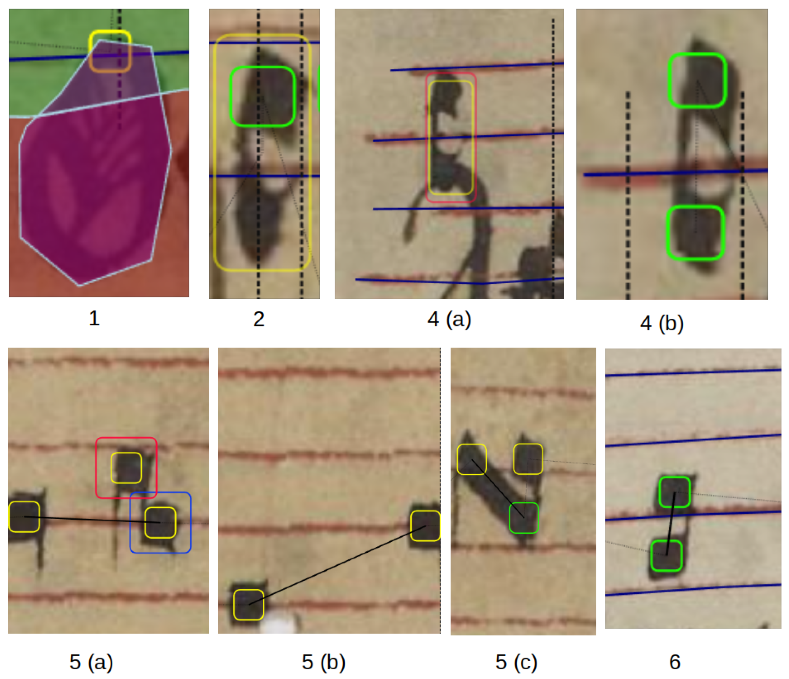
In this section, the post-processing pipeline is introduced. This pipeline uses the symbols extracted from the probability map. Using the probability map, each pixel in the image is labeled to the symbol class with the highest probability (excluding background). This results in a symbol label map. Next, the system decides whether there is background or a symbol. This is conducted in a separate step where the pixels are suppressed when the background class is above a certain threshold (). The new filtered symbol label map is then used by a connected component analysis [17] to extract the symbols. As mentioned previously, the symbols are segmented using two different thresholds for : To extract the baseline symbols, the threshold is set to . To extract additional symbols, the threshold is set to and filtered afterwards using the baseline symbols such that only the additional “uncertain” symbols remain. There are many False Positives (FP) in these uncertain symbols, but also False Negatives (FN) symbols that were not segmented with the lower threshold. These additional symbols are used in the post-processing steps to improve the recognition rate with the usage of background knowledge. In Figure 4, examples of issues the system tries to fix with the post-processing pipeline are shown. Our post-processing steps are described below:
- 1.
- Correct symbols in wrong layout blocks: Sometimes FP are recognized inside incorrect layout blocks, such as drop capitals, lyrics, or paragraphs. Such symbols are removed from the baseline symbols and the uncertain symbols if they are inside drop capitals. If symbols appear in text regions, they are also removed if the vertical distance to the nearest staff line is greater than a constant .
- 2.
- Overlapping symbols: In this post-processing step, symbols that overlap are removed. Since only the centers are recognized by our symbol recognition, the outline for each symbol depending on is calculated. Due to the fact that notes appear as squares in the original documents, a box around the center with a width and height of can be drawn. Because clefs are bigger and also differ in height and width, this value is modified slightly. For C-Clefs, a box with a width of and a height of is drawn. For F-Clefs, a width of and a height of is used. If a clef overlaps a symbol, the clef is prioritized and the symbol is removed. If two symbols overlap each other, and they have the same PIS, one of them is removed.
- 3.
- Position in staff of clefs: In the datasets, all clefs appear to be only on top of a staff line and not in between. If the algorithm has detected that the PIS of a clef is in between two staff lines, then the clef is moved to the closest staff line.
- 4.
- Missing clefs in the beginning of a staff line: Normally, a staff always begins with a clef. If this is not the case, the system tries to fix it:
- (a)
- Additional symbols: If no clef is recognized by the algorithm at the beginning, it is checked if a clef has been recognized in the uncertain symbols. If so, this clef is added to the baseline symbols.
- (b)
- Merging symbols: The C and F-clef consists of two boxes. It can happen that a clef is mistaken for two notes. Therefore, two vertically stacked symbols that appear at the beginning of a staff are replaced by a clef. This is only performed when the position of the two symbols is right at the beginning, which means that the symbols are no more than away from the start of the staff lines.
- (c)
- Prior knowledge: If the above steps did not help, a clef is then inserted at the beginning, based on the clefs of previous staves. This can lead to FP for the segmentation task, even if a clef has to be inserted at this position, because the exact center position can only be guessed. Nevertheless, it has a positive effect on the recognized melody.
- 5.
- Looped graphical connection: This post-processing step aims to fix errors in the graphical connection, i.e., fixes between neume start, gapped and looped classes.
- (a)
- Additional symbols: The algorithm looks for consecutive notes that have a graphical connection between them. If the horizontal distance between these symbols is larger than , it is corrected. If there is an uncertain symbol in between, it is added to the baseline symbols.
- (b)
- Replace class: If there is none, the class of the symbol is changed from “looped” to “neume start”
- (c)
- Stacked symbols: In addition to that, the system also recognizes stacked symbols. If the horizontal distance between them is less than , a graphical connection is inserted between them.
- 6.
- PIS of stacked notes: The PIS of the notes is often distorted due to the limited space on the staffs, because the author of the handwritten manuscripts wanted to maintain some structural characteristic of some neumes (e.g., in Podatus or Clivis neumes (https://music-encoding.org/guidelines/v3/content/neumes.html), accessed on 30 May 2022). However, due to the lack of space and to preserve the characteristics, the notes cannot be placed directly on the staff where they should be, but are slightly shifted. Since the system uses the distance of the symbols to the staff lines and the space to calculate the position in the staff lines (PIS), this shift can lead to FP. The system corrects the PIS in borderline cases based on the confidence of the PIS algorithm for the notes of the respective neumes.
6. Architecture
As already mentioned, the pipeline takes advantage of the U-Net [1] architecture to segment the symbols from images. The U-Net is symmetric and consists of two parts: (i) The encoder (contracting path [1]), which is used to encode the input image into the feature representation at multiple different levels and (ii) the decoder, which projects the context information features [1] (expansive path) learned by the encoder onto the pixel space. For our experiments, several U-Net architectures were evaluated and compared. Details of the architectures can be found in the cited papers of Table 2. Two of the architectures that have been examined were already available as a complete U-Net with both the encoder and decoder part (i.e., FCN, U-Net). For the other architectures (MobileNet, ResNet, EfficientNet with different scaling factors: Eff-b1, Eff-b3, Eff-b5 and Eff-b7), only the encoder part was used, as these were originally designed for classification tasks. The decoder part was added to these architectures. The decoder part consists of a bridge block and upsample blocks. The bridge block consists of convolutional layers with 256 kernels with a size of 3 × 3. The number of upsamble blocks depends on the number of downsample blocks of the encoder. Each upsample block has two convolutional layers. The first upsample block consists of two layers with 256 kernels with a size of 3 × 3, each. The number of kernels is halved with each additional upsample block. In addition to that, skip-connections between the upsample blocks and the downsample blocks were added. Finally, a convolutional layer is added, which converts the output nodes at each position into 9 (8 classes + background) target probabilities at each pixel position of the image.
7. Layout Analysis
Since the symbol post-processing pipeline partially uses the layout, e.g., drop capitals or lyric regions of a page to correct symbols, this section briefly presents the layout analysis of the system. The aim of the layout analysis is to split the page into music regions and text regions. Text regions can be further split into lyric, paragraph and drop capitals. However, this is not mandatory. Figure 5 shows an example of such a layout recognition. The pipeline consists of two simple steps and uses the encoded staff lines of the dataset:
- 1.
- Music-Lyric: The bounding box for each encoded stave on a page is calculated and is padded with on the top and bottom side of the box. These are marked as music regions. Regions that lie between two music regions are marked as lyric regions. Since the bottom lyric line is not between two music regions, it is added separately. To do this, the average distance between two music regions (staffs) is calculated and afterwards used to determine the lowest music region.
- 2.
- Drop-Capital: Drop capitals (compare Figure 5) often overlap music regions, so these must be recognized separately. The pipeline uses a Mask-RCNN [21] with a ResNet-50 [19] encoder to detect drop capitals on the page.
- (a)
- Training: Since only limited data are available, the weights of the model trained on the COCO dataset [22] is used to fine-tune the model. For training, only horizontal flip augmentations are used. The network is then fine-tuned on the “Latin 14819” dataset. A total of 320 instances of drop capitals are included there. The model is trained with positive (images with drop capitals) and negative (images without drop capitals) examples. Inputs are the raw documents. SGD was used as the optimizer, with hyperparameters of learning rate = 0.005, momentum = 0.9 and weight decay = 0.0005.
- (b)
- Prediction: The raw documents are the input. A threshold of 0.5 is applied to the output of the model. Next, the output is used to calculate the concave hulls of the drop capitals on the document. If hulls overlap, all but one are removed and only the one with the smallest area is kept.
- (c)
- Qualitative Evaluation: A qualitative analysis on the Pa904 dataset was conducted. A total of 43 drop capitals were available on the pages. These could be subdivided into large, ornated ones and smaller ones, which still clearly protrude into the music regions. Afterwards, the recognized drop capitals were counted. It should be noted that the algorithm rarely recognized holes or inkblots as initials. These errors were ignored because the system only uses the drop capitals for the post-processing pipeline anyway and they do not cause errors for the symbol detection task. Results from the drop capital detection can be taken from Table 3. The error analysis showed that no FPs, such as neumes, were detected. Further experiments demonstrated similar results on other datasets without further fine-tuning. This is important because otherwise errors could be induced by the post-processing pipeline.
8. Results
In this section, the setting for the performed experiments is described, as well as their interpretation and the experimental conclusions that can be drawn. First, an overview of the experiments is presented, for which the results in this chapter are reported:
- 1.
- Evaluation of different encoder/decoder architectures within our complete OMR pipeline with data from the same dataset as the training data by a 5-fold cross validation (i.e., 80% of the data used for training, the remaining 20% for evaluation) with a large dataset (Nevers Part 1–3 + Latin 14,819 with 50,607 symbols; compare Table 1 (Table 4).
For the following evaluations, the simple baseline architecture (FCN) and the most promising architecture (Eff-b3) were used.
- 2.
- Evaluation of the OMR pipeline similar to experiment 1 on a smaller dataset (Nevers Part 1–3 with 15,845 symbols) with 5-fold cross validation, repeating an evaluation from the literature (Table 5);
- 3.
- Evaluation of the OMR pipeline on a different, challenging dataset (Pa904 with 9025 symbols on 20 pages) as a real-world use case:
- (a)
- With pretrained mixed model and document specific fine-tuning: Starting with the mixed model of experiment 1 and using 16 pages of the dataset for fine-tuning while evaluating on the remaining 4 pages (5-fold cross validation; Table 6)
- (b)
- With document specific training without a pretrained model: Using solely the Pa904 dataset for training and evaluation in a 5-fold cross validation similar to experiment 1. Here 4 architectures (FCN, U-Net, Eff-b3, Eff-b7; Table 6) are compared;
- (c)
- With a mixed model without fine-tuning: Using the mixed model of experiment 1 and evaluation of the 20 pages of the dataset Pa904 (Table 7).
- (4)
- Evaluation how effective the different parts of post-processing pipeline are for the mixed model with and without fine-tuning on the Pa904 dataset (Table 8);
- (5)
- Evaluation of the frequency of remaining error types with and without post-processing on the Pa904 dataset using the mixed model with fine-tuning (Table 9).
8.1. Metrics
It is common to evaluate the performance of the symbol detection rate of musical documents in a sequence-to-sequence manner, as can be observed in [12]. Therefore, the three main metrics used for evaluation are the diplomatic accuracy rate (dSAR), the harmonic symbol accuracy rate (hSAR) and the melody symbol accuracy rate (mAR). The normalized edit distance is used to compute those metrics: The algorithm is counting each insert, delete, and replace operation necessary to convert the output into the Ground Truth as one error and afterwards normalizes the total errors by the maximum length of the two sequences. Next, dSAR, hSAR and mAR is the corresponding accuracy rate by calculating , where is the respective normalized error rate of the sequence using the edit distance (dSER, hSER or mER). The only difference is how the sequences are calculated from the predicted symbols:
- dSAR: The diplomatic transcription compares the staff position and types of notes and clefs and their order; however, the actual horizontal position is ignored [12];
- hSAR: Similar to dSAR, but only evaluates the correctness of the harmonic properties, by ignoring the graphical connections of all note components (NC). [12];
- mAR: Evaluates the melody sequence. The melody sequence is generated from the predicted symbols by calculating the pitch for each note symbol.
The melody metric is quite harsh, but realistic. For example, in the Corpus Monodicum (https://corpus-monodicum.de, accessed 30 May 2022) project the transcription takes place with an editor [23] at pitch level. For a complete automatic transcription with later post-correction in this editor, this metric comes closest to the amount of corrections that are needed.
Additionally to these sequence metrics, three additional metrics are evaluated:
- Symbol detection accuracy: A predicted symbol is counted as correctly detected (TP) if the distance to its respective ground truth symbol is less than 5 px.
- Type accuracy: Only TP pairs are considered. Here, the correctness of the predicted graphical connection is evaluated.
- Position in staff accuracy: Only TP pairs are considered as well. Here, the correctness of the predicted position in staff is evaluated.
These three metrics are further subdivided in , and to respectively consider all symbols, only the notes or only the clefs.
8.2. Preliminary Experiments
All preliminary experiments were carried out using 5-fold cross validation, which splits each dataset into five smaller slices. Four slices are used for training and the remaining part is used for evaluating the algorithm. Since several datasets are used, each dataset is split individually into five folds and afterwards the corresponding folds of each part are merged to generate the training and the test set, in order to include every single dataset in a fair manner.
Table 4 shows the performance of the different network architectures. In this experiment, the weights are initialized with the pretrained weights from the ImageNet [24] dataset, if possible. All models were trained for a maximum of 30,000 steps, and a learning rate of 1 × 10 was chosen. Adam [25] is used as the optimizer. The upper block shows the results when no post-processing is used. The lower block display the results with the proposed post-processing steps. As a result of using a post-processing pipeline, the overall accuracy of each evaluated model improves on most metrics. Since our post-processing is also correcting clefs, the melody metric improved the most from 84.6% to 89.2% for the FCN architecture. Slightly poorer results can be observed for the “type” section. This can be explained by the fact that more symbols are detected with the post-processing pipeline. Hereby, symbols can be inserted, which have the correct position in the staff in most cases but also can have, e.g., the wrong note connection type. For calculating the correct melody, this is less important.
Moreover, in comparison to the baseline model (FCN), the usage of more advanced encoders yielded improved results, as well. Here, the model with the Eff-b5 encoder achieved the best accuracy with a mAR of 95.3%. By using larger encoders for the model, the post-processing effect is lower when enough training data are available.
The experiment from [12] is repeated to observe exactly how big the impact is of the post-processing using background knowledge. The experiment was run with and without the post-processing pipeline. Results are presented in Table 5. As in [12], the training and evaluation took place only on the Nevers datasets. No pretraining was used. The post-processing pipeline improved the dSAR by about 1%. The melody accuracy rate has improved by 8%. Using more advanced encoders, the mAR could further be improved by about 3%. This also shows that the post-processing is very robust and can be applied to other datasets as well.
8.3. Document-Specific Fine-Tuning
The Pa904 dataset was used for training and evaluation in this experiment. Each fold was trained on 16 pages. Evaluations were carried out on four pages each. In this experiment, the weights of the mixed model from the experiment in Table 4 were optionally used as a starting point for the document specific fine-tuning. This experiment reflects a real live scenario as closely as possible, in which only a few pages, if any, are available for training.
The results of the experiment can be observed in the Table 6. In general, it can be observed that both pretraining and post-processing improves the recognition rate of the symbol detection task. With the EfficientNet-b3 [20] encoder, the highest accuracy with a melody accuracy of 95.8% was achieved. It is noticeable that the post-processing improves the melody accuracy significantly, especially in simpler architectures such as the FCN. Here, the accuracy improves from 84.3% to 91.3%. The reason is that the simple encoders make more mistakes, and so there is a greater basis for improvement. Above all, wrong or missing clefs lead to the wrong segmentation of a complete sequence. A substantial improvement can also be observed in the more complex architectures.
8.4. Mixed Model Training without Fine-Tuning
This experiment evaluates the performance of an existing model when applied to new datasets. For this purpose, training was carried out on all datasets (compare the experiment in Table 4) except for the Pa904 and was subsequently evaluated exclusively on the Pa904 dataset. Results of this experiment can be observed in the Table 7. Interestingly, the mAR value is comparable to the model, which was trained exclusively on the Pa904 dataset. This shows that the models generalize very well and can be easily applied to new datasets. The highest accuracy without post-processing of the system was achieved with the Eff-b3 encoder with a mAR of 90.4%. By adding the post-processing pipeline, a mAR of 93.2% was achieved, which is 2.5% less than using document specific fine-tuning (see above).
8.5. Evaluation of the Contribution of the Different Post-Processing Steps
The post-processing steps were evaluated on the Pa904 dataset. In addition, two models were compared with each other. On the one hand, the “fine-tuned” model, derived from Table 6, has been trained on all datasets (except Pa904) and is subsequently fine-tuned and evaluated on the Pa904 dataset. On the other hand, the “mixed-train” model from Table 7 is only evaluated on the Pa904 dataset, but is not trained on it. In Table 8, the influence on the mAR of the individual post-processing steps can be observed.
Steps one through three of the post-processing pipeline have only a small direct effect on the accuracy of the fine-tuned model, probably because document-specific fine-tuning helps the model to avoid very obvious mistakes, such as detecting symbols in text. This can also be observed in the mixed model, where such errors occur more frequently and can therefore be corrected through post-processing. Nevertheless, it should also be noted here that the fact that pretraining was conducted on a relatively large dataset. This allowed both models to generalize well to separate music symbols from text. We assume that pretraining with a smaller dataset would have resulted in more errors and therefore also a greater impact of those post-processing steps. It should also be noted that those post-processing steps also indirectly help to avoid errors, as, in addition to the baseline symbols, the unsafe symbols are also filtered and therefore not incorrectly used for a post-correction. Step six has the highest positive effect, which makes sense since the dataset has a lot of vertically stacked neumes, whereby the PIS of the symbols is often difficult to recognize. Step four also has a great impact, because correcting a clef can avoid many consequential errors. Step 5 has a similarly large improvement as step 4.
8.6. Error Analysis
The error distribution of the best performing “FCN” and “Eff-b3” model of the Pa 904 dataset is listed in Table 9. Both the error rate with and without post-processing is specified.
The edit distance was used to count the number of insertions, deletions and replacements to obtain the Ground Truth sequence. Replacements are counted as one insertion and one deletion. Therefore, correctly segmented symbols, that were predicted with a wrong type (e.g., instead of a c-clef, an f-clef), are counted as two errors (FN and FP). In general, more errors are caused by missing symbols rather than by the detection of additional symbols. This is the case for the models without post-processing as well as for those with post-processing. The post-processing pipeline balances the ratio between FN and FP, but is still in favor of FN.
Missing notes are one of the main errors of the symbol recognition. This was expected, since some of the documents are heavily affected by bleed-through noise. Because the contrast between the background and the symbols is sometimes too weak, this effect is intensified. In addition to that, symbols can protrude the text, often overlapping them, which means that they can only be recognized with the usage of context knowledge. After that, the most probable errors were wrongly predicted PIS of symbols with a relative amount of 24.5% (absolute 0.63%) in total (FP and FN). This is reasonable, because the decision if a note is, for example, on a staff line or between two lines can often only be decided based on context. Especially with single note neumes, it is difficult to correct PIS errors. Some first experiments were conducted using a simple language model with transitional probabilities of n-gram sequence pitches of the notes to correct those errors. However, we did not manage to incorporate this knowledge with a positive effect to the mAR, since it caused about the same number of errors that we were able to correct with it.
Without post-processing, clefs were the third-largest source of error on average, with an error rate of about 0.12%. This is still high, considering that clefs usually occur at most 1–2 times per line. Using post-processing, the error-rate decreases by about 25%. That was also to be expected, since a missing clef, especially those at the beginning, can be corrected relatively well with background knowledge. Altogether, errors concerning accidentals occur the least, which is not surprising since they only occur very rarely. That is also the reason why additional accidentals are not recognized, since the network has to be very confident to segment an accidental.
With the different encoder architectures, two things in particular could be observed: The more complex architectures recognize symbols better with a sufficient amount of training. Additionally, a finer localization of the note components could be observed when using these networks. This resulted in less PIS errors, since a poor localization of symbols sharing roughly the same horizontal position (this can, for example, be observed in a Podatus neume) can result in a sequence error. Moreover, reading order errors happen less, and are mainly caused by stacked NCs (e.g., a so-called PES or Scandicus neume), in which, e.g., the upper note is sung first because of a poor localization segmentation, but should in reality be sung later.
Since it is very important to recognize the clef correctly because wrong or unrecognized clefs cause subsequent errors, these errors were examined more closely. Without post-processing, one-third to one-fourth of all clef errors were missing clefs in the beginning of a staff line. In most cases, the clefs are located close to the text, whereby it is missed or recognized as one symbol. Clef errors that can be attributed to drop capitals, as these are close to each other, amount to about 10%. That seems logical, since a clef often occurs after a drop capital and can cause errors as a result. The second most common mistakes are wrong symbol types in the staff. Here, the most common cause is that a clef is mistaken as two symbols. Using the post-processing pipeline, the error rate of those errors can be reduced by quite a large margin. In particular, clefs that are missing at the beginning or are recognized as symbols can be corrected very well. Clefs in the middle of a staff, on the other hand, are quite difficult to correct.
In Table 10, a break-down of the missing and additional symbols is given, which amounts for 28.8% and 15.1% of the errors, respectively. Most errors related to both FP and FN are due to text proximity. Certain text errors are treated by the post-processing pipeline. In some cases, however, errors can only be corrected, if at all, with additional expert knowledge. At such points, the correction through background knowledge fails. (e.g., does a square belong to the text (i-dot) or is it a single note neume). The second most common error are horizontally adjacent symbols. We assume that this error is generated by a combination of the selected threshold value and the connected component analysis. With a perfectly tuned threshold, this error would presumably disappear. The same applies to symbols which are vertically close together. Faded symbols and rare symbols are also responsible for a big part of the errors. Correcting such an error would require either more context (e.g., syllables) or background knowledge of common melodies in order to know if a note is missing or not.
9. Conclusions
In this paper, we demonstrated the benefits of using background knowledge in combination with fully convolutional neural networks to tackle the automatic segmentation of symbols in historical musical documents. The following types of background knowledge were applied and evaluated: Adjust symbols in wrong layout blocks (drop capitals, lyrics and paragraphs), remove overlapping symbols, move clefs always on top of a staffline and not in between, add missing clefs in the beginning of a staff line, correct looped graphical connections, and change the position in the staff of stacked notes in borderline cases. Various architectures and datasets for an OMR pipeline were investigated and in all settings, the use of background knowledge increased the melody rate (mAR) by around 30% to 50%. In the best experiment, using an EfficientNet-b3 encoder with a mixed model and document specific fine-tuning, the background knowledge improves the mAR on the challenging Pa904 dataset from 90.5% to 95.8%. Compared to the previous works [12], the proposed method increased the dSAR metric on the “Graduel de Nevers” dataset by around 30%. Improvements are primarily achieved by recognizing more symbols and the post-processing pipeline, but also because the horizontal location of the networks is more accurate, which results in fewer sequence errors. An error analysis demonstrated that the main source of remaining errors are missing symbols and the predicted staff positions of the symbols indicated targets for further improvements. In conclusion, the post-processing has greatly improved the accuracy and is also very robust. Nevertheless, the post-processing still has a lot of potential for further improvements. Promising approaches will decide whether a note is translucent or not based on local context, in order to use rules about conventions over neumes and to use full or partial transcriptions from similar songs, if available. Another topic is the adaption of background knowledge to different types of manuscripts and notation styles. An ambitious goal is to add a step in the post-processing pipeline that incorporates a language model with knowledge of the most common melodies and transition probabilities between notes in order to correct further errors. This would even allow us to tackle previously uncorrectable errors, e.g., missing symbols caused by noise, and also to refine the existing post-processing steps with further background knowledge. Finally, such knowledge could be used not only to correct the automatic transcription but also to highlight ambiguous decisions for manual inspection and even to create a second opinion on already manually transcribed documents.
Author Contributions
A.H. conceived and performed the experiments and created the GT data. A.H. designed the symbol detection of the post-processing pipeline. A.H. and F.P. analysed the results. A.H. wrote the paper with substantial contributions of F.P. All authors have read and agreed to the published version of the manuscript.
Funding
This publication was supported by the Open Access Publication Fund of the University of Wuerzburg. The work is partly funded by the Corpus Monodicum project supported of the German academy of science, Mainz, Germany.
Institutional Review Board Statement
Not applicable.
Informed Consent Statement
Not applicable.
Data Availability Statement
Data are available from https://github.com/OMMR4all/datasets for the Nevers datasets, https://gallica.bnf.fr/ark:/12148/btv1b84229841/ for the Latin14819 dataset and https://gallica.bnf.fr/ark:/12148/btv1b84324657 for the Pa904 dataset (All accessed on 29 May 2022).
Acknowledgments
We would like to thank Tim Eipert and Andreas Haug for helping to resolve ambiguities in the dataset and the contribution of expert knowledge.
Conflicts of Interest
The authors declare no conflict of interest.
Abbreviations
The following abbreviations are used in this manuscript:
| TP | True Positive |
| FP | False Positive |
| FN | False Negative |
| GT | Ground Truth |
| OMR | Optical Music Recogniton |
| CNN | Convolutional Neural Network |
| FCN | Fully Convolutional Network |
| dSAR | Diplomatic Symbol Accuracy Rate |
| dSER | Diplomatic Symbol Error Rate |
| hSAR | Harmonic Symbol Accuracy Rate |
| hSER | Harmonic Symbol Accuracy Rate |
| NC | Note Component |
| mAR | Melody Accuracy Rate |
| mER | Melody Error Rate |
| SGD | Stochastic gradient descent |
| PIS | Position in staff |
| GCN | Graphical connection between notes |
References
- Ronneberger, O.; Fischer, P.; Brox, T. U-Net: Convolutional Networks for Biomedical Image Segmentation. arXiv 2015, arXiv:1505.04597. [Google Scholar]
- Pacha, A.; Calvo-Zaragoza, J. Optical Music Recognition in Mensural Notation with Region-Based Convolutional Neural Networks. In Proceedings of the 19th International Society for Music Information Retrieval Conference, Paris, France, 23–27 September 2018; pp. 240–247. [Google Scholar]
- Pacha, A.; Choi, K.Y.; Coüasnon, B.; Ricquebourg, Y.; Zanibbi, R.; Eidenberger, H.M. Handwritten Music Object Detection: Open Issues and Baseline Results. In Proceedings of the 2018 13th IAPR International Workshop on Document Analysis Systems (DAS), Vienna, Austria, 24–27 April 2018; pp. 163–168. [Google Scholar]
- Ren, S.; He, K.; Girshick, R.B.; Sun, J. Faster R-CNN: Towards Real-Time Object Detection with Region Proposal Networks. arXiv 2015, arXiv:1506.01497. [Google Scholar] [CrossRef] [PubMed] [Green Version]
- Redmon, J.; Divvala, S.K.; Girshick, R.B.; Farhadi, A. You Only Look Once: Unified, Real-Time Object Detection. arXiv 2015, arXiv:1506.02640. [Google Scholar]
- Wel, E.; Ullrich, K. Optical Music Recognition with Convolutional Sequence-to-Sequence Models. arXiv 2017, arXiv:1707.04877. [Google Scholar]
- Calvo-Zaragoza, J.; Hajič, J., Jr.; Pacha, A. Understanding Optical Music Recognition. ACM Comput. Surv. 2021, 53, 1–35. [Google Scholar] [CrossRef]
- Baró-Mas, A. Optical Music Recognition by Long Short-Term Memory Recurrent Neural Networks. Master’s Thesis, Universitat Autònoma de Barcelona, Bellaterra, Spain, 2017. [Google Scholar]
- Calvo-Zaragoza, J.; Rizo, D. End-to-End Neural Optical Music Recognition of Monophonic Scores. Appl. Sci. 2018, 8, 606. [Google Scholar] [CrossRef] [Green Version]
- Graves, A.; Fernández, S.; Gomez, F.; Schmidhuber, J. Connectionist Temporal Classification: Labelling Unsegmented Sequence Data with Recurrent Neural Networks. In Proceedings of the Proceedings of the 23rd International Conference on Machine Learning (ICML ’06), Pittsburgh, PA, USA, 25–29 June 2006; Association for Computing Machinery: New York, NY, USA, 2006; pp. 369–376. [Google Scholar] [CrossRef]
- Calvo-Zaragoza, J.; Castellanos, F.J.; Vigliensoni, G.; Fujinaga, I. Deep Neural Networks for Document Processing of Music Score Images. Appl. Sci. 2018, 8, 654. [Google Scholar] [CrossRef] [Green Version]
- Wick, C.; Hartelt, A.; Puppe, F. Staff, Symbol and Melody Detection of Medieval Manuscripts Written in Square Notation Using Deel Fully Convolutional Networks. Appl. Sci. 2019, 9, 2646. [Google Scholar] [CrossRef] [Green Version]
- Hajic, J.; Dorfer, M.; Widmer, G.; Pecina, P. Towards Full-Pipeline Handwritten OMR with Musical Symbol Detection by U-Nets. In Proceedings of the ISMIR, Paris, France, 23–27 September 2018. [Google Scholar]
- d’Andecy, V.; Camillerapp, J.; Leplumey, I. Kalman filtering for segment detection: Application to music scores analysis. In Proceedings of the 12th International Conference on Pattern Recognition, Jerusalem, Israel, 9–13 October 1994; Volume 1, pp. 301–305. [Google Scholar] [CrossRef]
- FuJinaga, I. Optical Music Recognition Using Projections; Faculty of Music McGilI Universit: Montreal, QC, Canada, 1988. [Google Scholar]
- Bellini, P.; Bruno, I.; Nesi, P. Optical music sheet segmentation. In Proceedings of the First International Conference on WEB Delivering of Music. WEDELMUSIC 2001, Florence, Italy, 23–24 November 2001; pp. 183–190. [Google Scholar] [CrossRef]
- Chang, W.Y.; Chiu, C.C.; Yang, J.H. Block-based connected-component labeling algorithm using binary decision trees. Sensors 2015, 15, 23763–23787. [Google Scholar] [CrossRef] [PubMed] [Green Version]
- Howard, A.G.; Zhu, M.; Chen, B.; Kalenichenko, D.; Wang, W.; Weyand, T.; Andreetto, M.; Adam, H. MobileNets: Efficient Convolutional Neural Networks for Mobile Vision Applications. arXiv 2017, arXiv:1704.04861. [Google Scholar]
- He, K.; Zhang, X.; Ren, S.; Sun, J. Deep Residual Learning for Image Recognition. arXiv 2015, arXiv:1512.03385. [Google Scholar]
- Tan, M.; Le, Q.V. EfficientNet: Rethinking Model Scaling for Convolutional Neural Networks. arXiv 2019, arXiv:1905.11946. [Google Scholar]
- He, K.; Gkioxari, G.; Dollár, P.; Girshick, R.B. Mask R-CNN. arXiv 2017, arXiv:1703.06870. [Google Scholar]
- Lin, T.; Maire, M.; Belongie, S.J.; Bourdev, L.D.; Girshick, R.B.; Hays, J.; Perona, P.; Ramanan, D.; Dollár, P.; Zitnick, C.L. Microsoft COCO: Common Objects in Context. arXiv 2014, arXiv:1405.0312. [Google Scholar]
- Eipert, T.; Herrman, F.; Wick, C.; Puppe, F.; Haug, A. Editor Support for Digital Editions of Medieval Monophonic Music. In Proceedings of the 2nd International Workshop on Reading Music Systems, Delft, The Netherlands, 2 November 2019; pp. 4–7. [Google Scholar]
- Deng, J.; Dong, W.; Socher, R.; Li, L.J.; Li, K.; Fei-Fei, L. Imagenet: A large-scale hierarchical image database. In Proceedings of the 2009 IEEE Conference on Computer Vision and Pattern Recognition, Miami, FL, USA, 20–25 June 2009; pp. 248–255. [Google Scholar]
- Kingma, D.P.; Ba, J. Adam: A Method for Stochastic Optimization. arXiv 2014, arXiv:1412.6980. [Google Scholar]
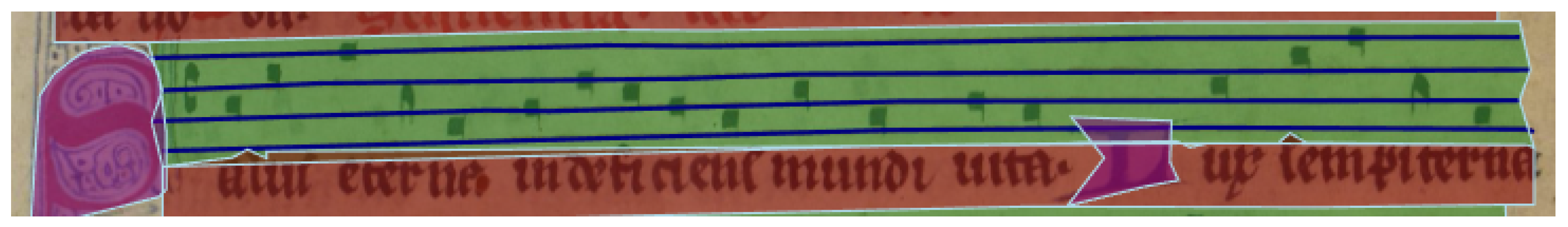
Figure 1.
Staff image written in square notation of the Pa904 (Page 13) dataset. One instance for each class has been marked with a small white number in the picture. There are no instances for the classes F-clef, sharp- and natural-accidental in the example image.
Figure 1.
Staff image written in square notation of the Pa904 (Page 13) dataset. One instance for each class has been marked with a small white number in the picture. There are no instances for the classes F-clef, sharp- and natural-accidental in the example image.

Figure 2.
Sample example pages for the used datasets.

Figure 3.
The schematic workflow of the proposed symbol detection. Additionally to the input and output of the algorithm, the output of the major intermediate steps is displayed. This includes the staff line extraction from the original images, the padding of the line images and the grayscale conversion. Furthermore, the segmentation and further post-processing steps are shown, which includes the probability map generation, the connected component and finally the symbol extraction. The symbols are segmented two times from the background, using two different thresholds. Squares with an additional red box are “uncertain” symbols, which are used within post-processing to correct errors automatically.

Figure 4.
Common errors of the symbol detection, which are corrected by the post-processing pipeline. The yellow and green boxes indicate whether the symbol is on the staff line or between a staff line. Notes, which also have a red border, are the symbols that are “uncertain” and are used for correcting missing symbols in the baseline symbols. The green, red and purple overlay indicates the region. Areas in the first image with green overlay are music-, red are lyric- and purple are drop capital regions. The numbers (1, 2, 4a, 4b, 5a, 5b, 5c, 6) under each image refer to the post-processing step in Section 5 that is intended to fix this error.

Figure 5.
Example of the layout detection. Red regions are lyric regions. Green areas are music regions and purple areas are drop capital regions. We divided the drop capitals into two classes. Big ornated (left one) and smaller ones, which still clearly intrude the music regions (right one).
Figure 5.
Example of the layout detection. Red regions are lyric regions. Green areas are music regions and purple areas are drop capital regions. We divided the drop capitals into two classes. Big ornated (left one) and smaller ones, which still clearly intrude the music regions (right one).


Table 1.
Overview of dataset properties (Nevers P1 means Part 1). All datasets except Pa904 consist of 8 classes (Notes: looped, gapped, neume start; Clef: C-Clef, F-Clef, Accents: Flat, Sharp and Natural). For Pa904, graphical connections between notes (GCN) are not annotated, resulting in only 6 classes.
| Dataset | Pages | Symbols | Symbols/Page | Clefs | Accidentals | GCN Annotated? |
|---|---|---|---|---|---|---|
| Nevers P1 | 14 | 3911 | 279 | 152 | 24 | Yes |
| Nevers P2 | 27 | 10,265 | 380 | 345 | 37 | Yes |
| Nevers P3 | 8 | 1669 | 209 | 83 | 1 | Yes |
| Latin14819 | 182 | 34,762 | 191 | 2108 | 291 | Yes |
| Pa904 | 20 | 9025 | 451 | 264 | 28 | No |
Table 2.
Overview of the evaluated architectures. For each architecture, the publication is cited that describes it. Some architectures have been expanded to include a decoder part so that they reflect a U-Net. In addition, the number of parameters is specified and states whether there were pre-trained weights for the encoder part available.
| Id | Encoder | Decoder | Parameters | ImageNet-Weights |
|---|---|---|---|---|
| FCN | [12] | [12] | 603,649 | None |
| U-Net | [1] | [1] | 31,032,265 | None |
| MobileNet | [18] | Own | 6,584,033 | Encoder |
| ResNet | [19] | Own | 34,345,545 | Encoder |
| Eff-b1 (https://github.com/qubvel/efficientnet, accessed on 30 May 2022) | [20] | Own | 6,237,253 | Encoder |
| Eff-b3 (https://github.com/qubvel/efficientnet, accessed on 30 May 2022) | [20] | Own | 7,851,275 | Encoder |
| Eff-b5 (https://github.com/qubvel/efficientnet, accessed on 30 May 2022) | [20] | Own | 12,005,305 | Encoder |
| Eff-b7 (https://github.com/qubvel/efficientnet, accessed on 30 May 2022) | [20] | Own | 20,141,881 | Encoder |
Table 3.
Overview of the qualitative evaluation of the drop capital detection.
| Big Drop Capital | Small Drop Capital | |
|---|---|---|
| TP | 18 | 15 |
| FP | 0 | 0 |
| FN | 1 | 9 |
Table 4.
Preliminary experiments for the symbol detection using different network architectures. All results are the averages of a five fold of each dataset part. The used backbone is stated on the left. The results of the detection accuracy of all symbols, of solely the notes and the clef, the type accuracy (Notes: looped, gapped, neume start; Clef: C-Clef, F-Clef), the position in staff accuracy of notes and clefs and the , and , given in percent are computed using all datasets except the Pa904. The bold numbers highlight the best value for each metric.
| Detection | Type | Position in Staff | Sequence | |||||||||
|---|---|---|---|---|---|---|---|---|---|---|---|---|
| Archit. | ||||||||||||
| Non Post-proc. | FCN | 97.9 | 98.1 | 93.0 | 23.0 | 97.7 | 99.0 | 98.8 | 99.8 | 94.4 | 92.4 | 84.6 |
| MobileNet | 98.4 | 98.5 | 96.4 | 75.0 | 97.8 | 99.1 | 98.9 | 99.7 | 95.4 | 93.5 | 89.6 | |
| ResNet | 98.8 | 98.9 | 97.3 | 80.2 | 98.0 | 99.2 | 98.9 | 99.8 | 96.2 | 94.5 | 91.9 | |
| Eff-b1 | 98.7 | 98.8 | 97.0 | 87.6 | 98.3 | 99.1 | 98.9 | 99.8 | 96.3 | 94.7 | 91.7 | |
| Eff-b3 | 99.0 | 99.0 | 97.5 | 89.8 | 98.1 | 99.5 | 98.9 | 99.8 | 96.7 | 95.1 | 92.8 | |
| Eff-b5 | 99.0 | 99.0 | 97.8 | 89.7 | 98.2 | 99.5 | 98.9 | 99.7 | 96.7 | 95.1 | 93.6 | |
| Eff-b7 | 99.1 | 99.1 | 98.0 | 90.0 | 98.3 | 99.4 | 99.0 | 99.8 | 96.7 | 95.3 | 93.8 | |
| U-Net | 99.2 | 99.3 | 98.2 | 86.0 | 98.4 | 99.1 | 99.0 | 99.8 | 97.2 | 95.8 | 94.1 | |
| Mean | 98.6 | 98.8 | 96.9 | 77.7 | 98.1 | 99.2 | 98.9 | 99.8 | 96.2 | 94.5 | 91.5 | |
| Post-proc. | FCN | 98.1 | 98.5 | 95.0 | 23.0 | 97.5 | 98.1 | 98.8 | 99.6 | 95.1 | 93.0 | 89.2 |
| MobileNet | 98.5 | 98.6 | 97.0 | 74.4 | 97.4 | 99.0 | 99.1 | 99.8 | 95.8 | 93.8 | 92.5 | |
| ResNet | 98.9 | 99.0 | 97.8 | 80.2 | 97.7 | 99.1 | 99.1 | 99.8 | 96.7 | 94.8 | 94.2 | |
| Eff-b1 | 98.8 | 98.9 | 97.4 | 86.8 | 98.0 | 99.2 | 99.1 | 99.8 | 96.5 | 94.9 | 94.0 | |
| Eff-b3 | 99.1 | 99.1 | 97.7 | 88.6 | 97.8 | 99.3 | 99.1 | 99.8 | 96.7 | 95.0 | 94.4 | |
| Eff-b5 | 99.0 | 99.1 | 98.0 | 89.9 | 97.9 | 99.6 | 99.1 | 99.9 | 97.0 | 95.2 | 95.3 | |
| Eff-b7 | 99.1 | 99.2 | 98.1 | 90.0 | 98.0 | 99.1 | 99.0 | 99.9 | 96.8 | 95.2 | 94.7 | |
| U-Net | 99.3 | 99.4 | 98.2 | 87.0 | 98.0 | 99.3 | 99.2 | 99.9 | 97.3 | 95.7 | 95.1 | |
| Mean | 98.9 | 99.0 | 97.4 | 77.5 | 97.9 | 99.1 | 95.0 | 99.8 | 96.5 | 94.7 | 93.7 | |
Table 5.
Experiments on the Nevers dataset, which was used for evaluation in [12]. Using the post-processing pipeline, the dSAR has improved by about 1%. The melody accuracy rate has improved by 8%. Using more advanced encoders, the mAR could further be improved by about 3%.
Table 5.
Experiments on the Nevers dataset, which was used for evaluation in [12]. Using the post-processing pipeline, the dSAR has improved by about 1%. The melody accuracy rate has improved by 8%. Using more advanced encoders, the mAR could further be improved by about 3%.
| Detection | Type | Position in Staff | Sequence | |||||||||
|---|---|---|---|---|---|---|---|---|---|---|---|---|
| Post-Processing | Archit. | |||||||||||
| no | FCN | 97.8 | 97.9 | 89.5 | 30 | 96.1 | 98.7 | 97.9 | 99.3 | 92.9 | 89.6 | 79.7 |
| Eff-b3 | 98.3 | 98.4 | 94.8 | 65 | 96.3 | 99.2 | 97.8 | 99.4 | 94.1 | 90.9 | 87.7 | |
| yes | FCN | 98.2 | 98.3 | 94.3 | 30 | 95.4 | 98.0 | 98.0 | 99.2 | 93.7 | 90.2 | 88.0 |
| Eff-b3 | 98.6 | 98.6 | 96.4 | 65 | 95.6 | 99.3 | 97.9 | 99.8 | 94.5 | 91.1 | 91.3 | |
Table 6.
In this experiment, training and evaluating was conducted only on the Pa904 dataset (all metrics in %). The mixed model of the previous experiment was optionally used for a document specific fine-tuning. This experiment is most similar to a real world scenario, where only a limited number of pages for training is available.
| Detection | Type | Position in Staff | Sequence | |||||||||
|---|---|---|---|---|---|---|---|---|---|---|---|---|
| Archit. | ||||||||||||
| No Post-proc. | FCN | 99.1 | 99.2 | 93.2 | 22.2 | n/a | 96.9 | 95.8 | 1 | 93.3 | n/a | 84.8 |
| Eff-b3 | 99.6 | 99.6 | 98.0 | 39.9 | n/a | 97.5 | 95.7 | 1 | 94.0 | n/a | 91.2 | |
| Eff-b7 | 99.4 | 99.5 | 97.4 | 23.8 | n/a | 97.6 | 95.7 | 1 | 93.8 | n/a | 91.4 | |
| U-Net | 99.3 | 99.3 | 96.0 | 36.2 | n/a | 96.5 | 95.5 | 1 | 93.3 | n/a | 87.8 | |
| Mean | 99.3 | 99.4 | 96.2 | 29.5 | n/a | 97.1 | 95.7 | 1 | 93.6 | n/a | 88.3 | |
| Post-proc. | FCN | 99.2 | 99.3 | 97.0 | 22.2 | n/a | 95.3 | 98.8 | 1 | 96.4 | n/a | 91.3 |
| Eff-b3 | 99.6 | 99.7 | 98.0 | 39.9 | n/a | 97.0 | 98.8 | 1 | 97.0 | n/a | 94.0 | |
| Eff-b7 | 99.5 | 99.6 | 98.7 | 23.8 | n/a | 97.7 | 98.5 | 1 | 96.7 | n/a | 92.4 | |
| U-Net | 99.5 | 99.6 | 98.0 | 36.2 | n/a | 95.4 | 98.6 | 1 | 96.6 | n/a | 94.7 | |
| Mean | 99.4 | 99.6 | 97.9 | 29.9 | n/a | 96.4 | 98.7 | 1 | 96.7 | n/a | 93.1 | |
| Fine-tuning + No Post-proc. | FCN | 99.1 | 99.2 | 96.0 | 0.03 | n/a | 98.7 | 98.8 | 1 | 93.8 | n/a | 88.8 |
| Eff-b3 | 99.5 | 99.6 | 98.0 | 33.3 | n/a | 98.0 | 98.8 | 1 | 94.5 | n/a | 90.5 | |
| Eff-b7 | 99.5 | 99.6 | 98.7 | 34.7 | n/a | 95.3 | 98.5 | 1 | 94.4 | n/a | 90.3 | |
| U-Net | 99.5 | 99.5 | 97.0 | 32.3 | n/a | 97.0 | 98.6 | 1 | 94.4 | n/a | 90.3 | |
| Mean | 99.4 | 99.5 | 97.4 | 25.1 | n/a | 97.3 | 98.7 | 1 | 94.3 | n/a | 90.0 | |
| Fine-tuning + Post-proc. | FCN | 99.2 | 99.2 | 98.3 | 26.7 | n/a | 97.9 | 98.7 | 1 | 96.6 | n/a | 94.6 |
| Eff-b3 | 99.5 | 99.6 | 98.8 | 33.3 | n/a | 98.0 | 99.0 | 1 | 97.4 | n/a | 95.8 | |
| Eff-b7 | 99.5 | 99.6 | 98.0 | 34.7 | n/a | 95.3 | 98.9 | 1 | 97.3 | n/a | 93.0 | |
| U-Net | 99.5 | 99.6 | 98.5 | 32.3 | n/a | 97.0 | 99.0 | 1 | 97.3 | n/a | 94.3 | |
| Mean | 99.4 | 99.5 | 98.4 | 31.8 | n/a | 97.1 | 98.9 | 1 | 97.2 | n/a | 94.4 | |
Table 7.
Mixed model experiments on the Pa904 dataset with and without post-processing; that is, no training data for fine-tuning were used. Only the model of Table 4 was used for predictions and evaluated solely on the Pa904 dataset (all metrics in %). The recognition rate of the accidents is very low, especially with the FCN, since this was already low in the “mixed model” due to the low amount of training instances.
| Detection | Type | Position in Staff | Sequence | |||||||||
|---|---|---|---|---|---|---|---|---|---|---|---|---|
| Post-Processing | Archit. | |||||||||||
| no | FCN | 98.3 | 98.4 | 93.3 | 3.0 | n/a | 96.4 | 96.7 | 1 | 93.0 | n/a | 84.4 |
| Eff-b3 | 99.2 | 99.4 | 98.3 | 48.0 | n/a | 96.4 | 96.9 | 99.9 | 95.0 | n/a | 90.4 | |
| yes | FCN | 98.5 | 98.6 | 96.2 | 3.0 | n/a | 94.9 | 98.9 | 1 | 95.3 | n/a | 89.4 |
| Eff-b3 | 99.3 | 99.4 | 99.1 | 46 | n/a | 96.1 | 98.9 | 1 | 97.0 | n/a | 93.2 | |
Table 8.
Influence of the individual post-processing steps on the mAR in % of the Pa904 dataset. Each post-processing step is evaluated individually. The entry marked with a plus has improved, but the improvement was too small to be shown in the table. Two models are evaluated: The “Document specific” model which adds a document specific fine-tuning to the mixed model and the “Mixed model“, without fine-tuning, which has been trained on different datasets and subsequently evaluated on this dataset.
| Model | Document Specific (Section 8.3) | Mixed Model (Section 8.4) | ||
|---|---|---|---|---|
| Architecture | FCN | Eff-b3 | FCN | Eff-b3 |
| Post-processing step (compare Section 5) | ||||
| None | 88.8 | 90.5 | 84.4 | 90.4 |
| (1) Correct symbols in wrong layout blocks | 88.8+ | 90.5 | 84.5 | 90.4 |
| (2) Correct overlapping symbols | 89.3 | 90.6 | 84.7 | 90.5 |
| (3) Correct position in staff of clefs | 88.8 | 90.5 | 84.6 | 90.4 |
| (4) Correct missing clefs | 91.2 | 91.8 | 86.3 | 91.3 |
| (5) Correct looped graphical connection | n/a | n/a | 85.9 | 90.7 |
| (6) Correct PIS of stacked notes | 91.3 | 93.2 | 87.8 | 92.5 |
| All combined | 94.6 | 95.8 | 89.4 | 93.2 |
Table 9.
Listing of symbol segmentation error types of the models and their quantity in %. The +/− columns indicate the improvement percentage by which the error type can be reduced by post-processing. The best performing model of the “FCN” and the “Eff-b3” architecture were used (fine-tuning + post-processing). The edit-distance of the predicted sequence and the GT without the usage of replacements is computed. Thus, PIS errors were treated as a TP and a FP.
| FCN | +/− | Eff-b3 | +/− | ||||
|---|---|---|---|---|---|---|---|
| Post-proc. | no | yes | no | yes | |||
| TP (hsar) | 93.78 | 96.59 | 94.55 | 97.42 | |||
| FN | Missing Notes | 1.10 | 1.10 | 0% | 0.93 | 0.74 | 20% |
| Wrong PiS | 2.08 | 0.74 | 64% | 1.80 | 0.63 | 65% | |
| Missing Clef | 0.14 | 0.10 | 28% | 0.08 | 0.05 | 29% | |
| Missing Accid | 0.16 | 0.16 | 0% | 0.09 | 0.09 | 0% | |
| Sum | 3.48 | 2.10 | 39% | 2.90 | 1.51 | 48% | |
| FP | Add. Notes | 0.63 | 0.52 | 17% | 0.71 | 0.39 | 45% |
| Wrong PiS | 2.08 | 0.74 | 64% | 1.80 | 0.63 | 65% | |
| Add. Clef | 0.04 | 0.03 | 9% | 0.04 | 0.04 | 0% | |
| Add. Accid | 0 | 0 | 0% | 0 | 0 | 0% | |
| Sum | 2.75 | 1.30 | 53% | 2.55 | 1.06 | 59% | |
| FP + FN | Overall Sum | 6.23 | 3.40 | 45% | 5.45 | 2.57 | 53% |
Table 10.
Break down of FP and FN errors for additional and missing notes into several causes, which amount for 15.1% and 28.8% of the errors, respectively.
Table 10.
Break down of FP and FN errors for additional and missing notes into several causes, which amount for 15.1% and 28.8% of the errors, respectively.
| Error Type | FN | Examples | FP | Examples |
|---|---|---|---|---|
| Symbols that are close to the text/Text that is mistaken as symbols | 23% |  | 57% |  |
| Horizontal dense symbols | 23% |  | 0% | |
| Vertically dense symbols | 6% |  | 0% | |
| Faded symbols or noise | 12% |  | 0% | |
| Rare symbols | 16% |  | 0% | |
| Clef mistaken as symbols/symbols mistaken as clef | 5% |  | 29% |  |
| No apparent reason | 4% |  | 0% | |
| Outside of staff lines | 4% |  | 0% | |
| Drop capitals | 3% |  | 14.2% |  |
Publisher’s Note: MDPI stays neutral with regard to jurisdictional claims in published maps and institutional affiliations. |
© 2022 by the authors. Licensee MDPI, Basel, Switzerland. This article is an open access article distributed under the terms and conditions of the Creative Commons Attribution (CC BY) license (https://creativecommons.org/licenses/by/4.0/).
Share and Cite
MDPI and ACS Style
Hartelt, A.; Puppe, F. Optical Medieval Music Recognition Using Background Knowledge. Algorithms 2022, 15, 221. https://0-doi-org.brum.beds.ac.uk/10.3390/a15070221
AMA Style
Hartelt A, Puppe F. Optical Medieval Music Recognition Using Background Knowledge. Algorithms. 2022; 15(7):221. https://0-doi-org.brum.beds.ac.uk/10.3390/a15070221
Chicago/Turabian StyleHartelt, Alexander, and Frank Puppe. 2022. "Optical Medieval Music Recognition Using Background Knowledge" Algorithms 15, no. 7: 221. https://0-doi-org.brum.beds.ac.uk/10.3390/a15070221
Note that from the first issue of 2016, this journal uses article numbers instead of page numbers. See further details here.