
A Greedy Algorithm for Neighborhood Overlap-Based Community Detection

Computer Science, Jackson State University, Jackson, MS 39217, USA
Algorithms 2016, 9(1), 8; https://0-doi-org.brum.beds.ac.uk/10.3390/a9010008
Submission received: 24 October 2015
/
Revised: 1 January 2016
/
Accepted: 6 January 2016
/
Published: 11 January 2016
(This article belongs to the Special Issue Algorithms for Complex Network Analysis)
Abstract
:The neighborhood overlap (NOVER) of an edge u-v is defined as the ratio of the number of nodes who are neighbors for both u and v to that of the number of nodes who are neighbors of at least u or v. In this paper, we hypothesize that an edge u-v with a lower NOVER score bridges two or more sets of vertices, with very few edges (other than u-v) connecting vertices from one set to another set. Accordingly, we propose a greedy algorithm of iteratively removing the edges of a network in the increasing order of their neighborhood overlap and calculating the modularity score of the resulting network component(s) after the removal of each edge. The network component(s) that have the largest cumulative modularity score are identified as the different communities of the network. We evaluate the performance of the proposed NOVER-based community detection algorithm on nine real-world network graphs and compare the performance against the multi-level aggregation-based Louvain algorithm, as well as the original and time-efficient versions of the edge betweenness-based Girvan-Newman (GN) community detection algorithm.
1. Introduction
Community detection is one of the classical problems of complex network analysis. A community in a network graph is a subset of the vertices that have a relatively larger density of edges among themselves than to the rest of the vertices [1]. The quality of the partitioning of a network into communities is evaluated using a metric called the modularity score [2]; the larger the modularity score, the more appropriate is the partitioning of the vertices into communities. The problem of identifying a partition of the network into communities with the largest modularity score is NP-complete [3]. Several algorithms have been proposed in the literature for community detection and a majority of these are based on the notion of betweenness [4], defined for an edge as the fraction of the shortest paths between any two vertices going through the edge, considered over all pairs of vertices. Edges with high betweenness are typically removed to disintegrate a connected network into two or more components—each of which are considered to form a closely-knit community. Edge betweenness-based algorithms for community detection are typically considered to identify communities with a larger modularity score at the cost of a significantly larger computation time [5]. Another potential weakness of community detection algorithms could be the inability to detect smaller communities (called the resolution limit problem [6]); this weakness is more prominent in multi-level aggregation algorithms (like the Louvain algorithm [7]). To get around this bottleneck, the focus of research in the area of community detection has veered around strategies (e.g., [8,9,10]) that identify the critical edges (the edges that if removed will lead to the identification of closely-knit communities with high modularity score) without essentially running the time-consuming shortest path algorithms for each vertex and for each edge removal [4,5] as well as be able to identify smaller communities that indeed exist in the network being analyzed (in such a way that the overall sum of the modularity scores of the communities do not get significantly lowered).
One edge-based criterion that can be quickly computed and at the same time appears to be quite effective for community detection is the “neighborhood overlap”. The neighborhood overlap [11] for an edge (u, v) is defined as the ratio of the number of nodes that are neighbors of both the vertices u and v to that of the number of nodes that are neighbors of at least one of the two vertices u or v. As one can see from the above definition, the neighborhood overlap of an edge can be computed just based on the local neighborhood information of the end vertices of the edge and no global knowledge is required. An edge (u, v) that has a smaller value for the neighborhood overlap is more likely to play a significant role in facilitating communication between u and v as well as between vertices that are in the vicinity (i.e., one or more hops) of u and vertices that are in the vicinity of v. The sub graph of vertices involving u and the sub graph of vertices involving v are more likely to have fewer edges connecting them; otherwise, the edge (u, v) would have had a larger neighborhood overlap. Edges having a lower neighborhood overlap are thus referred to as “weak ties” [11] and are often considered for removal to disintegrate a connected network to two or more components—each of which form a community.
The currently known approach [11] of utilizing weak ties and neighborhood overlap for community detection involves fixing a threshold value for the neighborhood overlap and all edges in which neighborhood overlap is less than this threshold value are categorized as weak ties and the rest of the edges are categorized as strong ties. All of these weak ties are removed from the network and the resulting network components form the different communities for the network, referred to as the “partition” of the network. The main problem with the above approach is the issue of fixing an appropriate threshold value for the neighborhood overlap of an edge to identify the weak ties. A larger value for the threshold neighborhood overlap could unnecessarily disintegrate the network into several components (most of them being of smaller size), and the cumulative modularity score of the communities (each community has a modularity score; we define the cumulative modularity score as the sum of the modularity scores of all the communities in a network) could be significantly lower than the optimal value. Likewise, a smaller value for the threshold neighborhood overlap could lead to the coexistence of two potentially different communities as one community, leading to a reduction in the cumulative modularity score.
Our contributions in this paper are as follows: (i) We propose a greedy algorithm of iteratively removing the edges in the increasing order of their neighborhood overlap and choosing the partition of communities that sustains the largest cumulative modularity score. The neighborhood overlap of the edge whose removal leads to the identification of the partition with the largest cumulative modularity score is referred to as the threshold neighborhood overlap and the edges removed until then are referred to as weak ties. It is sufficient that the neighborhood overlap of the edges be computed at the beginning of the algorithm and need not be computed after each edge removal. This a characteristic aspect of our proposed algorithm, unlike the well-known edge-betweenness based Girvan-Newman algorithm [4] and its various improvised versions (e.g., [8,9]) that require the betweenness of the edges to be recomputed after each edge removal. The complexity of the Girvan-Newman algorithm is O(|E| × |V| × (|E| + |V|)) on a graph of |V| vertices and |E| edges [4]. The cumulative modularity score of the communities obtained with our proposed Neighborhood OVERlap-based edge removal (NOVER) algorithm is observed to be only at most 60% lower than the cumulative modularity score obtained with the Girvan-Newman algorithm, whereas the time-complexity of NOVER is O(|E| × (|E| + |V|)) and the actual execution time of the NOVER algorithm has been observed to be as small as just 1% of the execution time of the original Girvan-Newman algorithm on larger real-world networks. The time-complexity of NOVER is thus bound to be significantly smaller than that of the well-known Girvan-Newman algorithm (as large as by a factor of the number of vertices in the graph). Nevertheless, the relative similarity of the communities (quantified on the basis of the Normalized Mutual Information score [12]) detected by the NOVER algorithm and the Girvan-Newman algorithm is observed to be significantly high; (ii) As part of the performance evaluation studies, we propose a novel metric called the Modularity-Resolution-Execution Time-Nodes (MREN) score—defined quantitatively as the ratio of the product of the cumulative modularity score and the fraction of communities of the smallest size to that of the product of the execution time of the algorithm and the number of nodes in the network. We propose the MREN score to be used as a global metric (irrespective of the number of nodes in the network) for evaluating the effectiveness of an algorithm to detect communities with respect to modularity maximization, resolution limit (detecting smaller communities) and execution time. We claim that larger the MREN score for a community detection algorithm on a real-world network, the more effective is the algorithm with respect to simultaneously satisfying all of the above three performance criteria. We evaluate the MREN scores of the community detection algorithms on nine different real-world networks and observe the NOVER algorithm to incur the largest MREN score for eight of these networks.
To the best of our knowledge, we have not come across such a formal time-efficient and effective algorithm that uses neighborhood overlap as the basis for community detection. The rest of the paper is organized as follows: Section 2 introduces the terms neighborhood overlap, weak ties and modularity score with appropriate examples. Section 3 explains in detail the proposed NOVER algorithm with an example. Section 4 explains the working of the well-known Girvan-Newman (GN) algorithm (both the original and time-efficient versions) for edge betweenness based community detection as well as the working of the Louvain multi-level aggregation algorithm. Section 5 presents the simulation results evaluating the performance of the NOVER algorithm vis-à-vis the Louvain, GN-original and GN-efficient versions on real-world network graphs with respect to the cumulative modularity score of the communities detected, resolution limit, execution time and extent of similarity. Section 6 reviews related work in the literature on community detection using edge betweenness and neighborhood overlap. Section 7 concludes the paper and outlines ideas for future work. Throughout the paper, the terms “vertex” and “node”, “edge” and “link”, “community” and “component” are used interchangeably. They mean the same.
2. Terminology and Examples
In this section, we introduce the three key terms used in this paper and explain their calculation with examples. These are: Neighborhood Overlap, Weak Ties and Modularity Score.
2.1. Neighborhood Overlap and Weak Ties
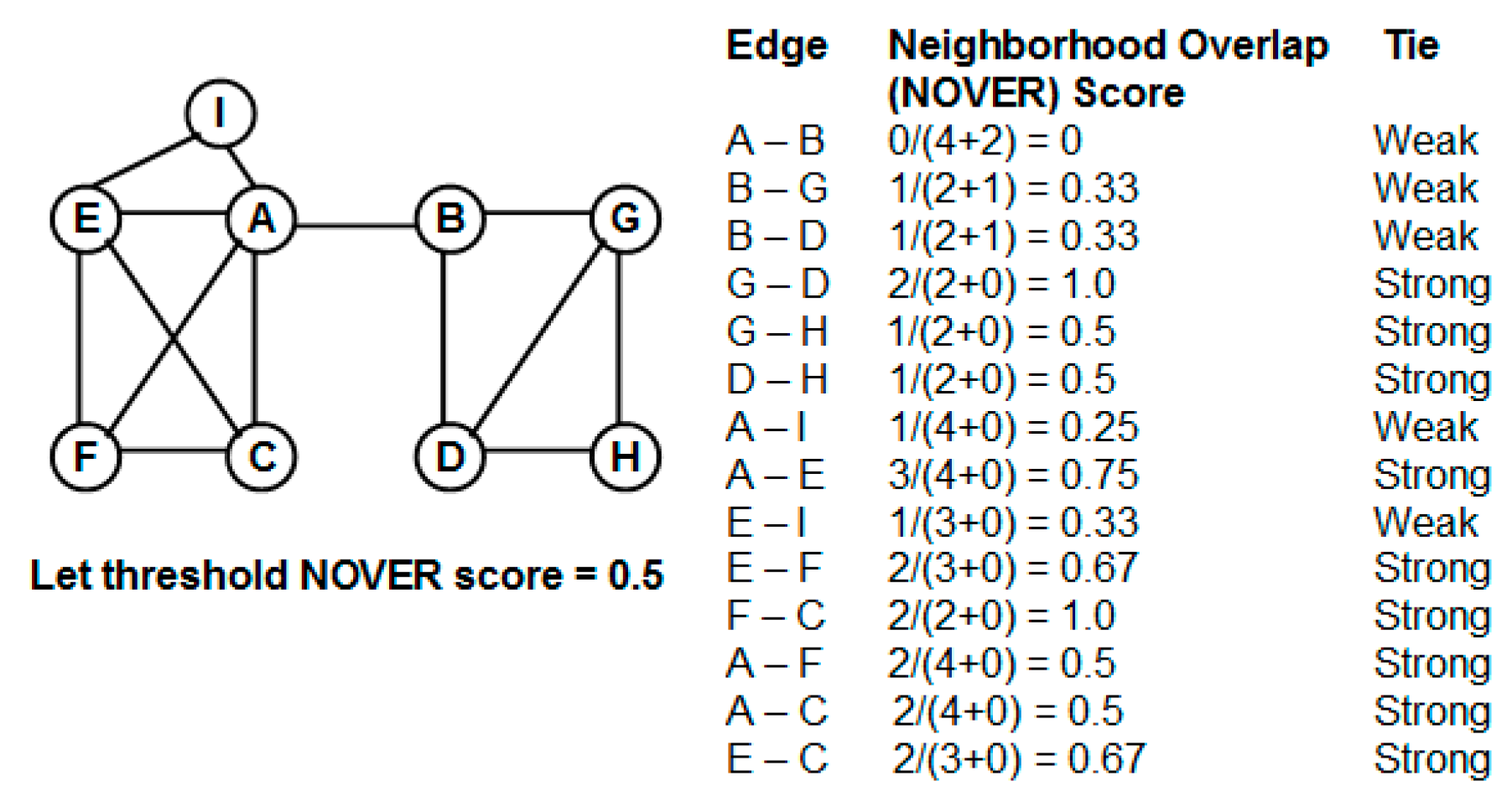
The neighborhood overlap (NOVER) of an edge (u, v) [11,13] is defined as the number of vertices who are common neighbors of both u and v divided by the number of vertices who are neighbors of at least one of the two vertices u or v (excluding each other). Quantitatively,
where ku and kv are, respectively, the degrees of nodes u and v, and cuv is the number of common neighbors of both u and v. The factor of 2 in the denominator is to account for excluding vertices u and v who are neighbors of each other. It is obvious that the NOVER values range from 0 to 1. The convention followed in the literature until now [11] is that edges with NOVER value below a threshold are classified as weak ties and the rest of the edges are classified as strong ties. An appropriate choice for this threshold value is very difficult to be fixed and depends on several characteristics (like the degree distribution of the nodes and the edge-to-node ratio, as seen in our simulation results) of the underlying network considered. Figure 1 illustrates an example to calculate the NOVER scores for the edges in a graph and their classification (as weak or strong ties) based on a threshold NOVER score of 0.50.
Figure 1.
Example to illustrate the calculation of the neighborhood overlap score and identification of weak ties.
Figure 1.
Example to illustrate the calculation of the neighborhood overlap score and identification of weak ties.

2.2. Modularity Score
The modularity score [2] of a community C of n vertices v1, v2, ..., vn is defined as:
wherein Ai,j = 1 if there is an edge between two vertices vi and vj and Ai,j = 0 otherwise. Let ki and kj denote the degree of any two vertices vi and vj, and let m be the total number of edges in the graph. Essentially, the formula considers all pairs of vertices vi and vj among the n vertices constituting the community and assigns a positive score of 1 − kikj/(2 × m) if there is an edge between the two vertices vi and vj and a negative score of 0 − kikj/(2 × m) if there is no edge between the two vertices vi and vj. Note that the product of the degree of any two vertices in a graph is less than or equal to twice the number of edges in the graph [14]. Hence, for a pair of vertices vi and vj, the modularity score is in the range (0 ... 1) if there is an edge between vi and vj, and the modularity score is in the range (−1, ..., 0) if there is no edge between the pair vi and vj. The cumulative modularity score [2] of a partition of the network into p communities is the sum of the modularity scores of the individual communities, defined as:
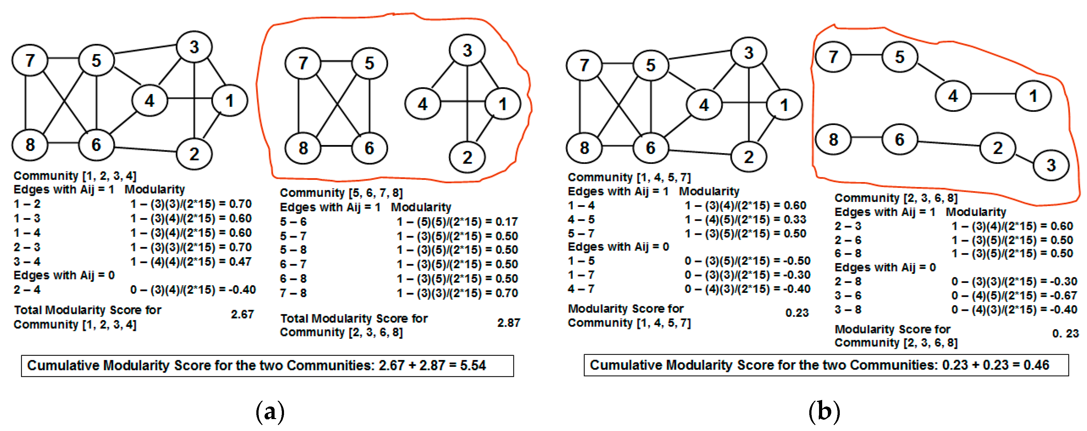
Figure 2.
Example to illustrate the calculation of modularity scores of communities. (a) Partition with high cumulative modularity score; (b) Partition with low cumulative modularity score.
Figure 2.
Example to illustrate the calculation of modularity scores of communities. (a) Partition with high cumulative modularity score; (b) Partition with low cumulative modularity score.

Figure 2 illustrates the calculation of the cumulative modularity scores for two different partitions of a graph. The first partition (i) is a more appropriate split of the vertices into two communities (there are more edges among vertices within a community compared to the number of edges crossing the two communities) and hence has a higher modularity score (both the individual community modularity scores and the cumulative modularity score are high) compared to the second partition (ii) for which there are more edges crossing the two communities compared to the number of edges between vertices within the individual communities.
3. Neighborhood OVERlap (NOVER)-Based Community Detection Algorithm
In this section, we first motivate the weakness associated with the currently adopted approach of fixing a threshold neighborhood overlap (NOVER) score for community detection with an example. We then describe the proposed NOVER-based community detection algorithm in detail along with its run-time analysis and an illustrative example.
3.1. Motivation
The motivation for our proposed algorithm is that the trial-and-error approach of fixing a threshold NOVER value (to classify edges as weak ties and strong ties) and removing the weak ties to obtain a partition of the vertices into communities may not always yield a highly modular partition of the vertices (such that the cumulative modularity score is as large as possible) in the first trial itself. We may have to attempt at fixing different threshold values and evaluate the cumulative modularity scores for each of the different partitions before selecting the partition with the largest cumulative modularity score. At the worst case, there is an infinitely large possible values for the threshold NOVER score in the range (0 ... 1) and one cannot try each of these values before arriving at a partition with the largest cumulative modularity score.
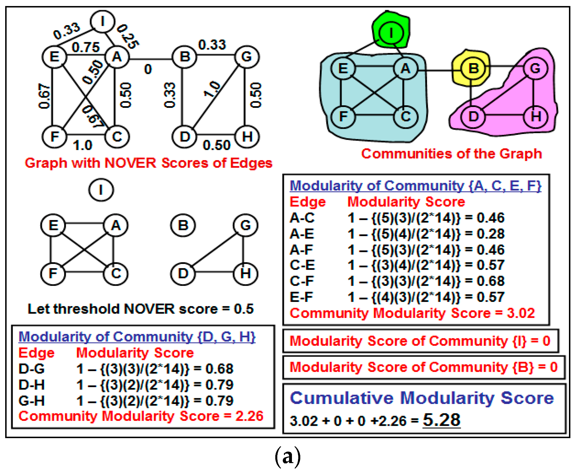
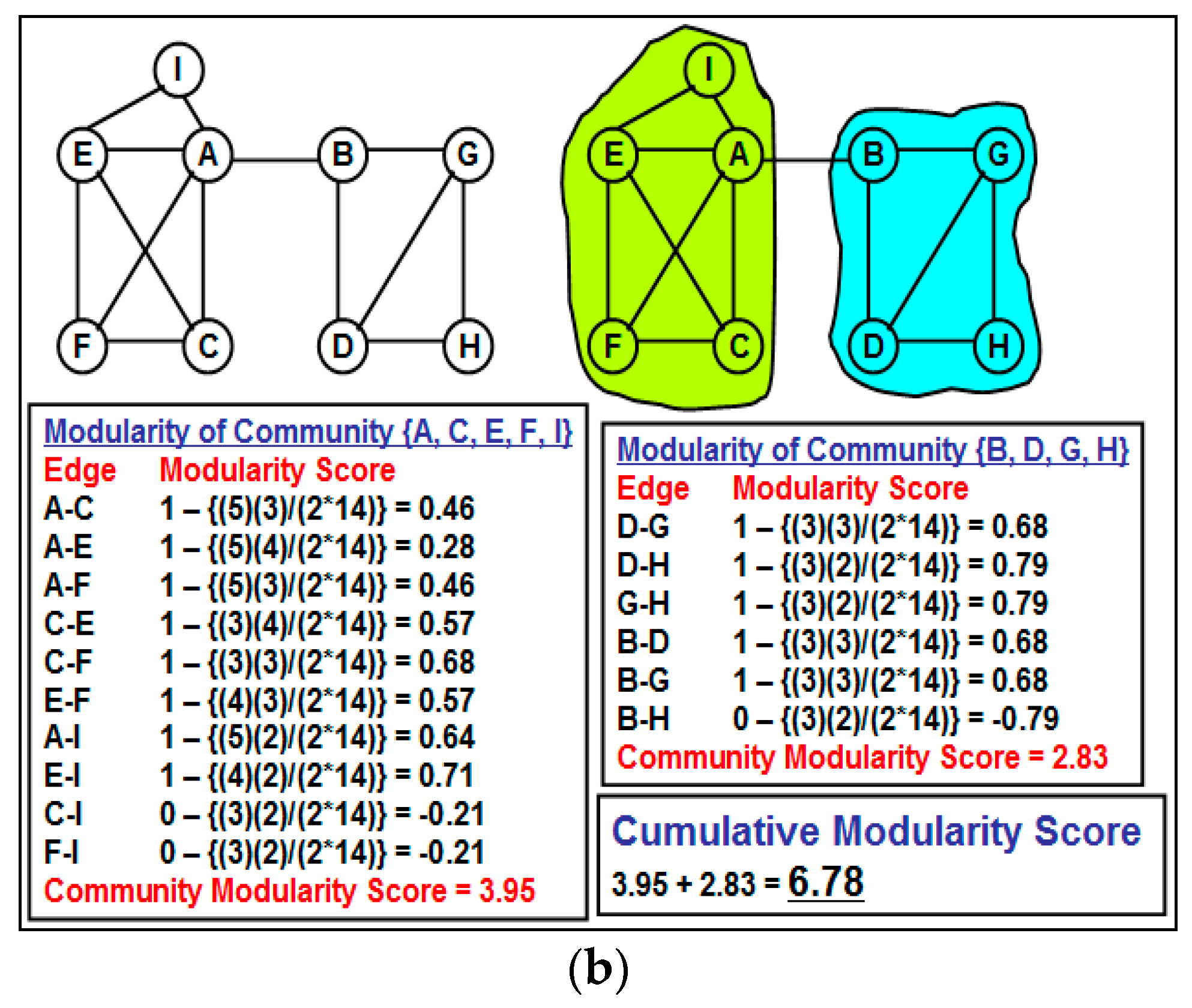
Figure 3 illustrates a motivating scenario of partitioning the graph (the value adjacent to each edge is the NOVER score for the edge) based on an inappropriate threshold NOVER value of 0.5: the cumulative modularity score of the set of communities {{I}, {B}, {A, E, F, C}, {D, G, H}} obtained by removing all edges with NOVER scores less than or equal to 0.5 is lower than the cumulative modularity score of the set of communities {{A, E, F, C, I}, {B, D, G, H}}. The example thus motivates the need for a formal algorithm to detect communities based on the NOVER scores of the edges rather than removing all edges whose NOVER scores are less than or equal to a threshold value and claiming the resulting partitions as different communities.
Figure 3.
Motivating example to illustrate the impact of not choosing an appropriate threshold value for the neighborhood overlap score to partition the Network into communities. (a) A greedy approach of removing all edges with NOVER score less than or equal to the threshold; (b) A better partition of the vertices into communities with a relatively larger cumulative modularity score.


3.2. NOVER Algorithm
Our objective in this paper is to develop a formal and organized algorithm for using the NOVER scores to determine a highly modular partitioning of the vertices into communities instead of adopting a trial-and-error approach to determine a partitioning of the vertices into communities based on each possible threshold NOVER value for the edges. In this pursuit, we propose that instead of fixing a threshold NOVER value and removing the edges with NOVER value less than the threshold to obtain a partition, we would rather iteratively remove one edge at a time (in the increasing order of their NOVER values) and evaluate the cumulative modularity score of the resulting partition. As we remove the edges, one at a time, we keep track of the partition that has resulted in the largest cumulative modularity score; at the end, the algorithm returns the partition with the largest cumulative modularity score (referred to as the Threshold Community Partition). Though the proposed algorithm is greedy and is not guaranteed to give the optimal partition for all graphs, we observe the algorithm to determine partitions with cumulative modularity scores that are only at most 60% less than that determined using the well-known Girvan-Newman edge betweenness-based algorithm for community detection, and incurs a time-complexity that is significantly less than that of the Girvan-Newman algorithm (the actual execution time of the NOVER algorithm could be as low as 1% of the execution time of the original Girvan-Newman algorithm). Moreover, on the basis of the NMI scores [12], we observe the communities detected with the NOVER algorithm to be significantly similar (with respect to the composition) to those detected with the Girvan-Newman algorithm.
The proposed algorithm is described as follows (see Algorithm 1 for the high-level pseudo code of the entire algorithm and Algorithms 2–5 for the pseudo codes of the various sub routines). We compute the NOVER scores (Algorithm 2 presents the pseudo code for computing the NOVER scores) of the edges only once, before the first iteration, and store them in a sorted order in a heap-based priority queue, NOVER-List (the edge with the smallest NOVER score is the root of the heap). In each iteration, we remove the edge with the lowest NOVER score (among the edges existing for that iteration) and run the Breadth First Search (BFS) algorithm (see Algorithm 3 for the pseudo code of BFS to determine a connected component) to obtain the various connected components of the graph (see Algorithm 4 for the pseudo code to determine all the connected components of a graph). Note that due to the removal of an edge, the number of components (each component is a community) of a graph could be different than what existed prior to the removal of the edge. A component of a graph is the largest connected sub graph such that inclusion of an additional vertex makes the sub graph disconnected [15]. We compute the modularity scores for each of the resulting communities (see Algorithm 5 for the pseudo code to determine the modularity score for a community) and also compute the cumulative modularity score of the partition (set of communities). We continue with each of the iterations, as described above, and keep track of the partition with the largest cumulative modularity score obtained across the iterations and also keep track of the NOVER score of the edge whose removal lead to the identification of the partition with the largest cumulative modularity score. At the end of all the iterations, all the edges in the graph get removed and the algorithm outputs the partition (referred to as the threshold community partition) with the largest cumulative modularity score and the corresponding NOVER score of the edge (as identified across the iterations).
| Algorithm 1 Neighborhood Overlap-Based Community Detection Algorithm |
Input: Graph G(V, E); Neighbor List N(v) for every vertex v V Output: Threshold Community Partition; Threshold NOVER Score; LargestCumulativeModularity Score Auxiliary Variables: NOVER-List, Threshold Community Partition, Cumulative Modularity Score, Community Modularity Score, Components Initialization: NOVER-List = , Threshold Community Partition = , Largest Cumulative Modularity Score = 0, Cumulative Modularity Score = 0, Community Modularity Score Begin NOVER Algorithm for every edge (u, v) E do NOVER(u, v) = Compute-NOVER-Score(u, v, N(u), N(v)) NOVER-List = NOVER-List {NOVER (u, v); (u, v)} end for while (NOVER-List ≠ ) do Edge (u, v) = ExtractRoot (NOVER-List)//Remove edge (u, v) with the lowest NOVER score E = E − {(u, v)} Cumulative Modularity Score = 0 Components = FindComponents (G, N) for every Component C Components do Community Modularity Score = Compute-Modularity-Score (C, G, N) Cumulative Modularity Score = Cumulative Modularity Score + Community Modularity Score end for if (Largest Cumulative Modularity Score < Cumulative Modularity Score) then Largest Cumulative Modularity Score = Cumulative Modularity Score Threshold Community Partition = Components Threshold NOVER Score = NOVER (u, v) end if end while return Threshold Community Partition, Largest Cumulative Modularity Score, Threshold NOVER Score End NOVER Algorithm |
| Algorithm 2 Pseudo Code to Determine Neighborhood Overlap Score for an Edge |
Input: Vertices u and v; Neighbor Lists N(u) and N(v) Output: NOVER (u, v) Auxiliary Variables: Common Neighbors, Total Neighbors Initialization:Common Neighbors = ; Total Neighbors = Begin Compute-NOVER-Score for every vertex I N(u) and i ≠ v do Total Neighbors = Total Neighbors {i} end for for every vertex i N(v) and i ≠ u do if i Total Neighbors then Total Neighbors = Total Neighbors {i} end if if i N(u) then Common Neighbors = Common Neighbors {i} end if end for NOVER (u, v) = |Common Neighbors|/|Total Neighbors| return NOVER(u, v) End Compute-NOVER-Score |
| Algorithm 3 Pseudo Code of the Breadth First Search Algorithm to Determine a Connected Component |
Input: Graph G = (V, E); Starting Vertex s; Neighbor List N(v) for every vertex v V Output: VisitedVertices Auxiliary Variables: FIFOQueue Initialization: FIFOQueue = ; VisitedVertices = Begin BFS FIFOQueue = FIFOQueue {s} VisitedVertices = VisitedVertices {s} while (FIFOQueue ≠ ) do Vertex u = Extract(FIFOQueue)//remove the vertex from the front of the queue for every vertex v N(u) do if v VisitedVertices then VisitedVertices = VisitedVertices {v} FIFOQueue = FIFOQueue {v} end if end for end while return VisitedVertices End BFS |
| Algorithm 4 Pseudo Code to Determine All the Connected Components of a Graph |
Input: Graph G = (V, E); Neighbor List N(v) for every vertex v V Output: Components Auxiliary Variables: VerticesTraversed; VerticesNotTraversed Initialization: Components = , VerticesTraversed = , VerticesNotTraversed = V Begin FindComponents while (|VerticesTraversed| < |V|) do Vertex s = Pick a vertex randomly from the set VerticesNotTraversed Component Vertex set S = BFS(G, N, s)//BFS returns the set of vertices visited for every v Sdo VerticesNotTraversed = VerticesNotTraversed − {v} VerticesTraversed = VerticesTraversed {v} end for Components = Components S end while return Components End FindComponents |
| Algorithm 5 Pseudo Code to Determine the Modularity Score for a Community |
Input: Community C (v1, v2, ..., vn) of n vertices; G = (V, E); Neighbor List N(v) for every vertex v V Output: Community-Modularity-Score Initialization: Community-Modularity-Score = 0, Modularity (u, v) for any pair u, v C Begin Compute-Modularity-Score for every vertex vi Cdo for every vertex vj C and i < j do if (vi, vj) E then Modularity (vi, vj) = 1 − (|N(vi)| × |N(vj)|/(2 × |E|)) else Modularity (vi, vj) = 0 − (|N(vi)| × |N(vj)|/(2 × |E|)) end if Community-Modularity-Score = Community-Modularity-Score + Modularity(vi, vj) end for end for return Community-Modularity-Score End Compute-Modularity-Score |
The BFS algorithm takes Θ(|V| + |E|) time to run on a graph of |V| vertices and |E| edges. We run BFS once for each iteration of the proposed NOVER algorithm and there are a total of |E| iterations (one iteration per edge removal), incurring a time-complexity of Θ(|E| × (|V| + |E|)). It takes Θ(|E| × log|E|) time to construct the NOVER-List (a heap) and then Θ(log|E|) to re-heapify it for each edge removal; the time-complexity of managing the heap is thus Θ(|E| × log|E|). Thus, the time-complexity of the NOVER algorithm is Θ(|E| × log|E| + |E| × (|V| + |E|)) = Θ(|E| × (|V| + |E| + log|E|)). But, since Θ(|E|) is more dominating than Θ(log|E|), we could say the overall time-complexity of the proposed NOVER algorithm is Θ(|E| × (|V| + |E|)).
3.3. Example for the NOVER Algorithm
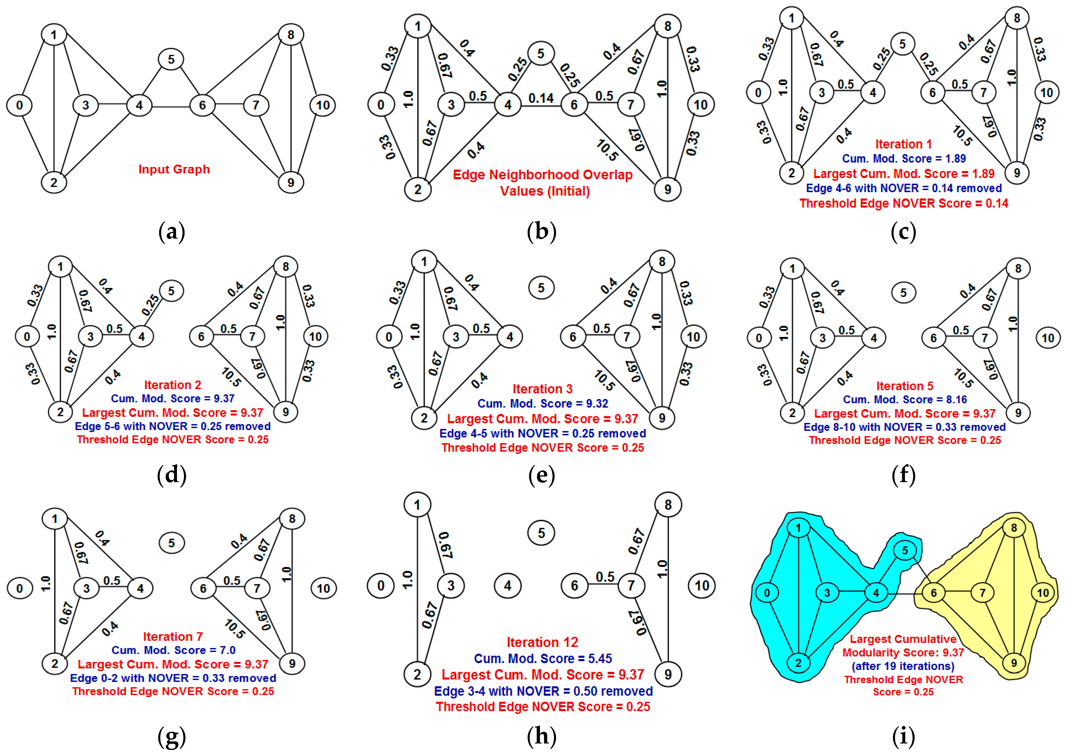
Figure 4 presents an example to illustrate the sequence of iterations of the NOVER algorithm. The Neighborhood Overlap (NOVER) scores for the edges are calculated before the beginning of the first iteration. We remove the edges (one edge removal per iteration) in the increasing order of their NOVER scores. For every edge removal, we identify the various components (each component is a community) of the graph and calculate the modularity score of each community and thence the cumulative modularity score of the partition. If the cumulative modularity score calculated in an iteration exceeds the largest known cumulative modularity score until then (that is the largest known cumulative modularity score prior to the iteration), we update the cumulative modularity score as well as refer to the NOVER score of the edge that contributed to the largest cumulative modularity score as the Threshold NOVER score.
Figure 4.
Example to illustrate the execution of the NOVER algorithm. (a) Input graph; (b) Neighborhood overlap values for the edges in the input graph; (c) At the end of Iteration 1: Remaining edges in the graph after edge 4–6 with NOVER score of 0.14 is removed; (d) At the end of Iteration 2: Remaining edges in the graph after edges 5 and 6 with NOVER score of 0.25 is removed; (e) At the end of Iteration 3: Remaining edges in the graph after edges 4 and 5 with NOVER score of 0.25 is removed; (f) At the end of Iteration 5: Remaining edges in the graph after edge 8-10 with NOVER score of 0.33 is removed; (g) At the end of Iteration 7: Remaining edges in the graph after edge 0–2 with NOVER score of 0.33 is removed; (h) At the end of Iteration 12: Remaining edges in the graph after edges 3 and 4 with NOVER score of 0.50 is removed; (i) At the end of Iteration 19: Final partitioning of the network graph into communities.

We observe the input graph to remain as one single component for the first iteration with a cumulative modularity score of 1.89 and the Threshold NOVER score of 0.14 (corresponds to the NOVER score of the first edge removed). In the second iteration, the removal of edges 5 and 6 with a NOVER score of 0.25 disintegrated the graph into two components {0, 1, 2, 3, 4, 5} and {6, 7, 8, 9, 10} incurring a cumulative modularity score of 9.37 that is greater than the larger cumulative modularity score known until then. We update the largest cumulative modularity score to 9.37 and set the Threshold NOVER score of the edge to 0.25. In the third iteration, we remove edges 4 and 5 that has the same NOVER score as that of the currently known Threshold NOVER score; but, the removal of edges 4 and 5 disintegrates the graph into three communities, with a cumulative modularity score of 9.32, slightly less than the currently known largest cumulative modularity score. Hence, we do not update the largest cumulative modularity score at the end of the third iteration. Further, the edge removals in the subsequent iterations also do not appear to increase the cumulative modularity score of the communities (we only see a reduction in the cumulative modularity score of the communities detected in iterations 3–19). Thus, the best possible partition of the vertices into communities that could incur the largest cumulative modularity score is the partition detected at the end of the second iteration: {0, 1, 2, 3, 4, 5} and {6, 7, 8, 8, 10} with a cumulative modularity score of 9.37 and threshold NOVER edge score of 0.25.
4. Girvan-Newman Algorithm for Edge Betweenness-Based Community Detection
In this section, we briefly review the working of the well-known Girvan-Newman algorithm for edge betweenness-based community detection [4]. The betweenness of an edge is a measure of the fraction of the number of shortest paths going through the edge among all the shortest paths existing between a pair of nodes, considered across any two nodes in the network graph.
4.1. Procedure to Compute the Edge Betweenness
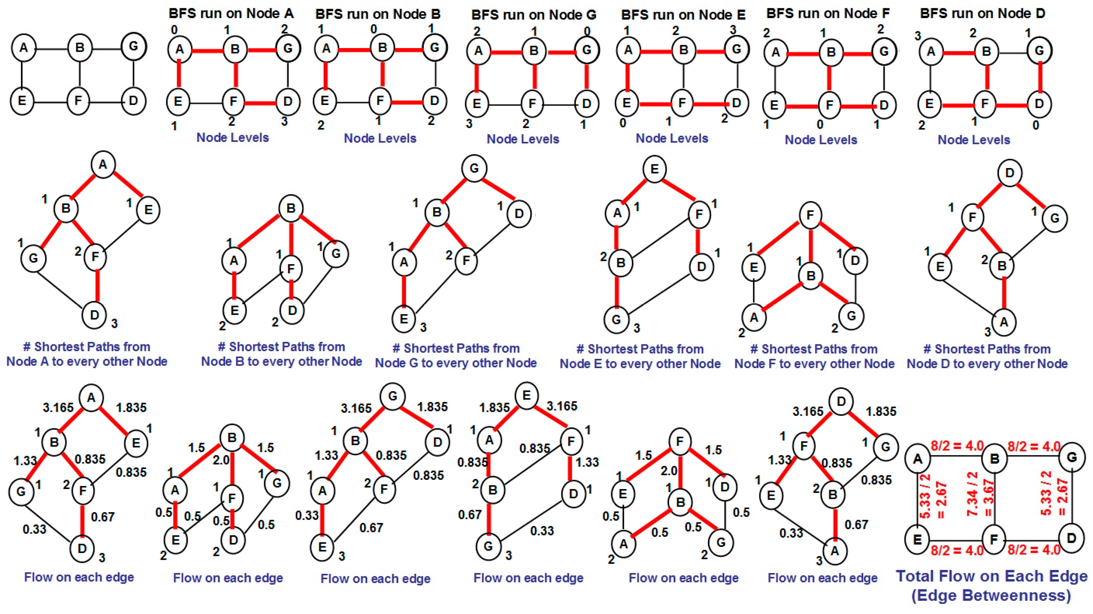
The Girvan-Newman algorithm involves three phases to calculate the betweenness of the edges: (i) We run the Breadth First Search (BFS) algorithm starting from every node in the graph and determine BFS-trees rooted at every node; (ii) For each such BFS-tree rooted at a particular node r, we determine the number of shortest paths from node r to every other node in the network. The number of shortest paths from the root to itself is 1; the number of shortest paths for a node v (at a level l > 0 in the BFS-tree rooted at node r) from the root r (the root is considered to be at level 0) is the sum of the number of shortest paths from the root node r to the predecessor nodes u (at level l − 1 in the BFS-tree rooted at node r) in the original graph; (iii) For each of the BFS-trees, we determine the amount of flow from the root node (say node r) to all the other vertices and thereby determine the amount of flow going through each edge. For each BFS tree, to begin with, we assume one unit of flow originates at each node. We start with the node at the bottommost level and proceed one level at a time, all the way to the root node. For each BFS tree, except the root node, a node at level l aggregates the flow along the edges to nodes at level l + 1, adds its own one unit of flow and proportionally divides the final aggregated flow to its predecessors at level l − 1 in the original graph (based on the number of shortest paths originating from the root node to the predecessor). The total flow through an edge is the sum (for directed graph) or half of the sum (for undirected graph) of the flows determined through that edge when BFS is run from every vertex in the graph. We illustrate the calculation of flow on each edge of a BFS-tree in Figure 5 on an example graph.
We explain the procedure to compute the flow values using a sample BFS tree in Figure 5. Consider the BFS tree rooted at node A. There is only one node (node D) at the bottommost level. Let 1 unit of flow start from node D. Node D gets two of its shortest paths to the root node A through node F and one shortest path through node G. Hence, node D sends 2/3 of the flow to node F and 1/3 of the flow to node G. Node F adds the 2/3 flow received to its own one unit of flow (considered to originate at itself) and splits the resulting 1.67 units of flow equally to its two predecessor nodes B and E (as each of them contribute one shortest path from the root node A) and sends 0.835 to each of nodes B and E. Node G merely adds the 0.33 flow units to the one unit of flow originating at itself and sends 1.33 to nodes B. Node B aggregates the 1.33 and 0.835 units of flow coming along the edges from nodes at the lower level and adds its own one unit of flow and sends 3.165 units of flow to node A. Node E simply adds one unit of flow to the 0.835 units of flow received from node F and sends 1.835 units of flow to node A.
Figure 5.
Example to illustrate the calculation of edge betweenness.

4.2. Original Version of Girvan-Newman Algorithm for Community Detection with Larger Cumulative Modularity Score
The Edge Betweenness-based Girvan-Newman algorithm for community detection is an iterative algorithm that removes one edge per iteration (the edge with the largest betweenness at the beginning of the iteration is removed) and computes the cumulative modularity score of the resulting component(s); as before, each component is considered a community. The partition that incurs the largest cumulative modularity score is kept track of during each iteration. Unlike our proposed NOVER algorithm, the Girvan-Newman algorithm for community detection (referred hereafter as GN-original algorithm) requires the betweenness values of the edges to be recomputed at the end of each iteration. Due to the removal of an edge during a particular iteration, the betweenness of the existing edges in the graph could increase or decrease and this needs to be captured in order to appropriately decide on the edge to be removed in the subsequent iteration.
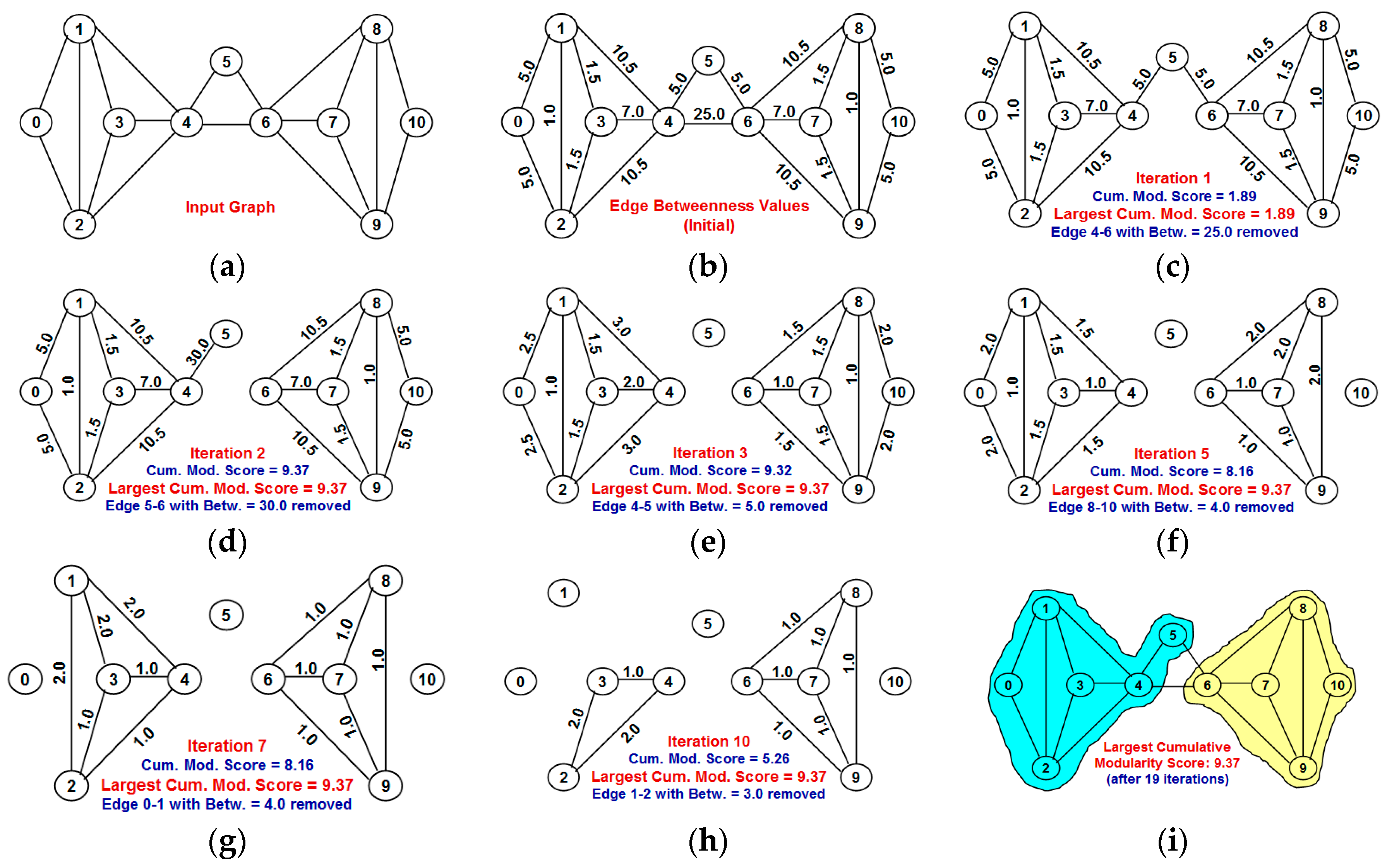
Figure 6 illustrates our application of the GN-original algorithm on the same example graph used in Figure 4 for the NOVER algorithm. For each iteration, the edge weights displayed in the graph corresponds to the edge betweenness values computed after the previous iteration and the edge removed (the edge with the maximum betweenness) for the current iteration is listed below the graph along with its betweenness value. We observe the GN-original and NOVER algorithms to determine an identical partition (as well as the best possible partition) of the vertices into communities.
To compute the betweenness of the edges per iteration, the Θ(|V| + |E|)-BFS algorithm needs to be run on each of the |V| vertices—incurring a time-complexity of Θ(|V| × (|V| + |E|)) per iteration. There are a total of |E| edges in the graph and the above time-complexity is incurred for each edge removal. Hence, the overall time-complexity of the original Girvan-Newman algorithm for community detection is Θ(|E| × |V| × (|V| + |E|)). Note that our proposed NOVER algorithm is of time-complexity Θ(|E| × (|V| + |E|)) and hence is expected to be faster than the GN-original algorithm by a factor of the number of vertices in the graph. For complex real-world networks of larger size (i.e., more nodes), we could expect the NOVER algorithm to run significantly faster than the original Girvan-Newman algorithm for community detection.
Figure 6.
Example to illustrate the original Girvan-Newman algorithm for edge betweenness-based community detection (betweenness of the edges is updated for each iteration). (a) Input graph; (b) Betweenness values for the edges in the input graph; (c) At the end of Iteration 1: Remaining edges in the graph after edge 4–6 with Betweenness score of 25.0 is removed; (d) At the end of Iteration 2: Remaining edges in the graph after edges 5 and 6 with Betweenness score of 30.0 is removed; (e) At the end of Iteration 3: Remaining edges in the graph after edges 4 and 5 with Betweenness score of 5.0 is removed; (f) At the end of Iteration 5: Remaining edges in the graph after edge 8–10 with Betweenness score of 4.0 is removed; (g) At the end of Iteration 7: Remaining edges in the graph after edges 0 and 1 with Betweenness score of 4.0 is removed; (h) At the end of Iteration 10: Remaining edges in the graph after edges 1 and 2 with Betweenness score of 3.0 is removed; (i) At the end of Iteration 19: Final partitioning of the network graph into communities.

4.3. Girvan-Newman Algorithm for Time-Efficient Community Detection
The original Girvan-Newman algorithm for community detection (GN-original algorithm) requires the betweenness of the edges to be recomputed for each iteration of the algorithm (i.e., after each edge removal). This is an expensive overhead. In this paper, we envision a variant of the Girvan-Newman algorithm (referred to as GN-efficient) wherein the edges are removed in the decreasing order of their betweenness values that are computed on the input graph and not updated after each iteration. Such an algorithm would have a time-complexity of only Θ(|V| × (|V| + |E|) + |E| × (|V| + |E|)) = Θ((|V| + |E|)2), as the BFS algorithm needs to be run once for every vertex at the beginning of the algorithm (to determine the initial edge betweenness values) and then once for each iteration (after an edge removal) to extract the components of the graph.
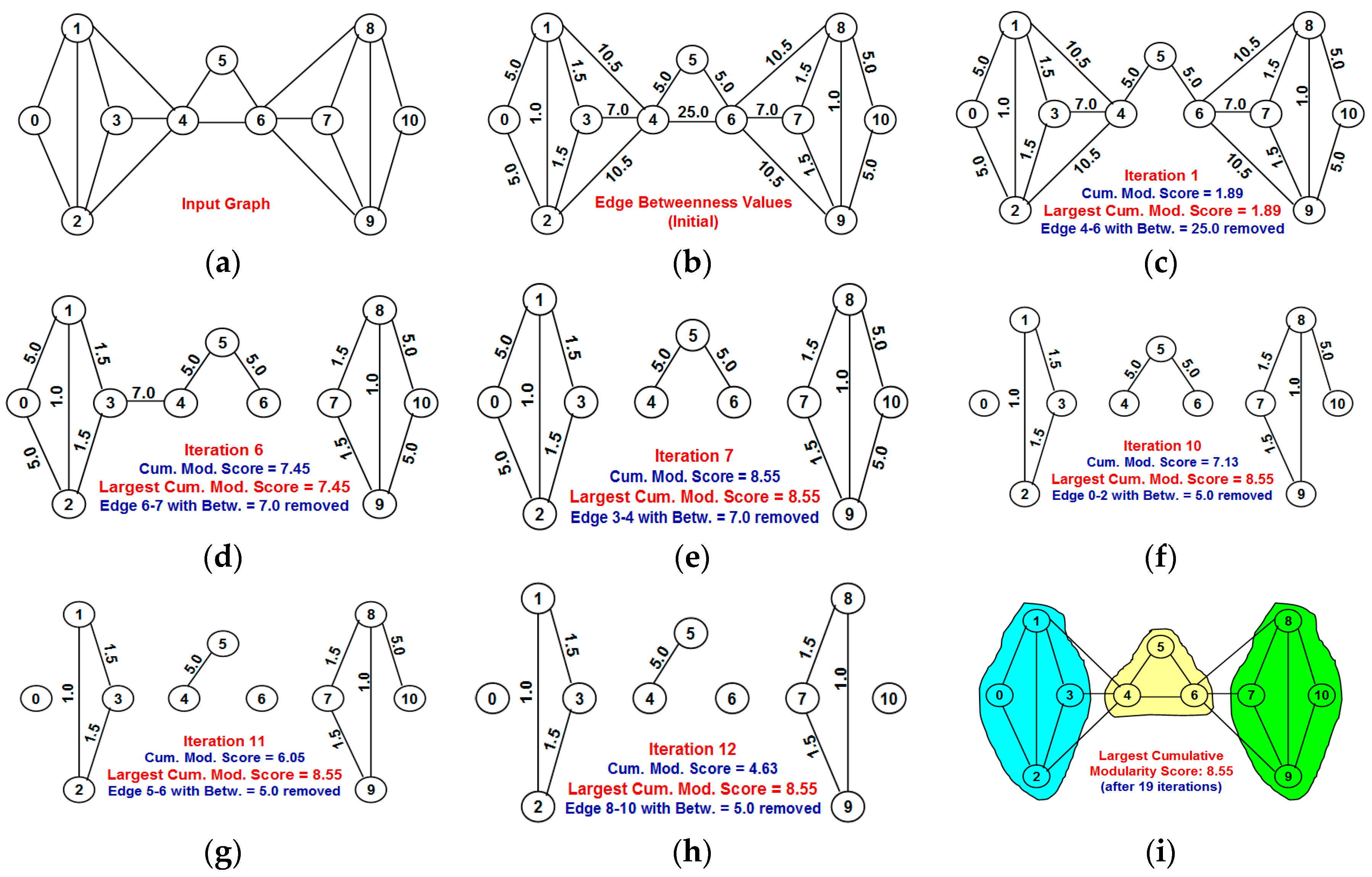
Figure 7 illustrates the execution of the GN-efficient algorithm on the same example graph used in Figure 4 and Figure 6 for the NOVER and GN-original algorithms respectively. One can notice that the initial betweenness values of the two edges 4 and 5, and 5 and 6 are relatively low (value of 5.0 each). However, the removal of edges 4–6 in the first iteration increases the betweenness of the two edges 4 and 5, and 5 and 6 to 30.0 each (refer Figure 6) and no other edge has a betweenness value equal to or larger than 30.0. Hence, in the second iteration, one of these two edges (4 and 5 or 5 and 6) should have been removed (as done in the case of GN-original, Figure 6). However, in the case of the GN-efficient algorithm, since the betweenness of the edges are not updated after each iteration (to save time from running the BFS algorithm starting from each vertex for each iteration), we end up removing edges (1–4, 2–4, 6–8 and 6–9) with betweenness values of 10.5 each, without any improvement in the cumulative modularity score. Iterations 6 and 7 lead to the disintegration of the graph into two and three components (communities) respectively due to the removal of edges 6 and 7, and 3 and 4, each with a betweenness of 7.0. There is no further improvement in the cumulative modularity scores after iteration 7. The final largest possible cumulative modularity score of the communities detected by the GN-efficient algorithm is 8.55 and it is less than the cumulative modularity score of 9.37 of the communities detected by the GN-original and NOVER algorithms. The improvement in the execution time of the GN-efficient algorithm thus appears to come at a possible loss of modularity with respect to detecting communities with the largest cumulative modularity score.
Figure 7.
Example to illustrate Girvan-Newman efficient algorithm for edge betweenness-based community detection (initial edge betweenness values used for each iteration). (a) Input graph; (b) Betweenness values for the edges in the input graph; (c) At the end of Iteration 1: Remaining edges in the graph after edge 4-6 with Betweenness score of 25.0 is removed; (d) At the end of Iteration 6: Remaining edges in the graph after edges 6 and 7 with Betweenness score of 7.0 is removed; (e) At the end of Iteration 7: Remaining edges in the graph after edges 3 and 4 with Betweenness score of 7.0 is removed; (f) At the end of Iteration 10: Remaining edges in the graph after edge 0–2 with Betweenness score of 5.0 is removed; (g) At the end of Iteration 11: Remaining edges in the graph after edges 5 and 6 with Betweenness score of 5.0 is removed; (h) At the end of Iteration 12: Remaining edges in the graph after edge 8–10 with Betweenness score of 5.0 is removed; (i) At the end of Iteration 19: Final partitioning of the network graph into communities.

4.4. Louvain Algorithm for Multi-Level Aggregation Based Community Detection
The Louvain algorithm [7] is a hierarchical community detection algorithm wherein the communities are detected at different levels of granularity until the level with the maximum modularity is attained. The algorithm returns only a locally optimal solution and is not guaranteed to detect a globally optimal partitioning of the network. The algorithm proceeds in phases, one phase for each level of granularity. Each phase consists of two steps. In the first step, each node is assigned to the community of the neighbor node that would lead to the maximum increase in the cumulative modularity score; if no such neighbor node could be found, a node remains in its current community. The above process is repeated for each node and nodes are considered in arbitrary (but sequential) order (in the increasing order of their IDs). This could be attributed as one of the reasons for the Louvain algorithm not guaranteed to detect a globally optimal partition. In the second step, we form an aggregated graph with each community (detected in the first step) being considered as a node; there exists a link between two nodes in the aggregated graph if there existed at least one link between the corresponding two communities and the weight of the link in the aggregated graph is the number of such cross-community links. In addition, there is a self-loop for a community (node) in the aggregated graph if there exists an edge between any two nodes within the community (one self-loop for each such edge). The algorithm proceeds to the next phase based on the aggregated graph of communities as nodes. We proceed in phases until an aggregation with the maximum modularity score is obtained. To start with (during the first phase), each node is in its own community. The time-complexity of Louvain algorithm is Θ(|V| × log|V|) for a graph of |V| vertices.
5. Simulations
In this section, we evaluate the performance of the proposed NOVER algorithm on real-world network graphs and do a comparative analysis with the performance of the original and time-efficient variants of the Girvan-Newman algorithm (GN-original and GN-efficient) as well as with the Louvain algorithm. We consider a total of nine real-world network graphs: The US College Football Network (FN) [4] is a network of 115 football teams (each team is a node) who competed in the Fall 2000 season and there is a link between any two nodes if the corresponding teams have played against each other at least once in the past. The Dolphin Network (DN) [16] is a network of 62 dolphins (each dolphin is a node) living in Doubtful Sound, New Zealand; there is a link between any two nodes if the corresponding dolphins were seen together moving around over a period of time. The Karate Network (KN) [17] is a network of 34 members (each member is a node) of a Karate Club in a US university in the 1970s—there exists a link between two nodes if the corresponding members have been noticed interacting with each other over a period of time. The US Politics Books Network (PN) [18] is a network of 105 books (each book is a node) related to US politics sold in Amazon.com: there exists a link between any two nodes (i.e., books, say u and v) if customers who bought one book (say book u) also bought the other book (say book v) and vice-versa. The US Airport Network (AN) [19] is a network of 332 airports (each airport is a node) and the direct flight connections (edges) between them. The Erdos971 Collaboration Network (EN) [20] is a network of 472 Collaborators (nodes) who may have either published a paper directly in collaboration with Paul Erdos or through a chain of collaborators leading to Paul Erdos; there exists an edge between two nodes if the corresponding authors have co-authored publications. The Les Miserables Network (LN) [21] is a network of 77 characters that appeared in the novel Les Miserables; there exists an edge between two nodes (characters) if the corresponding characters appeared together in at least one chapter of the novel. The C. Elegans Neural Network (NN) [22] is a network of 297 neurons (nodes) in the hermaphrodite Caenorhabditis Elegans; there is an edge between two neurons if they interact with each other in the form of chemical synapses, gap junctions and neuromuscular junctions. The Citation Graph Drawing Network (CN) [23] is a network of 311 papers (nodes) published in the area of Graph Drawing (GD) in the proceedings of the GD’ 1994 to GD’ 2000 conferences; there exists an edge between two papers if one of the papers has cited the other paper as a reference. Though the CN network is a directed network, we modeled it as an undirected network for consistency with the other real-world networks considered as well as due to the underlying assumption of undirected edges for the community detection algorithms analyzed in this paper.
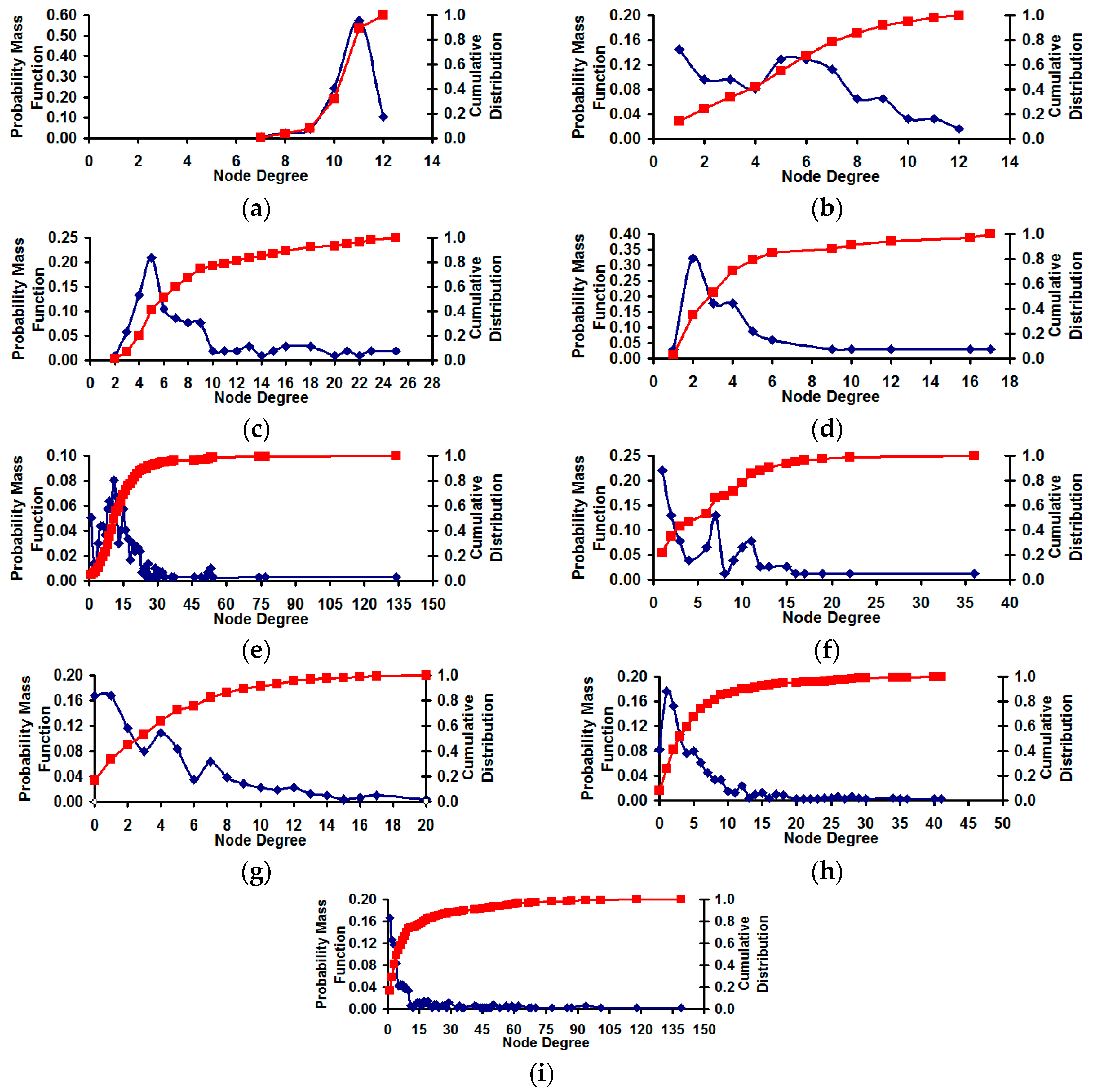
All the nine real-world networks considered are modeled as undirected network graphs. Figure 8 illustrates the degree distribution of the real-world network graphs (both the probability mass function and the cumulative distribution [24]), listed in the increasing order of the spectral radius ratio for node degree. The spectral radius ratio for node degree (denoted λsp) for a graph [25] captures the extent of variation of the node degree with respect to the average node degree and is calculated as the ratio of the principal eigenvalue of the adjacency matrix of the graph and the average node degree (denoted kavg). The value for λsp is always greater than or equal to 1.0. The farther the λsp value from 1.0, the larger the variation in node degree. The US Football Network (FN) has a λsp value of 1.01 (vindicating the Poisson-style degree distribution) and the degree distribution of the other real-world networks gradually becomes scale-free [26], with the US Airports Network (AN) having the largest λsp value of 3.22.
Figure 8.
Degree distribution of the real-world Network graphs. (a) US football network (FN): λsp = 1.01; (b) Dolphin Network (DN): λsp = 1.40; (c) US Politics Book Network (PN): λsp = 1.42; (d) Karate Network (KN): λsp = 1.47; (e) C. Elegans Network (NN): λsp = 1.68; (f) Les Miserables Network (LN): λsp = 1.82; (g) Citation GD Network (CN): λsp = 2.24; (h) Erdos971 Network (EN): λsp = 2.28; (i) US Airports Network (AN): λsp = 3.22.

We measure the following five performance metrics and the probability distribution: (i) Cumulative Modularity Score of the best possible communities detected by each of the algorithms; (ii) Execution time (in milliseconds) for each of the algorithms; (iii) Giant community size—Fraction of the nodes in the largest community among the communities detected; (iv) Resolution limit—Fraction of the communities of the smallest size among all the communities detected; (v) Normalized Mutual Information, NMI: Measure of the extent of similarity (evaluated as a quantitative score from 0 to 1) between the communities detected by two different algorithms; and (vi) Cumulative probability of finding a community of size less than or equal to a certain value. We also introduce a new metric called the MREN score (M-Modularity score; R-Resolution limit; E-Execution time; N-Number of nodes) to evaluate the effectiveness of a community detection algorithm with respect to balancing the tradeoffs among the metrics (modularity score, resolution limit and execution time). Quantitatively, the MREN score for a community detection algorithm run on a particular network is calculated as the ratio of the product of the cumulative modularity score of the communities detected and the Resolution limit to that of the product of the logarithm of the execution time (in milliseconds) and the number of nodes in the network. The inclusion of the number of nodes in the network as part of the calculation of the MREN score facilitates to make the score as a global measure of evaluating the effectiveness of a community detection algorithm. We claim that larger the MREN score (i.e., farther away the score is from 0.0), the larger the effectiveness of the algorithm with respect to balancing the tradeoffs among modularity optimization, resolution limit and execution time. In the case of the NOVER algorithm, we also measure the Threshold NOVER score for weak tie classification.
Figure 9.
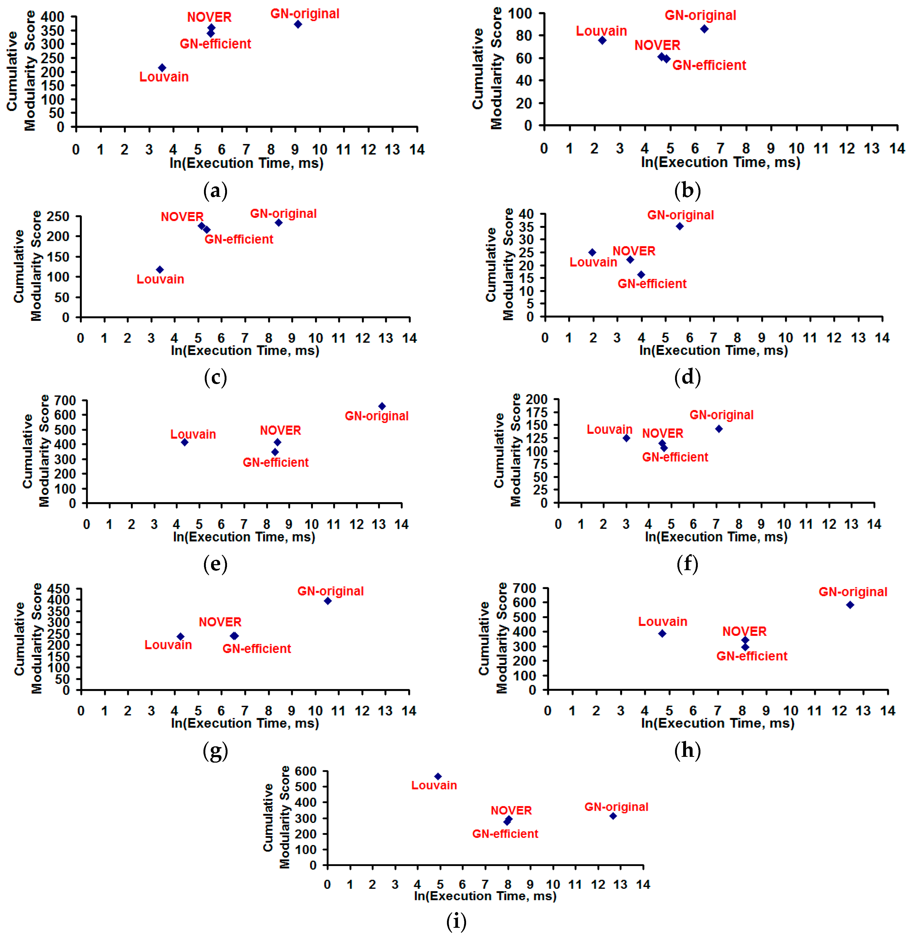
Cumulative modularity score vs. execution time for the community detection algorithms on real-world Networks graphs. (a) US FOOTBALL Network (FN); (b) Dolphin Network (DN); (c) US Politics Book Network (PN); (d) Karate Network (KN); (e) C. Elegans Network (NN); (f) Les Miserables Network (LN); (g) Citation GD Network (CN); (h) Erdos971 Collaboration Network (EN); (i) US Airports Network (AN).
Figure 9.
Cumulative modularity score vs. execution time for the community detection algorithms on real-world Networks graphs. (a) US FOOTBALL Network (FN); (b) Dolphin Network (DN); (c) US Politics Book Network (PN); (d) Karate Network (KN); (e) C. Elegans Network (NN); (f) Les Miserables Network (LN); (g) Citation GD Network (CN); (h) Erdos971 Collaboration Network (EN); (i) US Airports Network (AN).

The community detection algorithms were implemented in Java. We take into consideration only the time needed to execute all the steps of the algorithms and not the time incurred to read the network graph file (containing the node and edge information) and print the results. Hence, the execution time measured is a direct measure of the theoretical time-complexity of the algorithms as presented in Section 4. The simulations were run on a computer with Intel Core i7-2620M CPU @ 2.70 GHz and an installed memory (RAM) of 8 GB. Figure 9 and Figure 10 respectively present the values for the execution time vs. cumulative modularity score and fraction of the communities of the smallest size vs. cumulative modularity score obtained for the community detection algorithms in each of the real-world networks. Figure 11 displays the cumulative probability of finding a community of various size under each of the community detection algorithms for the real-world networks studied.
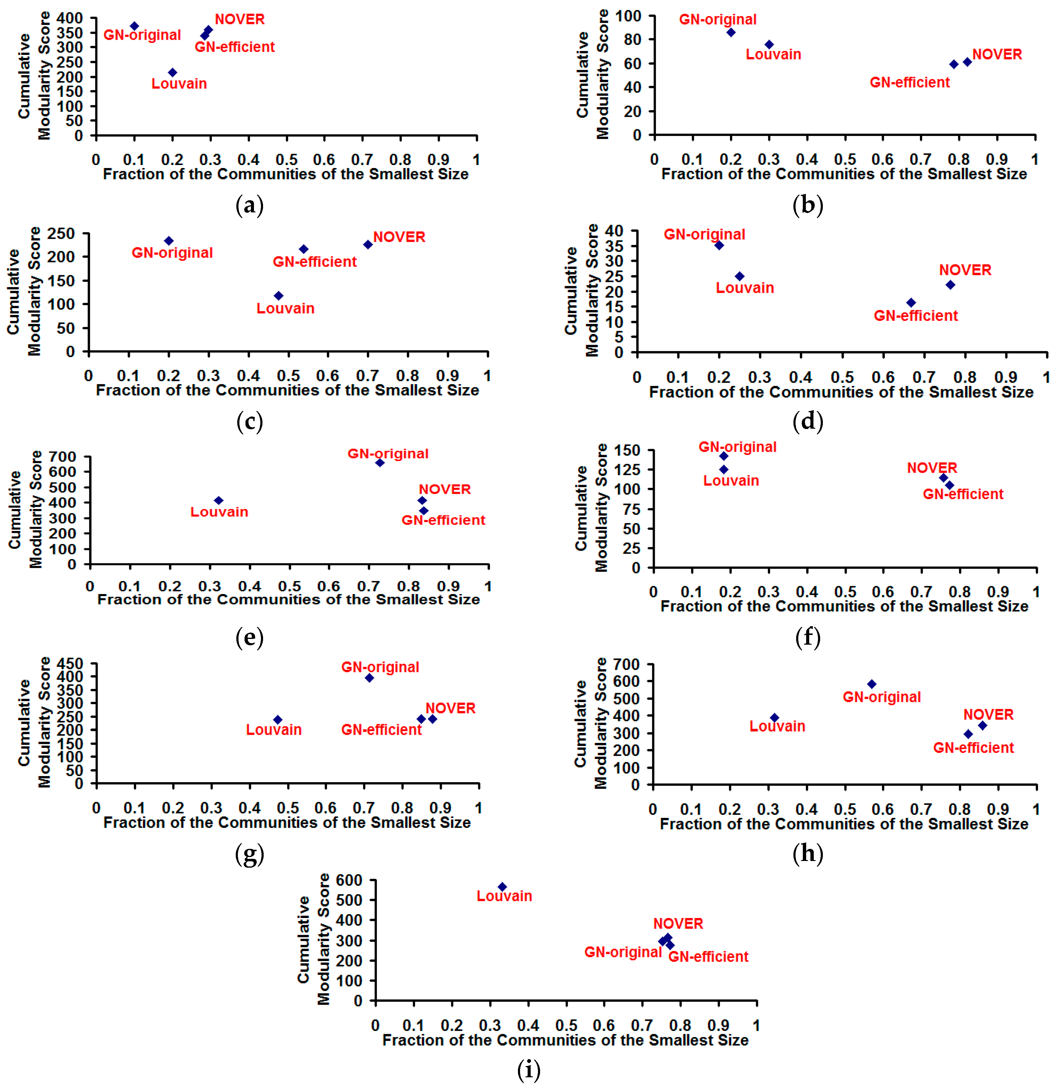
Figure 10.
Cumulative modularity score vs. fraction of the communities of the smallest size for the community detection algorithms on real-world Network graphs. (a) US Football Network (FN); (b) Dolphin Network (DN); (c) US Politics Book Network (PN); (d) Karate Network (KN); (e) C. Elegans Network (NN); (f) Les Miserables Network (LN); (g) Citation GD Network (CN); (h) Erdos971 Collaboration Network (EN); (i) US Airports Network (AN).

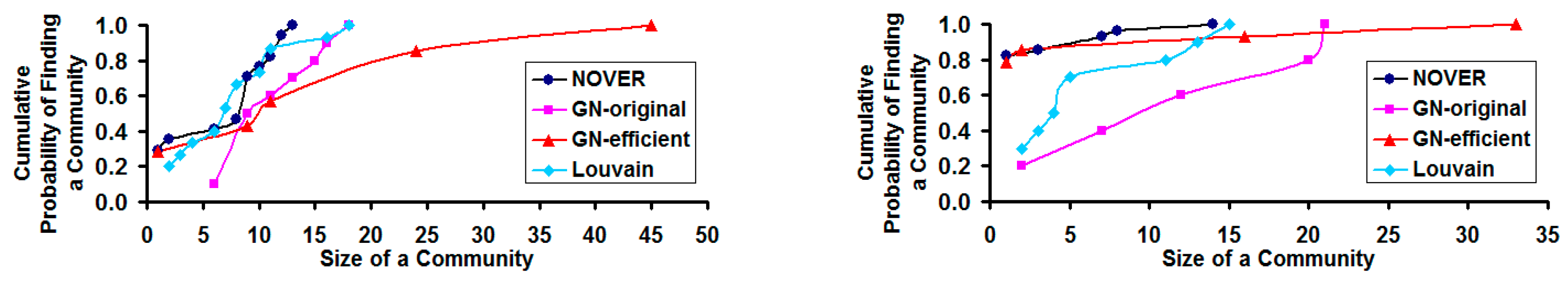
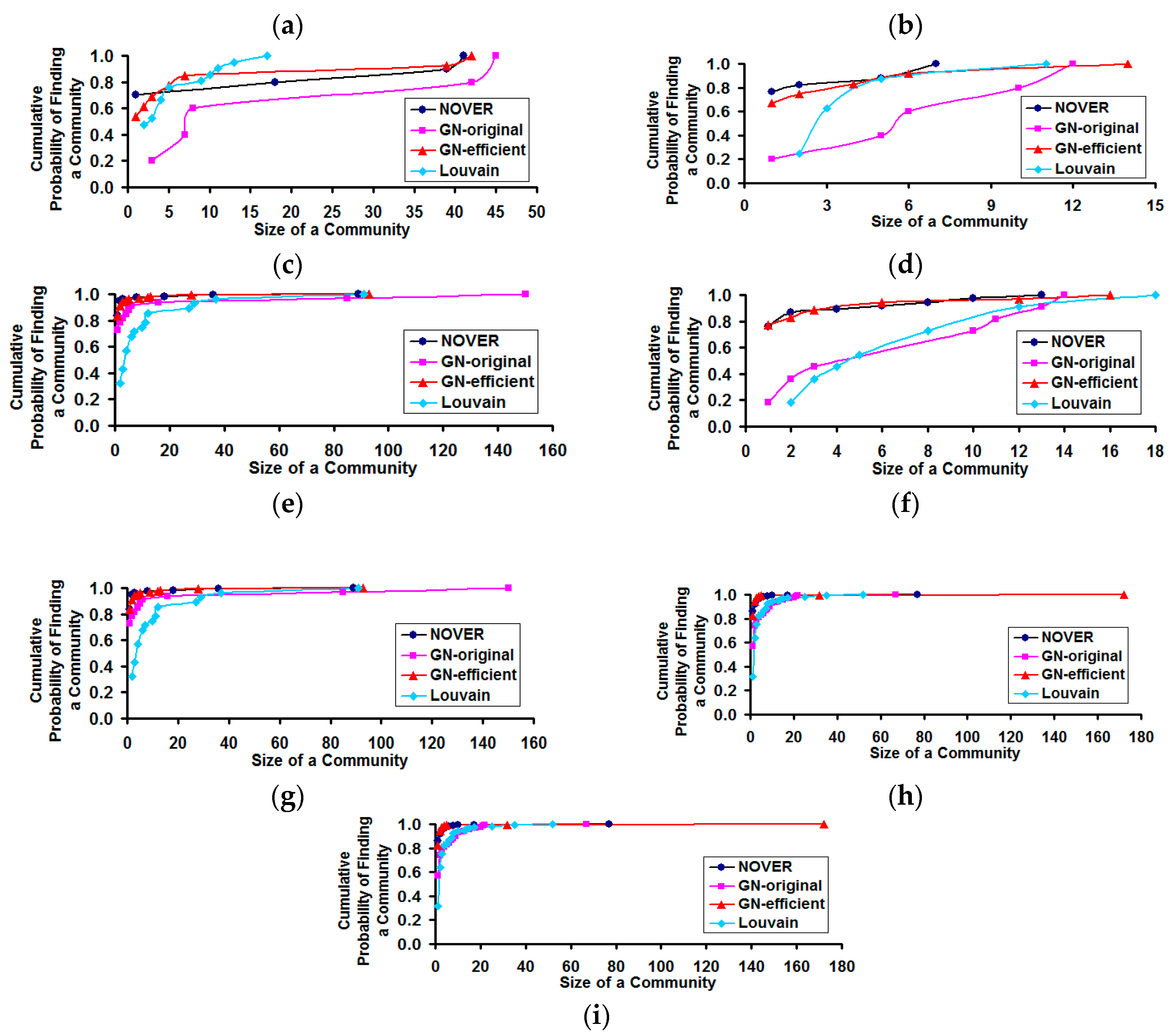
Figure 11.
Cumulative probability distribution for finding a community of certain size in real-world Network graphs. (a) US Football Network (FN); (b) Dolphin Network (DN); (c) US Politics Book Network (PN); (d) Karate Network (KN); (e) C. Elegans Network (NN); (f) Les Miserables Network (LN); (g) Citation GD Network (CN); (h) Erdos971 Collaboration Network (EN); (i) US Airports Network (AN).


The Louvain algorithm incurs the smallest execution time for all the real-world networks, as its execution time is theoretically proportional to Θ(|V| × log|V|) whereas the execution time of the GN-original algorithm is theoretically proportional to Θ(|E| × |V|(|V| + |E|)). The GN-original algorithm takes the longest execution time for all the real-world networks, but at the same time incurs the largest cumulative modularity score for eight of the nine real-world networks. The Louvain algorithm incurs the largest cumulative modularity score for only the US Airports Network. The cumulative modularity score incurred with the NOVER algorithm is significantly larger than that of the Louvain algorithm for two of the nine real-world networks (US Football network and US Politics Book network) whose spectral radius ratio for node degree is in the lower range (λsp ≤ 1.5). For five of the nine real-world networks, the NOVER algorithm incurs a cumulative modularity score that is very much comparable to that of the Louvain algorithm. Only for the US Airports network and Dolphin network, we observe the cumulative modularity score of the Louvain algorithm to be appreciably larger than that of the NOVER algorithm. All of the above observations hold true with the execution time of the NOVER algorithm significantly lower to that of the GN-original algorithm; the difference in execution time increases with increase in the number of nodes and/or the number of edges. The GN-original algorithm is significantly slower for networks with a larger number of nodes and/or edges. The NOVER algorithm incurs an execution time that is either less than or at most equal to that of the GN-efficient algorithm for all the real-world networks, and at the same time incurs a cumulative modularity score that is always either larger or at the worst case equal to that of the GN-efficient algorithm; note that both the NOVER and GN-efficient algorithms have the same theoretical time-complexity of Θ(|E| × (|V| + |E|)).
Figure 12.
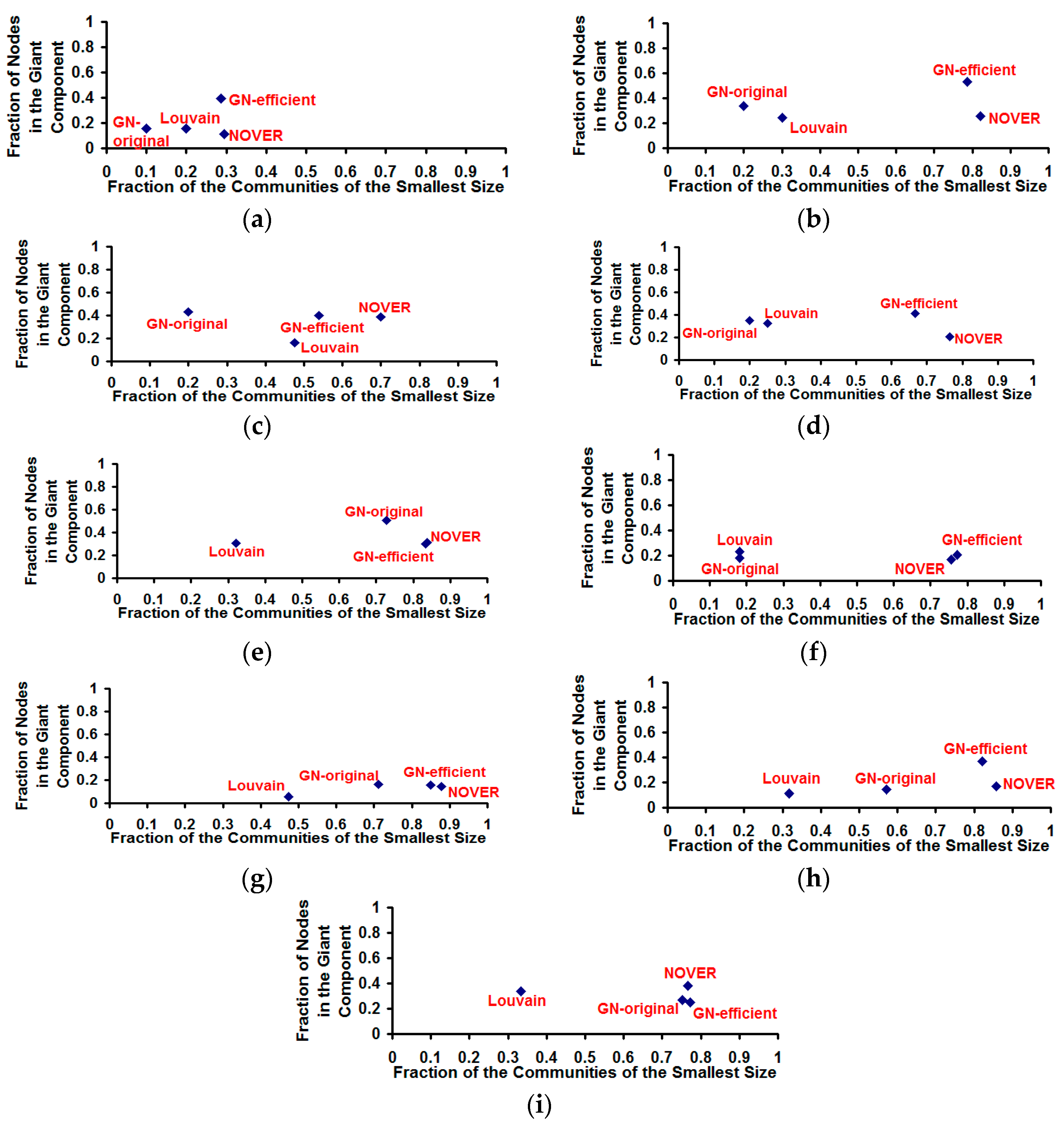
Fraction of nodes in the giant component vs. fraction of the communities of the smallest size for the community detection algorithms on real-world Network graphs. (a) US Football Network (FN); (b) Dolphin Network (DN); (c) US Politics Book Network (PN); (d) Karate Network (KN); (e) C. Elegans Network (NN); (f) Les Miserables Network (LN); (g) Citation GD Network (CN); (h) Erdos971 Collaboration Network (EN); (i) US Airports Network (AN).
Figure 12.
Fraction of nodes in the giant component vs. fraction of the communities of the smallest size for the community detection algorithms on real-world Network graphs. (a) US Football Network (FN); (b) Dolphin Network (DN); (c) US Politics Book Network (PN); (d) Karate Network (KN); (e) C. Elegans Network (NN); (f) Les Miserables Network (LN); (g) Citation GD Network (CN); (h) Erdos971 Collaboration Network (EN); (i) US Airports Network (AN).

Though the Louvain algorithm and GN-original algorithm appear to be respectively optimal incurring the lowest execution time and largest cumulative modularity score, we observe both these algorithms suffer from the poor resolution problem (incur lower values for the fraction of communities of smaller size), especially the Louvain algorithm. Due to the multi-level aggregation nature of the Louvain algorithm, it becomes difficult to detect communities of size lower than a certain value that could indeed contribute to a larger cumulative modularity score. On the other hand, the NOVER algorithm is able to detect communities of smaller size with an appreciably higher probability and at the same time incurs a larger cumulative modularity score that is very much comparable to that of the Louvain algorithm for seven of the nine real-world networks. Though the GN-efficient algorithm incurs a comparable value (to that of the NOVER algorithm) for the resolution limit for most of the real-world networks, there exists at least a couple of real-world networks for which the fraction of communities of smallest size detected by the GN-efficient algorithm is lower than that of the NOVER algorithm.
With respect to the cumulative probability distribution of the community size (see Figure 11), we observe the community size distribution to follow a power-law pattern, similar to that of the degree distribution. We observe the NOVER algorithm to incur a larger probability of finding a community of smaller to moderate size for real-world networks with lower variation in node degree (i.e., spectral radius ratio for node degree ≤1.5). As the spectral radius ratio for node degree increases beyond 1.5, we observe the cumulative probability distribution profiles for the community sizes detected by all the community detection algorithms to overlap with each other. For networks of moderate variation in node degree, the GN-original and Louvain algorithms appear to sustain a relatively lower cumulative probability for finding a community of size less than or equal to a certain value.
The original and time-efficient versions of the Girvan-Newman algorithm appear to detect giant components of relatively larger size (see Figure 12) compared to that of the Louvain and NOVER algorithms. The GN-efficient algorithm detects communities with a larger resolution limit (fraction of the communities of the smallest size) as well as a larger giant component size (fraction of the nodes in the largest community) for most of the real-world networks. The NOVER algorithm also accomplishes a larger resolution limit that is very much comparable to that of the GN-efficient algorithm, but the giant component size falls short of the GN-efficient algorithm. Nevertheless, the NOVER algorithm detects giant components of relatively larger size than that of the Louvain algorithm for five of the nine real-world networks analyzed. Additionally, we did not observe any ties for the giant component; all the community detection algorithms detected only one single giant component of the largest size on each of the real-world network graphs; on the other hand, there existed several communities of the smallest size in the case of each of the algorithms.
In addition to the modularity score, we also quantitatively compare the NOVER algorithm with the other three algorithms based on a commonly used information-theoretic measure called the Normalized Mutual Information (NMI) score [12]. The NMI score (0 ... 1) is a quantitative measure of the extent of similarity between the communities detected by any two community detection algorithms. Let CA and CB be the sets of communities (identified respectively with indexes a = 1, ..., |CA| and b = 1, ..., |CB|) detected by two different community detection algorithms A and B on a network graph of n nodes; let , , be, respectively, the number of vertices in the community of index a detected by algorithm A, the number of vertices in the community of index b detected by algorithm B and the number of common vertices in the communities of indexes a and b detected by algorithms A and B; then the NMI score for the two algorithms is given by the following formulation:
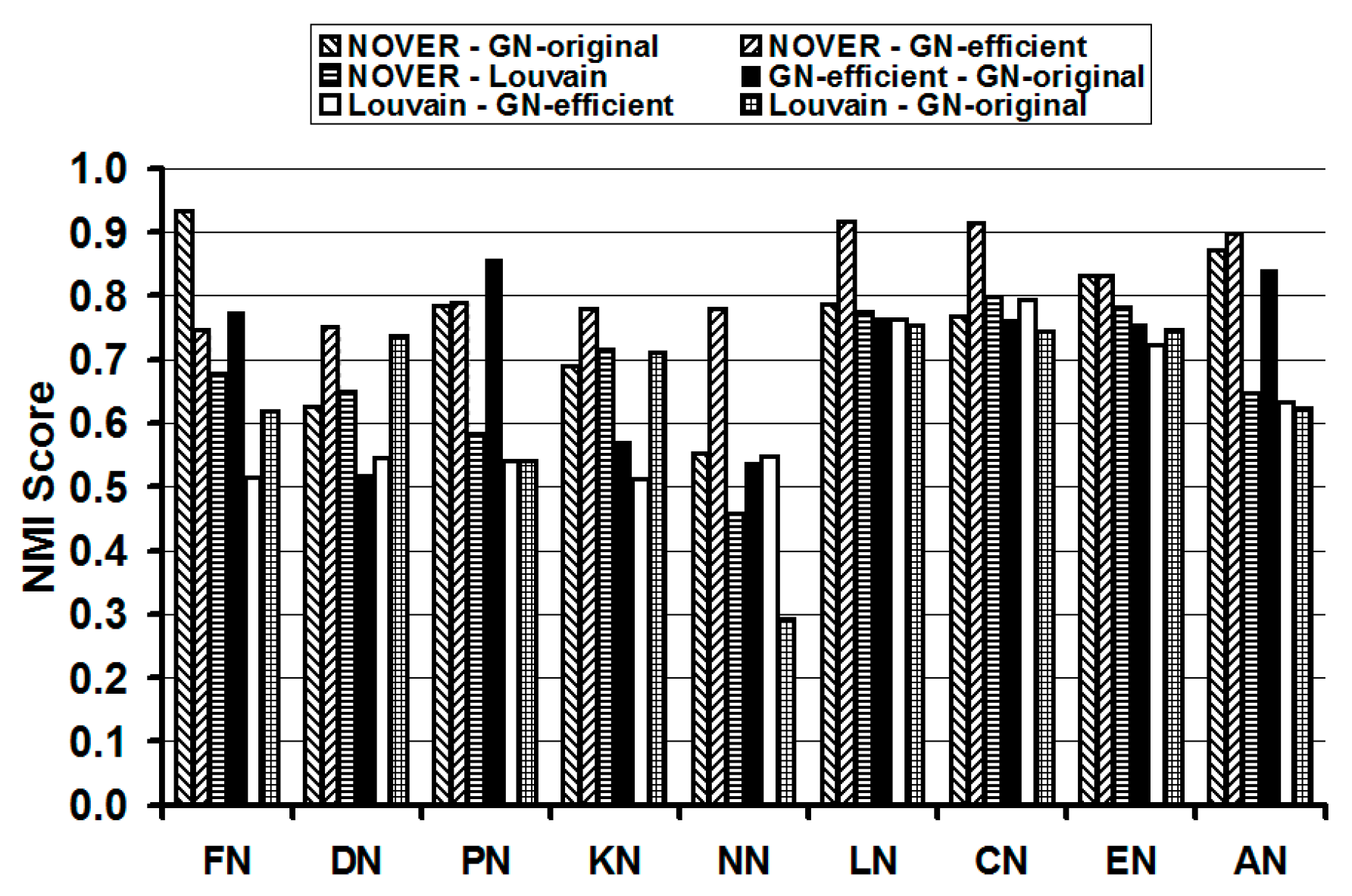
We use the NMI score as the basis to compare the relative similarity of the communities detected by any two of the four community detection algorithms on each of the nine real-world networks studied in this paper. If the sets of communities detected by two different community detection algorithms are identical, then the NMI score of the two algorithms is 1. Thus, larger the NMI score of two community detection algorithms, the larger is the similarity in the composition of the communities detected by the two algorithms. The results are displayed in Table 1 and pictorially illustrated in Figure 13. We color code (the cells in Table 1 are shaded in gray) the cells corresponding to the pairs of community detection algorithms incurring the top three NMI scores for each real-world network. We observe the NOVER algorithm mutually evaluated with each of the GN-original, GN-efficient and Louvain algorithms to be part of at least two of the top three combinations of the community detection algorithms with larger NMI scores. The NMI values of the NOVER algorithm with each of the other three algorithms are 0.75 or above in 18 of the 27 cells in Table 1. This indicates that the composition of the communities detected by NOVER algorithm is not vastly different from that of the communities detected by the other three algorithms; but these communities are detected at a much lower execution time (compared to that of the GN-original algorithm) as well as at a relatively higher resolution limit (especially when compared to the communities detected by the Louvain algorithm). The NMI scores of the NOVER-Louvain algorithms are lower than those observed for the NOVER-GN-efficient and NOVER-GN-original algorithms. On this basis, we could say that the composition of the communities detected by NOVER algorithm is relatively more different from that of the Louvain algorithm vis-à-vis the composition of communities detected by the GN-original and GN-efficient algorithms. For all the nine real-world networks, the NMI scores incurred for NOVER when compared with the GN-efficient algorithm is 0.75 or above. Such a high-level of similarity in the composition of the communities detected by the NOVER and GN-efficient algorithms is also observed in the results displayed in Figure 9, Figure 10, Figure 11 and Figure 12.
Figure 13.
Illustration of the mutual comparison of the community detection algorithms on real-world Network graphs based on NMI scores.
Figure 13.
Illustration of the mutual comparison of the community detection algorithms on real-world Network graphs based on NMI scores.


| Network Abbreviation | NOVER-GN-Original | NOVER-GN-Efficient | NOVER-Louvain | GN-Efficient-GN-Original | Louvain-GN-Efficient | Louvain-GN-Original |
|---|---|---|---|---|---|---|
| FN | 0.934 | 0.756 | 0.677 | 0.775 | 0.516 | 0.618 |
| DN | 0.626 | 0.751 | 0.649 | 0.519 | 0.545 | 0.737 |
| PN | 0.785 | 0.789 | 0.583 | 0.859 | 0.541 | 0.540 |
| KN | 0.690 | 0.781 | 0.716 | 0.572 | 0.513 | 0.712 |
| NN | 0.552 | 0.781 | 0.459 | 0.538 | 0.547 | 0.293 |
| LN | 0.786 | 0.918 | 0.776 | 0.766 | 0.763 | 0.754 |
| CN | 0.768 | 0.914 | 0.799 | 0.764 | 0.794 | 0.745 |
| EN | 0.831 | 0.832 | 0.782 | 0.755 | 0.724 | 0.746 |
| AN | 0.873 | 0.899 | 0.647 | 0.841 | 0.633 | 0.624 |
We observe the NOVER algorithm to effectively balance the performance tradeoffs with respect to the cumulative modularity score, execution time and resolution limit. In this pursuit, we observe the MREN score (see Figure 14) for the NOVER algorithm to be appreciably larger than that of the other three community detection algorithms for eight of the nine real-world networks, except the airport network. The GN-original algorithm incurs the lowest MREN score for eight of the nine real-world networks, except the C. Elegans Neural network (for which we observe the Louvain algorithm to sustain a lower MREN score), attributed to its significantly larger execution time. We propose the MREN score to be a performance measure that is independent of the node size so that we can capture the effectiveness of the community detection algorithms on a comparable globally common scale. For example, in Figure 14, we observe the MREN scores of the community detection algorithms for the Karate network and the US Airport network to be comparable to each other (even though the two networks are of significantly different sizes).
Figure 14.
Comparison of the MREN scores of the community detection algorithms on real-world Network graphs.
Figure 14.
Comparison of the MREN scores of the community detection algorithms on real-world Network graphs.

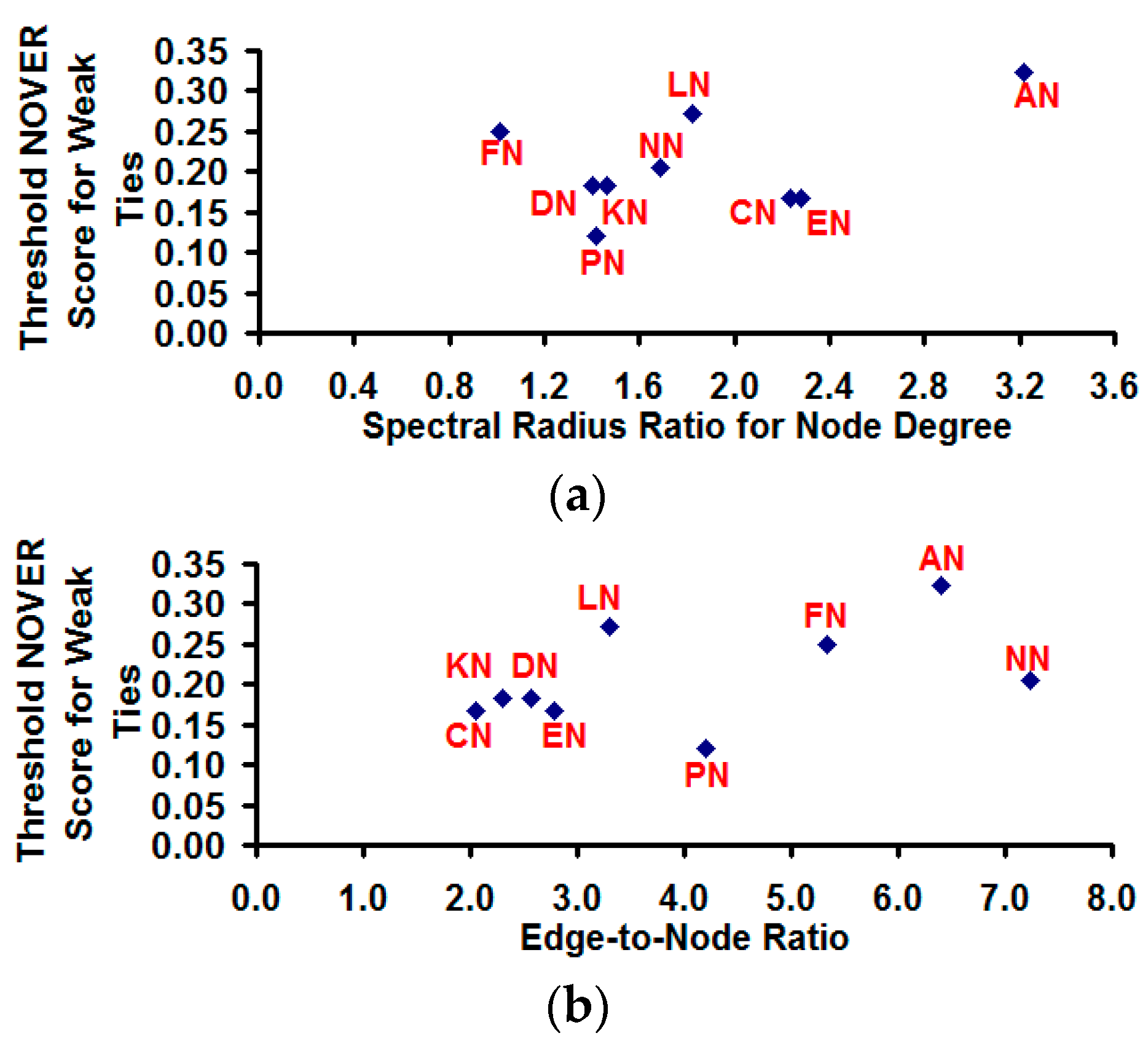
With regards to the threshold NOVER score for community partition, we observe our hypothesis in Section 2 to be indeed true: i.e., the threshold NOVER score for classification of edges as weak ties and strong ties for detecting highly modular communities cannot be arbitrarily chosen, and an appropriate value for the threshold NOVER score appears to somewhat depend on the variation in node degree of the vertices as well as on the edge-to-node ratio (see Figure 15). The overall trend we observe is that the threshold NOVER score is more likely to increase with increase in the spectral radius ratio for node degree (correlation coefficient: 0.44) and with increase in the edge-to-node ratio (correlation coefficient: 0.49).
Figure 15.
Dependence of the threshold NOVER score for weak ties on the spectral radius ratio for node degree and the edge-to-node ratio. (a) Spectral radius ratio for node degree vs. Threshold NOVER score for weak ties; (b) Edge-to-node ratio vs. Threshold NOVER score for weak ties.
Figure 15.
Dependence of the threshold NOVER score for weak ties on the spectral radius ratio for node degree and the edge-to-node ratio. (a) Spectral radius ratio for node degree vs. Threshold NOVER score for weak ties; (b) Edge-to-node ratio vs. Threshold NOVER score for weak ties.

6. Related Work
In this section, we review the related work available in the literature with regards to the use of neighborhood information and edge betweenness for community detection. The importance of using weak ties to analyze relations between disparate groups emanated from the classical work of Granovetter [27] in which it was observed that the strength of the relationship between any two users in a social network increased with increase in the number of common neighbors. In [13], it was observed that the NOVER scores of edges (as defined in this paper) connecting two different communities is significantly lower than the NOVER scores of edges within each community. However, the work done in [13] was just an analytical study of the Facebook network: the NOVER scores were merely computed for the edges and not used as part of a formal algorithm for community detection. Further, as an experimental study, it was stated in [28] that the average talk time of two users in a telephone network increases with increase in the number of common friends for the two users. All of these support our hypothesis for using edges with low neighborhood overlap as the basis of community detection. If two users had several common neighbors and had a higher neighborhood overlap, then the two users as well as their neighbors belong to one single tightly-knit community. On the other hand, if an edge connecting two users with a lower neighborhood overlap score is removed, it could potentially disconnect the two neighbors from further communication—Indicating that the two nodes belong to two different communities that have relatively fewer edges crossing the two communities, compared to the number of edges within the individual communities.
In [29], the authors proposed an iterative and hierarchical community detection algorithm that makes use of the neighborhood overlap information of the edges; the idea is to assign each node to a community with which it has strong average aggregated link strength compared to the other communities. Two primary weaknesses of this algorithm are that it partitions a community (to start with all the vertices in the graph are considered to be in one community) into only two communities at a time (irrespective of the modular nature of the network) and assigns the nodes from the original community to one of the two partitions; further the algorithm requires the selection of an appropriate value of a control parameter to stop the partitioning of a community into two communities. On the other hand, our proposed NOVER algorithm does not require the use of any control parameter for its operation; the edges are simply removed in the increasing order of their NOVER values and we observe such a greedy strategy (running at a significantly lower computation time) pays rich dividends by incurring cumulative modularity scores that are only at most 60% of those determined by the Girvan-Newman algorithm for optimal community detection.
With regards to the use of edge betweenness for community detection, several algorithms have been proposed in the literature to detect highly modular communities at a relatively smaller computation time compared to the original Girvan-Newman algorithm for community detection. We discuss some of these algorithms here: In [10], the authors fix the number of targeted communities (K) in a network of N nodes; nodes associated with edges whose betweenness values are lower than (N/K) × β (where 0 < β ≤ 1 is a control parameter) are grouped within a community. Tyler et al. [8] suggest to run the BFS algorithm on a sample of the vertices (randomly chosen for each iteration) for each edge removal, instead of running the BFS algorithm on all the vertices of the graph in each iteration. Since, we are interested in identifying only the edge with the largest betweenness to be removed in each iteration, the assumption behind the work in [8] is that as long as the number of samples is sufficiently large, the error introduced due to the random sampling will not make a significant impact on the quality of the partitioning. Radichhi et al. [9] observed an inverse correlation between a measure called the edge clustering coefficient and the edge betweenness. The clustering coefficient of an edge (as defined in [9]) is the ratio of the number of triangles to which the edge belongs to that of the number of triangles that might potentially include it, given the degrees of the adjacent nodes. An edge that has a lower clustering coefficient is likely to be between two communities and an edge that has a higher clustering coefficient is likely to be well-knit within a community. Radicchi et al. [9] advocate the removal of an edge with the smallest clustering coefficient per iteration and recalculating the edge clustering coefficient values for each iteration; this is expected to be not that time consuming as that of the procedure to re-compute the edge betweenness values for each iteration.
7. Conclusions and Future Work
We observe the NOVER algorithm to incur a cumulative modularity score that is larger than that of the GN-efficient algorithm as well as incurs a significantly lower execution time compared to that of the GN-original algorithm. The NOVER algorithm also incurs a comparable modularity score to that of the Louvain algorithm. Though the Louvain algorithm incurs a relatively lower execution time, the NOVER algorithm has been observed to effectively balance the tradeoffs between modularity optimization, execution time and resolution limit (fraction of communities of the smallest size) and incur the largest MREN score for eight of the nine real-world networks analyzed. On the basis of the NMI scores, it appears that the composition of the communities detected by the NOVER algorithm is relatively more closer to that of the GN-efficient and GN-original algorithms, compared to that of the Louvain algorithm. Nevertheless, the composition of the communities detected by the NOVER algorithm appears to be not significantly different from that of the other algorithms (on the basis of the NMI scores). The MREN score proposed in this paper could serve as a global measure (independent of the network size) for evaluating the effectiveness of a community detection algorithm. Both the GN-Efficient and NOVER algorithms adopt a similar design strategy of using an edge measure that is only calculated once (on the input graph itself) and using these initial values of the edge measure to remove the edges (one edge per iteration). The GN-Efficient algorithm removes the edges in the decreasing order of their betweenness values, while the NOVER algorithm removes the edges in the increasing order of their neighborhood overlap values. We observe the NOVER algorithm to provide a higher dividend and detect communities whose cumulative modularity score is relatively larger than that of the communities detected using the GN-efficient algorithm and more closer to the cumulative modularity score of the communities detected using the GN-original algorithm. Thus, the NOVER algorithm is a valuable addition to the literature for community detection and is worth to be investigated for further optimization. As part of future work, we plan to incorporate optimizations (for example: merging of the one-vertex communities) to effectively run the NOVER algorithm for scale-free networks with lower edge-to-node ratio. We plan to compare the performance of the improved NOVER algorithm with that of several edge betweenness-based community detection algorithms (in addition to the Girvan-Newman algorithm).
Acknowledgments
This work is partly funded through the NASA-EPSCoR sub award (# NNX14AN38A) from University of Mississippi.
Conflicts of Interest
The author declares no conflict of interest.
References
- Fortunato, S. Community Detection in Graphs. Phys. Rep. 2010, 486, 75–174. [Google Scholar] [CrossRef]
- Newman, M.E.J. Modularity and Community Structure in Networks. J. Natl. Acad. Sci. USA 2006, 103, 8557–8582. [Google Scholar] [CrossRef] [PubMed]
- Brandes, U.; Delling, D.; Gaertler, M.; Gorke, R.; Hoefer, M.; Nikoloski, Z.; Wagner, D. On Modularity Clustering. IEEE Trans. Knowl. Data Eng. 2008, 20, 172–188. [Google Scholar] [CrossRef]
- Girvan, M.; Newman, M.E. Community Structure in Social and Biological Networks. J. Natl. Acad. Sci. USA 2002, 99, 7821–7826. [Google Scholar] [CrossRef] [PubMed]
- Newman, M.E.J. Detecting Community Structure in Networks. Eur. Phys. J. B Condens. Matter Complex Syst. 2004, 38, 321–330. [Google Scholar] [CrossRef]
- Fortunato, S.; Barthelemy, M. Resolution Limit in Community Detection. J. Natl. Acad. Sci. USA 2007, 104, 36–41. [Google Scholar] [CrossRef] [PubMed]
- Blondel, V.D.; Guillaume, J.-L.; Lambiotte, R.; Lefebvre, E. Fast Unfolding of Communities in Large Networks. J. Stat. Mech. Theory Exp. 2008, P10008, 1–11. [Google Scholar] [CrossRef]
- Tyler, J.R.; Wilkinson, D.M.; Huberman, B.A. Email as Spectroscopy: Automated Discovery of Community Structure within Organizations. Inform. Soc. Int. J. 2007, 21, 143–153. [Google Scholar] [CrossRef]
- Radicchi, F.; Castellani, C.; Cecconi, F.; Loreto, V.; Parisi, D. Defining and Identifying Communities in Networks. J. Natl. Acad. Sci. USA 2004, 101, 2658–2663. [Google Scholar] [CrossRef] [PubMed]
- Luo, T.; Zhong, C.; Ying, X.; Fu, J. Detecting Community Structure based on Edge Betweenness. In Proceedings of the 8th International Conference on Fuzzy Systems and Knowledge Discovery, Shanghai, China, 26–28 July 2011; pp. 1133–1136.
- Easley, D.; Kleinberg, J. Networks, Crowds, and Markets: Reasoning about a Highly Connected World, 1st ed.; Cambridge University Press: Cambridge, UK, 2010. [Google Scholar]
- Ana, L.N.F.; Jain, A.K. Robust Data Clustering. In Proceedings of the IEEE Conference on Computer Vision and Pattern Recognition, Madison, WI, USA, 16–22 June 2003; pp. 128–133.
- De Meo, P.; Ferrara, E.; Fiumara, G.; Provetti, A. On Facebook, Most Ties Are Weak. Commun. ACM 2014, 57, 78–84. [Google Scholar] [CrossRef]
- Lancichinetti, A.; Fortunato, S. Limits of Modularity Maximization in Community Detection. Phys. Rev. E 2011, 84, 066122. [Google Scholar] [CrossRef] [PubMed]
- Erciyes, K. Complex Networks: An Algorithmic Perspective, 1st ed.; CRC Press: Boca Raton, FL, USA, 2014. [Google Scholar]
- Lusseau, D.; Schneider, K.; Boisseau, O.J.; Haase, P.; Slooten, E.; Dawson, S.M. The Bottlenose Dolphin Community of Doubtful Sound Features a Large Proportion of Long-Lasting Associations. Behav. Ecol. Sociobiol. 2003, 54, 396–405. [Google Scholar] [CrossRef]
- Zachary, W.W. An Information Flow Model for Conflict and Fission in Small Groups. J. Anthropol. Res. 1977, 33, 452–473. [Google Scholar]
- Krebs, V. Book Networks. Int. Assoc. Hum. Resour. Inform. Manag. J. 2000, 4, 87–90. [Google Scholar]
- Jia, T.; Qin, K.; Shan, J. An Exploratory Analysis on the Evolution of the US AIrport Network. Phys. A Stat. Mech. Appl. 2014, 413, 266–279. [Google Scholar] [CrossRef]
- Batagelj, V.; Mrvar, A. Some Analyses of Erdos Collaboration Graph. Soc. Netw. 2000, 22, 173–186. [Google Scholar] [CrossRef]
- Knuth, D.E. The Stanford GraphBase: A Platform for Combinatorial Computing, 1st ed.; Addison-Wesley: Boston, MA, USA, 1993. [Google Scholar]
- Cangelosi, A.; Parisi, D. A Neural Network Model of Caenorhabditis Elegans: The Circuit of Touch Sensitivity. Neural Process. Lett. 1997, 6, 91–98. [Google Scholar] [CrossRef]
- Biedl, T.; Brandenburg, F. Graph-Drawing Contest Report. In Proceedings of the 9th International Symposium on Graph Drawing, Vienna, Austria, 23–26 September 2001; pp. 82–85.
- Ross, S.M. Introduction to Probability Models, 11th ed.; Academic Press: Cambridge, MA, USA, 2014. [Google Scholar]
- Meghanathan, N. Spectral Radius as a Measure of Variation in Node Degree for Complex Network Graphs. In Proceedings of the 7th International Conference on u- and e-Service, Science and Technology, Haikou, China, 20–23 December 2014; pp. 30–33.
- Barabasi, A.-L.; Albert, R. Emergence of Scaling in Random Networks. Science 1999, 286, 509–512. [Google Scholar] [PubMed]
- Granovetter, M.S. The Strength of Weak Ties. Am. J. Sociol. 1973, 78, 1360–1380. [Google Scholar] [CrossRef]
- Onnela, J.-P.; Saramaki, J.; Hyvonven, J.; Szabo, G.; Lazer, D.; Kaski, K.; Kertesz, J.; Barabasi, A.-L. Structure and Tie Strengths in Mobile Communication Networks. J. Natl. Acad. Sci. USA 2007, 104, 7332–7336. [Google Scholar] [CrossRef] [PubMed]
- Li, K.; Gong, X.; Guan, S.; Lai, C.-H. Efficient Algorithm Based on Neighborhood Overlap for Community Identification in Complex Networks. Phys. A Stat. Mech. Appl. 2012, 391, 1788–1796. [Google Scholar] [CrossRef]
© 2016 by the author; licensee MDPI, Basel, Switzerland. This article is an open access article distributed under the terms and conditions of the Creative Commons by Attribution (CC-BY) license (http://creativecommons.org/licenses/by/4.0/).
Share and Cite
MDPI and ACS Style
Meghanathan, N. A Greedy Algorithm for Neighborhood Overlap-Based Community Detection. Algorithms 2016, 9, 8. https://0-doi-org.brum.beds.ac.uk/10.3390/a9010008
AMA Style
Meghanathan N. A Greedy Algorithm for Neighborhood Overlap-Based Community Detection. Algorithms. 2016; 9(1):8. https://0-doi-org.brum.beds.ac.uk/10.3390/a9010008
Chicago/Turabian StyleMeghanathan, Natarajan. 2016. "A Greedy Algorithm for Neighborhood Overlap-Based Community Detection" Algorithms 9, no. 1: 8. https://0-doi-org.brum.beds.ac.uk/10.3390/a9010008
Note that from the first issue of 2016, this journal uses article numbers instead of page numbers. See further details here.