Application of Machine Learning in Evaluation of the Static Young’s Modulus for Sandstone Formations


College of Petroleum Engineering and Geosciences, King Fahd University of Petroleum & Minerals, Dhahran 31261, Saudi Arabia
*
Author to whom correspondence should be addressed.
Sustainability 2020, 12(5), 1880; https://0-doi-org.brum.beds.ac.uk/10.3390/su12051880
Submission received: 17 January 2020
/
Revised: 26 February 2020
/
Accepted: 28 February 2020
/
Published: 2 March 2020
(This article belongs to the Special Issue Artificial Intelligence and Cognitive Computing: Methods, Technologies, Systems, Applications and Policy Making)
Abstract
:Prediction of the mechanical characteristics of the reservoir formations, such as static Young’s modulus (Estatic), is very important for the evaluation of the wellbore stability and development of the earth geomechanical model. Estatic considerably varies with the change in the lithology. Therefore, a robust model for Estatic prediction is needed. In this study, the predictability of Estatic for sandstone formation using four machine learning models was evaluated. The design parameters of the machine learning models were optimized to improve their predictability. The machine learning models were trained to estimate Estatic based on bulk formation density, compressional transit time, and shear transit time. The machine learning models were trained and tested using 592 well log data points and their corresponding core-derived Estatic values collected from one sandstone formation in well-A and then validated on 38 data points collected from a sandstone formation in well-B. Among the machine learning models developed in this work, Mamdani fuzzy interference system was the highly accurate model to predict Estatic for the validation data with an average absolute percentage error of only 1.56% and R of 0.999. The developed static Young’s modulus prediction models could help the new generation to characterize the formation rock with less cost and safe operation.
1. Introduction
Prediction of the mechanical characteristics of the reservoir formations, such as Young’s modulus (E), is necessary for the evaluation of the wellbore stability, reservoir compaction, hydraulic fracturing, and formation control [1]. E is a mechanical parameter that gives an indication of the resistance of the rock samples when exposed to a uniaxial load [2]. On the other hand, static Young’s modulus (Estatic) is a critical parameter needed to build the earth geomechanical model [3]. It is also used for fractures’ designing and mapping [4,5]. While drilling hydrocarbon wells, Estatic is also needed with other mechanical and petrophysical properties to make a full description of the in-situ stresses to ensure wellbore stability [6].
Estatic varies significantly with the change in lithology [2,7]. Estatic for shale ranges from 0.69 to 6.89 GPa. For limestone, it is between 55.16 and 82.74 GPa, and for sandstone, it is between 13.79 and 68.95 GPa [7]. These ranges confirm the wide difference in Estatic from one formation type to another and the huge change within the same lithology. Therefore, it is necessary to estimate Estatic along the whole drilled hydrocarbon well.
Two methods for rock elastic parameters’ estimation are currently available. These are the experimental laboratory method or the use of empirical correlations. The experimental laboratory method is based on conducting laboratory experiments on the rock samples using static or dynamic testing techniques. In the static technique, the sample is subjected to a uniaxial or triaxial load and the deformation of the sample is measured, while in the dynamic technique, shear and compressional wave velocities along the tested sample are measured and then the sample’s elastic parameters are calculated based on the shear wave (Vs) and compressional wave (Vp) velocity [8]. In the field, wireline logging tools are used to measure Vs and Vp. The dynamic Young’s modulus (Edynamic) can then be evaluated based on Vs and Vp and using Equation (1).
where denotes the formation’s bulk density in g/cm3, VS and VP are in km/s, and Edynamic is in GPa.
Several previous studies confirmed that the laboratory-measured Edynamic for the same rock sample is significantly greater than Estatic [9,10,11]. Edynamic could be 1.5 to 3 times greater than Estatic [12] and some recent studies reported that Edynamic could be ten times greater than Estatic [13,14]. The strain amplitude between the two experimentally testing methods is the main reason for this huge difference, which decreases as the rock strength increase [15].
The static elastic parameters are actually representative of the in-situ stress–strain conditions of the reservoir [16]. Accurate determination of the static elastic parameters requires conducting a time consuming and costly experimental tests on real core samples [17]. The common practice to decrease this high cost is to select core samples at specific intervals and conduct the experimental tests of these cores only. Then an empirical correlation between the laboratory-derived parameters and the conventional well log data will be developed based on the results of laboratory tests. The static moduli throughout the whole reservoir depths can then be predicted by calibrating the dynamic moduli using the developed correlations [4]. Because of the heterogeneity of the reservoir formations, the developed well log-based empirical equations are usually not generalized to all formation types. Therefore, different correlations need to be developed for every formation type to track the changes in the static parameters along the whole reservoir.
The correlation in Equation (2) was developed by Fei et al. [18] for the evaluation of Estatic for sandstone formations; this correlation evaluates Estatic as a function of Edynamic, which was developed based on 22 triaxial tests results.
where Estatic and Edynamic are in GPa.
Mahmoud et al. [19] developed a set of equations to estimate Estatic for different types of formations. The main advantage of the correlations developed by Mahmoud et al. [19] is the ability to implement these correlations directly to evaluate Estatic without the need for Edynamic, these correlations are only a function of the bulk formation density (RHOB), compressional transit time (DTc), and shear transit time data (DTs).
Different recent studies confirmed the ability of machine learning techniques to accurately estimate rock mechanical properties. Abdulraheem et al. [20] optimized three machine learning models of the artificial neural networks (ANN), fuzzy logic model, and functional neural networks (FNN) for estimation of Estatic and the static Poison’s ratio for the hydrocarbon reservoirs. The authors did not specify the reservoir rock formation type. The developed models confirmed their ability to estimate the reservoir rock mechanical properties.
In another study, Tariq et al. [21] developed three machine learning models of ANN, fuzzy logic, and support vector machine (SVM) to estimate Estatic for limestone formation. The ANN model overperformed the other machine learning models and the currently available empirical correlation for Estatic estimation.
Tariq et al. [22] developed empirical correlations for the estimation of the mechanical properties of Estatic, Poisson’s ratio, and unconfined compressive strength based on the application of the artificial neural networks (ANN) and the use of the conventional well log data, the authors also did not specify the type of the formation they used in this study. The developed correlations improved their ability to accurately estimate the rock mechanical properties.
In 2017, Parapuram et al. [23] developed an ANN model to estimate the geomechanical properties of the upper Bakken shale based on well log data. The results of this study confirmed the ability of the ANN model to accurately estimate the rock mechanical properties.
Recently, in our previous study, Mahmoud et al. [24], we evaluated the use of the ANN in estimating Estatic for sandstone formations. Mahmoud et al. [24] reported that ANN is able to predict Estatic with very high accuracy, and it overperformed all available empirical equations currently in use.
Sustainable development can be defined as development that meets the needs of the present without compromising the ability of future generations. This study is aimed at evaluating the ability of four machine learning techniques namely ANN, SVM, FNN, and the Mamdani fuzzy interference system (M-FIS) in estimating Estatic for sandstone formations as a function of RHOB, DTs, and DTc. The new systems of static Young’s modulus prediction are examples of the new development which will help the new generation to discover and extract the oil and gas at lower cost and with safer operation. The developed method depends on taking the reading from the well logging tools and applying the artificial neural network models to predict the static Young’s modulus and provide a continuous profile of the elastic property through the whole reservoir. This will improve the time necessary for the decision on the required action based on given information.
2. Theory of Machine Learning Techniques Considered in This Study
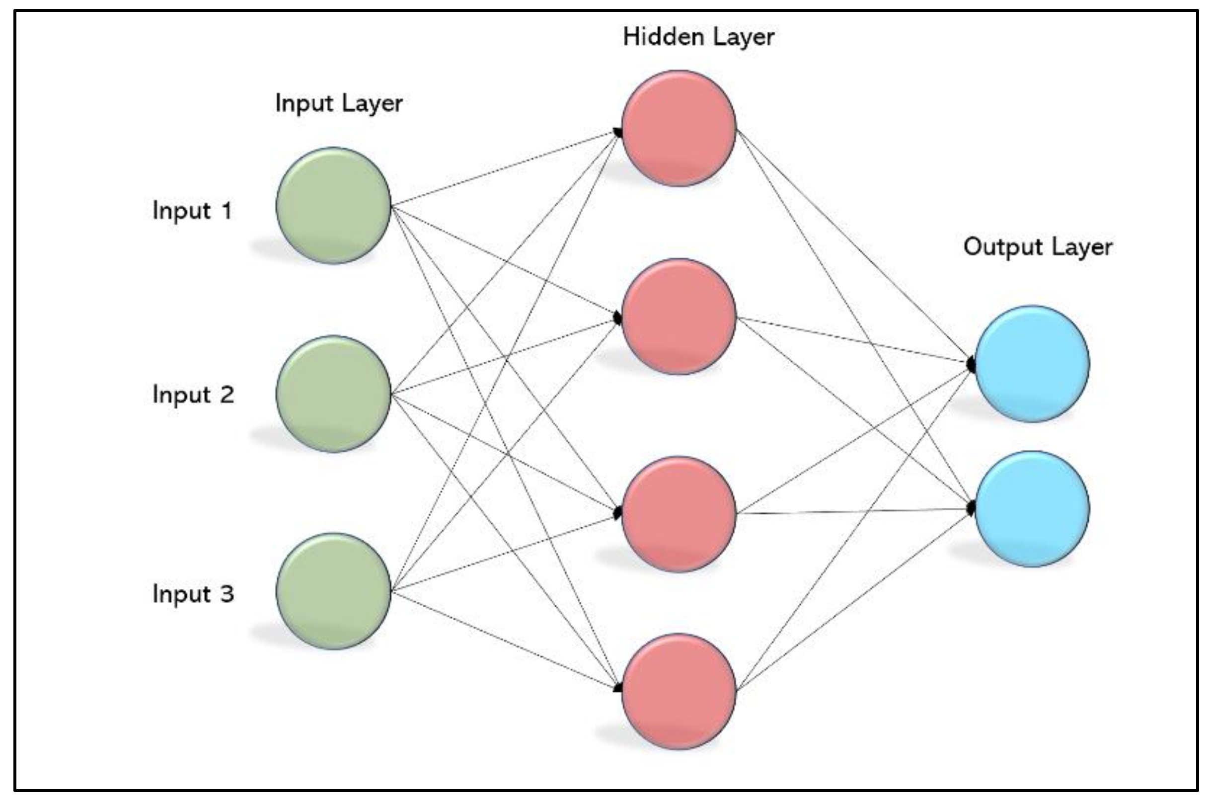
The first machine learning technique used in this work was the ANN, which is a computing system that is designed to mimic the way the biological systems, such as the human or animal brains, behave. ANN is developed to identify, estimate, classify, or make a decision by using a machine program. ANN is available in different structures; the simplest ANN structure, which was used in this study, is called multi-layered perceptron (MLP) which consists of one input layer, one or several hidden (learning) layers, and one output layer, as shown in Figure 1 [25]. The ANN systems are trained originally using training data (supervised learning) to perform the needed tasks [26].
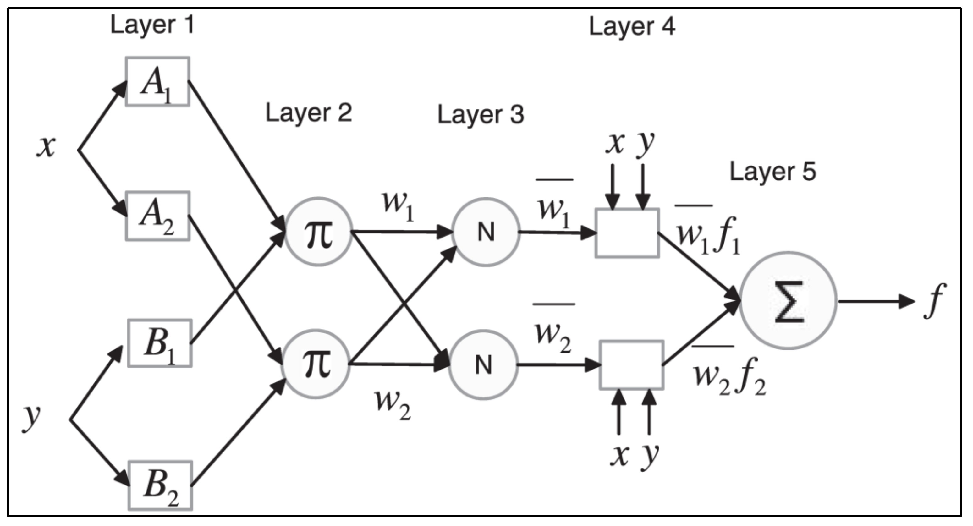
M-FIS was the second machine learning technique used in this study, which combines the adaptive neuro-fuzzy inference system (ANFIS) and subtractive clustering, where ANFIS is a multilayer feed-forward adaptive network in which the incoming signal will be subjected to a particular function performed by each training node where every node has its own parameters pertaining (Figure 2). The hybrid learning procedure was performed in two steps; the first step was the forward pass in which the functional signals representing the input data go forward and the least square formula was used to identify the parameters in the output layer (layer 5). The second step was the backward pass, in which the error rates propagate, in the opposite way, and the gradient method was implemented to update the parameters in the input layer (layer 1) [27].
The subtractive clustering is an unsupervised clustering algorithm that aims to examine the density of the available input data. Then it defines the point surrounded by the highest number of neighbors as the cluster’s center. It then subtracts (removes) the other data points within a pre-specified fuzzy radius, and the subtractive clustering algorithm considers only the point defined as the cluster’s center. This process is repeated to examine all input data points. Subtractive clustering generates the rules that approximate a function [28].
The third machine learning technique used in this study was the FNN model, compared to the ANN which uses the sigmoidal common model. The FNN model works with the generalized functional models. In FNN, the neuron’s function is learned from the existing data, which means they are not constant. Therefore, the weights related to links are not needed because the neuron functions include the effect of weights [29]. FNN contains an input layer, an output layer and layers of computing units that are related to each other. In FNN, there are different arguments in neural functions instead of one argument, such as in ANN [30].
The fourth machine learning model considered in this study was the SVM, which is one of the most famous classifying algorithms developed by Vapnik [31] in the framework of statistical learning theory. It performs classification of the data optimally into two or more divisions by applying a multidimensional hyperplane; this hyperplane is set to classify the data based on the tuning parameters (design parameters) of the kernel, regularization parameter (C), gamma, and margin. In its nature, SVM is very similar to a neural network, where the use of SVM with sigmoid kernel function is almost identical to the use of the perceptron neural network, having two hidden layers. Although it was originally developed in the statistical learning theory, the SVM technique is applicable in regression and classification problems, and it is also suitable for solving non-linear problems [32].
3. Applications of Machine Learning in Petroleum Engineering
Machine learning techniques are used in several scientific and engineering fields since the early 1990s to solve complicated non-linear problems. Petroleum engineers and petroleum geologists use different machine learning techniques to solve problems related to petroleum industry, such as the characterization of the heterogeneous hydrocarbon reservoirs [33,34], evaluation of the reserve of unconventional reservoirs [35,36,37,38], estimation of the rock mechanical parameters, such as the static Poisson’s ratio in carbonate reservoirs [39] and the static Young’s modulus for sandstone reservoirs [24,40], evaluation of the integrity of wellbore casing [41,42], optimization of drilling hydraulics [43], evaluation of pore pressure and fracture pressure [44,45], hydrocarbon recovery factor estimation [46,47], determination of the alteration in the drilling fluids rheology in real-time [48,49], optimization of rate of penetration [50,51], prediction of the formation tops [52], and others.
4. Application to the Well Log Data
The predictability of the machine learning models depends on the amount of training data points and the design parameters of every model. In this work, the machine learning model’s design parameters and the selection of the optimum training data points were conducted based on the optimization process of all combinations of the design parameters, as will be discussed in the following sections.
4.1. Data Preparation
The machine learning models are trained in this study to predict Estatic based on the RHOB, DTs, and DTc as inputs. In this study, core-derived Estatic and their corresponding well log data collected from two different sandstone wells (598 collected from Well-A and 38 from Well-B) were used. The data of Well-A was used to build and test the machine learning models, and Well-B data (unseen data) was used to validate the trained machine learning models. Both formations considered in wells A and B were sandstone formations.
Before training the machine learning models, the data were studied statistically to remove all noise, unreal values, and outliers from the training data. The standard deviation (SD) was considered for removing the outliers; based on this, all data points without the range of ± 3.0 SD were considered as outliers and removed from the input dataset. This preprocessing is very important to ensure accurate estimation of the targeted parameter by applying the machine learning techniques [53]. Out of the 598 data points collected from Well-A, 6 data points were considered as outliers, these data points were removed from the data before the start of the training process.
Since the core derived Estatic was estimated based on well log data, it was very important to perform depth matching between the well log input data and core derived Estatic. Although the gamma-ray log was not considered as input in this study, it was considered at this step to perform the depth matching.
4.2. Training the Machine Learning Models
After data preprocessing, 592 well log data points and their corresponding core derived Estatic were considered valid for machine learning models training. Four hundred and fourteen, 178, 355, and 444 well log data points (out of the 592) were considered to train ANN, M-FIS, FNN, and SVM models, respectively. The number of the training data was selected based on the optimization process, where the optimum number of the training data that optimize the predictability of the different machine learning models was selected in every case. The statistical characteristics for the training datasets for the different machine learning models are summarized in Table 1. The data of Table 1 is very important when the machine learning models are to be used for evaluating Estatic for a new dataset; the new testing data should be within the ranges in Table 1.
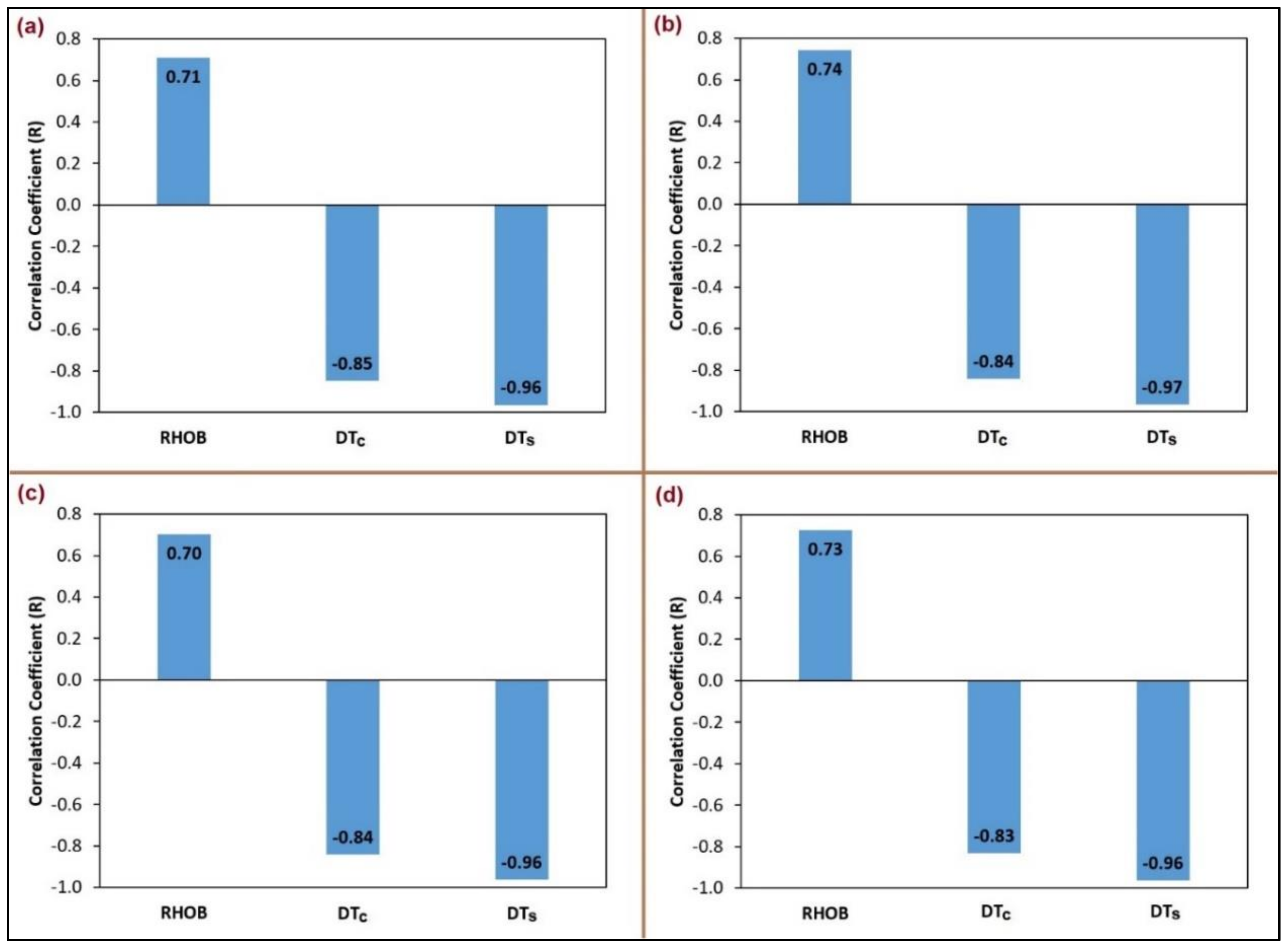
The input training well logs data were selected based on their relative importance on the actual Estatic which was determined in this study based on the correlation coefficient (R), Figure 3 compares R for the input well log data used to train the different machine learning model. As indicated in Figure 3, all well log parameters used to train the machine learning models are strongly related to Estatic with high Rs of >0.7 for the bulk density, >0.8 for the compressional transit time, and >0.95 for the shear transit time.
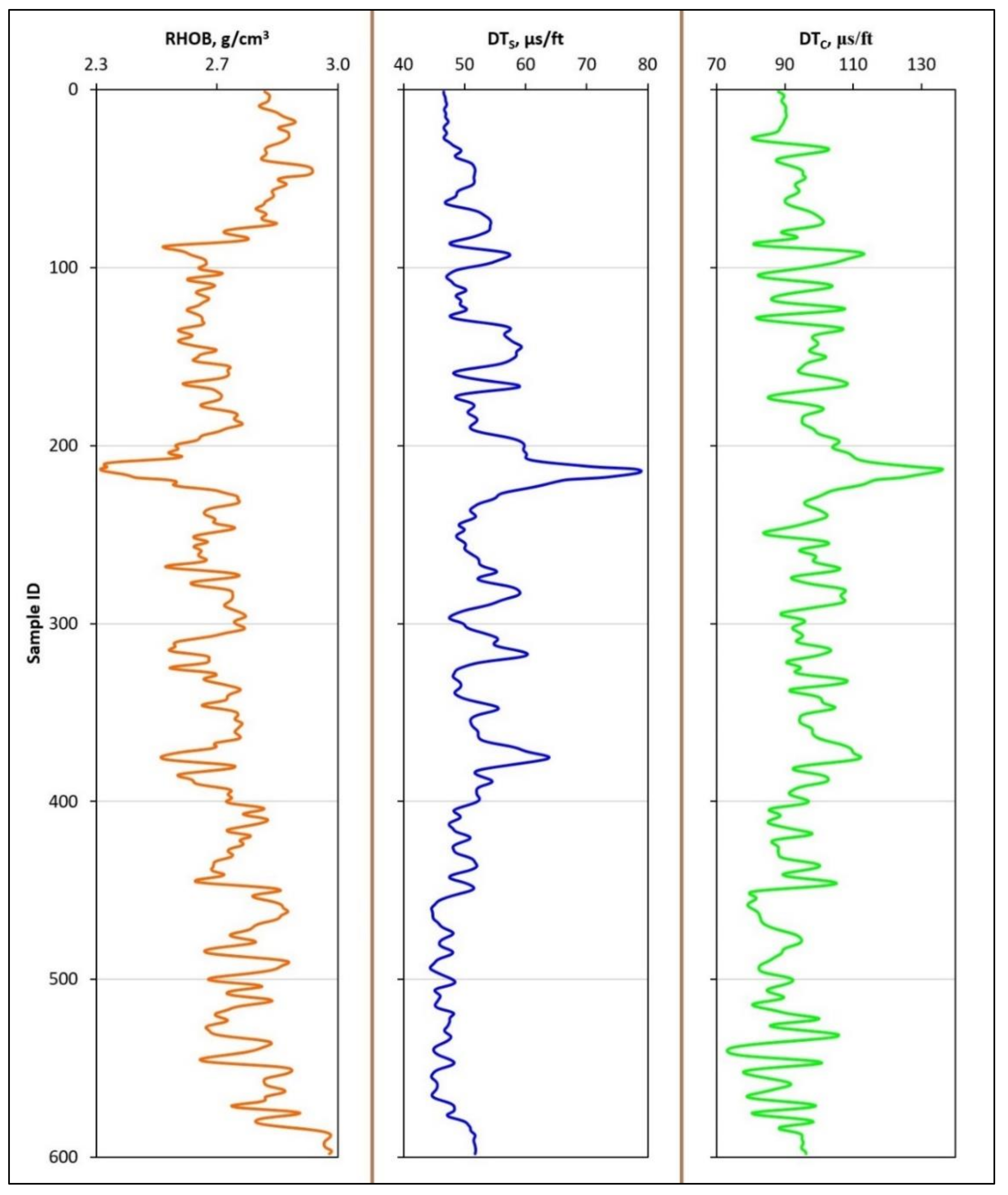
Figure 4 shows the inputs used to learn the machine learning models. Inserted for loops were designed using MATLAB software to optimize all combinations of the machine learning model’s design parameters for Estatic estimation; every single for loop represents one design parameter. Sensitivity analysis was conducted to evaluate the effect of changing every single design parameter on the predictability of Estatic by the different machine learning models considered in this study. The sensitivity analysis is a critical step in optimizing the design parameters of the machine learning models and several previous studies considered it as a crucial step in optimizing the performance of different mathematical models [54,55,56]. Based on the sensitivity analysis results, the combinations of the variables in Table 2 were found to optimize Estatic estimation using the different machine learning models; these parameters predicted Estatic with the lowest average absolute percentage error (AAPE) and the highest R; the AAPE was calculated using Equation (3).
where N represents the number of the data points, a and m denote the actual and estimated Estatic, respectively.
4.3. Evaluation of the Developed Machine Learning Models
After training, the developed machine learning models were then tested using the remaining data collected from the same training sandstone formation in Well-A and then validated using 38 data points (unseen data) collected from a sandstone formation in Well-B.
Uncertainty quantification is at the heart of decision making, especially in subsurface applications. Uncertainty about the geological structures, rocks, and fluids is because of the lack of access to the subsurface geological medium [57,58]. The uncertainty in the prediction results of all machine learning models developed in this study was directly controlled by the uncertainty on the well log data used to develop these models which were highly controlled by the depth of investigation and vertical resolution of every logging tool.
5. Results and Discussion
5.1. Machine Learning Models Development
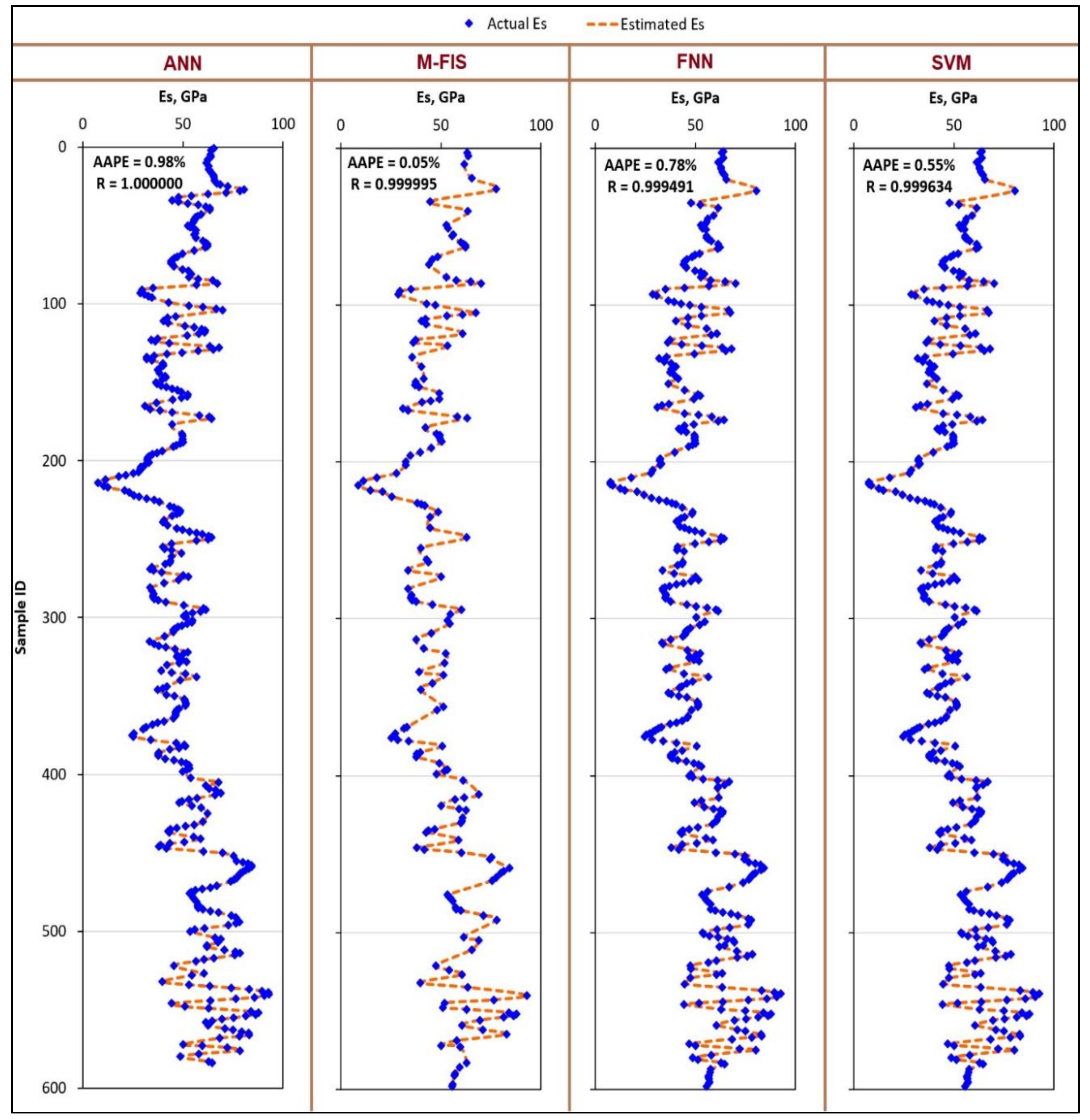
The machine learning models were trained to predict Estatic as a function of the RHOB, DTs, and DTc. The training data were collected from Well-A. Figure 5 compares the actual and estimated Estatic for the training dataset.
Figure 5 shows that all machine learning models predicted Estatic with very high accuracy. M-FIS predicted Estatic with AAPE of only 0.05% and R of 0.999995. FNN model estimated the Estatic with AAPE and R of 0.78% and 0.999491, respectively, while SVM model estimated Estatic with AAPE of 0.55% and R of 0.999634, and the ANN model predicted Estatic with AAPE of 0.98% and R of 1.000000. The good matching between the actual and estimated Estatic for the training dataset shown in Figure 5 proves the high accuracy of the machine learning models in evaluating Estatic.
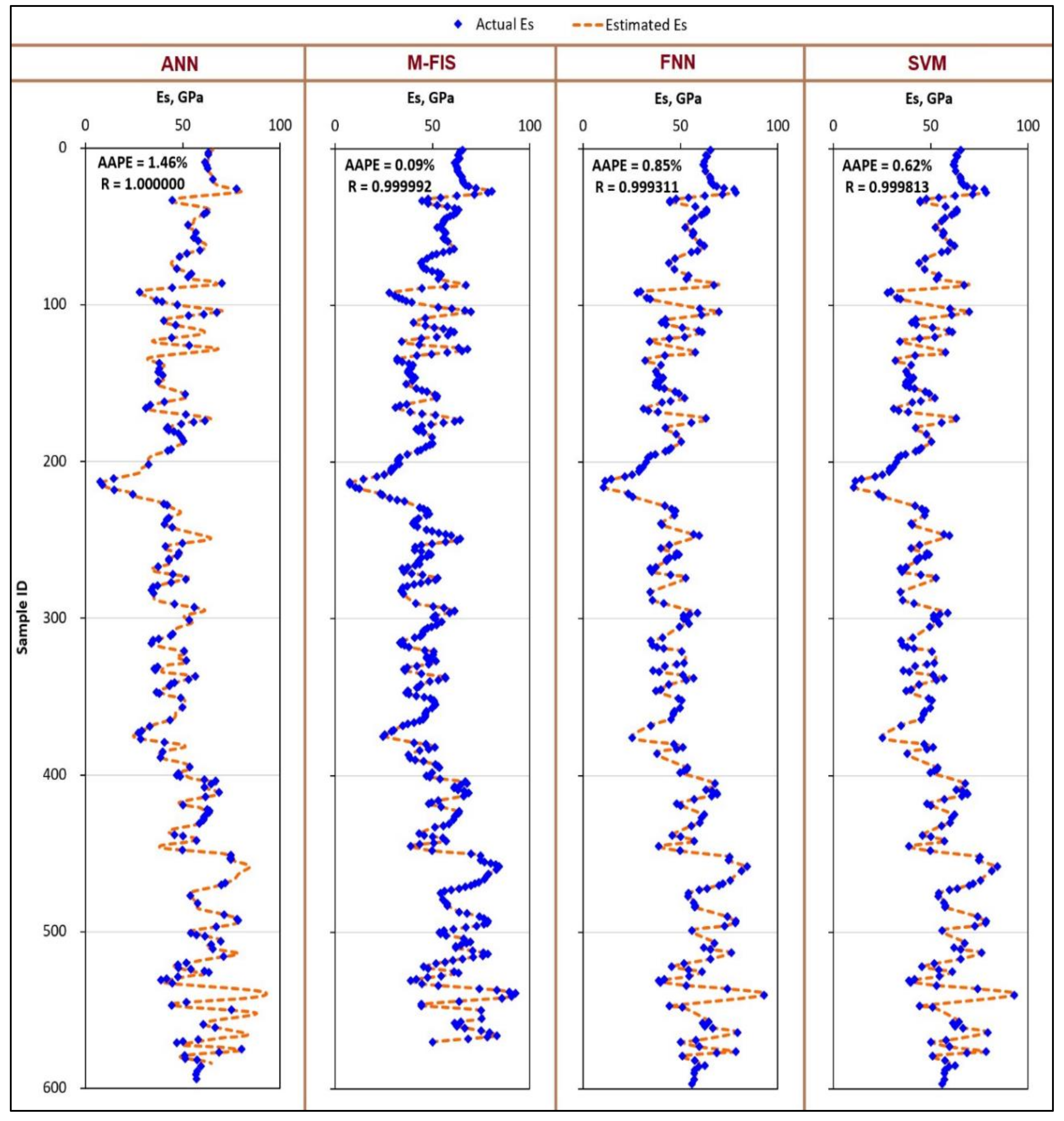
5.2. Testing the Developed Machine Learning Models
The performance of the developed machine learning models in evaluating the Estatic for the testing dataset, which was collected from the same training formation used to developed machine learning models (i.e., from Well-A), was evaluated. As indicated in Figure 6, all machine learning models predicted Estatic with very high accuracy. M-FIS predicted Estatic for the testing dataset with AAPE and R of 0.09% and 0.999992, respectively, FNN model predicted Estatic with AAPE of 0.85% and R of 0.999311, then SVM model which estimated Estatic with an AAPE and R of 0.62% and 0.999813, respectively, and the ANN estimated Estatic with AAPE of 1.46% and R of 1.000000. Visual check of the actual and estimated Estatic of the testing data set also confirmed the high accuracy of the machine learning models, as indicated by the good matching between the actual and estimated Estatic.
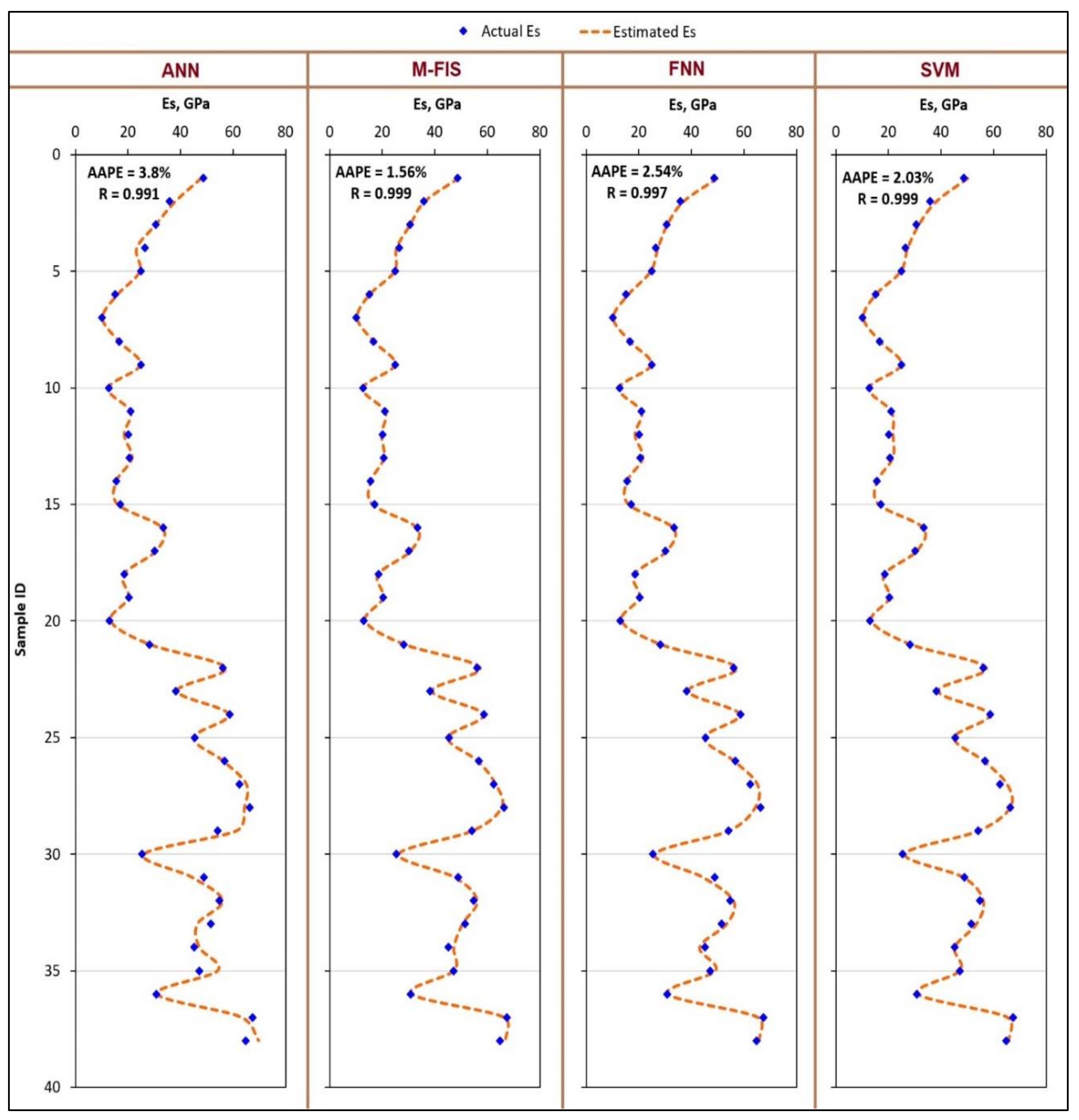
5.3. Validation of the Developed Machine Learning Models
The machine learning models’ accuracy was finally validated using 38 data points collected from another sandstone formation in Well-B. Figure 7 compares the actual core derived and estimated Estatic using the developed machine learning for the validation data set. The results in Figure 7 confirmed that all machine learning models predicted Estatic with very high accuracy. This figure also confirmed that M-FIS technique is the best among the others on estimating Estatic for the validation data set, where the developed M-FIS predicted Estatic with AAPE of 1.56% and R of 0.999, followed by SVM model which predicted Estatic with AAPE of 2.03% and R of 0.999, then FNN model which estimated Estatic with AAPE of 2.54% and R of 0.997, and the least accurate model was the ANN which predicted Estatic with AAPE of 3.80% and R of 0.991.
A visual check of the actual and estimated Estatic of the validation data set also confirmed the high accuracy of all machine learning models considered in this work, as confirmed by the good matching between the estimated and core derived Estatic. A continuous profile of Estatic along the drilled sections of Well-B was obtained using the machine learning models. This is not possible to achieve by conducting laboratory work only. The confidence intervals for the validation data were ± 0.574, ± 0.804, ± 0.843, and ± 0.877, with a confidence level of 99% for M-FIS, SVM, ANN, and FNN models, respectively.
Figure 8 compares the AAPE for the calculated Estatic for training, testing, and validation datasets using the different machine learning models. This figure confirms that the developed M-FIS model overperformed the other machine learning models in predicting Estatic for the training, testing, and validation datasets in terms of AAPE. M-FIS predicted Estatic with the lowest AAPE of 1.56 %, while the AAPE for the SVM, FNN, and ANN were 2.03, 2.54, and 3.80, respectively.
Out of the results of training, testing, and validation data and considering the similarity of the results of the evaluation parameters (AAPE and R) and taking into consideration that adding or omitting a few points may change the highest-to-lowest order of the models accuracy, we conclude that the four models are equally adequate to estimate Estatic using only the conventional well log used in this study. Nevertheless, we recommend using the M-FIS model as it is the best-performed model for estimating Estatic for the training, testing, and validation data.
The machine learning models developed in this work are very helpful for the petroleum engineers and petroleum industry since they could positively improve Estatic estimation, therefore, enabling petroleum engineers and geoscientists to construct the earth geomechanical map and to evaluate the wellbore stability condition, the reservoir compaction, hydraulic fracturing, and the formation control [1,3].
6. Conclusions
Four machine learning techniques were applied in this study to develop models for estimating Estatic for sandstone formations, these machine learning techniques were ANN, FNN, M-FIS, and SVM. The machine learning models were trained to evaluate Estatic based on conventional well log data of the RHOB, DTs, and DTc. The machine learning models were trained and tested based on data gathered from sandstone formation in Well-A and then the developed models were validated on unseen data collected from a sandstone formation in Well-B. The outcomes of this work confirmed the high accuracy of all machine learning models, and M-FIS models overperformed all others in estimating Estatic for training, testing, and validation data sets. For the validation data, M-FIS predicted Estatic with a very low AAPE of 1.56% and R of 0.999. The high accuracy of the developed machine learning models was also confirmed by visual comparison of the estimated and actual Estatic.
Author Contributions
Conceptualization, S.E; data preparation, S.E., and A.A.M.; models development, A.A.M.; results analysis, A.A.M.; writing—original draft preparation, A.A.M.; writing—review and editing, S.E., and D.A.S.; supervision, S.E. All authors have read and agreed to the published version of the manuscript.
Conflicts of Interest
The authors declare no conflict of interest.
Nomenclature
| AAPE | Average absolute percentage error |
| ANN | Artificial neural networks |
| DTc | Compressional transit time |
| DTs | Shear transit time |
| Edynamic | Dynamic Young’s modulus |
| Estatic | Static Young’s modulus |
| FNN | Functional neural networks |
| M-FIS | Mamdani fuzzy interference system |
| SVM | Support vector machine |
| R | Correlation coefficient |
| RHOB | Formation bulk density |
References
- Britt, L.K.; Smith, M.B.; Haddad, Z.; Reese, J.; Kelly, P. Rotary Sidewall Cores—A Cost Effective Means of Determining Young’s Modulus. Proceeding of the SPE Annual Technical Conference and Exhibition, Houston, TX, USA, 26–29 September 2004. [Google Scholar] [CrossRef]
- Fjaer, E.; Horsrud, H.P.; Raaen, A.M.; Risnes, R. Petroleum Related Rock Mechanics, 2nd ed.; Elsevier Science: Amsterdam, The Netherlands, 2008; Volume 53, ISBN 9780080557090. [Google Scholar]
- Chang, C.; Zoback, M.D.; Khaksar, A. Empirical relations between rock strength and physical properties in sedimentary rocks. J. Pet. Sci. Eng. 2006, 51, 223–237. [Google Scholar] [CrossRef]
- Gatens, J.M.; Harrison, C.W.; Lancaster, D.E.; Guldry, F.K. In-situ stress tests and acoustic logs determine mechanical properties and stress profiles in the Devonian shales. SPE Form. Eval. 1990, 5, 248–254. [Google Scholar] [CrossRef]
- Meyer, B.R.; Jacot, R.H. Impact of Stress-Dependent Young’s Moduli on Hydraulic Fracture Modeling. In Proceedings of the 38th U.S. Symposium on Rock Mechanics, Washington, DC, USA, 7–10 July 2001. [Google Scholar]
- Nes, O.M.; Fjaer, E.; Tronvoll, J.; Kristiansen, T.G.; Horsrud, P. Drilling time reduction through an integrated rock mechanics analysis. J. Energy Resour. Technol. 2012, 134, 032802. [Google Scholar] [CrossRef]
- Howard, G.C.; Fast, C.R. Hydraulic Fracturing. In Doherty Memorial Fund of AIME, Society of Petroleum Engineers of AIME; Henry L.: New York, NY, USA, 1970; Volume 2, ISBN 10. [Google Scholar]
- Barree, R.D.; Gilbert, J.V.; Conway, M.W. Stress and Rock Property Profiling for Unconventional Reservoir Stimulation. In Proceedings of the SPE Hydraulic Fracturing Technology Conference, The Woodlands, TX, USA, 19–21 January 2009. [Google Scholar] [CrossRef]
- Rinehart, J.S.; Fortin, J.-P.; Burgin, L. Propagation Velocity of Longitudinal Waves in Rock. Effect of State of Stress, Stress Level of the Wave, Water Content, Porosity, Temperature Stratification and Texture. In Proceedings of the 4th Symposium on Rock Mechanics, University Park, PA, USA, 30 March–1 April 1961. [Google Scholar]
- Simmons, G.; Brace, W.F. Comparison of Static and Dynamic Measurements of Compressibility of Rocks. J. Geophys. Res. 1965, 70, 5649–5656. [Google Scholar] [CrossRef]
- King, M.S. Wave Velocities in Rocks as a Function of Changes in over burden Pressure and Pore Fluid Saturants. Geophysics 1966, 31, 50–73. [Google Scholar] [CrossRef]
- Larsen, I.; Fjær, E.; Renlie, L. Static and Dynamic Poisson’s Ratio of Weak Sandstones. In Proceedings of the 4th North American Rock Mechanics Symposium, Seattle, WA, USA, 31 July–3 August 2000. [Google Scholar]
- Hui, C.; Lian-Ku, X.; Li-Jie, G.; Hu-Xin, W.; Biao, C. Rock mechanics study on the safety and efficient extraction for deep moderately inclined medium-thick orebody. Electron. J. Geotech. Eng. 2015, 20, 11073–11082. [Google Scholar]
- Peng, L.; Xinrong, L.; Zuliang, Z. Mechanical Property Experiment and Damage Statistical Constitutive Model of Hongze Rock Salt in China. Electron. J. Geotech. Eng. 2015, 20, 81–94. [Google Scholar]
- King, M.S. Static and Dynamic elastic moduli of rocks under pressure. In Proceedings of the 11th U.S. Symposium on Rock Mechanics (USRMS), Berkeley, CA, USA, 16–19 June 1969. [Google Scholar]
- Canady, W.J. A Method for Full-Range Young’s Modulus Correction. In Proceedings of the North American Unconventional Gas Conference and Exhibition, The Woodlands, TX, USA, 14–16 June 2011. [Google Scholar] [CrossRef]
- Khaksar, A.; Taylor, P.G.; Fang, Z.; Kayes, T.J.; Salazar, A.; Rahman, K. Rock Strength from Core and Logs, Where We Stand and Ways to Go. In Proceedings of the EUROPEC/EAGE Conference and Exhibition, Amsterdam, The Netherlands, 8–11 June 2009. [Google Scholar] [CrossRef]
- Fei, W.; Huiyuan, B.; Jun, Y.; Yonghao, Z. Correlation of Dynamic and Static Elastic Parameters of Rock. Electronic J. Geotech. Eng. 2016, 21, 1551–1560. [Google Scholar]
- Mahmoud, M.A.; Elkatatny, S.A.; Ramadan, E.; Abdulraheem, A. Development of Lithology-Based Static Young’s Modulus Correlations from Log Data Based on Data Clustering Technique. J. Pet. Sci. Eng. 2016, 146, 10–20. [Google Scholar] [CrossRef]
- Abdulraheem, A.; Ahmed, M.; Vantala, A.; Parvez, T. Prediction of Rock Mechanical Parameters for Hydrocarbon Reservoirs Using Different Artificial Intelligence Techniques. In Proceedings of the SPE Saudi Arabia Section Technical Symposium, Al-Khobar, Saudi Arabia, 9–11 May 2009. [Google Scholar] [CrossRef]
- Tariq, Z.; Elkatatny, S.; Mahmoud, M.; Abdulraheem, A. A New Artificial Intelligence Based Empirical Correlation to Predict Sonic Travel Time. In Proceedings of the International Petroleum Technology Conference, Bangkok, Thailand, 14–16 November 2016. [Google Scholar] [CrossRef]
- Tariq, Z.; Elkatatny, S.M.; Mahmoud, M.A.; Abdulraheem, A.; Abdelwahab, A.Z.; Woldeamanuel, M. Estimation of Rock Mechanical Parameters Using Artificial Intelligence Tools. In Proceedings of the 51st U.S. Rock Mechanics/Geomechanics Symposium, San Francisco, CA, USA, 25–28 June 2017. [Google Scholar]
- Parapuram, G.K.; Mokhtari, M.; Hmida, J.B. Prediction and Analysis of Geomechanical Properties of the Upper Bakken Shale Utilizing Artificial Intelligence and Data Mining. In Proceedings of the SPE/AAPG/SEG Unconventional Resources Technology Conference, Austin, TX, USA, 24–26 July 2017. [Google Scholar] [CrossRef]
- Mahmoud, A.A.; Elkatatny, S.; Ali, A.; Moussa, T. Estimation of Static Young’s Modulus for Sandstone Formation Using Artificial Neural Networks. Energies 2019, 12, 2125. [Google Scholar] [CrossRef] [Green Version]
- Mahmoud, A.A.A.; Elkatatny, S.; Mahmoud, M.; Abouelresh, M.; Abdulraheem, A.; Ali, A. Determination of the total organic carbon (TOC) based on conventional well logs using artificial neural network. Int. J. Coal Geol. 2017, 179, 72–80. [Google Scholar] [CrossRef]
- Gurney, K. An Introduction to Neural Networks; UCL Press Limited: London, UK, 1997; ISBN 0-203-45151-1. [Google Scholar]
- Jang, R. ANFIS Adaptive Network Based Fuzzy Inference System. IEEE Trans. Syst. Man Cybern. 1993, 23, 665–685. [Google Scholar] [CrossRef]
- Jang, J.S.R.; Sun, C.T.; Mizutani, E. Neuro-Fuzzy and Soft Computing; Prentice Hall: Bergen, NJ, USA, 1997; ISBN 0132610663. [Google Scholar]
- Bello, O.; Asafa, T. A Functional Networks Softsensor for Flowing Bottomhole Pressures and Temperatures in Multiphase Production Wells. In Proceeding of the SPE Intelligent Energy Conference & Exhibition, Utrecht, The Netherlands, 1–3 April 2014. [Google Scholar] [CrossRef]
- Anifowose, F.; Abdulraheem, A. Fuzzy logic-driven and SVM-driven hybrid computational intelligence models applied to oil and gas reservoir characterization. J. Natl. Gas Sci. Eng. 2011, 3, 505–517. [Google Scholar] [CrossRef]
- Vapnik, V. Statistical Learning Theory; Wiley: New York, NY, USA, 1998; ISBN 978-0471030034. [Google Scholar]
- Rui, J.; Zhang, H.; Zhang, D.; Han, F.; Guo, Q. Total organic carbon content prediction based on support-vector-regression machine with particle swarm optimization. J. Pet. Sci. Eng. 2019, 180, 699–706. [Google Scholar] [CrossRef]
- Mohaghegh, S.; Arefi, R.; Ameri, S.; Hefner, M.H. A Methodological Approach for Reservoir Heterogeneity Characterization Using Artificial Neural Networks. In Proceedings of the SPE Annual Technical Conference and Exhibition, New Orleans, LA, USA, 25–28 September 1994. [Google Scholar] [CrossRef]
- Barman, I.; Ouenes, A.; Wang, M. Fractured Reservoir Characterization Using Streamline-Based Inverse Modeling and Artificial Intelligence Tools. In Proceedings of the SPE Annual Technical Conference and Exhibition, Dallas, TX, USA, 1–4 October 2000. [Google Scholar] [CrossRef]
- Mahmoud, A.A.; Elkatatny, S.; Abdulraheem, A.; Mahmoud, M.; Ibrahim, M.O.; Ali, A. New Technique to Determine the Total Organic Carbon Based on Well Logs Using Artificial Neural Network (White Box). In Proceedings of the SPE Kingdom Saudi Arabia Annual Technical Symposium and Exhibition, Dammam, Saudi Arabia, 24–27 April 2017. [Google Scholar] [CrossRef]
- Mahmoud, A.A.; Elkatatny, S.; Ali, A.; Abouelresh, M.; Abdulraheem, A. Evaluation of the Total Organic Carbon (TOC) Using Different Artificial Intelligence Techniques. Sustainability 2019, 11, 5643. [Google Scholar] [CrossRef] [Green Version]
- Mahmoud, A.A.; Elkatatny, S.; Ali, A.; Abouelresh, M.; Abdulraheem, A. New Robust Model to Evaluate the Total Organic Carbon Using Fuzzy Logic. In Proceedings of the SPE Kuwait Oil & Gas Show and Conference, Mishref, Kuwait, 13–16 October 2019. [Google Scholar] [CrossRef]
- Mahmoud, A.A.; Elkatatny, S.; Abouelresh, M.; Abdulraheem, A.; Ali, A. Estimation of the Total Organic Carbon Using Functional Neural Networks and Support Vector Machine. In Proceedings of the 12th International Petroleum Technology Conference and Exhibition, Dhahran, Saudi Arabia, 13–15 January 2020. [Google Scholar] [CrossRef]
- Elkatatny, S. Application of Artificial Intelligence Techniques to Estimate the Static Poisson’s Ratio Based on Wireline Log Data. J. Energy Resour. Technol. 2018, 140, 072905. [Google Scholar] [CrossRef]
- Mahmoud, A.A.; Elkatatny, S.; Ali, A.; Moussa, T. A Self-adaptive Artificial Neural Network Technique to Estimate Static Young’s Modulus Based on Well Logs. Proceedings of Oman Petroleum & Energy Show, Muscat, Oman, 9–11 March 2020. [Google Scholar] [CrossRef]
- Al-Shehri, D.A. Oil and Gas Wells: Enhanced Wellbore Casing Integrity Management through Corrosion Rate Prediction Using an Augmented Intelligent Approach. Sustainability 2019, 11, 818. [Google Scholar] [CrossRef] [Green Version]
- Salehi, S.; Hareland, G.; Dehkordi, K.K.; Ganji, M.; Abdollahi, M. Casing collapse risk assessment and depth prediction with a neural network system approach. J. Petrol. Sci. Eng. 2009, 69, 156–162. [Google Scholar] [CrossRef]
- Wang, Y.; Salehi, S. Application of real-time field data to optimize drilling hydraulics using neural network approach. J. Energy Resour. Technol. 2015, 137, 062903. [Google Scholar] [CrossRef]
- Ahmed, A.S.; Mahmoud, A.A.; Elkatatny, S. Fracture Pressure Prediction Using Radial Basis Function. In Proceedings of the AADE National Technical Conference and Exhibition, Denver, CO, USA, 9–10 April 2019. [Google Scholar]
- Ahmed, A.S.; Mahmoud, A.A.; Elkatatny, S.; Mahmoud, M.; Abdulraheem, A. Prediction of Pore and Fracture Pressures Using Support Vector Machine. In Proceedings of the 2019 International Petroleum Technology Conference, Beijing, China, 26–28 March 2019. [Google Scholar] [CrossRef]
- Mahmoud, A.A.; Elkatatny, S.; Abdulraheem, A.; Mahmoud, M. Application of Artificial Intelligence Techniques in Estimating Oil Recovery Factor for Water Drive Sandy Reservoirs. In Proceedings of the SPE Kuwait Oil & Gas Show and Conference, Kuwait City, Kuwait, 15–18 October 2017. [Google Scholar] [CrossRef]
- Mahmoud, A.A.; Elkatatny, S.; Chen, W.; Abdulraheem, A. Estimation of Oil Recovery Factor for Water Drive Sandy Reservoirs through Applications of Artificial Intelligence. Energies 2019, 12, 3671. [Google Scholar] [CrossRef] [Green Version]
- Abdelgawad, K.Z.; Elzenary, M.; Elkatatny, S.; Mahmoud, M.; Abdulraheem, M.; Patil, S. New approach to evaluate the equivalent circulating density (ECD) using artificial intelligence techniques. J. Petrol. Explor. Prod. Technol. 2019, 9, 1569. [Google Scholar] [CrossRef] [Green Version]
- Elkatatny, S.M. Real Time Prediction of Rheological Parameters of KCl Water-Based Drilling Fluid Using Artificial Neural Networks. Arab. J. Sci. Eng. 2017, 42, 1655–1665. [Google Scholar] [CrossRef]
- Al-AbdulJabbar, A.; Elkatatny, S.; Mahmoud, A.A.; Moussa, T.; Al-Shehri, D.; Abughaban, M.; Al-Yami, A. Prediction of the Rate of Penetration while Drilling Horizontal Carbonate Reservoirs Using the Self-Adaptive Artificial Neural Networks Technique. Sustainability 2020, 12, 1376. [Google Scholar] [CrossRef] [Green Version]
- Al-AbdulJabbar, A.; Elkatatny, S.M.; Mahmoud, M.; Abdelgawad, K.; Abdulaziz, A. A Robust Rate of Penetration Model for Carbonate Formation. J. Energy Resour. Technol. 2018, 141, 042903. [Google Scholar] [CrossRef]
- Elkatatny, S.; Al-AbdulJabbar, A.; Mahmoud, A.A. New Robust Model to Estimate the Formation Tops in Real-Time Using Artificial Neural Networks (ANN). Petrophysics 2019, 60, 825–837. [Google Scholar] [CrossRef]
- Al-Anazi, A.F.; Gates, I.D. A support vector machine algorithm to classify lithofacies and model permeability in heterogeneous reservoirs. Eng. Geol. 2010, 114, 267–277. [Google Scholar] [CrossRef]
- Daniel, C. One-at-a-Time plans. J. Am. Stat. Assoc. 1973, 68, 353–360. [Google Scholar] [CrossRef]
- Sobol’, I.M. Global sensitivity indices for nonlinear mathematical models and their Monte Carlo estimates. Math. Comput. Simul. 2001, 55, 271–280. [Google Scholar] [CrossRef]
- Yin, Z.; Feng, T.; MacBeth, C. Fast assimilation of frequently acquired 4D seismic data for reservoir history matching. Comput. Geosci. 2019, 128, 30–40. [Google Scholar] [CrossRef]
- Hermans, T.; Nguyen, F.; Klepikova, M.; Dassargues, A.; Caers, J. Uncertainty Quantification of Medium-Term Heat Storage from Short-Term Geophysical Experiments Using Bayesian Evidential Learning. Water Resour. Res. 2018, 54, 2931–2948. [Google Scholar] [CrossRef] [Green Version]
- Yin, Z.; Strebelle, S.; Caers, J. Automated Monte Carlo-based Quantification and Updating of Geological Uncertainty with Borehole Data (AutoBEL v1.0). Geosci. Model. Dev. 2019, 13. [Google Scholar] [CrossRef] [Green Version]
Figure 1.
Artificial neural networks model with input layers of three inputs, one hidden layer, and an output layer.
Figure 1.
Artificial neural networks model with input layers of three inputs, one hidden layer, and an output layer.

Figure 2.
Adaptive neuro-fuzzy inference system architecture of a model using two inputs layers and one output parameter.
Figure 2.
Adaptive neuro-fuzzy inference system architecture of a model using two inputs layers and one output parameter.

Figure 3.
Comparison of the relative importance of the training parameters used to develop (a) ANN, (b) the Mamdani fuzzy interference system (M-FIS), (c) functional neural networks (FNN), and (d) support vector machine (SVM) models.
Figure 3.
Comparison of the relative importance of the training parameters used to develop (a) ANN, (b) the Mamdani fuzzy interference system (M-FIS), (c) functional neural networks (FNN), and (d) support vector machine (SVM) models.

Figure 4.
The training input well log data collected from Well-A.

Figure 5.
Actual and estimated static Young’s modulus (Estatic) for the training dataset collected from Well-A.
Figure 5.
Actual and estimated static Young’s modulus (Estatic) for the training dataset collected from Well-A.

Figure 6.
Actual and estimated Estatic for the testing dataset collected from Well-A.

Figure 7.
Core-derived and predicted Estatic for the validation dataset collected from Well-B.

Figure 8.
Comparison of the AAPE for the training, testing, and validation datasets for all machine learning models.
Figure 8.
Comparison of the AAPE for the training, testing, and validation datasets for all machine learning models.


Table 1.
The statistical characteristics for the training data set.
| Artificial Neural Networks. | ||||
|---|---|---|---|---|
| RHOB, g/cm3 | DTc, μs/ft | DTs, μs/ft | Estatic, GPa | |
| Minimum | 2.32 | 44.4 | 73.2 | 7.50 |
| Maximum | 2.98 | 78.9 | 136 | 92.8 |
| Range | 0.66 | 34.6 | 62.4 | 85.3 |
| Standard Deviation | 0.114 | 5.06 | 8.91 | 14.9 |
| Sample Variance | 0.013 | 25.6 | 79.4 | 221 |
| Mamdani Fuzzy Interference System | ||||
| RHOB, g/cm3 | DTc, μs/ft | DTs, μs/ft | Estatic, GPa | |
| Minimum | 2.33 | 44.6 | 73.2 | 8.63 |
| Maximum | 2.98 | 78.7 | 133 | 92.8 |
| Range | 0.66 | 34.1 | 60.0 | 84.2 |
| Standard Deviation | 0.114 | 5.45 | 9.47 | 15.2 |
| Sample Variance | 0.013 | 29.7 | 89.6 | 232 |
| Functional Neural Networks | ||||
| RHOB, g/cm3 | DTc, μs/ft | DTs, μs/ft | Estatic, GPa | |
| Minimum | 2.31 | 44.5 | 73.6 | 7.50 |
| Maximum | 2.98 | 78.9 | 136 | 92.6 |
| Range | 0.67 | 34.4 | 62.5 | 85.1 |
| Standard Deviation | 0.112 | 5.27 | 9.20 | 14.9 |
| Sample Variance | 0.013 | 27.7 | 84.7 | 222 |
| Support Vector Machine | ||||
| RHOB, g/cm3 | DTc, μs/ft | DTs, μs/ft | Estatic, GPa | |
| Minimum | 2.31 | 44.3 | 73.2 | 7.50 |
| Maximum | 2.98 | 78.9 | 136 | 92.8 |
| Range | 0.67 | 34.6 | 62.9 | 85.3 |
| Standard Deviation | 0.113 | 5.21 | 8.99 | 14.5 |
| Sample Variance | 0.013 | 27.1 | 80.8 | 210 |
Table 2.
Optimized design parameters for the machine learning models.
| Artificial Neural Networks | |
|---|---|
| Training Data (out of total data from Well-A) | 70% |
| Testing Data (out of total data from Well-A) | 30% |
| Learning Function | Trainbr |
| Transfer Function | Logsig |
| Number of Training Layers | Single Layer |
| Neurons per Training Layer | 20 |
| Mamdani Fuzzy Interference System | |
| Training Data (out of total data from Well-A) | 30% |
| Testing Data (out of total data from Well-A) | 70% |
| Cluster Radius | 0.3 |
| Number of Iterations | 180 |
| Functional Neural Networks | |
| Training Data (out of total data from Well-A) | 60% |
| Testing Data (out of total data from Well-A) | 40% |
| Training Method | Forward Selection Method |
| Function Type | Non-linear Function with No Iteration Terms |
| Support Vector Machine | |
| Training Data (out of total data from Well-A) | 75% |
| Testing Data (out of total data from Well-A) | 25% |
| Verbose | 0.7 |
| C | 3000 |
| Epsilon | 0.5 |
| Lambda | 1 × 10⁻⁷ |
| Kernel | gaussian |
| Kerneloption | 9 |
© 2020 by the authors. Licensee MDPI, Basel, Switzerland. This article is an open access article distributed under the terms and conditions of the Creative Commons Attribution (CC BY) license (http://creativecommons.org/licenses/by/4.0/).
Share and Cite
MDPI and ACS Style
Mahmoud, A.A.; Elkatatny, S.; Al Shehri, D. Application of Machine Learning in Evaluation of the Static Young’s Modulus for Sandstone Formations. Sustainability 2020, 12, 1880. https://0-doi-org.brum.beds.ac.uk/10.3390/su12051880
AMA Style
Mahmoud AA, Elkatatny S, Al Shehri D. Application of Machine Learning in Evaluation of the Static Young’s Modulus for Sandstone Formations. Sustainability. 2020; 12(5):1880. https://0-doi-org.brum.beds.ac.uk/10.3390/su12051880
Chicago/Turabian StyleMahmoud, Ahmed Abdulhamid, Salaheldin Elkatatny, and Dhafer Al Shehri. 2020. "Application of Machine Learning in Evaluation of the Static Young’s Modulus for Sandstone Formations" Sustainability 12, no. 5: 1880. https://0-doi-org.brum.beds.ac.uk/10.3390/su12051880
Note that from the first issue of 2016, this journal uses article numbers instead of page numbers. See further details here.