
A Crash Prediction Method Based on Artificial Intelligence Techniques and Driving Behavior Event Data


1
Department of Transportation and Logistics Engineering, Hanyang University, Ansan 15588, Korea
2
Department of Smart City Engineering, Hanyang University, Ansan 15588, Korea
*
Author to whom correspondence should be addressed.
Sustainability 2021, 13(11), 6102; https://0-doi-org.brum.beds.ac.uk/10.3390/su13116102
Submission received: 16 April 2021
/
Revised: 24 May 2021
/
Accepted: 27 May 2021
/
Published: 28 May 2021
(This article belongs to the Collection Accident Prevention and Risk Management for Safe and Sustainable Transportation)
Abstract
:Various studies on how to prevent and deal with traffic accidents are ongoing. In the past, the key research emphasis was on passive accident response measures that analyzed roadway-based historical data to identify road sections with high crash risk. Through assessing crash risks by analyzing simulation data and actual vehicle driving trajectory data, this study suggests a method of effectively preventing accidents before they happen. In this analysis, using digital tachograph (DTG) data, which is the vehicle trajectory data for commercial vehicles running on Korean highways, hazardous and normal traffic flows were identified and extracted. Driving behavior event data for both types of traffic flow was processed by measuring safety indicators through the extracted data. Safety indicators with a high impact on traffic flow classification were then extracted using gradient boosting, a representative ensemble technique. A neural network analysis was performed using the extracted safety indicators as independent variables to create a traffic flow classifier, which had a high accuracy of 94.59%. The DTG data set was also classified based on the severity of each accident that occurred in the studied roadway, the time of the accident, and the weather; the results were compiled to enable comprehensive accident prediction. It is expected that proactive crash prevention will be possible in the future by evaluating real-time accident risks using the findings and ensemble-based methodologies of this paper.
1. Introduction
Worldwide, traffic accidents cause more than 1.35 million deaths each year and serious injuries to 20–50 million people, and are recognized as a major public health problem as well as the cause of significant economic losses [1]. A number of studies are therefore being carried out on how to prevent traffic accidents and reduce damage. In the past, such research was mainly conducted to minimize damage after an accident by analyzing link-based historical data to derive accident-prone sections of roadways [2,3,4,5]. In recent studies, crash risk is measured by evaluating driving trajectory data such as simulation data or actual driving data; crash risk analysis examines ways to effectively prevent accidents before they occur [6,7].
The driving trajectory data recorded by the digital tachograph (DTG) device mounted on a commercial vehicle was set as the analysis data. The driving trajectory data on a Korean highway was analyzed, and normal traffic flow was extracted. In the event of an accident, hazardous traffic flow was derived from the accident point by matching the driving trajectory data and highway accident data, and comparing it with the normal traffic flow. DTG data were acquired on the driving trajectory of Korean expressways for a total of two months, from 5 March to 14 December 2017, and 4 to 23 March 2018. Data was extracted by matching it with accidents that occurred within the temporal and spatial range of the collected DTG data.
In this study, when an accident occurs, it is assumed that the characteristics of traffic flow will be very different compared to normal traffic flow. To prove this assumption, hazardous traffic flows and normal traffic flows were defined, and characteristics of each traffic flow were compared and analyzed. Various safety indicators published in previous studies were used to assess the crash risk of the studied area. DTG data does not provide information about the surrounding vehicles and conditions, but information from the subject vehicle such as speed, acceleration, jerk, and yaw can be used to calculate safety indicators. Crash risk was evaluated using 33 safety indicators developed in the existing literature [8,9,10,11,12,13,14,15]. In a variety of studies, safety indicators are being established as surrogate safety measures for assessing crash risks. In most experiments, one or two indicators are measured and assessed, and the results can be derived differently depending on the geometry of the analyzed road segment and the traffic conditions. Therefore, this study aims to create a research framework that measures different safety indicators, extracts the highly influential indicators in the studied road section when classifying accident risk situations, and ultimately derives a new hazardous traffic flow classifier.
Ensemble learning is a machine learning technique that combines multiple decision trees to perform better than one decision tree. Among the ensemble techniques, Friedman reported on gradient boosting, a representative methodology [16]. The gradient boosting methodology was used here to rank the safety indicators with the highest influence when classifying hazardous traffic flow and normal traffic flow. In many studies in the field of transportation, gradient boosting has been used to extract high-priority traffic variables [17,18,19]. Here, the top 20 safety indicators derived from the analysis were set as independent variables, and a traffic flow classifier was derived from a neural network analysis. The neural network analysis was performed by classifying data sets in various ways to make comprehensive analysis. The data sets according to accident severity, accident time, and weather were classified in binary to derive various models that can capture dangerous situations according to the accident environment. The remarkable point of this study is that the actual accident data and trajectory data are matched, not simulation data, and that the dangerous traffic flow has been verified.
The crash risk of traffic flow can be measured using the ensemble-based accident risk analysis methodology established in this study. Through the calculation of crash risks, it is expected that road sections with high accident probabilities can be identified before accidents occur. Therefore, the proposed research framework can be used to proactively address the high crash-risk road sections. This research can derive real-time crash risk from the standpoint of a traffic operations manager, and it is expected that customized traffic safety information—advance hazard predictions—will be provided to prevent potential traffic accidents. By using the proposed framework, it is possible to derive an appropriate set of safety indicators for evaluating safety according to the traffic conditions, road and vehicle geometry, and environmental factors described in the following analysis section.
2. Literature Review
2.1. Safety Indicators Based on Trajectory Data
The Korea Transportation Safety Authority, an agency that collects and manages nationwide DTG data, oversees commercial transport companies by analyzing DTG data and reviewing dangerous driving events [8]. For example, rapid deceleration events (RDEs) are defined as cases in which deceleration exceeds a threshold value in actual driving data, and could represent dangerous situations [9]. Peak-to-peak jerk, calculated as the difference between the maximum and minimum jerk values occurring in an analysis unit, is a surrogate safety measure to classify the severity of a conflict [10]. The number of peak-to-peak jerk values exceeding 14.7 (m/s)3 can be counted and used as an indicator of a dangerous situation, and as a result of matching and analyzing accident data; it was found to be statistically significant [11]. Feng et al. classified an aggressive driver group and a normal driver group, and discovered a correlation between the frequency of large negative jerks (LNJs) and large positive jerks (LPJs) and aggressive driving behavior [12]. Wu and Jovanis defined the yaw rate as when the heading of a vehicle shifted by more than 4°, and its lateral driving safety was assessed through the yaw rate [13]. To capture a vehicle’s driving variability, Kamrani et al. conducted a study to establish an accident prediction model by deriving driving volatility measures [14]. Kim et al. developed an erratic driving indicator (EDI) to reflect the usual driving patterns of drivers; it then detects aggressive driving by adding threshold values for each driver based on those normal patterns [15].
Xu et al. calibrated and evaluated the RSS model based on the car-following scenario generated by safety critical event (SCE) detected in the Shanghai Naturalistic Driving Study [20]. Responsibility-sensitive safety (RSS) is a rigorous mathematical model that defines the real-time safety distance an autonomous vehicle (AV) must maintain in relation to surrounding vehicles and helps AVs respond to dangerous situations. Wang et al.’s paper focused on reviewing surrogate safety measure (SSM) and its application in connected and autonomous vehicle (CAV) safety studies. It provided a comprehensive review of critical SSMs and broke them down into two main categories: SSM and SSM-based models, based on how you evaluate the severity of the interaction. In summarizing field and simulation-based safety studies using SSM, researchers and practitioners understand the strengths and weaknesses of the existing SSM and suggested a method to select the most suitable SSM for safety research [21]. Sinha et al.’s study investigated the effect of CAV on collision severity and frequency through micro-simulation modeling exercises. The VISSM micro-simulation platform was used to simulate the case study of the M1 Geelong Ring Road network (i.e., Princes Freeway) in Victoria, Australia. Network performance is evaluated using performance metrics (e.g., total system travel time, delay) and kinematic variables (e.g., speed, acceleration, jerk speed). It also checks the safety of the network by examining proxy safety measures (e.g., time to collision, time after intrusion, etc.) [22].
2.2. Methodology for Evaluating Crash Risk
Abdel-Aty et al. used Dutch highway detectors and accident data to perform a traffic safety evaluation using a random forest methodology [23]. The random forest approach was found to be a more powerful classifier than the decision tree in this analysis. Variables related to accident probability derived from the random forest were used to evaluate the neural network-based accident/nonaccident classifier. Harb et al. [24] used a random forest technique to find important factors that influence a driver’s accident avoidance actions. Jiang et al. have used random forest analysis to calculate traffic accident impact factors for each type of collision [25]. Shannguan et al. proposed a methodology that integrated driving risk status identification, driving time window-based feature extraction, real-time driving risk status prediction, and driving risk influence factor analysis to accurately assess and predict real-time driving risk status [26]. Risk situations were classified and predicted using random forest, gradient boosting, and support vector machine methodology.
As a methodology for deriving the importance of variables, gradient boosting has mainly been used in recent years compared to random forests for reasons of model performance [17,18,19].
Lin et al. used the random forest method to choose input variables for predicting driving danger [27]. Furthermore, Xiong et al. used a Markov chain to depict the transition pattern of driving risk status, and then developed a multinomial logistic model to boost the prediction algorithm’s accuracy. When the input and output time windows of the prediction model are 1.4 s and 0.8 s, respectively, the accuracy of the driving risk status prediction model reaches over 85 percent [28]. Furthermore, through a simulation experiment, Wang et al. used a back propagation neural network to predict the driving risk on expressways [29]. Chen et al. proposed a new neural network model for predicting crash risk and discovered that using 15 s as the optimal time window length for the input variable would significantly reduce prediction error [30]. Costela and Castro-Torres used eye movement characteristics in a feed-forward neural network to predict risk [31].
2.3. Differentiation of Research
In previous studies, various indicators are being developed and verified to evaluate the crash risk. In particular, in recent studies, there is a trend to evaluate risk using SSM that considers interaction with surrounding vehicles for using information that can be collected in AV and CAV environments. However, before entering the future CAV environment, it was determined that a methodology for estimating the crash risk using only the indicators that can be calculated using information of the subject vehicle, such as GPS, is necessary. In addition, in most studies, several analysis indicators are set, and verification of the indicators is performed. In the verification of the indicators, it was determined that the analysis results may appear differently depending on the geometry of the analysis section and traffic conditions. Therefore, in this study, various safety indicators are summarized and presented, and a methodology for selecting appropriate indicators for the analysis section is proposed.
3. Methodology
3.1. Overall Framework
In this study, existing studies were reviewed to derive various safety indicators for crash risk analysis based on vehicle driving trajectory data. DTG data and accident data were matched to extract driving trajectory information at the accident point. The extracted trajectory data information was defined as a hazardous traffic flow, and general traffic flow was extracted as an analysis comparison group. Driving behavior event data was aggregated every minute based on safety indicators for each traffic flow. Gradient boosting analysis was performed to determine which safety indicators had high influence on the occurrence of accidents, and the top 20 safety indicators were derived. A classifier was built to classify traffic flows by crash risk, by performing neural network analysis using the selected set of indicators as independent variables. The analysis result was verified by setting the ratio of the training and test datasets to 7:3 in the total dataset. Additionally, in order to perform an analysis that reflects the difference in characteristics according to the accident environment, the model was compared and analyzed by binary classification of the data set by accident severity, accident occurrence time, and weather. The overall framework of the research is presented in Figure 1.
3.2. Gradient Boosting
Ensemble learning is a machine learning technique that combines multiple trees and performs better than a single decision tree. Ensemble learning methods include bagging and boosting. Bagging is a method of taking samples several times and training each model to aggregate the results, and boosting is a method of making trees sequentially by compensating for errors in the previous tree, and turning weak classifiers into a strong classifier. Gradient boosting is a representative ensemble algorithm in the boosting family [32]. Boosting is generally less error-prone than bagging and has good performance. However, it takes a long time and the possibility of overfitting is high.
Gradient boosting is a function that minimizes the expected value of the loss function given a training set of . Gradient boosting considers , which is a weak learner for a function. The analysis process for gradient boosting can be expressed as Equations (1)–(4) [17]:
At each stage, the decision tree was chosen to minimize the loss function given the current model and its fit .
At each iteration m, a tree partitions the x-space into L-disjoint regions and predicts a separate constant value in each one:
Gradient boosting attempts to numerically solve this problem of minimization via the steepest descent. The steepest direction of descent is the negative gradient of the loss function assessed in the current model , which can be determined for any function of differentiable loss. Table 1 presents a description of the hyperparameters for gradient boosting.
In this paper, hyperparameters were adjusted using a grid search to derive optimal results. Grid search is a method of searching for the optimal parameter within a range by setting the range of the hyperparameter. As a result of the analysis, a hyperparameter setting to minimize the RMSE was derived. A model representing the optimal performance was established and the relative importance of the variables in the model was derived.
3.3. Neural Network
Neural networks are models of machine learning modeled after human neuron structures. They consist of an input layer that accepts input data, a hidden layer that processes and outputs the product of the input values, and an output layer that measures the value of the output [33]. Each layer is made up of nodes and the results are obtained from the relation between the nodes and the transfer function operation. This study used a feed-forward model, in which signals are transmitted forward by allowing connections only between neighboring layers. Feed-forward networks can be trained to classify inputs according to class. It learns to output the results corresponding to the input and output patterns, which is used for pattern recognition as an output pattern according to an unknown input pattern. Therefore, the parameters to be optimized for the neural network were here set as the number of hidden layers, the number of neurons, and the transfer function that calculates the output values of the neurons.
Bayesian optimization is a technique that effectively solves the global optimization problem, and this methodology was used here to tune the hyperparameters in the neural network model [34,35]. Bayesian optimization is defined in Equation (5) as a problem to find x that maximizes the objective function f(x) [35]. The objective function in this analysis implies the classification accuracy of the classifier, and we aimed to extract the x hyperparameter that maximizes this:
Bayesian optimization uses a probabilistic framework to model f(x), and the analysis process is as follows:
- (1)
- Assuming that f(x) follows the Gaussian process (GP) prior, a model is trained using the given data D.
- (2)
- Calculate the acquisition function for data not included in D.
- (3)
- The data point () with the largest acquisition function value is included in D.
The acquisition function is a measure to find the global optimum, that is, the hyperparameter that affects the maximum classification accuracy. The acquisition function can be selected from the expected improvement (EI), the probability of improvement (PI), and the upper confidence bound (UCB), and EI is generally known to minimize the error of the predicted f(x) [36]. In this study, EI was used as an acquisition function and was defined as Equation (6):
4. Data
4.1. Data and Traffic Flow Definition
DTG data is collected and managed by the Korea Transportation Safety Authority, a public agency in Korea, related to commercial vehicles such as trucks, taxis, and buses. In this case of DTG data analysis, highway driving data for a total of about two months from 5 March to 14 December 2017, and 4 to 23 March, 2018, were extracted. It was matched with traffic accidents that occurred within the temporal and spatial range of the collected DTG data, within 15 min prior to the time of each accident. Since DTG data is not an access data, there is a limit to acquisition. In particular, since accidents can be greatly affected by seasonality, the sampling period is important. However, in the case of Korea, since March is spring and December is winter, seasonal characteristics are reflected, so the data sampling problem can be supplemented.
For accident risk analysis, it is necessary to define normal and hazardous traffic flows. Wu et al. analyzed crash risks using individual vehicle data and dangerous events were identified; dangerous traffic flows were defined based on the event occurrence time points [39]. In this study, traffic accidents were defined as events and the analysis range was set to 1 min, which represents a travel distance of about 1.5 km in high-speed highway driving. Hazardous traffic flow was set to 1 min before each accident. When analyzing conflicts, the ratio of the event groups and the comparative groups was generally set as 1:5 [3]. Thus, for normal traffic flows, data from the 5 min intervals from 10 min before to 15 min before each accident were organized into 1 min increments to build a data set that was five times more dangerous than typical traffic flows. In this way, we extracted 246 hazardous traffic flows and 1183 normal traffic flows.
4.2. Safety Indicators
To analyze the crash risks, various sets of safety indicators were suggested by existing studies. In the case of DTG data, since there was no available information on the surrounding vehicles, we used safety indicators that could analyze the crash risk using only the information of the subject vehicle. Table 2 shows the variable information for the safety indicators used in this study. In addition, detailed information such as the equations for the safety indicators used in the Appendix A is presented.
Safety indicators were derived using the speed, acceleration, jerk, and yaw variables calculated from the position change information per second of DTG data. “Dangerous driving event,” an existing indicator that evaluates road risk using DTG data, was used. Various other indicators were used to detect when speed, acceleration, jerk, yaw, etc., exceeded certain threshold values. Driving volatility measures were calculated to capture vehicle driving variability. Most of the existing indicators set a threshold value, and in most cases, detect when that value is exceeded. However, it was determined that an indicator reflecting the roadway characteristics was necessary because the behavior of a vehicle may change depending on the roadway geometry characteristics or traffic volume. Therefore, EDI was used to capture dangerous situations by applying a threshold value for each roadway segment. EDI is a value obtained by setting a relative threshold for each road section and dividing the volume of a variable that exceeds the threshold by the driving time [15]. In addition, by applying the EDI concept, a safety reliability indicator (SRI) was calculated to obtain the ratio value exceeding the threshold for each road section.
5. Results and Discussion
5.1. Gradient Boosting
Driving behavior event data based on safety indicators was processed using DTG driving trajectory data. A set of safety indicators for each type of traffic flow was derived, and gradient boosting was performed to derive a model that classified the dependent variable (s), hazardous traffic flow, and normal traffic flow. Analysis was performed using a total of 1429 data samples (246 hazardous traffic flow and 1183 normal traffic flow), and the training and test dataset ratio was divided into 7:3. As independent variables, 33 safety indicators derived from the DTG data were used to build a model, and the hyperparameters were tuned through grid search. The optimized hyperparameters are presented in Table 3. In the final model, the classification accuracy was found to be 84.71%, and the top 20 indicators of relative influence are presented in Table 4. Depending on the geometry of the analysis section and the traffic environment, the priority results may appear differently. However, when various indicators are to be used, it is expected that they can be used as a method to derive an appropriate indicator set for the analysis section.
Dangerous driving events, an indicator used to manage transportation companies by DTG data analysis, were the most important safety indicators, with a relative influence of about 33%. It is assumed that the driving safety of the longitudinal actions of a vehicle can be measured by safety indicators based on variables related to acceleration/deceleration. Furthermore, safety indicators dependent on the yaw variable are supposed to be able to comprehensively determine the safety of the lateral actions of the vehicle.
5.2. Neural Network
In this study, a neural network model was developed to classify dangerous traffic flows and general traffic flows in a section of Korean highway. A total of 1429 data samples (246 hazardous traffic flow and 1183 normal traffic flow) were used for review of the DTG data matched to the accident data. In the case of the analysis data, since the trajectory data matched with the actual accident data was used, validation of hazardous traffic flow was performed. This can increase the reliability of the analysis result. For analysis, the training and test data samples were analyzed in a ratio of 7:3. Based on the gradient boosting results, the top 20 safety indicators that can indicate hazardous traffic flows were set as the input variables, and class labels for normal traffic flows (0) and hazardous traffic flows (1) were set as dependent variables. In order to predict a dangerous situation, a classifier was developed according to the characteristics of traffic flow using safety indicators in each traffic flow. Using the developed classifier, it is possible to identify road sections with high risk of collision in real-time in advance, and to support proactive countermeasures before an accident occurs. The optimal parameter set for the classifier being trained using the training set is shown in Table 5. In addition, the final derived model’s classification accuracy was 94.59%, and the confusion matrix is provided in Table 6.
In this study, a neural network model was established by classifying data sets based on accident severity, accident occurrence time, and weather. By classifying the data set, a comprehensive prediction analysis was performed according to the accident characteristics. In Korea, accidents are categorized as A, B, C, or D grade based on their severity; the D grade is least severe—those cases where there is little or no personal or material damage [40]—while grade A is most severe. When we grouped A, B, and C accidents, they comprised a total of 390 events that occurred during 66 hazardous traffic flows and 324 normal traffic flows. There were 1029 D grade accidents that occurred in 180 hazardous traffic flows and 849 normal traffic flows.
The daytime accidents occurred during 155 hazardous traffic flows and 790 normal traffic flows, and the total of 474 night accidents occurred during 91 hazardous traffic flows and 383 normal traffic flows. In terms of weather, sunny and cloudy weather were grouped and classified as good weather, and rain or snow was classified as bad weather. During good weather, there were a total of 1101 accidents during 193 hazardous traffic flows and 908 normal traffic flows, while during bad, there were a total of 299 accidents during 50 hazardous traffic flows and 249 normal traffic flows.
A neural network analysis was performed by classifying the dataset by accident severity, accident occurrence time, and weather, and dividing each dataset into training and test data samples at a ratio of 7:3. The number of samples for the dataset classified and built for comprehensive prediction is summarized in Table 7.
Accuracy is the measure most often used for comparison between models; it is a measure of the degree to which the predicted values of the model match the actual values. Here, sensitivity is a measure of whether the normal traffic flows were properly classified, and specificity is a measure of whether the actual hazardous traffic flows were classified as hazardous traffic flows [41]. A neural network model was constructed by classifying the dataset, and the scales for evaluating the performance of each model are summarized and presented in Table 8.
The dataset was classified and analyzed based on the severity of each accident, the time of each accident, and the weather. The accuracy, sensitivity, and specificity were higher in the cases with a high accident grade, night occurrence, and bad weather compared to the comparison group. These results can be interpreted as the difference in prediction accuracy between models as traffic and environmental characteristics affect the driving behavior events. Specifically, the difference between the comparison groups in specificity was the largest, which appears to show higher discrimination when classifying hazardous traffic flows because traffic and environmental characteristics influence the accident characteristics when an accident occurs.
6. Conclusions
Existing research to prevent accidents can be categorized as either plans for passive responses to minimize the severity of future accidents after an accident has occurred, or proactive plans that predict and prevent an accident before it occurs. In this study, a research framework is proposed to preemptively prepare for accidents by predicting the risk of accidents before they occur. Various safety indicators are summarized and presented with reference to existing studies. Vehicle driving trajectory (DTG) data and accident data are matched to extract hazardous traffic flow data at the accident times, using normal traffic flow as the comparison group. Safety indicators are calculated from the extracted DTG data for each type of traffic flow, and the driving behavior event data per minute is processed. Through gradient boosting (a representative ensemble technique), the top 20 safety indicators with high impact when classifying traffic flows are derived. The gradient boosting analysis revealed that dangerous driving events (a key indicator for managing commercial transport companies by analyzing current DTG data) were a factor in about 33% of the highway accidents studied here. The classification accuracy of gradient boosting model was derived as 84.71%.
By setting a derived set of safety indicators as inputs, a traffic flow classifier was developed using the neural network model, which showed a very high accuracy of 94.59%. In addition, for comprehensive accident prediction, the DTG dataset was classified by accident severity, accident occurrence time, and weather. Analysis revealed more than 90% accuracy for all the models. In particular, it was confirmed that the classification accuracy for hazardous traffic flows was increased when the accident grade (A–D) was high, and when it occurred at night and in bad weather. These results demonstrate that traffic and environmental characteristics influence the driver’s behavior when an accident occurs. In addition, the results for the sensitivity and specificity of each model were presented, and there was a large difference in specificity between the comparison groups. This seems to be particularly different when classifying dangerous traffic flows because traffic and environmental characteristics affect the accident characteristics in the event of an accident.
Currently, various safety indicators are being announced as surrogate safety measures for evaluating crash risks, and most of them have set one to three indicators as evaluation scales for analysis. However, the analysis results may appear differently depending on the geometry and traffic conditions of the analyzed section of roadway. Therefore, this study did not focus on determining which safety indicators are most appropriate for crash risk assessment. Rather, a framework was established to derive an appropriate set of safety indicators according to the analyzed road section and to build a model to classify dangerous situations. A notable feature of this study is that by developing a crash risk analysis methodology based on safety indicators, it is possible to derive a set of safety indicators suitable for the traffic conditions and environment of any analyzed road section. The DTG data we used was the trajectory data of commercial vehicles such as buses and freight trucks with large vehicle body displacement behavior, and we obtained a set of safety indicators suitable for Korea freeway characteristics. Additionally, this study improved the reliability of analysis results by verifying various safety indicators by matching actual accident data and trajectory data.
Hopefully, these methodologies, as applied in the future, will extend to many sections of Korean roadways, to extract safety indicators appropriate for the characteristics of each segment in order to determine the crash risks in real-time and to prepare effective road safety pre-accident countermeasures. This type of crash risk analysis is expected to be able to predict and proactively respond to road sections with high accident probabilities.
This study has a limitation in that there was a shortage of samples, because only about two months of DTG data was used due to data acquisition problems. If additional data can be acquired in the future, it is expected that more accident data can be matched, and more reliable results can be obtained because the number of samples will increase. In addition, in the case of DTG data, since data is collected from commercial vehicles, debate may arise as to whether the driving information of all individual vehicles in a studied road section should be reflected. Therefore, there is a need to increase the analytical reliability by adding the driving trajectory data of general passenger vehicles in the future. Due to the limited number of samples herein, the ratio of the hazardous traffic flows to the normal traffic flows was extracted as 1:5, but questions about the appropriateness of that sample number ratio may arise. More research to overcome the problem of accident class-imbalanced crash prediction needs to be conducted in the future.
Author Contributions
Conceptualization, Y.K., C.O. and J.P.; methodology, Y.K., C.O. and J.P.; investigation Y.K., C.O. and J.P.; data curation, Y.K., C.O. and J.P.; writing, Y.K., C.O. and J.P. All authors have read and agreed to the published version of the manuscript.
Funding
This research was supported by a grant from Transportation and Logistics Research Program funded by Ministry of Land, Infrastructure and Transport of Korea government (21TLRP-B148683-04).
Institutional Review Board Statement
Not applicable.
Informed Consent Statement
Not applicable.
Data Availability Statement
Not applicable.
Conflicts of Interest
The authors declare no conflict of interest.
Appendix A
In this study, various safety indicators were calculated by referring to previously published studies. The safety of longitudinal and lateral driving was evaluated using indicators that can be calculated using the speed, acceleration, jerk, and yaw variables of the subject vehicle. Detailed information on the calculated equations and thresholds for safety indicators is presented in Table A1.

Table A1.
Description of safety indicators.
| Indicator | Measurement | Variable Name | Threshold | Equation | |
|---|---|---|---|---|---|
| Peak to peak jerk | Jerk | P to p jerk | - | Max jerk–Min jerk (Analysis unit: 5 s) | |
| SRI | Speed | SRI_speed | Average of link | (n: Total time step) | |
| Acc | SRI_acc | ||||
| Jerk | SRI_jerk | ||||
| Yaw | SRI_yaw | ||||
| EDI | Speed | EDI_speed | Average of link | V(n): Measurement at time step n A: Total areas where the variables exceeded the thresholds T: Total time step | |
| Speed | EDI_acc | ||||
| Acc | EDI_jerk | ||||
| Jerk | EDI_yaw | ||||
| Dangerous driving events rate | Speeding | Speed | Dangerous event | Speed: 20 km/h or more | |
| Rapid Acceleration | Speed, Acc | Speed: 6 km/h or more Acceleration over 6 km/h per second | |||
| Rapid Deceleration | Speed, Acc | Speed: 6 km/h or more Acceleration over 9 km/h per second | |||
| Sudden stop | Speed, Acc | Speed: 5 km/h or less Acceleration over 9 km/h per second | |||
| Rapid turn | Speed, Yaw | Speed: 25 km/h or more Yaw: Cumulative value within 4 s 60~120° | |||
| RDEs | Acc | RDE | 7.35 | ||
| LNJ/LPJ | Jerk | LNJ_ threshold | −1.5, −2, −3, −4 | ||
| LPJ_ threshold | 1.5, 2, 3, 4 | ||||
| Peak to peak jerk rate | Jerk | P to p jerk rate | |||
| Yaw rate | Yaw | Yaw rate | 4° | ||
| Driving volatility | Standard deviation | Speed | S.D_speed | - | |
| Acc | S.D_acc | ||||
| Jerk | S.D_jerk | ||||
| Yaw | S.D_yaw | ||||
| Mean absolute deviation | Speed | MAD_speed | |||
| Acc | MAD_acc | ||||
| Jerk | MAD_jerk | ||||
| Yaw | MAD_yaw | ||||
| TVSV (Time-varying stochastic volatility) | Speed | TVSV_speed | |||
| Acc | TVSV_acc | ||||
| Jerk | TVSV_jerk | ||||
| Yaw | TVSV_yaw | ||||
References
- World Health Organization. Global Status Report on Road Safety 2018: Summary; World Health Organization: Geneva, Switzerland, 2018. [Google Scholar]
- Lee, C.; Hellinga, B.; Saccomanno, F. Real-Time Crash Prediction Model for Application to Crash Prevention in Freeway Traffic. Transp. Res. Rec. J. Transp. Res. Board 2003, 1840, 67–77. [Google Scholar] [CrossRef]
- Wang, L.; Abdel-Aty, M.; Lee, J. Safety analytics for integrating crash frequency and real-time risk modeling for express-ways. Accid. Anal. Prev. 2017, 104, 58–64. [Google Scholar] [CrossRef] [PubMed]
- Wu, Y.; Abdel-Aty, M.; Lee, J. Crash risk analysis during fog conditions using real-time traffic data. Accid. Anal. Prev. 2018, 114, 4–11. [Google Scholar] [CrossRef] [PubMed]
- Abdel-Aty, M.A.; Hassan, H.M.; Ahmed, M.; Al-Ghamdi, A.S. Real-time prediction of visibility related crashes. Transp. Res. Part C Emerg. Technol. 2012, 24, 288–298. [Google Scholar] [CrossRef]
- Moreno, A.T.; García, A. Use of speed profile as surrogate measure: Effect of traffic calming devices on crosstown road safety performance. Accid. Anal. Prev. 2013, 61, 23–32. [Google Scholar] [CrossRef]
- Xie, K.; Yang, D.; Ozbay, K.; Yang, H. Use of real-world connected vehicle data in identifying high-risk locations based on a new surrogate safety measure. Accid. Anal. Prev. 2019, 125, 311–319. [Google Scholar] [CrossRef] [PubMed]
- Korea Transportation Safety Authority. Traffic Safety Model Design; Korea Transportation Safety Authority: Ansan-si, Korea, 2017.
- Chevalier, A.; Coxon, K.; Chevalier, A.J.; Clarke, E.; Rogers, K.; Brown, J.; Boufous, S.; Ivers, R.; Keay, L. Predictors of older drivers’ in-volvement in rapid deceleration events. Accid. Anal. Prev. 2017, 98, 312–319. [Google Scholar] [CrossRef]
- Bagdadi, O. Assessing safety critical braking events in naturalistic driving studies. Transp. Res. Part F Traffic Psychol. Behav. 2013, 16, 117–126. [Google Scholar] [CrossRef]
- Bagdadi, O.; Várhelyi, A. Development of a method for detecting jerks in safety critical events. Accid. Anal. Prev. 2013, 50, 83–91. [Google Scholar] [CrossRef]
- Feng, F.; Bao, S.; Sayer, J.R.; Flannagan, C.; Manser, M.; Wunderlich, R. Can vehicle longitudinal jerk be used to identify aggressive drivers? An examination using naturalistic driving data. Accid. Anal. Prev. 2017, 104, 125–136. [Google Scholar] [CrossRef]
- Wu, K.-F.; Jovanis, P.P. Defining and screening crash surrogate events using naturalistic driving data. Accid. Anal. Prev. 2013, 61, 10–22. [Google Scholar] [CrossRef]
- Kamrani, M.; Arvin, R.; Khattak, A.J. Extracting Useful Information from Basic Safety Message Data: An Empirical Study of Driving Volatility Measures and Crash Frequency at Intersections. Transp. Res. Rec. J. Transp. Res. Board 2018, 2672, 290–301. [Google Scholar] [CrossRef] [Green Version]
- Kim, Y.; Oh, C.; Choe, B.; Choi, S. Development of a Methodology for Detecting Intentional Aggressive Driving Events Using Multi-agent Driving Simulations. J. Korean Soc. Transp. 2018, 36, 51–65. [Google Scholar] [CrossRef]
- Friedman, J.H. Greedy function approximation: A gradient boosting machine. Ann. Stat. 2001, 29, 1189–1232. [Google Scholar] [CrossRef]
- Park, H.; Haghani, A.; Samuel, S.; Knodler, M.A. Real-time prediction and avoidance of secondary crashes under unex-pected traffic congestion. Accid. Anal. Prev. 2018, 112, 39–49. [Google Scholar] [CrossRef]
- Tang, J.; Liang, J.; Han, C.; Li, Z.; Huang, H. Crash injury severity analysis using a two-layer Stacking framework. Accid. Anal. Prev. 2019, 122, 226–238. [Google Scholar] [CrossRef]
- Kidando, E.; Kitali, A.E.; Kutela, B.; Ghorbanzadeh, M.; Karaer, A.; Koloushani, M.; Moses, R.; Ozguven, E.E.; Sando, T. Prediction of vehicle occupants injury at signalized intersections using real-time traffic and signal data. Accid. Anal. Prev. 2021, 149, 105869. [Google Scholar] [CrossRef]
- Xu, X.; Wang, X.; Wu, X.; Hassanin, O.; Chai, C. Calibration and evaluation of the Responsibility-Sensitive Safety model of autonomous car-following maneuvers using naturalistic driving study data. Transp. Res. Part C Emerg. Technol. 2021, 123, 102988. [Google Scholar] [CrossRef]
- Wang, C.; Xie, Y.; Huang, H.; Liu, P. A review of surrogate safety measures and their applications in connected and automated vehicles safety modeling. Accid. Anal. Prev. 2021, 157, 106157. [Google Scholar] [CrossRef]
- Sinha, A.; Chand, S.; Wijayaratna, K.P.; Virdi, N.; Dixit, V. Comprehensive safety assessment in mixed fleets with connected and automated vehicles: A crash severity and rate evaluation of conventional vehicles. Accid. Anal. Prev. 2020, 142, 105567. [Google Scholar] [CrossRef]
- Abdel-Aty, M.; Pande, A.; Das, A.; Knibbe, W.J. Assessing Safety on Dutch Freeways with Data from Infrastructure-Based Intelligent Transportation Systems. Transp. Res. Rec. J. Transp. Res. Board 2008, 2083, 153–161. [Google Scholar] [CrossRef] [Green Version]
- Harb, R.; Yan, X.; Radwan, E.; Su, X. Exploring precrash maneuvers using classification trees and random forests. Accid. Anal. Prev. 2009, 41, 98–107. [Google Scholar] [CrossRef] [PubMed]
- Jiang, X.; Abdel-Aty, M.; Hu, J.; Lee, J. Investigating macro-level hotzone identification and variable importance using big data: A random forest models approach. Neurocomputing 2016, 181, 53–63. [Google Scholar] [CrossRef]
- Shangguan, Q.; Fu, T.; Wang, J.; Luo, T.; Fang, S. An integrated methodology for real-time driving risk status prediction using naturalistic driving data. Accid. Anal. Prev. 2021, 156, 106122. [Google Scholar] [CrossRef]
- Lin, L.; Wang, Q.; Sadek, A.W. A novel variable selection method based on frequent pattern tree for real-time traf-fic accident risk prediction. Transp. Res. Part C Emerg. Technol. 2015, 55, 444–459. [Google Scholar] [CrossRef]
- Xiong, X.; Chen, L.; Liang, J. Vehicle Driving Risk Prediction Based on Markov Chain Model. Discret. Dyn. Nat. Soc. 2018, 2018, 1–12. [Google Scholar] [CrossRef] [Green Version]
- Wang, J.; Kong, Y.; Fu, T. Expressway crash risk prediction using back propagation neural network: A brief inves-tigation on safety resilience. Accid. Anal. Prev. 2019, 124, 180–192. [Google Scholar] [CrossRef]
- Chen, J.; Wu, Z.; Zhang, J. Driving safety risk prediction using cost-sensitive with nonnegativity-constrained au-toencoders based on imbalanced naturalistic driving data. IEEE Trans. Intell. Transp. Syst. 2019, 20, 4450–4465. [Google Scholar] [CrossRef]
- Costela, F.M.; Castro-Torres, J.J. Risk prediction model using eye movements during simulated driving with lo-gistic regressions and neural networks. Transp. Res. Part F Traffic Psychol. Behav. 2020, 74, 511–521. [Google Scholar] [CrossRef]
- Friedman, J.H. Stochastic gradient boosting. Comput. Stat. Data Anal. 2002, 38, 367–378. [Google Scholar] [CrossRef]
- Dougherty, M. A review of neural networks applied to transport. Transp. Res. Part C Emerg. Technol. 1995, 3, 247–260. [Google Scholar] [CrossRef]
- Jones, D.R. A Taxonomy of Global Optimization Methods Based on Response Surfaces. J. Glob. Optim. 2001, 21, 345–383. [Google Scholar] [CrossRef]
- Snoek, J.; Larochelle, H.; Adams, R.P. Practical Bayesian Optimization of Machine Learning Algorithms. Available online: https://arxiv.org/pdf/1206.2944.pdf (accessed on 16 April 2021).
- Wang, Z.; de Freitas, N. Theoretical analysis of Bayesian optimisation with unknown Gaussian process hyper-parameters. arXiv 2014, arXiv:1406.7758. [Google Scholar]
- Gelbart, M.A.; Snoek, J.; Adams, R.P. Bayesian optimization with unknown constraints. arXiv 2014, arXiv:1403.5607. [Google Scholar]
- Joy, T.T.; Rana, S.; Gupta, S.; Venkatesh, S. A flexible transfer learning framework for Bayesian optimization with con-vergence guarantee. Expert Syst. Appl. 2019, 115, 656–672. [Google Scholar]
- Wu, K.-F.; Jovanis, P.P. Crashes and crash-surrogate events: Exploratory modeling with naturalistic driving data. Accid. Anal. Prev. 2012, 45, 507–516. [Google Scholar] [CrossRef] [PubMed]
- Lee, H.-R.; Kum, K.-J.; Son, S.-N. A study on the factor analysis by grade for highway traffic accident. Int. J. Highw. Eng. 2011, 13, 157–165. [Google Scholar] [CrossRef]
- Polat, K.; Güneş, S. A novel hybrid intelligent method based on C4. 5 decision tree classifier and one-against-all approach for multi-class classification problems. Expert Syst. Appl. 2009, 36, 1587–1592. [Google Scholar] [CrossRef]
Figure 1.
Overall framework.
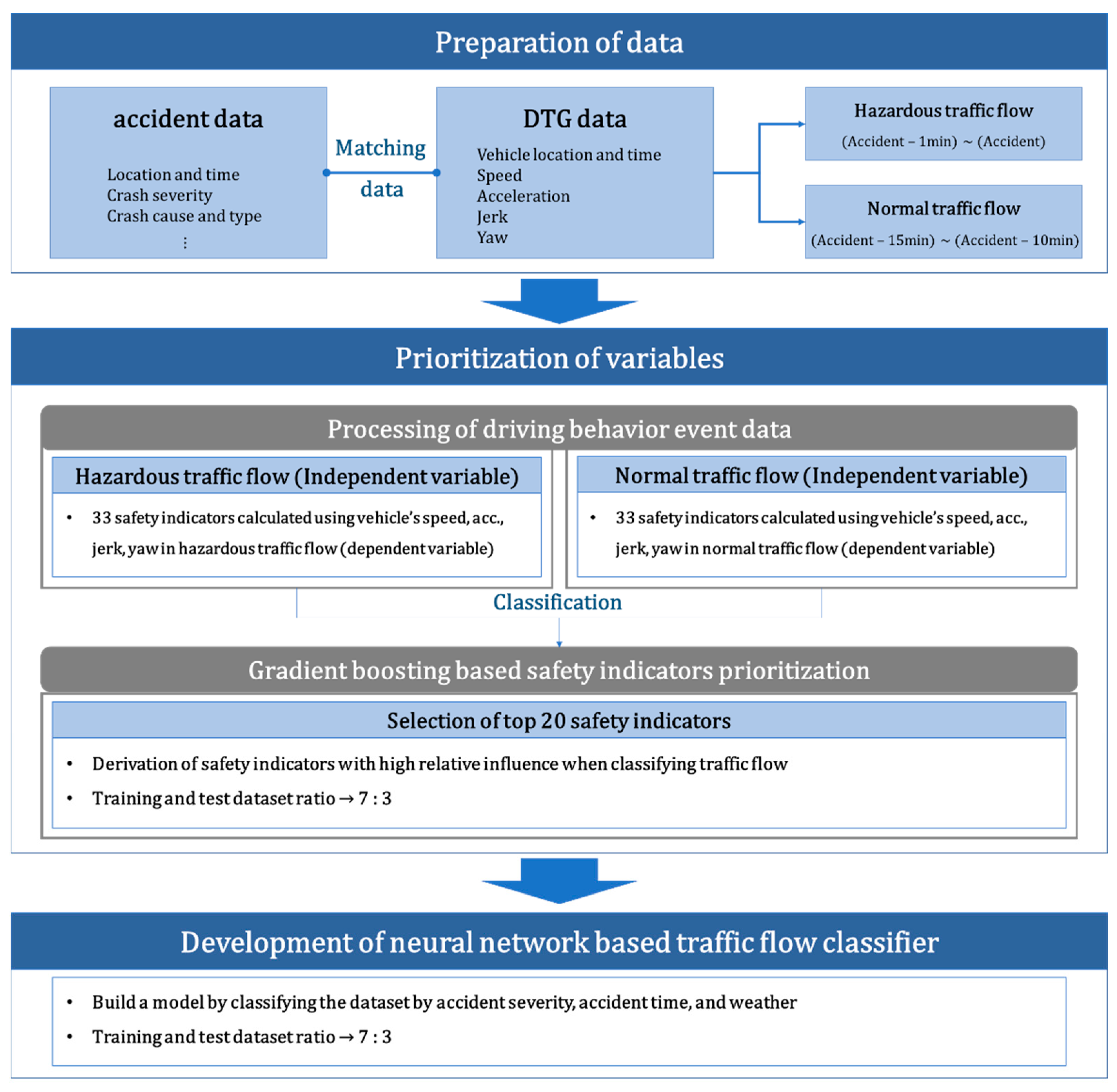
Table 1.
Hyperparameters of gradient boosting.
| Hyperparameters | Definition |
|---|---|
| N tree | Number of tree |
| Interaction depth | The number of branches to extend from each node (the depth of the tree) |
| Shrinkage | Controls how fast the algorithm makes the gradient descent (learning rate) |
Table 2.
Safety indicators.
| Indicator | Variable Name | |
|---|---|---|
| Peak to peak jerk | P to p jerk | |
| SRI | SRI_variable (speed, acc, jerk, yaw) | |
| EDI | EDI_variable (speed, acc, jerk, yaw) | |
| Dangerous driving events rate | Dangerous event | |
| RDEs | RDE | |
| LNJ/LPJ | LNJ/LPJ_threshold | |
| Rapid peak to peak jerk rate | Rapid p to p jerk rate | |
| Yaw rate | Yaw rate | |
| Driving volatility | Standard deviation | S.D_variable (speed, acc, jerk, yaw) |
| Mean absolute deviation | MAD_variable (speed, acc, jerk, yaw) | |
| TVSV (Time-varying stochastic volatility) | TVSV_variable (speed, acc, jerk, yaw) | |
Table 3.
Optimal hyperparameters for gradient boosting.
| Hyperparameters | Optimal Value |
|---|---|
| N tree | 44 |
| Interaction.depth | 5 |
| Shrinkage | 0.05 |
Table 4.
Relative influence of variables.
| Rank | Variable Name | Relative Influence |
|---|---|---|
| 1 | Dangerous event | 33.65 |
| 2 | SRI_yaw | 9.03 |
| 3 | RDEs | 8.33 |
| 4 | TVSV_speed | 4.85 |
| 5 | P to p jerk | 4.07 |
| 6 | MAD_speed | 3.68 |
| 7 | Rapid p to p jerk rate | 3.51 |
| 8 | SRI_acc | 3.49 |
| 9 | S.D_acc | 3.32 |
| 10 | Yaw rate | 3.06 |
| 11 | S.D_yaw | 2.63 |
| 12 | MAD_yaw | 2.51 |
| 13 | SRI_speed | 2.42 |
| 14 | TVSV_acc | 2.37 |
| 15 | LPJ_1.5 | 2.16 |
| 16 | LPJ_2 | 1.84 |
| 17 | S.D_jerk | 1.57 |
| 18 | SRI_jerk | 1.36 |
| 19 | MAD_acc | 1.12 |
| 20 | LPJ_4 | 0.87 |
Table 5.
Optimal hyperparameters for neural network.
| Hyperparameters | Optimal Value |
|---|---|
| Transfer function | Symmetric sigmoid |
| Number of hidden layers | 3 |
| Number of neurons | (30,75,55) |
Table 6.
Classification results of neural network (total data).
| Predicted | |||
|---|---|---|---|
| Normal Traffic Flow | Hazardous Traffic Flow | Correct Classification Rate (%) | |
| Normal traffic flow | 341 | 10 | 97.15 |
| Hazardous traffic flow | 13 | 61 | 82.43 |
| Overall percentage (%) | 94.59 | ||
Table 7.
The number of samples.
| Data Set | Total | Normal Traffic Flow | Hazardous Traffic Flow | |
|---|---|---|---|---|
| Total | 1429 | 1183 | 246 | |
| Severity | D | 1029 | 849 | 180 |
| ABC | 390 | 324 | 66 | |
| D/N | Day | 945 | 790 | 155 |
| Night | 474 | 383 | 91 | |
| Weather | Good | 1101 | 908 | 193 |
| Bad | 299 | 249 | 50 | |
Table 8.
Evaluation of performance for models.
| Data Set | Accuracy | Sensitivity | Specificity | |
|---|---|---|---|---|
| Total | 97.15% | 96.33% | 85.92% | |
| Severity | D | 94.81% | 96.85% | 85.19% |
| ABC | 97.44% | 96.98% | 94.44% | |
| D/N | Day | 93.64% | 96.6% | 79.17% |
| Night | 95.07% | 97.35% | 86.21% | |
| Weather | Good | 94.24% | 96.34% | 84.21% |
| Bad | 95.51% | 97.3% | 86.67% | |
Publisher’s Note: MDPI stays neutral with regard to jurisdictional claims in published maps and institutional affiliations. |
© 2021 by the authors. Licensee MDPI, Basel, Switzerland. This article is an open access article distributed under the terms and conditions of the Creative Commons Attribution (CC BY) license (https://creativecommons.org/licenses/by/4.0/).
Share and Cite
MDPI and ACS Style
Kim, Y.; Park, J.; Oh, C. A Crash Prediction Method Based on Artificial Intelligence Techniques and Driving Behavior Event Data. Sustainability 2021, 13, 6102. https://0-doi-org.brum.beds.ac.uk/10.3390/su13116102
AMA Style
Kim Y, Park J, Oh C. A Crash Prediction Method Based on Artificial Intelligence Techniques and Driving Behavior Event Data. Sustainability. 2021; 13(11):6102. https://0-doi-org.brum.beds.ac.uk/10.3390/su13116102
Chicago/Turabian StyleKim, Yunjong, Juneyoung Park, and Cheol Oh. 2021. "A Crash Prediction Method Based on Artificial Intelligence Techniques and Driving Behavior Event Data" Sustainability 13, no. 11: 6102. https://0-doi-org.brum.beds.ac.uk/10.3390/su13116102
Note that from the first issue of 2016, this journal uses article numbers instead of page numbers. See further details here.