People’s Avoidance of Neighboring Agricultural Urban Green Infrastructure: Evidence from a Choice Experiment

Abstract

This study evaluates people’s preferences regarding the proximity of their residence to agricultural urban green infrastructure (UGI), such as agricultural land and satoyama, and discusses the availability of these types of land as UGI. UGI is vital for reducing the negative environmental impacts of urban areas, as these impacts are too large to ignore. In this study, we conducted an online survey and a choice experiment to investigate people’s perceptions regarding the proximity of their residence to agricultural UGI (AUGI). The respondents of the choice experiment were 802 inhabitants of Ishikawa Prefecture, Japan, which has rich agricultural resources. To examine explicitly the spatial autocorrelation of people’s preferences, in this study, we used the spatial econometrics method. The main empirical findings are that people prefer agricultural land far away from their residence—more than 1000 m, not within 1000 m—which reflects the not-in-my-backyard phenomenon. Meanwhile, people’s preferences regarding proximity to satoyama are complicated and their preferences are positively spatially autocorrelated. The results indicate that policymakers and urban planners should manage and provide AUGI far away from residential areas; otherwise, they must address people’s avoidance of neighboring AUGI.

1. Introduction

The importance of urban green infrastructure (UGI) is gaining recognition in the development and planning of cities. According to Benedict and McMahon (2012), green infrastructure (GI) can be conceptualized as an ecological framework that contributes to environmental, social, and economic sustainability [1]. In addition, according to the European Commission, GI is defined as “strategically planned network of natural and semi-natural areas with other environmental features designed and managed to deliver a wide range of ecosystem services” [2]. Furthermore, Pauleit et al. (2011) define UGI as multifunctional green networks that contribute to promote biodiversity and develop sustainable cities [3]. Despite the various definitions proposed, it is not easy to understand the GI concept succinctly. Nevertheless, as pointed out by Hansen and Pauleit (2014), GI is characterized by a combination of nature conservation and green space planning [4]. Examples of UGI are green spaces, such as public parks and urban forests, and local green objects, such as green roofs and green walls [5,6]. Agricultural land in urban areas is also a form of UGI. UGI has contributed to people’s lives in many ways, for instance, toward a sustainable city [7,8,9], biodiversity conservation [10,11], climate change adaptation [12,13,14,15,16], and the improvement of residents’ living [17,18]. In addition, agricultural land in urban areas has contributed to food production, biodiversity conservation, and enhanced sustainability of urban areas [19,20,21].

However, agricultural UGI (called AUGI hereinafter) has received less attention. Notably, the contributions of agricultural land as UGI have been neglected [6,22]. Previous literature mainly focuses on small, urban agricultural activities, such as urban gardening, and their contributions to society, such as community empowerment or food supply to support subsistence or health [19]. According to Rolf et al. (2019), previous literature has not focused on large agricultural land that might negatively impact people’s health [6]. In addition, less attention is being paid to agricultural land in urban areas because of a lack of knowledge about their value. Many previous studies have evaluated the economic value of UGI and people’s perception of UGI to help policymakers and urban planners effectively manage and provide UGI [5,23,24]. However, as mentioned above, less attention has been paid to agricultural land as UGI in the previous literature. This gap leads to the failure to inform policymakers and urban planners about managing and providing agricultural land as UGI.

Much of the previous literature refers to either the non-use value of agricultural land or willingness to pay (WTP) for agricultural land conservation using the revealed preference and/or the stated preference methods. Previous studies have evaluated the spatial distance between people’s residences and agricultural land using the hedonic price model, e.g., [25,26,27,28,29,30,31,32,33,34]. Ready and Abdalla (2005) reveal that agricultural land within 400 m of a residence has a positive influence on the residence price [33]. Walls et al. (2015) also show that agricultural landscapes that can be viewed from a residence positively influence the residence price [34]. Meanwhile, Hite et al. (2006) find a negative effect of agricultural land on residential prices when situated within 0.25 miles (approximately 402 m) of the residences [28]. Furthermore, Münch et al. (2016) find no effect of agricultural land on residential prices [32]. According to Bergstrom and Ready (2009), as demonstrated in the examples above, findings on the effect of spatial distance between people’s residence and agricultural land differ in the literature, and conclusive results have not been obtained [25].

Previous studies use the stated preference method to evaluate agricultural land. For example, Shoyama et al. (2013) use the conjoint analysis method to evaluate WTP to conserve agricultural land and forests in the Hokkaido Prefecture, Japan [35]. They show that people prefer the conservation of agricultural land. Duke and Ilvento (2004) also evaluate the value of conserving agricultural land and find that this is favorable to the residents of the target area [36]. Yang et al. (2016) use the conjoint analysis method to evaluate the non-use value of agricultural land [37]. They also reveal the positive non-use value of agricultural land and suggest the importance of agricultural land conservation. Meanwhile, the value of agricultural land as UGI has not been discussed.

To consider agricultural land as UGI, it is critical to evaluate the effect of people’s proximity to agricultural land [21]. As mentioned above, agricultural land has both positive and negative impacts, called ecological services and disservices, respectively. Some examples of ecological disservices are allergic reactions, unpleasant smells, injuries by animals, traffic accidents, and criminality induced by poor visibility due to the natural environment in neighboring residential areas [38,39,40]. This negative effect of agricultural land may cause people to develop the attitude called not-in-my-backyard (NIMBY) [41]. People have recognized the importance of such land use for society and the environment but prefer these land uses to exist far from their residence.

It is necessary to evaluate people’s preferences regarding the proximity of their residence to agricultural land for preferable management and provision of agricultural land as UGI, because the NIMBY phenomenon can be strongly influenced by spatial distance, considering the characteristics of the agricultural land. The degree of proximity that people prefer influences the relationship between people and AUGI. If people do not prefer AUGI in their neighbor, it may be necessary to keep them separate from residential areas to obtain public support of environmental protection policies. In other words, policymakers and urban planners must conserve agricultural land in the periphery or outside urban areas if people want to stay away from them.

Some previous studies focus on the proximity of people’s residence to UGI, e.g., [42,43]. Conedera et al. (2015) use a quantitative questionnaire and find that those living near green spaces tend to evaluate their quality of life positively [42]. They also discuss the positive influence of neighboring UGI, citing some studies. However, to the best of our knowledge, no previous study has evaluated people’s preferences regarding the spatial distance between agricultural land and their residence. In this sense, this study contributes to scientific knowledge by investigating people’s preferences regarding the proximity of their residence to agricultural land as UGI, using the stated preference method. This is essential for the application of agricultural land as UGI and ultimately for the development of sustainable cities.

This study evaluates people’s preferences regarding the proximity of their residence to AUGI, such as agricultural land and satoyama, and biodiversity derived from AUGI. For this purpose, a choice experiment is conducted. A spatial econometric model is used to consider explicitly the spatial autocorrelation of people’s environmental preferences, e.g., [44,45,46,47]. Furthermore, based on the results, the application of agricultural land as UGI is discussed.

The remainder of this paper is organized as follows. The following section introduces the materials and methods of the study—the survey design, study area, choice experiment, and estimation strategies. Section 3 presents the estimation results, and the subsequent section provides an overview of the results. The final section presents the conclusions of this study.

2. Materials and Methods

2.1. Study Area

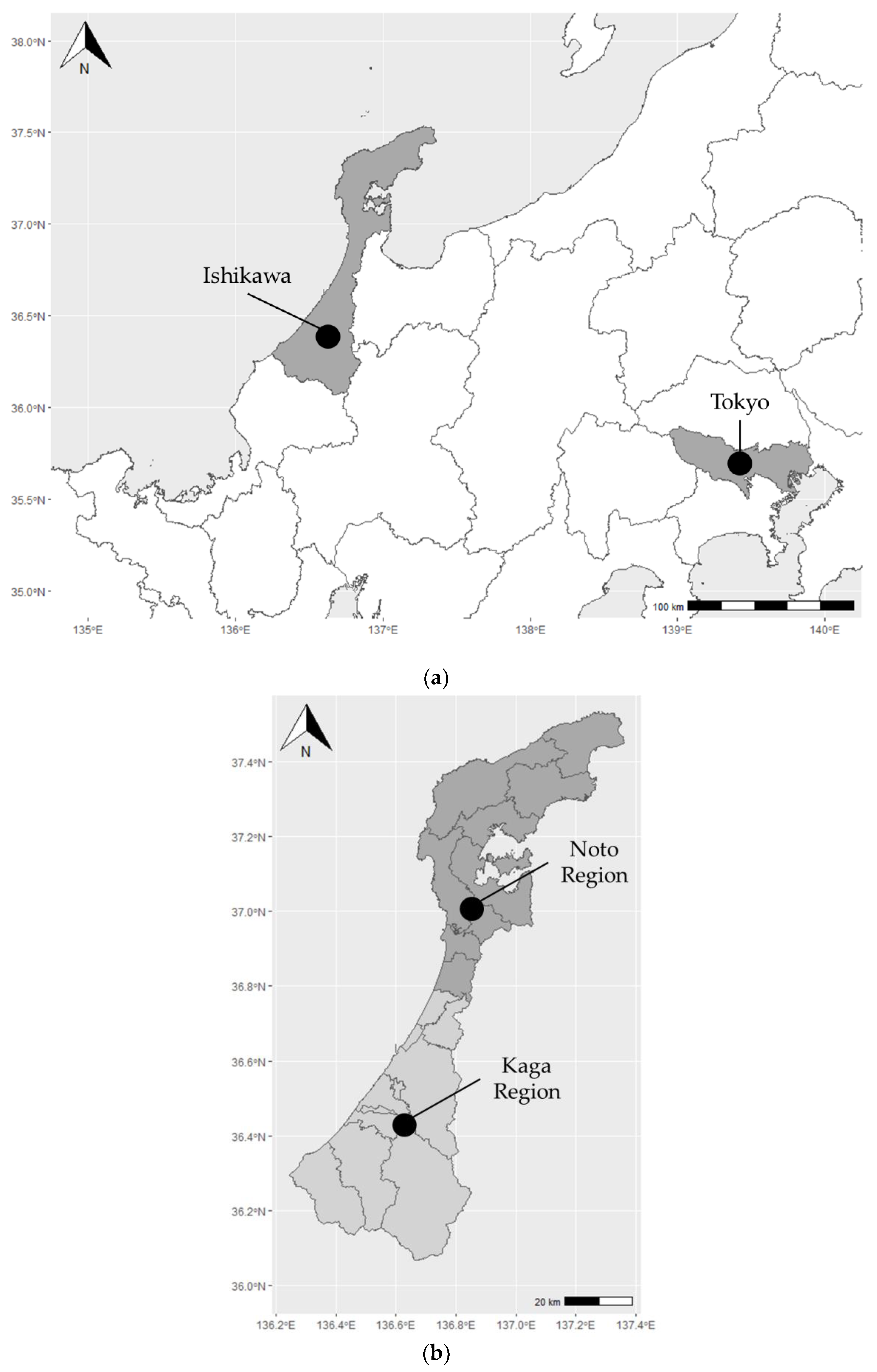
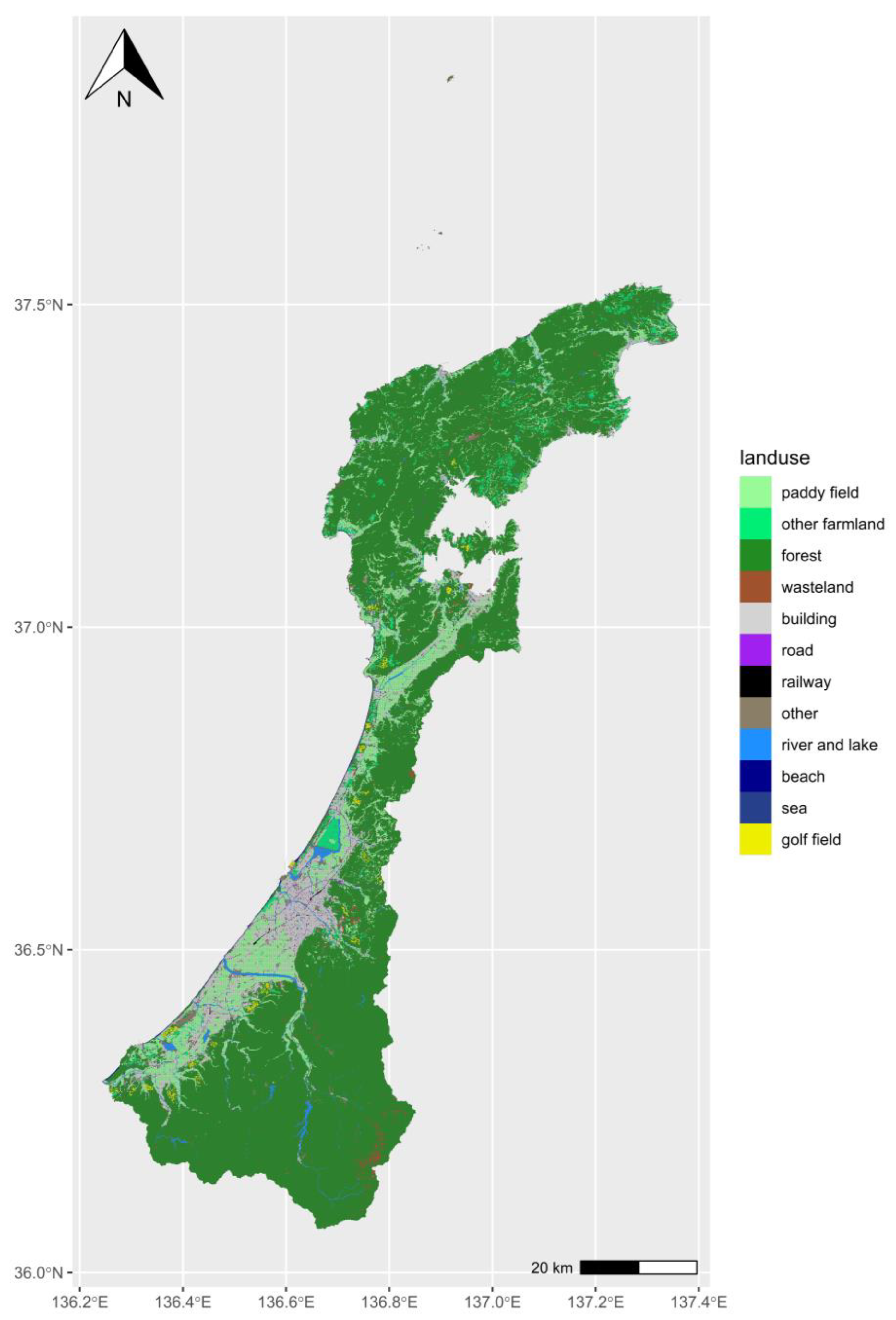
The study area is Ishikawa Prefecture in Japan (see Figure 1 and Figure 2), which is located mid-north of mainland Japan. This prefecture is divided into two regions: the Kaga and Noto regions. Its inhabitants mainly live in the Kaga region because this is where the prefecture capital city, Kanazawa city, is located. Ishikawa Prefecture has approximately 11 million people, and the Noto region had less than 200,000 people in 2015. Figure 1 shows the location of Ishikawa Prefecture. Figure 2 represents the land use pattern of Ishikawa Prefecture.

Ishikawa Prefecture, especially the Noto region, has rich agricultural resources. Geographically, the Noto region consists of many hills, low mountains, and a few flat lands not suitable for agriculture. However, such disadvantages create a unique agricultural landscape called “satoyama”. Satoyama land is a traditional landscape in Japan [48,49,50,51]. It has diverse land uses: agricultural and non-agricultural—cropland, woodland, grassland; for farms, ponds, and brooks. In this sense, satoyama land is a more multifunctional land use system than agricultural land. Satoyama land provides diverse environmental services, such as remarkable sights, traditions, and recreational opportunities. The examples include agricultural landscapes known as terraced rice paddies, traditional religious practices, and agricultural rituals that have been registered as intangible cultural heritage by UNESCO [48].

Satoyama land contributes to biodiversity conservation and climate change mitigation, as well as well-being of human beings. For example, the satoyama in the Noto region is a popular destination for migratory birds, and many endangered species have been observed there. Many of the endangered species observed in satoyama depend on farmland managed by humans, which suggests that satoyama is a form of land use in which humans and nature can coexist.

The main reason for selecting this region as the study site is that it has rich agricultural resources, thus its inhabitants are expected to be familiar with the agricultural context. The Noto region in Ishikawa Prefecture in Japan has valuable agricultural land. This region has been recognized as a “Globally Important Agricultural Heritage System” by the Food and Agriculture Organization in 2011 because of its traditional agricultural landscapes and culture—rituals and practices [49].

2.2. Survey Design

The online survey was conducted on a representative sample of 1648 inhabitants in Ishikawa Prefecture, including the Noto region, from January 27 to 28 and from February 17 to 18 in 2020. The survey was conducted to investigate the inhabitants’ preferences regarding the proximity of their residences to agricultural land. A choice experiment was conducted for this purpose.

The survey comprised 35 questions, including questions about the respondents’ interest in agriculture and the environment (e.g., “Have you ever heard about biodiversity?”), the details of the respondent’s residence (e.g., proximity to the nearest agricultural land/satoyama and monthly rent), choice experiment, and socioeconomic characteristics (see

Table A1. List of questions.

Question	Response Alternatives
Group: Attitudes and ideas about the natural environment
How interested are you in nature?	✓ I am very interested. ✓ Somewhat interested. ✓ Not very interested. ✓ Not at all interested. ✓ I do not know.
What do you think is the best policy for agriculture and rural areas in the future?	✓ National land and environmental conservation. ✓ Economic efficiency and effectiveness ✓ Both ✓ Other ✓ I do not know
How would you like to be involved in rural areas that have lost vitality due to the stagnation of agriculture, depopulation and aging of the population?	✓ I would like to actively visit such areas to help with farming, environmental conservation activities, festivals and other activities to maintain traditional culture. ✓ If I have an opportunity, I would like to visit …. ✓ I would not like to visit …. ✓ Other ✓ I do not know
Have you ever heard about biodiversity?	✓ I know what the word means. ✓ I do not know what that means, but I have heard it before. ✓ I have never heard of it. ✓ I do not know
What do you think about the fact that efforts are being made to protect various living things and the environment in which they live in order to preserve biodiversity?	✓ Even if human life is restricted to some extent, priority should be given to preserving an environment where a wide variety of organisms can live. ✓ Promote conservation of the environment for a wide variety of living things to the extent that human life is not restricted. ✓ To ensure the richness and convenience of human life, it is unavoidable that the environment in which a wide variety of living things can live will be lost. ✓ Other ✓ I do not know
Group: Housing characteristics
Answer the 8-digit number contained within the 1 km × 1 km frame of your location.
What is the floor plan of the house you are currently living in?
What is the type of house in which you currently live?	✓ Detached house. ✓ Large apartment. ✓ Small apartment.
What is the area of the house?
How old is your house? (as of 2020)
What floor do you live on?
What is the distance from where you live to the nearest train station?	Approximately     minutes by (walk, bicycle, car, or public transport).
What is the distance from your place of residence to the nearest shopping mall?	Approximately     minutes by (walk, bicycle, car, or public transport).
What is the distance from your place of residence to the nearest school?	Approximately     minutes by (walk, bicycle, car, or public transport).
What is the distance from your place of residence to the nearest park?	Approximately     minutes by (walk, bicycle, car, or public transport).
What is the distance from your place of residence to the nearest hospital?	Approximately     minutes by (walk, bicycle, car, or public transport).
The respondent’s housing demographics	✓ Live in an apartment. ✓ Owned residences. ✓ Owned residences and had already finished paying the house mortgage
Monthly rent	1: –29,999; 2: 30,000–34,999; …;20: 120,000–
Proximity to agricultural land	1: 0 m; 2: 200 m; 3: 500 m; 4: 1000 m; 5: more than 1000 m
Proximity to satoyama	1: 0 m; 2: 200 m; 3: 500 m; 4: 1000 m; 5: more than 1000 m
Most preferred proximity to agricultural land	1: 0 m; 2: 200 m; 3: 500 m; 4: 1000 m; 5: more than 1000 m
Most preferred proximity to satoyama	1: 0 m; 2: 200 m; 3: 500 m; 4: 1000 m; 5: more than 1000 m
Group: Choice experiment 1–8
Group: Socio-economic characteristics
What is your zip code?
How many years have you lived in the area where you currently reside?
What is your occupation?	Employee; Public servant; Student; Self-employed; Agriculture, forestry and fishery workers; Homemaker; Part-time job; Pensioner; Others
Please indicate your household’s annual income (including tax).	1: –200; 2: 200–399; …; 8: 1400–
Please indicate the number of people in your household (including you).

Note: All questions were provided in Japanese.

in Appendix A for the list of all the questions). Regarding monthly rent, there were three different questions, depending on the respondent’s demographics. Those who lived in an apartment were asked about their monthly rent. Those who lived in owned residences were asked about their monthly house mortgage payments. Those who lived in owned residences and had already finished paying the house mortgage were asked about their monthly real property tax, which was treated as their monthly rent.

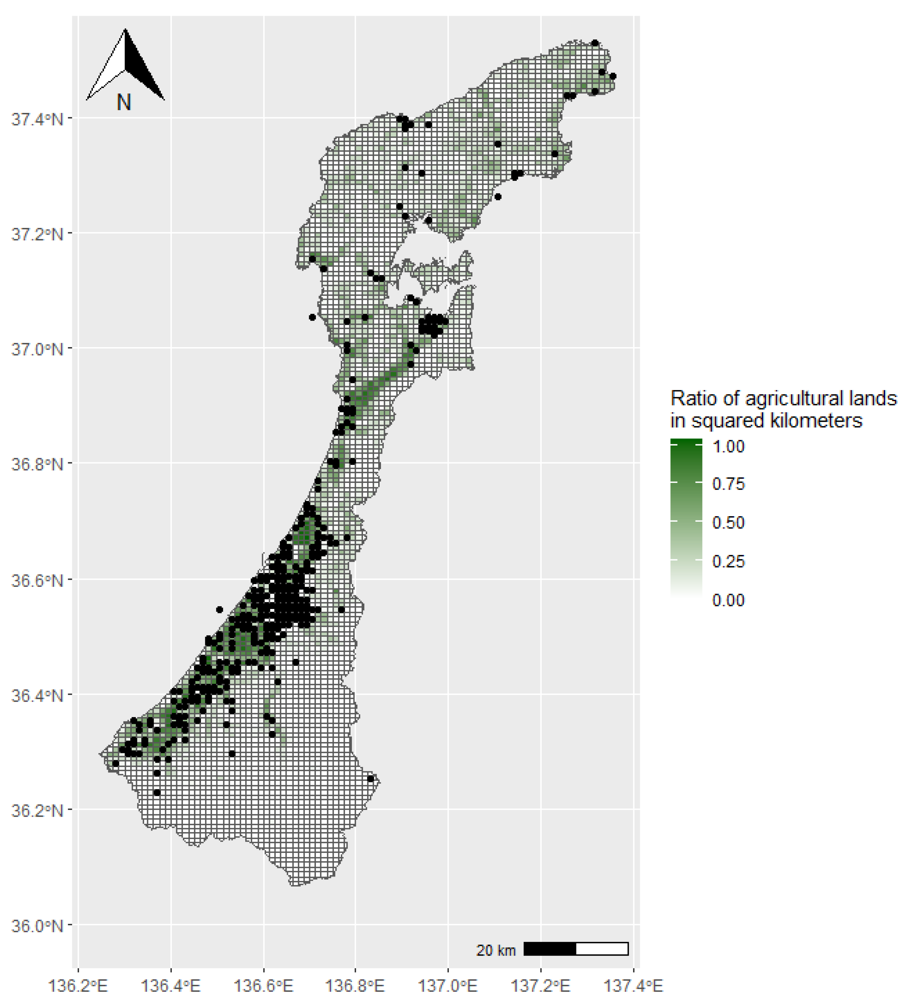
The survey was also designed to consider the spatial autocorrelation of people’s preferences. All the respondents were asked to report the 1 km by 1 km parcel on a given map (see Figure 3) that indicates their residence. Some respondents refused to provide this information. They were excluded from the sample, and 802 valid respondents were finally obtained. The respondents’ characteristics are summarized in

Table 1. Summary of the valid respondents’ characteristics.

Variable	Definition	N	Min	Mean	Max	S.D.
Sex	0: female; 1: male	802	0	0.52	1	0.50
Age (year)	1: 18–19; 2: 20–29; …; 7: 70–79; 8: 80–89	802	1	4.05	8	1.38
Living year (year)	Years lived in the current city	802	0	23.44	82	18.27
Income (JPY 10,000)	1: –200; 2: 200–399; …; 8: 1400–	802	1	3.30	8	1.60
Monthly rent (JPY)	1: –29,999; 2: 30,000–34,999; …; 20: 120,000–	802	0	5.73	20	5.01
Proximity to agricultural land	Respondent’s subjective proximity to agricultural land 1: 0 m; 2: 200 m; 3: 500 m; 4: 1000 m; 5: more than 1000 m	802	1	3.29	5	1.39
Proximity to satoyama	Respondent’s subjective proximity to satoyama 1: 0 m; 2: 200 m; 3: 500 m; 4: 1000 m; 5: more than 1000 m	802	1	4.31	5	1.07

(see

Table A2. Summary of all the respondents’ characteristics.

Variable	Definition	N	Min	Mean	Max	S.D.
Sex	0: female; 1: male	1648	0	0.49	1	0.50
Age (year)	1: 18–19; 2: 20–29; …; 7: 70–79; 8: 80–89	1648	1	4.05	8	1.39
Living year (year)	Years lived in the current city	1643	0	23.46	82	18.27
Income (JPY 10,000)	1: –200; 2: 200–399; …; 8: 1400–	1648	1	3.16	8	1.60
Monthly rent (JPY)	1: –29,999; 2: 30,000–34,999; …; 20: 120,000–	1648	0	5.70	20	5.03
Proximity to agricultural land	Respondent’s subjective proximity to agricultural land 1: 0 m; 2: 200 m; 3: 500 m; 4: 1000 m; 5: more than 1000 m	1648	1	3.36	5	1.39
Proximity to satoyama	Respondent’s subjective proximity to satoyama 1: 0 m; 2: 200 m; 3: 500 m; 4: 1000 m; 5: more than 1000 m	1634	1	4.25	5	1.13

in Appendix A for all respondents’ characteristics).

2.3. Choice Experiment

The survey’s choice experiment was designed to investigate people’s preferences regarding the (1) proximity of their residence to agricultural land/satoyama and (2) biodiversity derived from AUGI. The choice experiment comprised a variety of conjoint analyses capable of eliciting the respondents’ tastes for multiple attributes [52]. The respondents had to choose their preferred alternatives, and these choices were repeated as a series of choice tasks. This method can evaluate the respondents’ preferences for various attributes that affect their decisions.

In the choice experiment, four attributes were used to describe the hypothetical residence: proximity to an agricultural piece of land, proximity to a satoyama area, the number of observable dragonfly species around the residence, and monthly rent (JPY).

Four levels were used for the proximity to agricultural land attribute: 0 m, 200 m, 500 m, and 1000 m. These four levels were assigned because people may not care about the environment too far away from their residence. In addition, observable agricultural landscapes may influence people’s preferences [28,33,34].

Four levels were used for the proximity to satoyama attribute: 0 m, 200 m, 500 m, and 1000 m. The main reason for using satoyama as a type of land use is that, as mentioned above, satoyama is a more complex and valuable landscape compared with agricultural land. Therefore, people’s preference for satoyama might also be more complex than that for agricultural land.

Four levels were used for the attribute number of observable dragonfly species around the residence: 0, 2, 4, and 8 species. This attribute indicates the degree of biodiversity around the respondents’ residence. According to previous studies, the number of dragonfly species can be used as a proxy for the degree of biodiversity, e.g., [50,53,54]. This attribute is used to investigate people’s perceptions of biodiversity around their residence. According to previous studies, people tend to have a positive perception of biodiversity [35,55,56]. However, previous studies that evaluate biodiversity tend to consider biodiversity in specific areas with rich nature, such as wetland, forests, and riversides, and they do not evaluate biodiversity in close proximity to people’s daily activities, including people’s residences. It is expected that people might have a different preference for biodiversity around their residences compared with other areas.

The monthly rent in the choice experiment differs among the respondents; this emulates a feasible hypothetical residence choice. Before conducting the choice experiment, the respondents were asked about the actual monthly rent for their residence. Five different monthly rent levels were used in the choice experiment that depended on the respondent’s current monthly rent: 80%, 90%, 100%, 110%, and 120% of the monthly rent. The respondents’ corresponding monthly rent is presented in

Table 2. The respondents’ current monthly rent and corresponding five hypothetical monthly rent.

Current Monthly Rent (JPY)	80%	90%	100%	110%	120%
Less than 30,000	24,000	27,000	30,000	33,000	36,000
30,000–35,000	26,000	29,250	32,500	35,750	39,000
35,000–40,000	30,000	33,750	37,500	41,250	45,000
40,000–45,000	34,000	38,250	42,500	46,750	51,000
45,000–50,000	38,000	42,750	47,500	52,250	57,000
50,000–55,000	42,000	47,250	52,500	57,750	63,000
55,000–60,000	46,000	51,750	57,500	63,250	69,000
60,000–65,000	50,000	56,250	62,500	68,750	75,000
65,000–70,000	54,000	60,750	67,500	74,250	81,000
70,000–75,000	58,000	65,250	72,500	79,750	87,000
75,000–80,000	62,000	69,750	77,500	85,250	93,000
80,000–85,000	66,000	74,250	82,500	90,750	99,000
85,000–90,000	70,000	78,750	87,500	96,250	105,000
90,000–95,000	74,000	83,250	92,500	101,750	111,000
95,000–100,000	78,000	87,750	97,500	107,250	117,000
100,000–105,000	82,000	92,250	102,500	112,750	123,000
105,000–110,000	86,000	96,750	107,500	118,250	129,000
110,000–115,000	90,000	101,250	112,500	123,750	135,000
115,000–120,000	94,000	105,750	117,500	129,250	141,000
More than 120,000	96,000	108,000	120,000	132,000	144,000

.

Finally, lambda is not an attribute but the estimated coefficient of the spatial weight matrix, as described later. Lambda takes a value between −1 and 1. If it is a positive/negative value in our estimation model, people’s preferences are positively/negatively spatially autocorrelated. Lambda that is closer to 1 indicates a stronger positive spatial correlation, and a value closer to −1 indicates a stronger negative spatial correlation. The attributes and levels are listed in

Table 3. The attributes and levels for the choice experiment.

Attributes	Levels
Proximity to agricultural land	0 m, 200 m, 500 m, and 1000 m
Proximity to satoyama	0 m, 200 m, 500 m, and 1000 m
Number of dragonfly species observable around the residence	0, 2, 4, and 8 species
Monthly rent	80%, 90%, 100%, 110%, and 120% of the actual monthly rent

.

For the choice experiment, 36 sets of questions were created using Ngene [57], considering D-efficiency. A D-efficient design allows us to obtain more statistically efficient results compared with the common orthogonal design. The 36 sets were equally divided into six versions, and the respondents were randomly assigned to one of the six versions. The choice experiment question was then repeated six times for each respondent. The respondents were asked to select their preference among the three alternative residences or refuse to choose (i.e., “do not choose among them”).

Answering “do not choose among them” implies that the respondent prefers his/her current residence to the three hypothetical residences he/she faces. Therefore, assumptions must be made about the attributes of the respondent’s actual residence to evaluate such decisions. Proximity to the agricultural land/satoyama perceived by the respondents—asked in the online survey—was applied to the proximity to agricultural land/satoyama attributes. The number of dragonfly species observable around the residence attribute was calculated using the respondent’s parcel and the Satoyama Index [50]. Following Kadoya and Washitani (2011), the number corresponding to the richness of the dragonfly species in a parcel was calculated using the following formula:

$$y_i=\exp \left(0.429x_i+0.735\right)$$

(1)

where $y_i$ is the number corresponding to the richness of the dragonfly species in parcel $i$, and $x_i$ is the satoyama index in parcel $i$ [50]. Finally, the actual monthly rent for a residence was applied to the monthly rent attribute. The variables for estimation and its definitions are provided in

Table 4. Variables for estimation and their definitions.

Variables	Definitions
Proximity to agricultural land
PROXAGRI0 (base)	Dummy variable: the distance between a respondent’s residence and a piece of agricultural land is 0 m
PROXAGRI200	Dummy variable: the distance between a respondent’s residence and a piece of agricultural land is 200 m
PROXAGRI500	Dummy variable: the distance between a respondent’s residence and a piece of agricultural land is 500 m
PROXAGRI1000	Dummy variable: the distance between a respondent’s residence and a piece of agricultural land is 1000 m
PROXAGRIover1000	Dummy variable: the distance between a respondent’s residence and a piece of agricultural land is more than 1000 m
Proximity to a satoyama area
PROXSATO0 (base)	Dummy variable: the distance between a respondent’s residence and a satoyama area is 0 m
PROXSATO200	Dummy variable: the distance between a respondent’s residence and a satoyama area is 200 m
PROXSATO500	Dummy variable: the distance between a respondent’s residence and a satoyama area is 500 m
PROXSATO1000	Dummy variable: the distance between a respondent’s residence and a satoyama area is 1000 m
PROXSATOover1000	Dummy variable: the distance between a respondent’s residence and a satoyama area is more than 1000 m
Number of dragonfly species observable around the residence
BIODIV0 (base)	0 species can be observed around the respondent’s residence
BIODIV2	2 species can be observed around the respondent’s residence
BIODIV4	4 species can be observed around the respondent’s residence
BIODIV8	8 species can be observed around the respondent’s residence
Monthly rent	80%, 90%, 100%, 110%, and 120% of the current monthly rent
Lambda	Coefficient of the spatial weight matrix

Note: The PROXAGRIover1000 and PROXSATOover1000 variables were used to describe the attribute of the respondent’s actual residence when he/she selected “do not choose among them”.

, and

Table 5. An example of the choice experiment.

Attribute	Choice 1	Choice 2	Choice 3	Choice 4
Proximity to a piece of agricultural land	200 m	500 m	0 m	Do not choose among them
Proximity to a satoyama area	1000 m	0 m	1000 m
Number of observable dragonfly species	0 species	8 species	0 species
Monthly rent	110%	90%	100%
Choose the Most Preferred Option	☑	☐	☐	☐

is an example of the choice experiment we conducted.

2.4. Estimation Strategy

A hierarchical Bayes estimation of a random parameter logit model with spatial autocorrelation was used as the estimation model to consider the spatial autocorrelation of people’s preferences, which affected the estimation results. According to Train (2009), Bayesian models have some advantages over traditional maximum likelihood methods [58]. For example, Bayesian models can deal with outliers and heteroscedasticity [59], and they can avoid computational difficulties caused mainly by the sample size.

The basic idea is based on the random utility models. In the choice model, it is assumed that individuals receive utility according to their choices in the choice experiment, and their choices maximize their utility:

$$U_{njt}=X_{njt}{\beta }_n+{\epsilon }_{njt}$$

(2)

where $n\in \left(1,\cdots ,N\right)$ is the index of respondents,$j\in \left(1,\cdots ,J\right)$ is the index of alternatives, $t\in \left(1,\cdots ,T\right)$ is the index of tasks in the choice experiment, $U_{njt}$ is the utility, $X_{njt}$ is the band of attributes and ${\epsilon }_{njt}$ is the random draw from a Type I extreme value distribution. ${\beta }_n$ is the coefficient vector of the individual taste parameter, which is assumed to be normally distributed (${\beta }_n ~ N\left(b, \eta \right)$). Considering the spatial autocorrelation, $\mathbf{\beta }$ can be arranged as follows:

$$\mathbf{\beta }=\lambda W\beta +b+\eta ={\left(I-\lambda W\right)}^{-1}\left(b+\eta \right)$$

(3)

where $\mathbf{\beta }=\left\{{\beta }_1,\cdots ,{\beta }_N\right\}$ is the matrix of taste parameters, $I$ is the identity matrix, $W$is the spatial weight matrix discussed below, $\lambda$ and $b$ are estimated parameters and $\eta$ is the vector of random draws from $N\left(0,\mathsf{\Sigma }\right)$. Conditional on ${\beta }_n$, the probability of respondent $n$’s series of observed choices in the experiment can be written as a standard logit formula as follows:

$$L(y_n|{\beta }_n)={\displaystyle \prod }_t\left(\raisebox{1ex}{$e^{{\beta }_n^{\prime }{x}_{nit}}$}\!\left/ \!\raisebox{-1ex}{${{\displaystyle \sum }}_j{\beta }_n^{\prime }{x}_{njt}$}\right.\right)$$

(4)

The unconditional probability is the integral of $L\left(y_n\right|{\beta }_n)$ over all values of ${\beta }_n$ weighted by the density of ${\beta }_n$:

$$L_n(y_n|b, \eta )={\displaystyle \int }L(y_n|{\beta }_n)g({\beta }_n|b, \eta )d\eta$$

(5)

where $g(.)$ is the normal distribution that has mean $b$ and variance $\eta$.

According to Train (2009, Chapter 12), the spatial autocorrelation of the random parameter in Equation (3) requires the individual parameters of each respondent, which can be estimated using hierarchical Bayes [58]. It is assumed that the prior distribution of $b$ is a normal distribution with mean zero and a sufficiently large variance, and that $\eta$ is an inverted Wishart distribution with K degrees of freedom for estimation.

Using the prior distributions, the joint posterior distribution on ${\beta }_n\forall n,b, \eta$ can be written as:

$$\mathsf{\Lambda }({\beta }_n\forall n,b, \eta |Y) \propto {\displaystyle \prod }_{n}L(y_n|{\beta }_n)g({\beta }_n|b, \eta )k\left(b, \eta \right)$$

(6)

where $k(.)$ is the prior distribution of $b$ and $\eta$.

Hierarchical Bayes obtains posterior distributions using the Gibbs sampling method [58,60]. The Gibbs sampling method follows three steps: (1) draw from $b|\mathsf{\Sigma }, {\beta }_n$, (2) draw from $\mathsf{\Sigma }|b, {\beta }_n$, (3) draw from${\beta }_n|b, \mathsf{\Sigma }$, and (4) repeat (1)–(3) until convergence. In the Gibbs sampling of this study, the first 10,000 iterations were discarded as burn-in and retained every tenth draw after convergence to reduce the amount of correlation among the consecutive draws. Finally, 2000 draws were obtained from posterior distributions.

In Equation (3), the spatial weight matrix $W$ has an important role in the spatial models. This matrix implicitly defines spatial contiguity among all pairs of respondents. This weight matrix consists of an element $w_{ij}$, and each element weighs the degree of spatial adjacency. Element $w_{ij}$ is binary, indicating whether respondents $i$ and $j$ are adjacent in the simplest case. However, there are no golden rules for choosing the “correct” spatial weight matrix, although this matrix influences the estimation results [61]. In the previous literature, Euclidean distance, economic distance, and social network were used to create a spatial weight matrix, in addition to spatial adjacency, e.g., [29,61,62].

In this study, following Kostov (2010), the Euclidean distance was used to substitute the spatial connection between each respondent [63]. Kostov (2010) points out that the exogeneity of the spatial weight matrix can be considered by using the Euclidean distance for the spatial weight matrix [63].

The operation to define the spatial weight matrix for this study is as follows. The parcels obtained through the online survey indicate the respondents’ residence locations. The Euclidean distance $d_{ij}$ between respondents $i$ and $j$ is defined by calculating the Euclidean distance between the centers of each parcel. When respondents $i$ and $j$ live in the same parcel, the expected Euclidean distance is used based on the assumption of a random location with a uniform distribution; $d_{ij}=0.5214$ following Equation (7):

$$\begin{gathered} P\left[\left|X_1-X_2\right|\le x\right]=1-{\left(1-x\right)}^2=2x-x^2 \\ f\left(x\right)=\{\begin{array}{cc}2\left(1-x\right)& 0\le x\le 1\\ 0& \mathrm{otherwise}\end{array} \\ \mathrm{E}\left[d\right]={{\displaystyle \int }}_0^1{{\displaystyle \int }}_0^{1}4\left(1-x\right)\left(1-y\right){\left(x^2+y^2\right)}^{0.5}dxdy \\ =\frac{1}{15}\left(2+\sqrt{2}+5\ln \left(1+\sqrt{2}\right)\right)=0.5214054\dots \end{gathered}$$

(7)

The choice of $W$ is vital for considering spatial autocorrelation [64,65]. Kostov (2010) also suggests that a popular definition of the spatial weight matrix uses the inverse distance raised to some power [63]. We follow this suggestion and create two spatial weight matrixes based on inverse distance and inverse squared distance as Equations (8) and (9) to ensure the robustness of the estimation result.

$$w_{ij}=1/d_{ij}^2$$

(8)

$$w_{ij}=1/d_{ij}$$

(9)

3. Results

Table 6. Estimation results for the three models.

	Model (A)		Model (B)		Model (C)
Variables	Mean	S.D.	Mean	S.D.	Mean	S.D.
PROXAGRI200	0.623	0.083	0.663	0.151	0.418	0.213
	(0.425–0.769)		(0.318–0.869)		(0.117–0.748)
PROXAGRI500	0.486	0.085	0.712	0.050	0.546	0.132
	(0.309–0.643)		(0.614–0.800)		(0.344–0.787)
PROXAGRI1000	−0.032	0.081	0.315	0.085	0.025	0.254
	(−0.196–0.110)		(0.119–0.448)		(−0.544–0.474)
PROXAGRIover1000	0.609	0.112	0.981	0.069	1.010	0.126
	(0.352–0.804)		(0.859–1.120)		(0.744–1.240)
PROXSATO200	0.763	0.078	1.280	0.117	0.613	0.155
	(0.642–0.919)		(1.100–1.463)		(0.343–0.876)
PROXSATO500	1.140	0.087	1.050	0.093	1.480	0.069
	(1.003–1.323)		(0.812–1.219)		(1.356–1.612)
PROXSATO1000	0.779	0.087	0.681	0.118	1.040	0.085
	(0.624–0.962)		(0.380–0.857)		(0.882–1.224)
PROXSATOover1000	0.211	0.139	0.158	0.044	−0.017	0.173
	(−0.027–0.501)		(0.073–0.249)		(−0.339–0.239)
BIODIV2	−0.259	0.065	−0.438	0.210	−0.442	0.143
	(−0.413–−0.152)		(−0.886–−0.077)		(−0.758–−0.215)
BIODIV4	−0.039	0.060	0.311	0.162	0.198	0.044
	(−0.168–0.068)		(0.074–0.669)		(0.123–0.294)
BIODIV8	−0.475	0.112	−0.368	0.115	−0.304	0.143
	(−0.694–−0.283)		(−0.656–−0.241)		(−0.792–−0.118)
Monthly rent (JPY 1000)	−0.178	0.011	−0.182	0.085	−0.127	0.133
	(−0.202–−0.160)		(−0.440–−0.076)		(−0.444–0.078)
LAMBDA			0.535	0.277	0.275	0.151
			(0.133–1.069)		(0.038–0.592)
Spatial weight matrix	-		$1/d_{ij}^2$		$1/d_{ij}$
Number of individuals	802		802		802
Number of observations	6416		6416		6416
Log-likelihood	−4854.116		−8712.862		−8866.610
Root likelihood	0.503		0.260		0.250

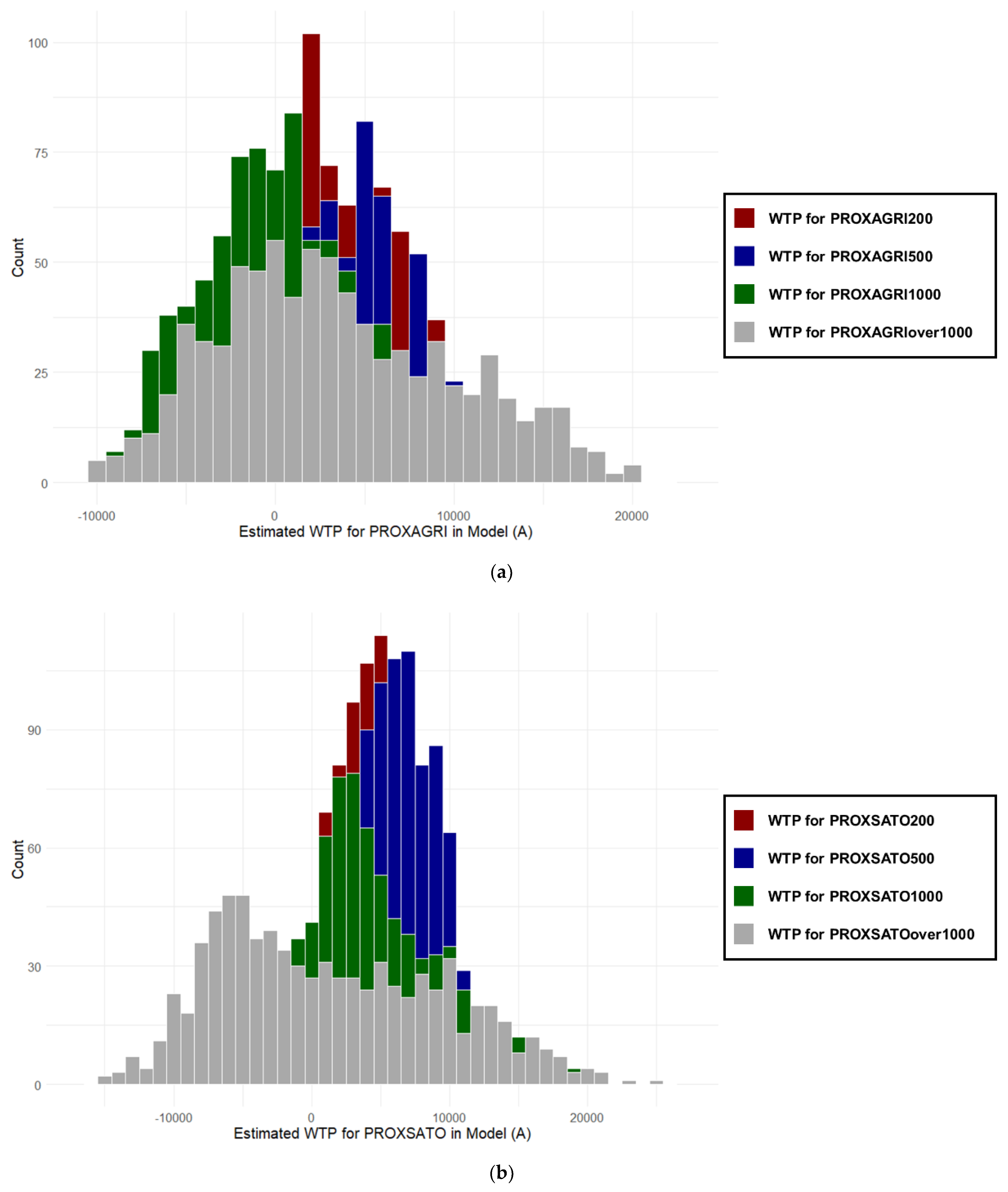
Note: The first 10,000 iterations were discarded as burn-in, and every tenth draw was retained after convergence, for a total of 2000 draws from the posterior. S.D. indicates the standard division of the estimated parameters. The brackets display the minimum and maximum estimated parameters (min–max).

provides the three estimation results from the hierarchical Bayes model, including a non-spatial model and two spatial models; Table 6, and Figure 4, Figure 5 and Figure 6 represent the estimated WTP and the distribution of the estimated WTP based on all the models. Model (A), as the basic model, does not include spatial aspects for comparison with the two spatial models. Models (B) and (C) explicitly consider spatial autocorrelation in people’s preferences. Model (B) uses a spatial weight matrix based on the inverse squared distance (Equation (8)), and Model (C) uses it based on the inverse distance (Equation (9)).

First, we focus on the overall estimation results. All estimation models obtain the expected results, except for BIODIV variables, and quite similar results for most of the variables. In terms of model fit, considering log-likelihood, and root likelihood, Model (A) shows the best model fit (log-likelihood is −4854.116 and root likelihood is 0.503) compared with Models (B) and (C)—the log-likelihood is −8712.862 and −8866.610, and the root likelihood is 0.26 and 0.25, respectively. As seen in Figure 4, Figure 5 and Figure 6, Models (B) and (C) obtain more convergent results compared with Model (A) in terms of estimated WTP. This difference may be due to spatial autocorrelation in people’s preferences.

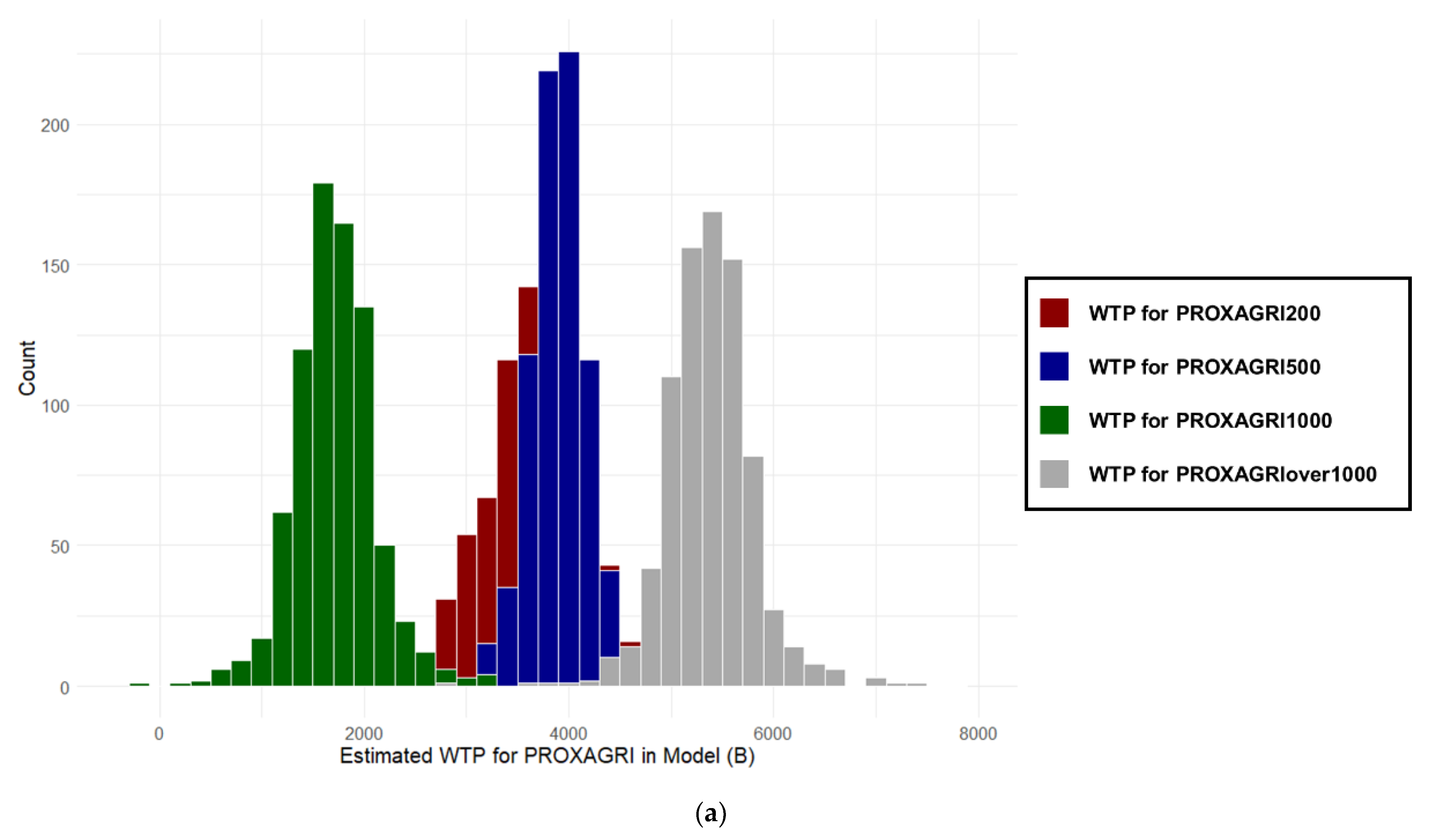
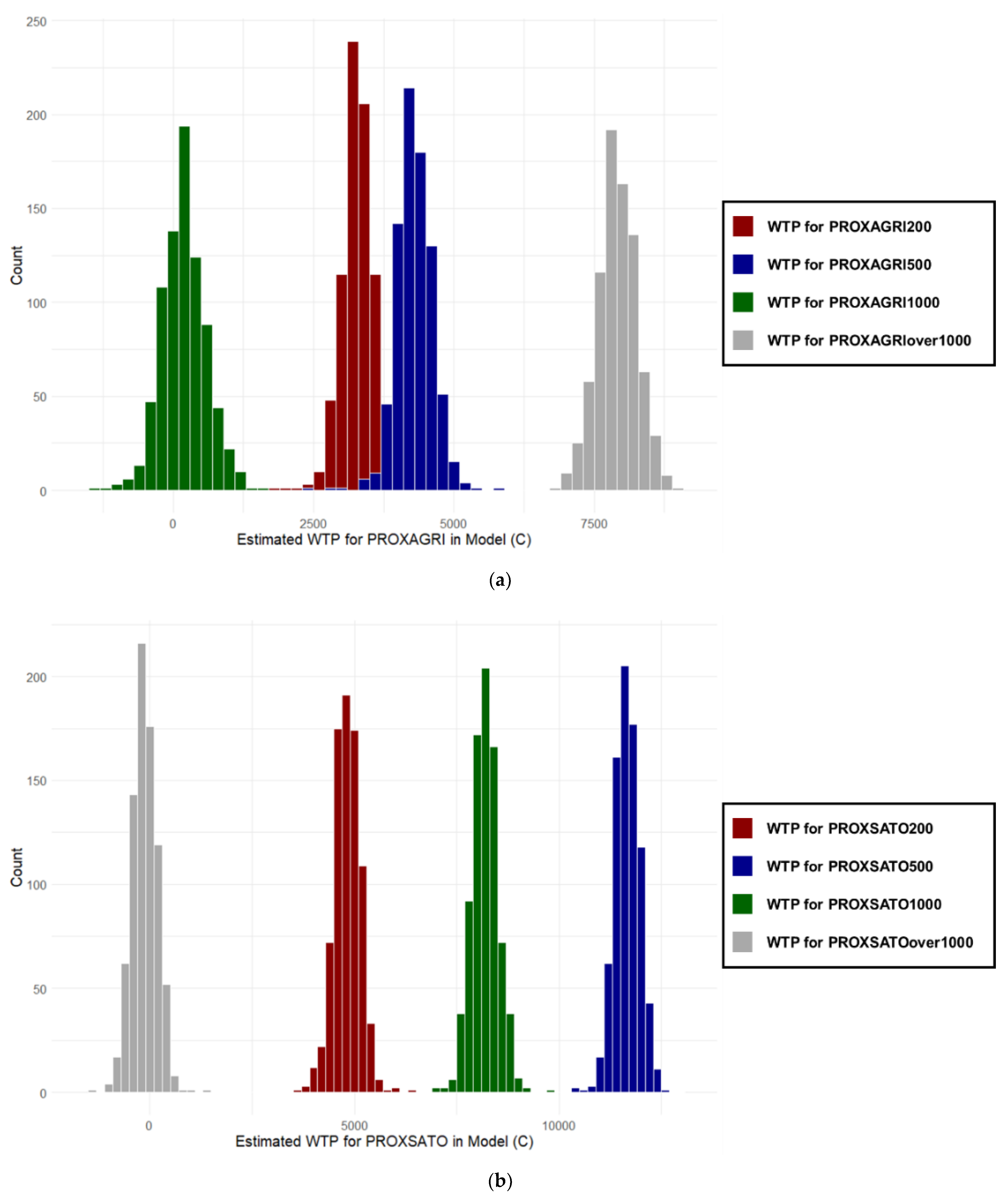
For PROXAGRI—the variables of proximity to agricultural land—all the variables are expected to show a positive coefficient compared with the base variable (PROXAGRI0). In addition, the coefficient of PROXAGRI200 is expected to be the least preferred, and PROXAGRIover1000, the most preferred, based on the NIMBY phenomenon. The estimation results show that all the variables except for PROXAGRI1000 have a positive mean coefficient and do not contain zero in the intervals for all the models. Furthermore, as predicted, PROXAGRI200 is the least preferred, and PROXAGRIover1000 is the most preferred in Models (B) and (C) (see Table 6 and

Table 7. Estimated mean WTPs (in JPY).

Variables	Model (A)	Model (B)	Model (C)
PROXAGRI200	3509	3639	3291
PROXAGRI500	2741	3907	4293
PROXAGRI1000	−182	1731	193
PROXAGRIover1000	3427	5380	7912
PROXSATO200	4301	7013	4818
PROXSATO500	6408	5775	11660
PROXSATO1000	4386	3729	8191
PROXSATOover1000	1220	865	−130
BIODIV2	−1459	−2409	−3483
BIODIV4	−215	1707	1557
BIODIV8	−2681	−2020	−2396

Note: The estimated WTPs are calculated using the price parameter (monthly rent at JPY 1000) and the mean of each estimated parameter.

). For PROXAGRI200 and PROXAGRIover1000, the estimated WTPs are JPY 3639 and 3291 in Models (B) and (C), respectively. By contrast, for Model (A), the results differ. PROXAGRI200 is the most preferred and not PROXAGRIover1000 as predicted. For PROXAGRI200 and PROXAGRIover1000, the estimated WTPs are JPY 3509 and 3427, respectively (see Table 7).

For PROXSATO—the proximity to satoyama variables—all the variables are predicted to show a positive coefficient compared with the base variable (PROXSATO0), and the coefficient of PROXSATO200 is expected to be the least preferred, and PROXSATOover1000 the most preferred, based on the NIMBY phenomenon, similar to the variables related to proximity to agricultural land. Additionally, considering the complexity of satoyama land use, the NIMBY phenomenon functions more intensely, and PROXSATO is expected to be less preferred than PROXAGRI. The estimation results show that all the variables except for PROXSATOover1000 have a positive mean coefficient and do not contain zero in the intervals for all the models. Moreover, PROXSATO200 is the least preferred in Models (A) and (C), as expected. Table 7 shows that the estimated WTP is JPY 4301 and 4818, respectively. In addition, when comparing the WTPs between the PROXSATO and PROXAGRI variables, all WTPs for the PROXSATO variables except for PROXSATOover1000 are larger than those for the PROXAGRI variables, as expected.

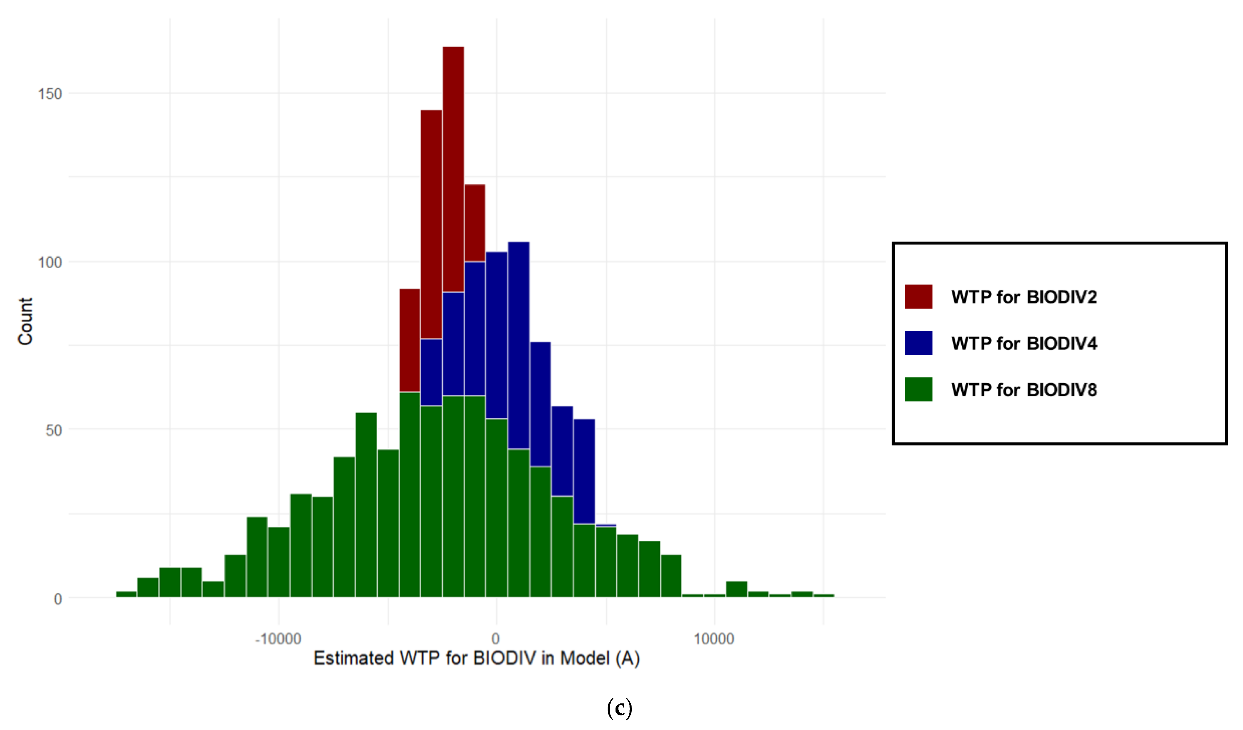
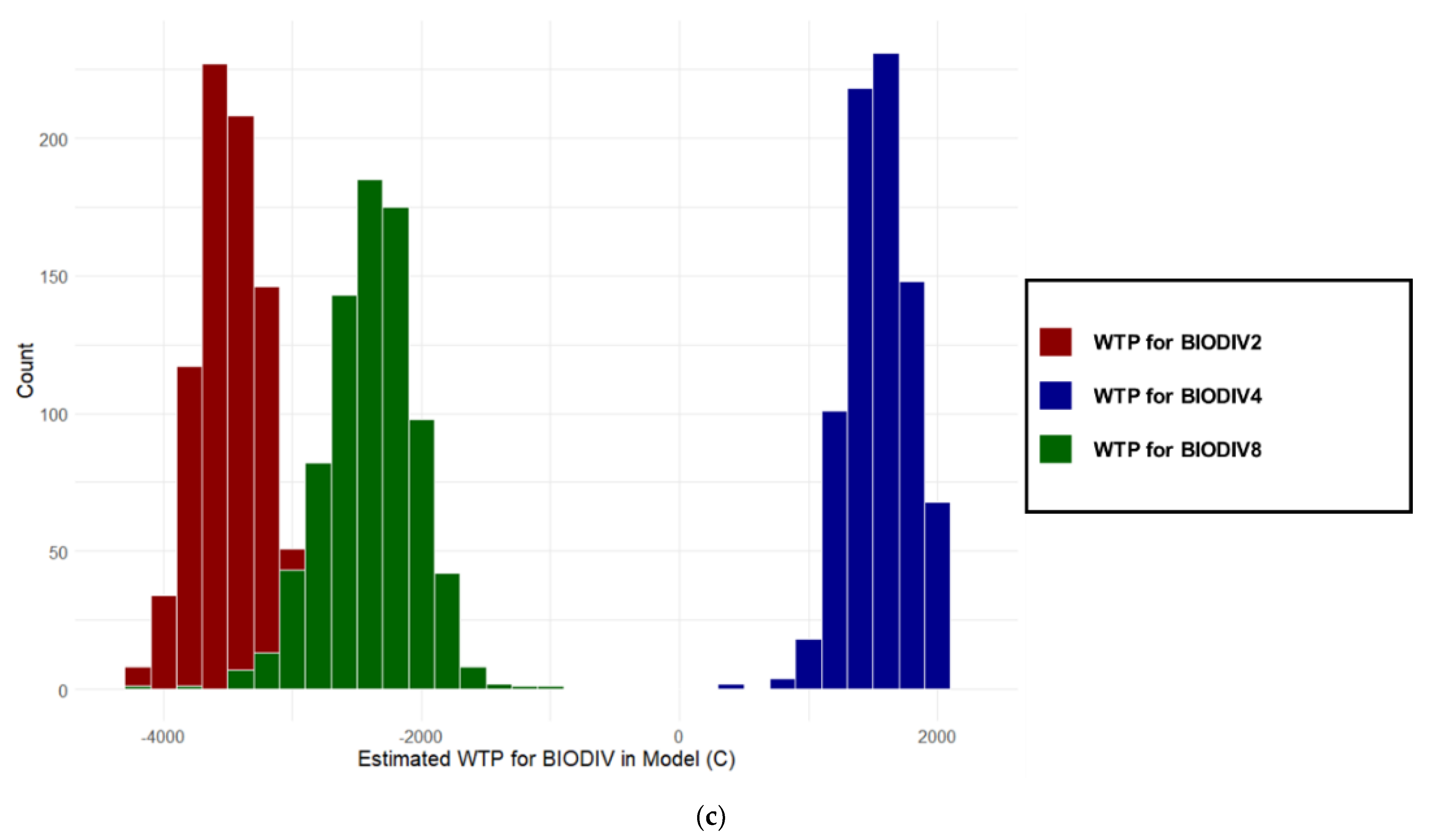
For the BIODIV variables, it is expected that all the variables will show a positive coefficient compared with the base variable (BIODIV0), and that BIODIV8 is the most preferred option, reflecting the positive value of biodiversity in the public. However, the results are opposite to the predictions; all the variables except for BIODIV4 show a negative mean coefficient and do not include zero. Additionally, the estimated WTP for BIODIV2 is smaller than that for BIODIV8 in Model (A), while the estimated WTP for BIODIV2 is larger than that for BIODIV8 in Models (B) and (C). Table 7 show that the estimated WTPs for BIODIV2 are JPY −1459, −2409, and −3483, and for BIODIV8, JPY −2681, −2020, and −2396 in Models (A), (B), and (C), respectively.

Finally, for LAMBDA, a positive coefficient is expected, which means that people’s preferences are positively spatially autocorrelated, based on previous studies [45,46,47,48]. Both spatial models show a positive LAMBDA coefficient. The LAMBDA coefficients are 0.535, and 0.275 for Models (B) and (C), respectively (see Table 6). Moreover, the estimated values for both models do not include zero. These results suggest that a positive spatial autocorrelation exists for people’s preferences, with the values varying slightly.

4. Discussion

4.1. Proximity to Agricultural Land and Satoyama as UGI

The estimation results reveal that people prefer agricultural land far away from their residence—more than 1000 m, rather than within 1000 m (see Table 6 and Table 7, and Figure 4, Figure 5 and Figure 6). This finding underscores the difficulty of using agricultural land as UGI in places close to residential areas and highlights that people dislike agricultural land in urban neighborhoods. This reflects the NIMBY phenomenon and has implications that are opposite to those of previous studies [42,43]. Modern agriculture in urban areas has positive and negative impacts on people, society, and the economy, as previous studies have discussed [6,19,20,21]. However, the results of this study suggest that the costs associated with the presence of agricultural land close to residential areas are deemed to exceed the corresponding benefits.

Given the above, policymakers and urban planners might consider providing and managing agricultural land as UGI in places far from residential areas to garner public support and improve the quality of people’s lives. Furthermore, it is recommended to take measures to alleviate the NIMBY phenomenon caused by concerns about traffic accidents and high criminality that are induced by poor visibility—for instance, by using security cameras, security lights, and visible traffic signs.

The results also reveal that people might prefer agricultural land approximately 200 m away from their residence than distances of 500 m and 1000 m (see Table 6 and Table 7, and Figure 4, Figure 5 and Figure 6). This result is contrary to the implication mentioned above and the NIMBY phenomenon. Within 1000 m from their residence, people prefer the indirect-use and non-use values of agricultural land (i.e., landscapes and cultural and educational value), e.g., [33,34]. It is difficult for people to receive these benefits from distant agricultural land (e.g., distance decay effect) [66]. People might demand value from an agricultural land if it exists within 1000 m from their residence. Therefore, it would be helpful for policymakers and urban planners to promote the land’s indirect-use and non-use values among people to alleviate the NIMBY phenomenon, such that the benefits of having agricultural land in the neighborhood exceed the associated costs.

4.2. Proximity to Satoyama as UGI

The estimation results show that people have different preferences regarding proximity to satoyama as UGI compared with agricultural land. People might prefer satoyama within 1000 m from their residence instead of a distance beyond 1000 m (see Table 6 and Table 7 and Figure 4, Figure 5 and Figure 6), which suggests that they might have received indirect-use value from neighboring satoyama, such as enjoyable sceneries. By contrast, people might not have benefitted from satoyama located beyond 1000 m from their residence. This result is in line with an earlier study [42,43].

In addition, for residences within 1000 m of satoyama or agricultural land, the negative impact of satoyama is larger than that of agricultural land. The differences of all the PROXSATO variables against the PROXSATO0 variables are larger than those of all the PROXAGRI variables against the PROXAGRI0 variables. This implies that people experience the costs associated with a neighboring satoyama to be higher than those from neighboring agricultural land, which reflects the complexity of satoyama land use.

The results highlight the difficulty of using satoyama close to residential areas as UGI and indicate that people prefer to travel to satoyama areas that are far away from their residence to consume ecological services. Due to the relatively large negative impacts, they do not want satoyama to be close to their residence. Therefore, policymakers and urban planners need to conserve satoyama land use in ways other than UGI, for instance, to collect entry fees for delivery of ecological services.

4.3. People’s Preference for Biodiversity

The results show that people do not prefer rich biodiversity around their neighborhood, as indicated by their preference regarding the number of species of dragonflies (see Table 6 and Table 7, and Figure 4, Figure 5 and Figure 6). The results indicate that the idea of biodiversity is also regarded negatively, similar to agricultural land and satoyama. In recent years, the importance of biodiversity has increased as the knowledge and contribution of biodiversity have been shared among people, and biodiversity conservation has received more attention and is being supported globally, also in Japan [35,55,56]. However, according to the results, people are not keen about rich biodiversity, at least around their housing.

Furthermore, the estimation results show that the WTP for BIODIV2 is smaller than that for BIODIV8. This result implies that people consider poor biodiversity to be worse than rich biodiversity. Therefore, from sharing knowledge about biodiversity, people may prefer rich biodiversity to poor biodiversity if their residence is distant from the environment that has richer biodiversity.

4.4. People’s Non-Linear Preference Regarding Proximity to AUGI

The results show the complexity of people’s preferences regarding proximity to AUGI, and this study choice experiment provides an opportunity to understand these preferences for agricultural land and satoyama. People’s proximity preferences show a nonlinear shape with the proximity. According to Glenk et al. (2020), both linear and non-linear shapes of proximity preferences for environmental goods and services are found in the literature [66]; meanwhile, this study finds that a non-linear shape might be more appropriate.

Moreover, the results indicate that complicated non-linear shapes might also be appropriate. In particular, people’s preferences could change greatly when the proximity is 0 m (neighboring) or 1000 m (far away). This result suggests that a more detailed investigation of people’s proximity preferences is needed.

4.5. Positive Spatial Autocorrelation in People’s Preferences

The estimation results reveal that a relatively strong positive spatial autocorrelation exists in people’s preferences. This indicates that there is a spatial concentration of residents with similar preference regarding the proximity of their residence to AUGI. This result is in line with previous research that finds positive spatial autocorrelation in people’s preferences for environmental goods and services [44,45,46,47]. The preference regarding the surrounding environment is one of the factors that influence resident’s decisions on where to locate his/her housing [67]. In other words, residents who share the surrounding environment may have similar preferences for the environment, forming local clusters. This phenomenon, called spatial sorting, may explain the positive spatial autocorrelation of people’s preferences regarding the proximity of their residence to AUGI, and if so, people’s housing choices may be the cause of the positive spatial autocorrelation of people’s preferences.

In addition, according to Figure 4, Figure 5 and Figure 6, more convergent results can be obtained by explicitly introducing spatial autocorrelation in the estimation models. This result emphasizes the importance of considering the spatial aspects when evaluating people’s preferences for environmental goods and services. Ignoring spatial autocorrelation in people’s preferences can lead to underestimation or overestimation of WTP, and this misspecification can mean misleading policy implications.

However, this study cannot address why positive spatial autocorrelation is observed in people’s preferences. This is a limitation of the study that should be explored in future research. In future work, two feasible hypotheses are suggested [67]. First, people decide where they reside according to their preferences for environmental goods and services, as mentioned above. In this case, the reason for positive spatial autocorrelation can be people’s residential choices. Second, people who reside in the same area are influenced by the same environmental goods, services, and the people around them. Such environmental and social interactions can make people’s preferences become similar.

4.6. Limitations and Future Research

This study has several limitations, and avenues for future research are hereby acknowledged. First, it is necessary to expand the study to generalize the results to other study areas, such as more urbanized areas. In the present study, the sample was collected from a residence in Ishikawa Prefecture in Japan, where people are expected to be familiar with agriculture, and some previous studies similarly collected their samples [35,36]. For more robust results, collecting samples from more urbanized areas, such as Tokyo, could be helpful.

Second, other evaluation methods, such as the hedonic price model, can be used in future work. The choice experiment was used in the present study to observe people’s choices for various residences. However, the hypothetical choice in the stated preference method can generate bias in the choices (e.g., hypothetical bias). Investigations using the hedonic price model and comparison of the results among different studies are necessary to obtain more robust results.

Third, as mentioned above, the cause of spatial autocorrelation in people’s preferences cannot be investigated. In future work, a causality analysis is necessary to explore the underlying causes of the spatial autocorrelation. Although some future work remains, our study has significantly contributed to studies on people’s preferences for environmental goods and services.

5. Conclusions

The present study investigated people’s preferences regarding the proximity of their residence to UGI, such as agricultural land and satoyama, as well as the possibilities of using agricultural land/satoyama as UGI. An online survey was administered to obtain spatially structured data from the choice experiment.

In summary, the hierarchical Bayes estimation of the random parameter logit model with spatial autocorrelation performed well and generated empirical evidence that supports the following findings. First, people’s preferences regarding proximity to agricultural land can be complicated. They prefer agricultural land far away from their residence—at more than 1000 m distance—not within 1000 m. This reflects the NIMBY phenomenon. Moreover, agricultural land as UGI in places with neighboring residential areas might require more attention than other UGI, and people prefer agricultural land approximately 200 m away from their residence instead of distances of 500 m or 1000 m. The preferred distance from agricultural land can be influenced by both the NIMBY phenomenon and the indirect-use value and non-use value of agricultural land.

Meanwhile, the results on people’s preferences regarding proximity to satoyama are complex. Specifically, they prefer satoyama within 1000 m instead of beyond 1000 m from their residence because of the indirect-use value of satoyama land. Moreover, people’s proximity preferences differ for satoyama versus agricultural land, and using satoyama as UGI in places with neighboring residential areas might be challenging.

Other findings were also obtained. People might not prefer rich (versus poor) biodiversity around their residence. This finding implies that the idea of biodiversity might also be subject to the NIMBY phenomenon, despite the biodiversity’s contributions to people. People’s preferences regarding proximity to environmental goods and services have a nonlinear shape with the proximity. It is statistically confirmed that there is positive spatial autocorrelation in people’s preferences.

Based on the results of this study, it is vital for policymakers and urban planners to manage and provide AUGI far from residential areas. Using AUGI in urban areas can reduce negative environmental impacts and develop sustainable urban areas [4,5,6,16]. To take advantage of AUGI with public supports, policymakers and urban planners may need to design residential areas and AUGI separately. In addition, as another practical option, it might be helpful to share the contributions of AUGI or prevent AUGI from having negative impacts to diminish people’s avoidance of neighboring AUGI.

AUGI should be further investigated for improving the quality of residents’ lives and for developing sustainable urban areas. Current urban areas have not contributed to environmental conservation; instead, they have had negative impacts [68,69]. Introducing AUGI is expected to help reduce such negative impacts on urban areas [21]. Therefore, it is necessary to evaluate urban people’s preferences for AUGI to incorporate such knowledge to the management of AUGI.

References

- Benedict, M.A.; McMahon, E.T. Green Infrastructure: Linking Landscapes and Communities; Island Press: Washington, DC, USA, 2012. [Google Scholar]
- European Commission. Communication from the Commission to the European Parliament, The Council, the European Economic and Social Committee and the Committee of the Regions. Green Infrastructure (GI)—Enhancing Europe’s Natural Capital; COM 2013, 249 Final; European Commission: Luxembourg, 2013. [Google Scholar]
- Pauleit, S.; Liu, L.; Ahern, J.; Kazmierczak, A. Multifunctional green infrastructure planning to promote ecological services in the city. In Urban Ecology. Patterns, Processes, and Applications; Niemela, J., Ed.; Oxford University Press: Oxford, UK, 2011; pp. 272–285. [Google Scholar]
- Hansen, R.; Pauleit, S. From multifunctionality to multiple ecosystem services? A conceptual framework for multifunctionality in green infrastructure planning for urban areas. Ambio 2014, 43, 516–529. [Google Scholar] [CrossRef] [PubMed] [Green Version]
- Van Oijstaeijen, W.; Van Passel, S.; Cools, J. Urban green infrastructure: A review on valuation toolkits from an urban planning perspective. J. Environ. Manag. 2020, 267, 110603. [Google Scholar] [CrossRef]
- Rolf, W.; Pauleit, S.; Wiggering, H. A stakeholder approach, door opener for farmland and multifunctionality in urban green infrastructure. Urban For. Urban Green. 2019, 40, 73–83. [Google Scholar] [CrossRef]
- Lafortezza, R.; Davies, C.; Sanesi, G.; Konijnendijk, C.C. Green Infrastructure as a tool to support spatial planning in European urban regions. iForest Biogeosciences For. 2013, 6, 102. [Google Scholar] [CrossRef] [Green Version]
- Mell, I.C. Green infrastructure: Reflections on past, present and future praxis. Landsc. Res. 2017, 42, 135–145. [Google Scholar] [CrossRef] [Green Version]
- Pauleit, S.; Hansen, R.; Rall, E.; Zölch, T.; Andersson, E.; Luz, A.; Szaraz, L.; Tosics, I.; Vierikko, K. Urban landscapes and green infrastructure. In Environmental Science. Oxford Research Encyclopedias; Shugart, H.H., Ed.; Oxford University Press: Oxford, UK, 2017; pp. 6–28. [Google Scholar]
- Muller, N.; Werner, P.; Kelcey, J.G. Urban Biodiversity and Design; Wiley-Blackwell: Chichester, UK, 2010. [Google Scholar]
- Andersson, E.; Barthel, S.; Borgström, S.; Colding, J.; Elmqvist, T.; Folke, C.; Gren, Å. Reconnecting cities to the biosphere: Stewardship of green infrastructure and urban ecosystem services. Ambio 2014, 43, 445–453. [Google Scholar] [CrossRef] [Green Version]
- Apreda, C.; Reder, A.; Mercogliano, P. Urban morphology parameterization for assessing the effects of housing blocks layouts on air temperature in the Euro-Mediterranean context. Energy Build. 2020, 223, 110171. [Google Scholar] [CrossRef]
- Reder, A.; Rianna, G.; Mercogliano, P.; Castellari, S. Parametric investigation of Urban Heat Island dynamics through TEB 1D model for a case study: Assessment of adaptation measures. Sustain. Cities Soc. 2018, 39, 662–673. [Google Scholar] [CrossRef]
- Bowler, D.E.; Buyung-Ali, L.; Knight, T.M.; Pullin, A.S. Urban greening to cool towns and cities: A systematic review of the empirical evidence. Landsc. Urban Plan. 2010, 97, 147–155. [Google Scholar] [CrossRef]
- Demuzere, M.; Orru, K.; Heidrich, O.; Olazabal, E.; Geneletti, D.; Orru, H.; Bhave, A.G.; Mittal, N.; Feliu, E.; Faehnle, M. Mitigating and adapting to climate change: Multi-functional and multi-scale assessment of green urban infrastructure. J. Environ. Manag. 2014, 146, 107–115. [Google Scholar] [CrossRef]
- Liu, W.; Chen, W.; Peng, C. Influences of setting sizes and combination of green infrastructures on community’s stormwater runoff reduction. Ecol. Model. 2015, 318, 236–244. [Google Scholar] [CrossRef]
- Tzoulas, K.; Korpela, K.; Venn, S.; Yli-Pelkonen, V.; Kaźmierczak, A.; Niemela, J.; James, P. Promoting ecosystem and human health in urban areas using Green Infrastructure: A literature review. Landsc. Urban Plan. 2007, 81, 167–178. [Google Scholar] [CrossRef] [Green Version]
- Madureira, H.; Nunes, F.; Oliveira, J.V.; Cormier, L.; Madureira, T. Urban residents’ beliefs concerning green space benefits in four cities in France and Portugal. Urban For. Urban Green. 2015, 14, 56–64. [Google Scholar] [CrossRef]
- Ackerman, K.; Conard, M.; Culligan, P.; Plunz, R.; Sutto, M.P.; Whittinghill, L. Sustainable food systems for future cities: The potential of urban agriculture. Econ. Soc. Rev. 2014, 45, 189–206. [Google Scholar]
- Dunn, A.D. Siting green infrastructure: Legal and policy solutions to alleviate urban poverty and promote healthy communities. BC Envtl. Aff. L. Rev. 2010, 37, 41. [Google Scholar]
- La Rosa, D.; Barbarossa, L.; Privitera, R.; Martinico, F. Agriculture and the city: A method for sustainable planning of new forms of agriculture in urban contexts. Land Use Policy 2014, 41, 290–303. [Google Scholar] [CrossRef]
- Rolf, W.; Peters, D.; Lenz, R.; Pauleit, S. Farmland—An Elephant in the Room of Urban Green Infrastructure? Lessons learned from connectivity analysis in three German cities. Ecol. Indic. 2018, 94, 151–163. [Google Scholar] [CrossRef]
- Ostoić, S.K.; van den Bosch, C.C.K.; Vuletić, D.; Stevanov, M.; Živojinović, I.; Mutabdžija-Bećirović, S.; Lazarević, J.; Stojanova, B.; Blagojević, D.; Stojanovska, M.; et al. Citizens’ perception of and satisfaction with urban forests and green space: Results from selected Southeast European cities. Urban For. Urban Green. 2017, 23, 93–103. [Google Scholar] [CrossRef]
- Wan, C.; Shen, G.Q. Salient attributes of urban green spaces in high density cities: The case of Hong Kong. Habitat Int. 2015, 49, 92–99. [Google Scholar] [CrossRef]
- Bergstrom, J.C.; Ready, R.C. What have we learned from over 20 years of farmland amenity valuation research in North America? Rev. Agric. Econ. 2009, 31, 21–49. [Google Scholar] [CrossRef]
- Gibbons, S.; Mourato, S.; Resende, G.M. The amenity value of English nature: A hedonic price approach. Environ. Resour. Econ. 2014, 57, 175–196. [Google Scholar] [CrossRef] [Green Version]
- Herath, S.; Choumert, J.; Maier, G. The value of the greenbelt in Vienna: A spatial hedonic analysis. Ann. Reg. Sci. 2015, 54, 349–374. [Google Scholar] [CrossRef] [Green Version]
- Hite, D.; Jauregui, A.; Sohngen, B.; Traxler, G. Open Space at the Rural-Urban Fringe: A Joint Spatial Hedonic Model of Developed and Undeveloped Land Values. 2006. Available online: http://ssrn.com/abstract=916964 (accessed on 19 June 2021).
- Hoshino, T.; Kuriyama, K. Measuring the benefits of neighbourhood park amenities: Application and comparison of spatial hedonic approaches. Environ. Resour. Econ. 2010, 45, 429–444. [Google Scholar] [CrossRef]
- Liu, T.; Hu, W.; Song, Y.; Zhang, A. Exploring spillover effects of ecological lands: A spatial multilevel hedonic price model of the housing market in Wuhan, China. Ecol. Econ. 2020, 170, 106568. [Google Scholar] [CrossRef]
- Melichar, J.; Kaprová, K. Revealing preferences of Prague’s homebuyers toward greenery amenities: The empirical evidence of distance–size effect. Landsc. Urban Plan. 2013, 109, 56–66. [Google Scholar] [CrossRef]
- Münch, A.; Nielsen, S.P.P.; Racz, V.J.; Hjalager, A.M. Towards multifunctionality of rural natural environments?—An economic valuation of the extended buffer zones along Danish rivers, streams and lakes. Land Use Policy 2016, 50, 1–16. [Google Scholar] [CrossRef]
- Ready, R.C.; Abdalla, C.W. The amenity and disamenity impacts of agriculture: Estimates from a hedonic pricing model. Am. J. Agric. Econ. 2005, 87, 314–326. [Google Scholar] [CrossRef]
- Walls, M.; Kousky, C.; Chu, Z. Is what you see what you get? The value of natural landscape views. Land Econ. 2015, 91, 1–19. [Google Scholar] [CrossRef]
- Shoyama, K.; Managi, S.; Yamagata, Y. Public preferences for biodiversity conservation and climate-change mitigation: A choice experiment using ecosystem services indicators. Land Use Policy 2013, 34, 282–293. [Google Scholar] [CrossRef]
- Duke, J.M.; Ilvento, T.W. A conjoint analysis of public preferences for agricultural land preservation. Agric. Resour. Econ. Rev. 2004, 33, 209–219. [Google Scholar] [CrossRef] [Green Version]
- Yang, X.; Burton, M.; Cai, Y.; Zhang, A. Exploring heterogeneous preference for farmland non-market values in Wuhan, Central China. Sustainability 2016, 8, 12. [Google Scholar] [CrossRef] [Green Version]
- Escobedo, F.J.; Kroeger, T.; Wagner, J.E. Urban forests and pollution mitigation: Analyzing ecosystem services and disservices. Environ. Pollut. 2011, 159, 2078–2087. [Google Scholar] [CrossRef] [PubMed]
- Lyytimäki, J.; Sipilä, M. Hopping on one leg–The challenge of ecosystem disservices for urban green management. Urban For. Urban Green. 2009, 8, 309–315. [Google Scholar] [CrossRef]
- Von Döhren, P.; Haase, D. Ecosystem disservices research: A review of the state of the art with a focus on cities. Ecol. Indic. 2015, 52, 490–497. [Google Scholar] [CrossRef]
- Dear, M. Understanding and overcoming the NIMBY syndrome. J. Am. Plan. Assoc. 1992, 58, 288–300. [Google Scholar] [CrossRef]
- Conedera, M.; Del Biaggio, A.; Seeland, K.; Moretti, M.; Home, R. Residents’ preferences and use of urban and peri-urban green spaces in a Swiss mountainous region of the Southern Alps. Urban For. Urban Green. 2015, 14, 139–147. [Google Scholar] [CrossRef]
- Sturm, R.; Cohen, D. Proximity to urban parks and mental health. J. Ment. Health Policy Econ. 2014, 17, 19. [Google Scholar]
- Campbell, D.; Scarpa, R.; Hutchinson, W.G. Assessing the spatial dependence of welfare estimates obtained from discrete choice experiments. Lett. Spat. Resour. Sci. 2008, 1, 117–126. [Google Scholar] [CrossRef]
- Chen, T.D.; Wang, Y.; Kockelman, K.M. Where are the electric vehicles? A spatial model for vehicle-choice count data. J. Transp. Geogr. 2015, 43, 181–188. [Google Scholar] [CrossRef] [Green Version]
- Czajkowski, M.; Budziński, W.; Campbell, D.; Giergiczny, M.; Hanley, N. Spatial heterogeneity of willingness to pay for forest management. Environ. Resour. Econ. 2017, 68, 705–727. [Google Scholar] [CrossRef] [Green Version]
- Morton, C.; Anable, J.; Yeboah, G.; Cottrill, C. The spatial pattern of demand in the early market for electric vehicles: Evidence from the United Kingdom. J. Transp. Geogr. 2018, 72, 119–130. [Google Scholar] [CrossRef] [Green Version]
- UNESCO. Oku-Noto no Aenokoto. Available online: https://en.unesco.org/silkroad/silk-road-themes/intangible-cultural-heritage/oku-noto-no-aenokoto (accessed on 17 June 2021).
- FAO. Noto’s Satoyama and Satoumi, Japan. Available online: http://www.fao.org/giahs/giahsaroundtheworld/designated-sites/asia-and-the-pacific/notos-satoyama-and-satoumi/detailed-information/en/ (accessed on 17 June 2021).
- Kadoya, T.; Washitani, I. The Satoyama Index: A biodiversity indicator for agricultural landscapes. Agric. Ecosyst. Environ. 2011, 140, 20–26. [Google Scholar] [CrossRef]
- Kobori, H.; Primack, R.B. Participatory conservation approaches for satoyama, the traditional forest and agricultural landscape of Japan. AMBIO J. Hum. Environ. 2003, 32, 307–311. [Google Scholar] [CrossRef]
- Louviere, J.J.; Hensher, D.A.; Swait, J.D. Stated Choice Methods: Analysis and Applications; Cambridge University Press: Cambridge, UK, 2000. [Google Scholar]
- Goertzen, D.; Suhling, F. Promoting dragonfly diversity in cities: Major determinants and implications for urban pond design. J. Insect Conserv. 2013, 17, 399–409. [Google Scholar] [CrossRef]
- Sahlén, G.; Ekestubbe, K. Identification of dragonflies (Odonata) as indicators of general species richness in boreal forest lakes. Biodivers. Conserv. 2001, 10, 673–690. [Google Scholar] [CrossRef]
- Nijkamp, P.; Vindigni, G.; Nunes, P.A. Economic valuation of biodiversity: A comparative study. Ecol. Econ. 2008, 67, 217–231. [Google Scholar] [CrossRef]
- Bakhtiari, F.; Jacobsen, J.B.; Strange, N.; Helles, F. Revealing lay people’s perceptions of forest biodiversity value components and their application in valuation method. Glob. Ecol. Conserv. 2014, 1, 27–42. [Google Scholar] [CrossRef] [Green Version]
- ChoiceMetrics. Ngene 1.2.0 User Manual & Reference Guide; ChoiceMetrics: Sydney, Australia, 2018. [Google Scholar]
- Train, K.E. Discrete Choice Methods with Simulation, 2nd ed.; Cambridge University Press: Cambridge, MA, USA, 2009. [Google Scholar]
- LeSage, J.; Pace, R.K. Introduction to Spatial Econometrics; Chapman and Hall/CRC: Boca Raton, FL, USA, 2009. [Google Scholar]
- Casella, G.; George, E.I. Explaining the Gibbs sampler. Am. Stat. 1992, 46, 167–174. [Google Scholar]
- Anselin, L. Under the hood issues in the specification and interpretation of spatial regression models. Agric. Econ. 2002, 27, 247–267. [Google Scholar] [CrossRef]
- Patuelli, R.; Arbia, G. (Eds.) Spatial Econometric Interaction Modelling; Springer: New York, NY, USA, 2016. [Google Scholar]
- Kostov, P. Model boosting for spatial weighting matrix selection in spatial lag models. Environ. Plan. B Plan. Des. 2010, 37, 533–549. [Google Scholar] [CrossRef] [Green Version]
- Kelejian, H.; Piras, G. Spatial Econometrics; Academic Press: London, UK, 2017. [Google Scholar]
- Stakhovych, S.; Bijmolt, T.H. Specification of spatial models: A simulation study on weights matrices. Pap. Reg. Sci. 2009, 88, 389–408. [Google Scholar] [CrossRef]
- Glenk, K.; Johnston, R.J.; Meyerhoff, J.; Sagebiel, J. Spatial dimensions of stated preference valuation in environmental and resource economics: Methods, trends and challenges. Environ. Res. Econ. 2020, 75, 215–242. [Google Scholar] [CrossRef]
- Toledo-Gallegos, V.M.; Long, J.; Campbell, D.; Börger, T.; Hanley, N. Spatial clustering of willingness to pay for ecosystem services. J. Agric. Econ. 2021. [Google Scholar] [CrossRef]
- Mori, K.; Christodoulou, A. Review of sustainability indices and indicators: Towards a new City Sustainability Index (CSI). Environ. Impact Assess. Rev. 2012, 32, 94–106. [Google Scholar] [CrossRef]
- Mori, K.; Yamashita, T. Methodological framework of sustainability assessment in City Sustainability Index (CSI): A concept of constraint and maximisation indicators. Habitat Int. 2015, 45, 10–14. [Google Scholar] [CrossRef]
Figure 1.
(a) Location of Ishikawa Prefecture in Japan. (b) Ishikawa Prefecture, Noto region and, Kaga region. Source: the author.
Figure 2.
The land use pattern of Ishikawa Prefecture. Source: made by the author based on National Land Numerical Information Land Use Fragmented Mesh Details.
Figure 3.
Spatial distribution of the respondents and the agricultural area. Note: the black dots indicate the respondents’ location. The respondents who reported the same parcel are shown by the same dot. Source: the author.
Figure 4.
Distribution of the estimated WTPs for Model (A). Note: (a) shows the distribution of the estimated WTP for the proximity to agricultural land derived from Model (A), (b) shows the distribution of the estimated WTPs for the proximity to satoyama and (c) shows the distribution of the estimated WTPs for the number of dragonflies around the residence.
Figure 5.
Distribution of the estimated WTPs for Model (B). Note: (a) shows the distribution of the estimated WTPs for the proximity to agricultural land derived from Model (A), (b) shows the distribution of the estimated WTPs for the proximity to satoyama and (c) shows the distribution of the estimated WTPs for the number of dragonflies around the residence.
Figure 6.
Distribution of the estimated WTPs for Model (C). Note: (a) shows the distribution of the estimated WTPs for the proximity to agricultural land derived from Model (A), (b) shows the distribution of the estimated WTPs for the proximity to satoyama and (c) shows the distribution of the estimated WTPs for the number of dragonflies around the residence.