Using Bidirectional Long Short-Term Memory Method for the Height of F2 Peak Forecasting from Ionosonde Measurements in the Australian Region

Abstract

The height of F2 peak (hmF2) is an essential ionospheric parameter and its variations can reflect both the earth magnetic and solar activities. Therefore, reliable prediction of hmF2 is important for the study of space, such as solar wind and extreme weather events. However, most current models are unable to forecast the variation of the ionosphere effectively since real-time measurements are required as model inputs. In this study, a new Australian regional hmF2 forecast model was developed by using ionosonde measurements and the bidirectional Long Short-Term Memory (bi-LSTM) method. The hmF2 value in the next hour can be predicted using the data from the past five hours at the same location. The inputs chosen from a location of interest include month of the year, local time (LT), $K_p$, $F_{10.7}$ and hmF2 as an independent variable vector. The independent variable vectors in the immediate past five hours are considered as an independent variable set, which is used as an input of the new Australian regional hmF2 forecast model developed for the prediction of hmF2 in the hour to come. The performance of the new model developed is evaluated by comparing with those from other popular models, such as the AMTB, Shubin, ANN and LSTM models. Results showed that: (1) the new model can substantially outperform all the other four models. (2) Compared to the LSTM model, the new model is proven to be more robust and rapidly convergent. The mew model also outperforms that of the ANN model by around 30%. (3) the minimum sample number for the bi-LSTM method (i.e., 2000) to converge is about 50% less than that is required for the LSTM method (i.e., 3000). (4) Compared to the Shubin model, the bi-LSTM method can effectively forecast the hmF2 values up to 5 h. This research is a first attempt at using the deep learning-based method for the application of the ionospheric prediction.

1. Introduction

The height of F2 peak (hmF2) is an essential ionospheric parameter that is defined by the altitude of electron density ($N_e$) peak in the ionosphere. The variation of the hmF2 reflects the ionospheric variability. Therefore, it can also reveal the activity of either the earth magnetic field (B) or the solar wind [1,2]. In addition, hmF2 forecasting can be considerably important in analysing the structure of ionosphere and enhancing both GNSS positioning and LEO orbit determination (especially during scintillation) capabilities.

The hmF2 can be obtained through a number of techniques, such as digisondes/ionosondes, GNSS radio occultation satellites and topside sounders. Ionosonde is a typical ionospheric sounding device that has been used widely for over 90 years (can be traced back to 1920s [3]) due to its high accuracy. Currently, there are hundreds of ionosonde stations operating all over the globe, and each station can provide hmF2 in 30 min frequency. Therefore, ionosonde-derived hmF2 has been widely used as the data source for ionosphere modelling (e.g., International Reference of Ionosphere (IRI) [4,5,6,7,8,9,10]). The ionosonde-only model developed by Altadill et al. [8]. is called the “AMTB” model which represents the first character of the four authors’ surnames. Concurrently, Hoque and Jakowski [11] established their model based on data from both the ionosonde measurements and radio occultation (RO), including Challenging Mini-satellite Payload (CHAMP), Gravity Recovery and Climate Experiment (GRACE), and Constellation Observing System for Meteorology, Ionosphere, and Climate (COSMIC). Shubin et al. [12] developed a hmF2 model based on radio occultation data from COSMIC, GRACE, and CHAMP only. The AMTB and Shubin’s models have been selected for the inclusion in the 2016 version (the latest version) of the IRI model [10].

Sai and Tulasi [13] carried out the hmF2 modelling in a different way. Most current models are established using known base functions (i.e., empirical orthogonal functions or spherical harmonics functions) which may not be perfect. Sai used the artificial neural network (ANN) technique, a machine learning method, to estimate the coefficients without knowing the base function of independent variables in advance from COSMIC (ibid). Tulasi [14] then further enhanced his model by including other RO measurements (i.e., GRACE and CHAMP) as well as ionosonde data as data sources. Furthermore, he also assessed the performance of the ANN model by comparing with IRI-2016 model, and also proved that the anomalies of ionosphere (e.g., equatorial ionosphere anomaly (EIA) and mid-latitude summer night-time anomaly (MSNA)) are well captured by the model [13,14].

All the above models, however, have a common disadvantage that several physical parameters, such as $F_{10.7}$ (a measure of solar flux per unit at a wavelength of 10.7 cm) and $K_p$ (a global geomagnetic activity index) which can only be measured in real time (or near-real time) are required as inputs for the hmF2 models. Therefore, the values of those physical parameters have to be estimated during the process of hmF2 forecasting which may impact the quality of the hmF2 output from the model.

In this study, a more advanced machine learning technique—bidirectional Long Short-Term Memory network (hereinafter termed “bi-LSTM”[15]) is used for predicting/forecasting hmF2 from ionosonde-only data at 12 ionosonde stations in the Australia region. In comparison with ANN, the bi-LSTM method can be considered as a special type of the recurrent neural network (RNN) technique which takes into account of the sequential variation of hmF2 value. This advantage offers us an opportunity to perform the prediction by using the data in recent epochs. However, this technique has some disadvantages. The most important one is that, the sample data of the model must be continuous (each sample set must have the same time intervals) and at the same location, which is not as flexible as ANN. This is another reason why the ionosonde data were selected for this study (i.e., continuous measurements at a fixed location). First, hmF2 models for each station were established and assessed, then a regional hmF2 model was built by considering the geographic location of the stations (i.e., longitude and latitude). The three models aforementioned, i.e., AMTB, Shubin and ANN models [16] were selected for comparison. The traditional LSTM model was used for the evaluation to show the advantages of the bi-LSTM. Out-of-sample ionosonde data were used as the reference.

The outline of the paper is as follows. Section 2 briefly introduces the measurements used and the variable set selected. Section 3 illustrates the fundamentals of the bi-LSTM method and the procedure of its usages to establish new hmF2 models with the variable set proposed. Section 4 presents various experiments conducted and the performance of the new model developed is assessed by comparing with the AMTB, Shubin, ANN and LSTM models. Conclusions are given in Section 5.

2. Data Sources

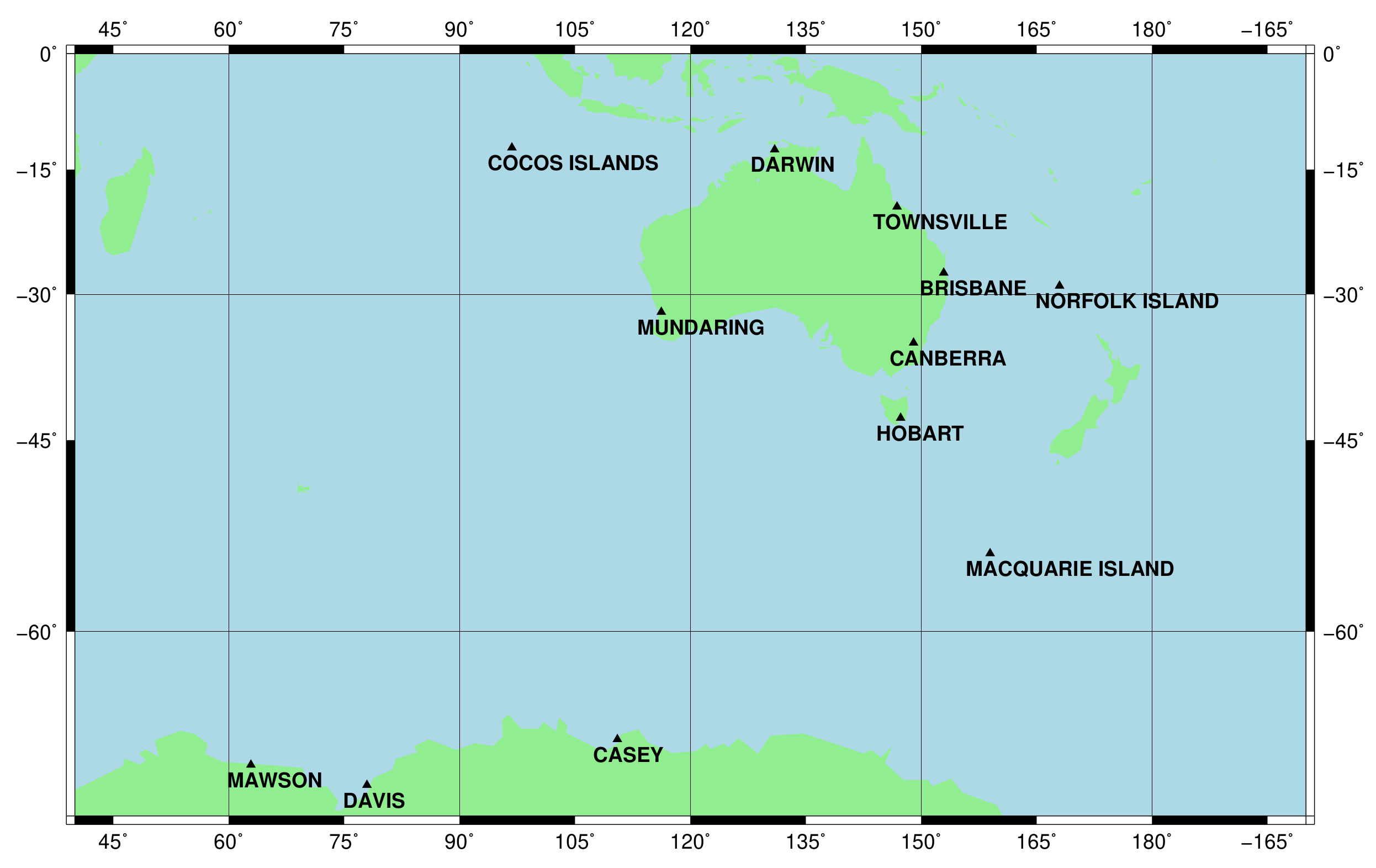
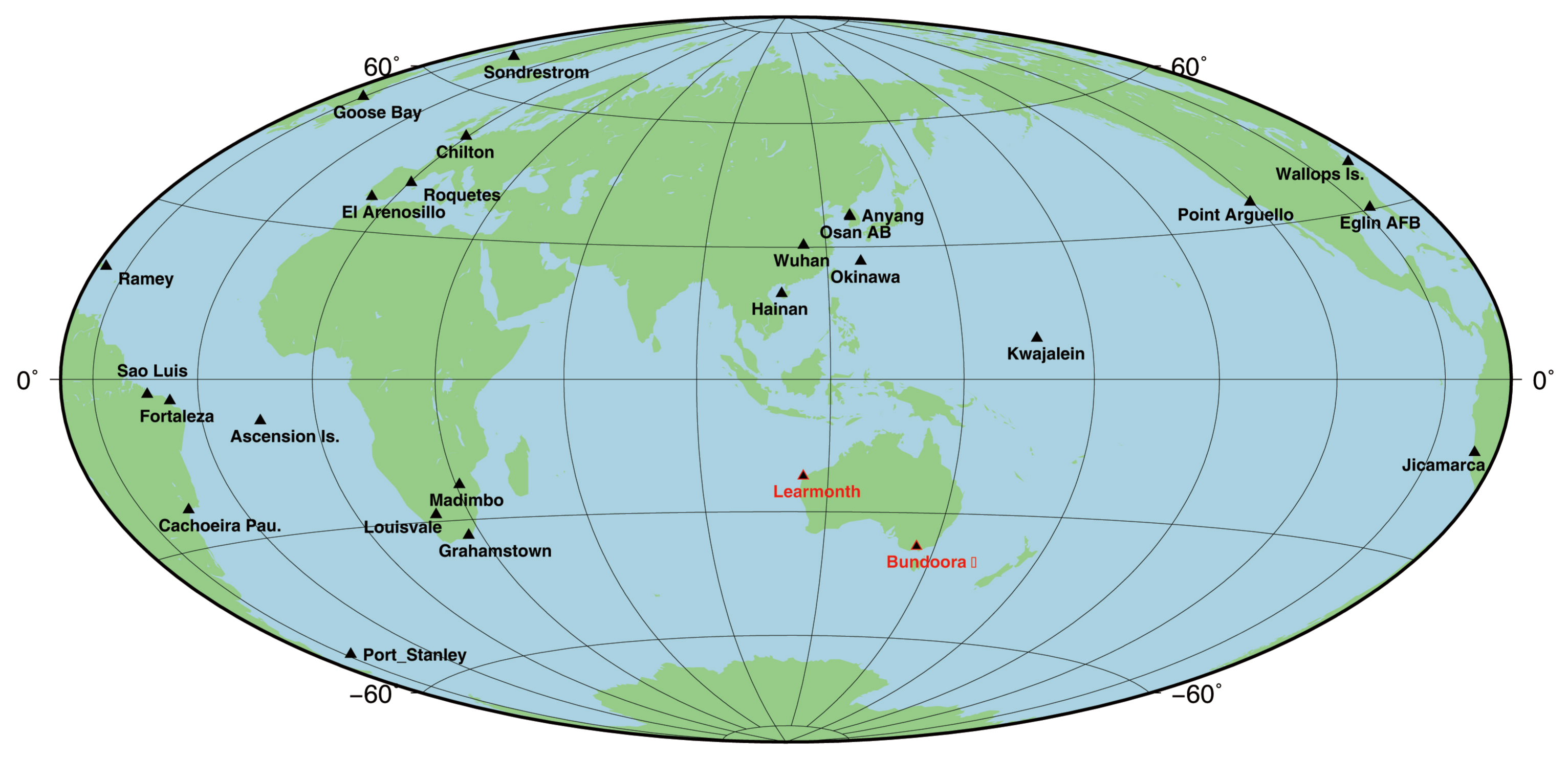
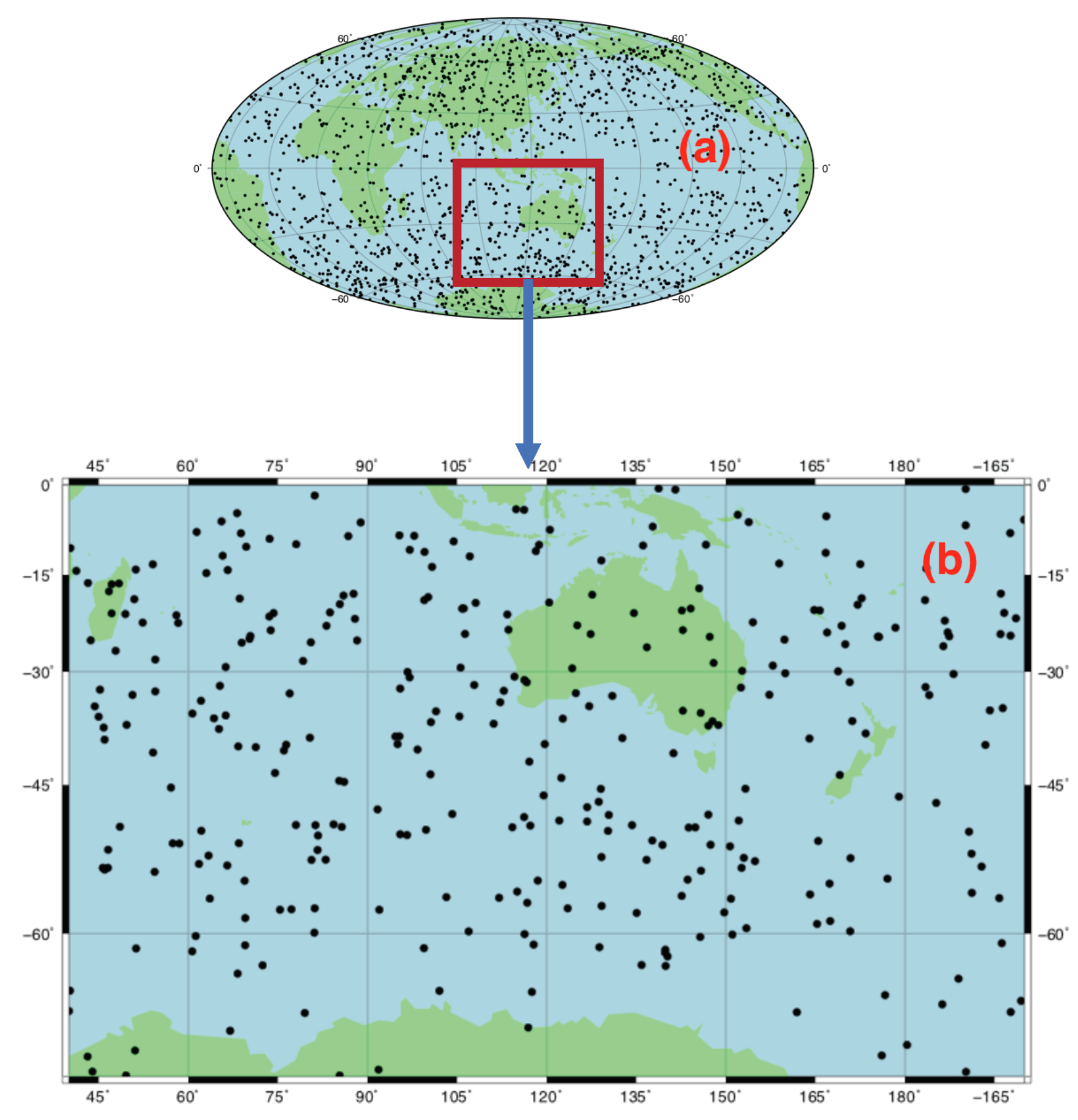
2.1. Ionosonde Stations

The ionosonde instrument was prototyped in 1925 and further enhanced in the late 1920s. An ionosonde typically consists of four parts: a high frequency (HF) radio transmitter; a HF receiver; an antenna with a suitable radiation pattern; and a central control and data processing system. There are more than 100 ionosonde stations deployed around the world that routinely measure the structure and variability of bottomside ionosphere using the reflection of radio waves (echo sounding) [17]. hmF2 is the peak altitude of the detection range. There are 12 ionosonde stations in Australia region (see Figure 1). The geographic location and operational period of these stations are detailed in

Table 1. Australian ionosonde stations and their geographic coordinates.

Station Name (Acronym)	Latitude	Longitude	Open	Closed
Cocos Islands (CI)	−12.20	96.80	Nov 1961	Sep 1974
			Aug 2008
Darwin (DW)	−12.45	130.95	Dec 1982
Townsville (TS)	−19.63	146.85	Jun 1946
Brisbane (BB)	−27.53	152.92	Jun 1943	Dec 1986
			Jun 1997
Norfolk Island (NI)	−29.03	167.97	Feb 1964
Mundaring (MD)	−31.98	116.22	Apr 1959	Dec 2007
Canberra (CB)	−35.32	149.00	Mar 1937
Hobart (HB)	−42.92	147.32	Dec 1945
Macquarie Islands (MI)	−54.50	158.95	Jun 1950	Nov 1958
			Nov 1983	Jun 2015
Casey (CA)	−66.30	110.50	Jul 1957	Jan 1975
			Apr 1989	Mar 1992
			Nov 2000
Mawson (MS)	−67.60	62.88	Feb 1958
Davis (DA)	−68.58	77.96	Feb 1985

which suggests that they can provide enough samples for the proposed modelling work. In order to obtain stable quiet-time hmF2, monthly median hmF2 for each local hour were derived by using Equations (1)–(5) from various ionosonde measurements. The measurements are provided (manually scaled) by the Australian Bureau of Meteorology, which can be downloaded from ftp://ftp-out.sws.bom.gov.au/wdc/iondata/medians/) was selected as the samples, similar to the work did by Altadill et al. [8].

2.2. Variables

Month of the year, Local Time (LT), $K_p$, $F_{10.7}$, geographic longitude (only used for regional model), latitude (only used for regional model) and hmF2 at one epoch (hourly here) are considered as an independent variable vector. In this study, the variable vectors in five continuous hours at the same station are manually selected to form an independent variable set, and hmF2 in the 6th (i.e., next hour) is considered to be dependent on the variable set.

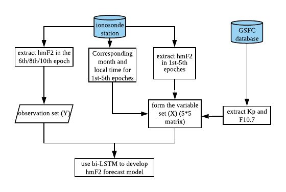
3. Methodology

3.1. hmF2 Generation

Three kinds of measurements from ionosonde data are required for the calculation of hmF2: (1) $F_2$ peak plasma frequency ($foF2$); (2) the ratio of the maximum usable frequency at a distance of 3000 km to the $foF2$ (M(3000)F2); and (3) E peak plasma frequency (foE) [18]. The equations are:

$${\varphi }_1=(2.32·{10}^{-3})·R_{12}+0.222$$

(1)

$${\varphi }_2=1.2-(1.16·{10}^{-2})·exp[(2.39·{10}^{-2})·R_{12}]$$

(2)

$${\varphi }_3=0.096·(R_{12}-25)/150$$

(3)

$$\Delta M=\frac{{\varphi }_1·(1.0-\frac{R_{12}}{150}·exp[-\frac{{\lambda }^2}{1600}])}{r-{\varphi }_2}+{\varphi }_3$$

(4)

$$hmF2=1490.0/\left[M3000\right(F2)+\Delta M]-176$$

(5)

where $R_{12}$ reflects the strength of solar activity (that can be obtained from https://omniweb.gsfc.nasa.gov/cgi/nx1.cgi), $\lambda$ is the magnetic dip latitude (that can be obtained from the IGRF-12 model). ${\varphi }_{1,2,3}$ and $\Delta M$ are the temporal values during hmF2 calculation, and $r=foF2/foE$. These equations are also currently used in the IRI model.

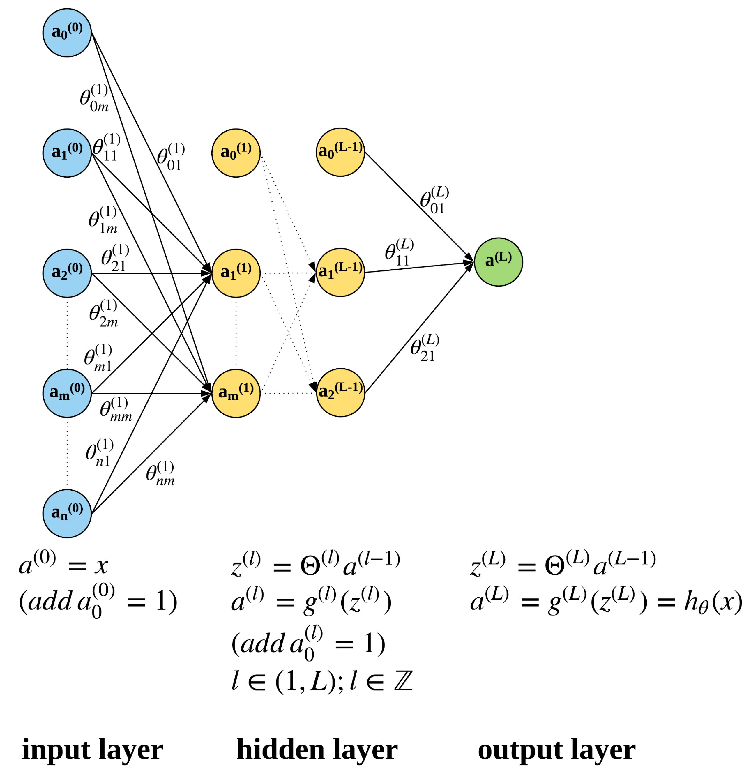
3.2. Artificial Neural Network (ANN)

The detailed structure of an ANN system is shown in Figure 2 where a three-layer structure is used. From left to right are: input, hidden and output layers respectively. It should be noted that more than one sublayer can exist in the hidden layer. The equations in the figure describe how forward propagation works (i.e., the second step in the neural network procedure). The superscript of a denotes the index of the layer and the subscript of a denotes the index of the cell in the current layer. ${\mathsf{\Theta }}^{\left(f\right)}$ is the cluster of all $\theta$ in the lth layer, and ${\theta }_{nb}^{\left(l\right)}$ is for transmitting the cell n in the $(l-1)$th layer to cell b in the lth layer. In addition, ‘$a_0^l$’s in Figure 2 denote the bias unit (equal to 1) in each layer, and l is the index of the layer. During the backward propagation (in this study, the mini-batch gradient descent [19,20] is selected as the backward approach), $\mathsf{\Theta }$ will be optimized together with the cost function. x and $h_{\theta }\left(x\right)$ are the input and output of the model respectively. In addition, $g^{\left(l\right)}$ is the activation function for the lth layer, which is normally highly non-linear, such as ReLU, tanh and sigmoid. Their equations are expressed as follows:

$$ReLU\left(x\right)=max(0,x)$$

(6)

$$tanh\left(x\right)=\frac{e^x+e^{-x}}{e^x-e^{-x}}$$

(7)

$$Sigmoid\left(x\right)=\frac{1}{1+e^{-x}}$$

(8)

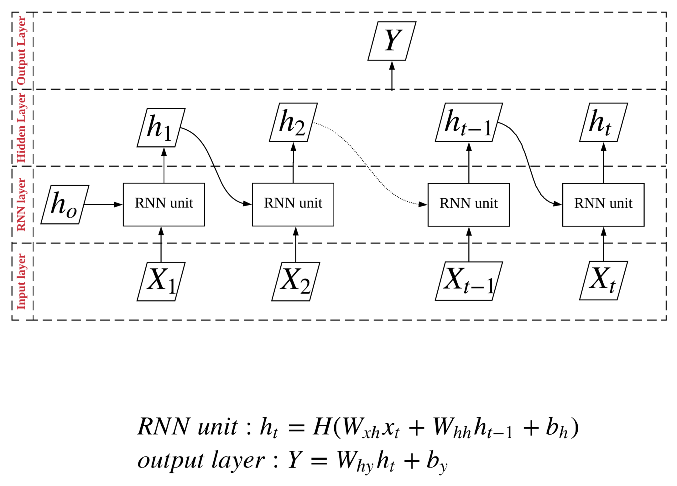
3.3. Recurrent Neural Network (RNN)

RNN takes sequential variation among sample data into consideration which is ignored by the ANN method. The structure of an RNN system is detailed in Figure 3. In comparison with the ANN, temporary results from the current epoch will influence the model in the next epoch. $X_t$ is the independent variable set at the tth epoch, and Y is the independent variable. $h_t$ is the temporary results from the tth RNN unit, $h_0$ is manually initialised. The connection between h and Y are normal SoftMax/regression. Each RNN unit can be considered as an ANN model (Figure 2). Ws and bs are the coefficients and biases needed to be estimated during training. In addition, H is the $tanh$ function.

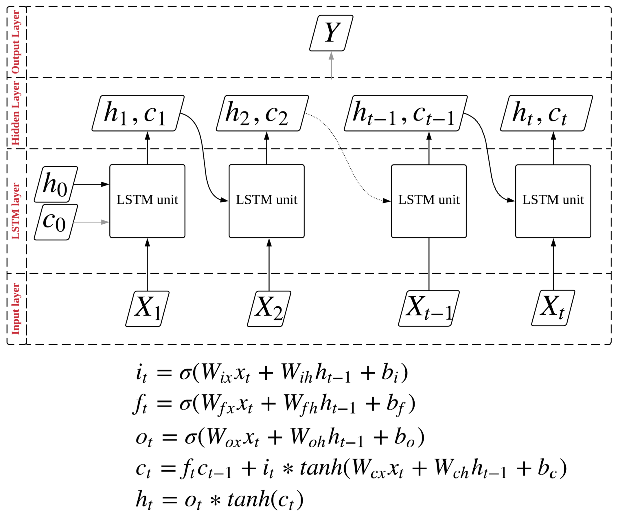
3.3.1. Long Short-Term Memory (LSTM) Method

Currently, LSTM method is one of the most widely used RNN methods which inherits the advantages of RNN. In addition, the influence of sample data at a specific epoch to the traditional RNN unit will dwindle with the epoch going by. In order to investigate the feature of the temporal sequences, a new type of interim result—memory cell c is applied in LSTM as is shown in Figure 4. c can keep the historical data in memory, and wake it up in any epoch when needed. The Input gate (i) and Forget gate (f) decide the relative weights of this RNN cell and historical memory cell respectively, and o is output gate. The detail algorithm is described in Figure 4 as well.

3.3.2. Bidirectional LSTM (bi-LSTM) Method

Memory cells in LSTM can carry forward the information from previous sample sets into the prediction of Y ultimately. However, the implementation process is directional, forward-only, which ignores the backward connection and makes the model less robust. To solve this disadvantage, the training process in the bi-LSTM method is conducted in a sequential order not only forward, but also backward. The details of the bi-LSTM method are shown in Figure 5.

In this study, the components of X are:

$$X_t^s=(mont{h}_t,L{T}_t,K{p}_t,F{10.7}_t,{hmF2}_t)$$

(9)

$$X_t^r=(mont{h}_t,L{T}_t,K{p}_t,lo{n}_t,la{t}_t,F{10.7}_t,{hmF2}_t)$$

(10)

$X_t^s$ (from Equation (9)) and $X_t^r$ (from Equation (10)) are independent variable sets for stationary and regional models respectively. t in Figure 5 equals to 5, thereby $Y=hmF{2}_{t+1}$.

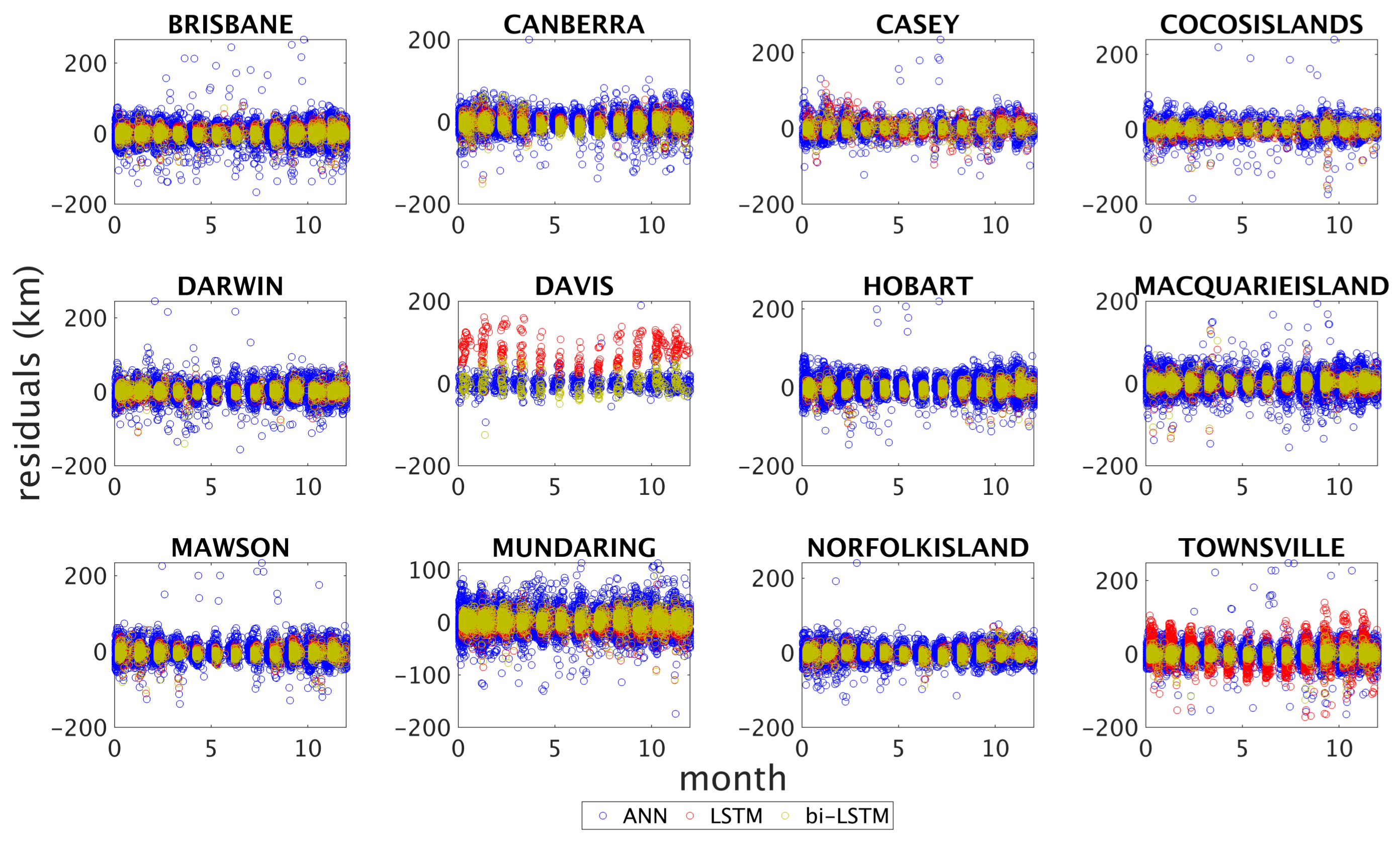
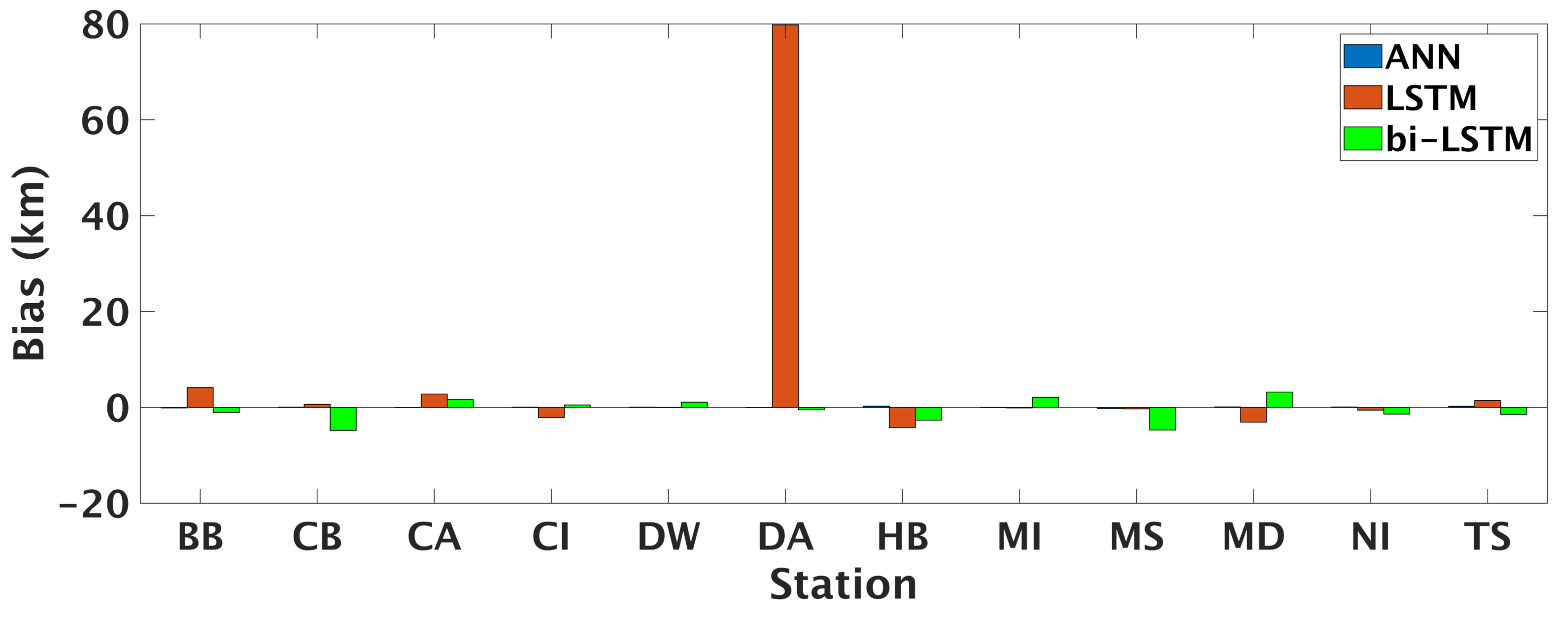
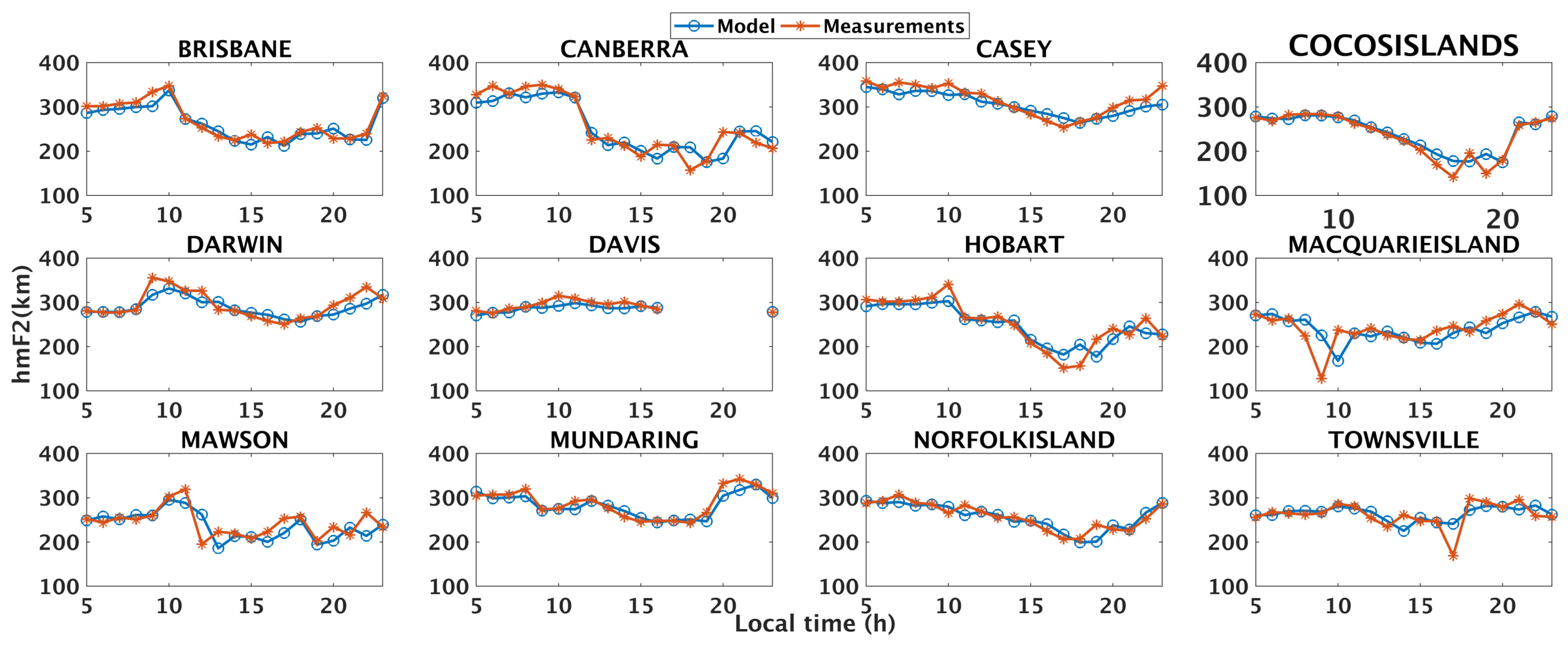
4. Results

In this study, only the stations that have more than 1000 sample sets (data in each station are detailed in Figure 6b) are selected (the aforementioned 12 Australian ionosonde stations, whose data can be downloaded from ftp://ftp-out.sws.bom.gov.au/wdc/iondata/). Three latest models (i.e., AMTB, Shubin and ANN models), together with the LSTM model are used for various comparisons and 10% out-of-sample datasets are selected as the reference. First two models can be obtained using IRI-2016, and for Tulasi’s method, the same ANN configuration is used to reproduce the model from ionosonde data. As shown in Equation (11), the Root Mean Squares (RMS) value is used to assess the performance of the models.

$$RMS=\sqrt{\frac{{\sum }_{i=1}^n{({\widehat{x}}_i-x_i)}^2}{n}}$$

(11)

where n is the number of testing data, $\widehat{x}$ and x are the measured and predicted $hmF2$ values respectively. Before the start of the modelling, a number of LSTM configurations have been tested (not shown here), and L2 regularised factor with the ADAM method is proven to be the optimal choice for both LSTM and bi-LSTM in this study.

As is shown in Figure 6a, the performance of different models using sample sets from different ionosonde stations is investigated and the numbers of sample sets are plotted in Figure 6b. Both two figures are sorted by the number of sample sets in an ascending order. Figure 6 reveals that the models from the LSTM and the bi-LSTM methods outperform the other three models in all stations except the DAVIS station where only 1000 sample sets are available. DAVIS as a typical example station is discarded in this study due to its limited number of observations. The hmF2 performance at the three discarded stations is shown in Figure 7 and it is clear that both LSTM and bi-LSTM models produce large RMSEs. The LSTM and bi-LSTM models converge at 3000 sample sets at the CI station and 2000 sample sets at the CASEY station respectively. Hence, it is estimated that the minimum sample number to converge is around 2000 for the bi-LSTM method and 3000 for the LSTM method respectively. Moreover, an abrupt increase of RMSE happens in the TOWNSVILLE station when the LSTM method is used. It shows that the bi-LSTM method is more robust than the LSTM method since the bi-LSTM curve presents a smooth nature.

The models for predicting more than one hour were also developed and analysed. Figure 8 presents the performance of three models using the bi-LSTM for predicting hmF2 in 1, 3 and 5 h forward at each station (hereinafter called ‘bi-LSTM-1h’, ‘bi-LSTM-3h’, ‘bi-LSTM-5h’ respectively). The Shubin model is also included as a reference. Figure 8 shows that the performance of the bi-LSTM model degenerates with the increase of the time (hours) forecast forward. The performance of the bi-LSTM-5h is slightly worse than that of Shubin model under the current configuration. Finding a better configuration (even the optimal configuration) of bi-LSTM model to make bi-LSTM available in further forward forecasting will be our next focus towards on this direction.

It is interesting to note that the performance of the AMTB model (based on ionosonde data) is worse than Shubin’s model (based on COSMIC data) with reference to the Australian ionosonde data since the same type of data was used in the AMTB model. The geographic distribution of the data used for producing both AMTB and Shubin’s models is investigated to further study this phenomenon. The ionosonde stations selected for AMTB model are plotted in Figure 9, which indicates that only two stations (shown in red) are available in the Australian region (i.e., Learmonth and Bundoora). Figure 10a shows the global distribution of all RO events measured on 1 January 2009, and Figure 10b is the RO events in the Australian region. Compared to Figure 9, the number of RO events is much more densely and homogeneously distributed in the Australian region than that of the ionosonde stations. This may explain that why Shubin’s model is much closer to the reference in this study than the AMTB model.

The variation of the residuals in relation to the time at each of the 12 stations is plotted in Figure 11 based on different modelling approaches (i.e., ANN, LSTM and bi-LSTM). The LSTM residuals are predominantly around 0 (without any systematic bias) except those at the DAVIS station (see Figure 12). This finding further echoes our previous conclusion that 1000 sample sets are not enough for the LSTM method to converge. It is also found that the bi-LSTM method can converge with fewer sample sets compared to that of the LSTM method. At TOWNSVILLE, the systematic bias is low, but random discrepancies are high, which implies that the LSTM method (compared to the bi-LSTM method) could not capture the characteristics of the sequential variations of hmF2 at TOWNSVILLE well using a 5-h sample set. Therefore, a longer sample set may be required for the training of this station’s model values in future.

The Australian regional models were established using ANN, LSTM and bi-LSTM based on the ionosonde sample sets from all ionosonde stations. Their RMSs listed in

Table 2. RMS of different Australian regional models.

	RMS (km)
ANN	22.1
LSTM	15.64
bi-LSTM	15.42

show that with enough sample sets, the performance of the LSTM and the bi-LSTM methods is similar (bi-LSTM is slightly better), and both can outperform ANN substantially (around 30%). Additionally, If the ANN model were used to generate hmF2 at one epoch, it would require $K_p$ and $F_{10.7}$ at that epoch as the inputs, but it is not required by the LSTM or bi-LSTM model. Its performance could be much worse if the estimated values were to be used during the prediction.

Figure 13 shows a comparison between the results from the Australian regional model and actual measurements at each station for a full day in January. Blue cycles and red asteroids in panels denote the model prediction and measurements respectively. Although there are no samples during 17-22 LT in DAVIS’s panel due to the lack of data from the station, the rest of the samples from DAVIS fit the model predictions well. In addition, an interesting anomaly is observed in Figure 13 that the variations of the model results are similar to those measurements but with one-hour delay (e.g., during 17-23 LT at CANBERRA; 9-11 LT at MACQUARIE ISLAND; and 10-18 LT at MANSON, etc). It may be caused by the influence from the sudden solar wind or cosmic radiation which cannot be captured by Kp (3-h time resolution). Hence, in future, we would like to take solar wind parameters (such as Interplanetary Magnetic Field) into consideration as independent variables to see if this anomaly can be mitigated.

5. Summary and Conclusions

In this study, a new Australian regional hmF2 forecast model was developed from ionosonde data using the bi-LSTM method. With this new model, hmF2 values can be predicted well forward up to five hours using the data in the past five hours. Month of the year, LT, geographic longitude and latitude, together with $K_p$, $F_{10.7}$ and hmF2, in the past five hours, were chosen as an independent variable set to model the hmF2 in the hour forward. Various assessments have been conducted by comparing the new model with the AMTB, Shubin, ANN and LSTM models. Results showed:

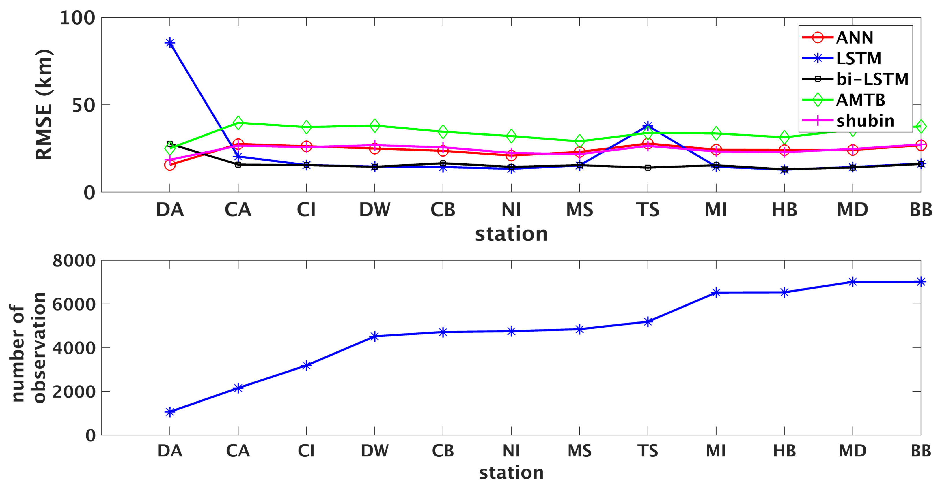
• The new bi-LSTM and LSTM models substantially outperform the other three tested models, even when real-time data are used as part of the input for these three models.
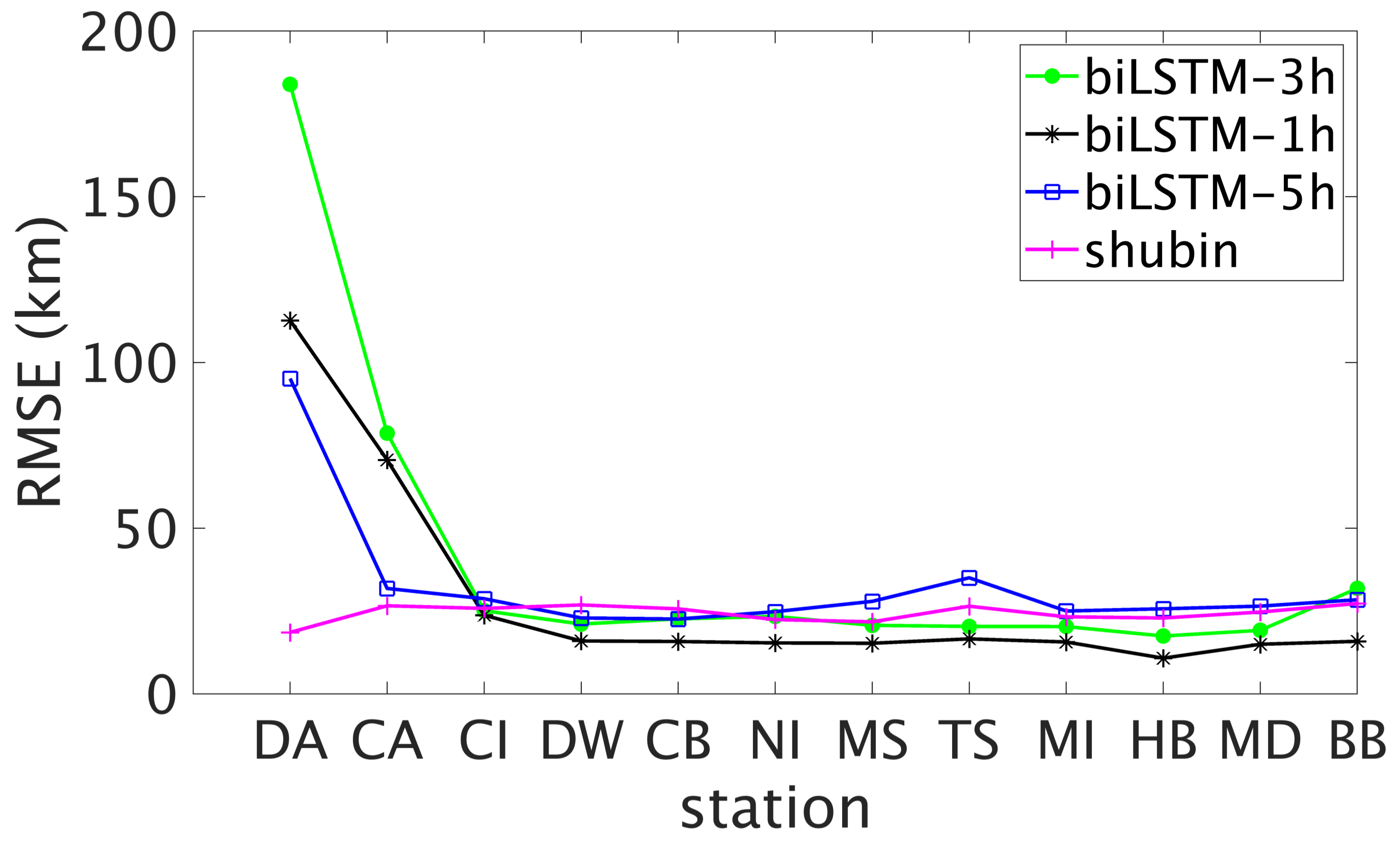
• The new model is more robust, and more easily and rapidly converge compared to the LSTM model. The overall performance improvement of the new bi-LSTM model is 30% compared to the ANN regional model.
• The minimum sample numbers for the LSTM and bi-LSTM methods to converge are around 3000 and 2000 respectively.
• The bi-LSTM-1h and bi-LSTM-3h (mentioned in Section 4, shown in Figure 8) agree better with ionosonde measurements compared to the Shubin model, but the bi-LSTM-5h is slightly worse than that of the Shubin model.
• The performance of the Shubin model is better than that of AMTB model in the Australian region.

This is our first attempt in predicting ionospheric parameter using deep learning approaches and it seems the neural network method is effective. However, significant further research is expected in future. In addition to the investigation of the independent variable set, the model can be also extended to a global model by using ionosonde data all over the world.

References

- Ngwira, C.M.; McKinnell, L.A.; Cilliers, P.J.; Coster, A.J. Ionospheric observations during the geomagnetic storm events on 24–27 July 2004: Long-duration positive storm effects. J. Geophys. Res. Space Phys. 2012, 117. [Google Scholar] [CrossRef]
- Goncharenko, L.; Salah, J.; Van Eyken, A.; Howells, V.; Thayer, J.; Taran, V.; Shpynev, B.; Zhou, Q.; Chau, J. Observations of the April 2002 geomagnetic storm by the global network of incoherent scatter radars. Ann. Geophys. 2005, 23, 163–181. [Google Scholar] [CrossRef] [Green Version]
- Davies, K. Ionospheric Radio; Number 31; IET: Stevanage, UK, 1990. [Google Scholar]
- Bilitza, D.; Hoegy, W. Solar activity variation of ionospheric plasma temperatures. Adv. Space Res. 1990, 10, 81–90. [Google Scholar] [CrossRef]
- Bilitza, D.; Huang, X.; Reinisch, B.W.; Benson, R.F.; Hills, H.K.; Schar, W.B. Topside ionogram scaler with true height algorithm (TOPIST): Automated processing of ISIS topside ionograms. Radio Sci. 2004, 39. [Google Scholar] [CrossRef]
- Bilitza, D.; Reinisch, B.W. International reference ionosphere 2007: Improvements and new parameters. Adv. Space Res. 2008, 42, 599–609. [Google Scholar] [CrossRef]
- Magdaleno, S.; Altadill, D.; Herraiz, M.; Blanch, E.; de La Morena, B. Ionospheric peak height behavior for low, middle and high latitudes: A potential empirical model for quiet conditions—Comparison with the IRI-2007 model. J. Atmos. Sol. Terr. Phys. 2011, 73, 1810–1817. [Google Scholar] [CrossRef]
- Altadill, D.; Magdaleno, S.; Torta, J.; Blanch, E. Global empirical models of the density peak height and of the equivalent scale height for quiet conditions. Adv. Space Res. 2013, 52, 1756–1769. [Google Scholar] [CrossRef]
- Bilitza, D.; Altadill, D.; Zhang, Y.; Mertens, C.; Truhlik, V.; Richards, P.; McKinnell, L.A.; Reinisch, B. The international reference ionosphere 2012—A model of international collaboration. J. Space Weather Space Clim. 2014, 4, A07. [Google Scholar] [CrossRef]
- Bilitza, D.; Altadill, D.; Truhlik, V.; Shubin, V.; Galkin, I.; Reinisch, B.; Huang, X. International reference ionosphere 2016: From ionospheric climate to real-time weather predictions. Space Weather 2017, 15, 418–429. [Google Scholar] [CrossRef]
- Hoque, M.; Jakowski, N. A new global model for the ionospheric F2 peak height for radio wave propagation. Ann. Geophys. Copernicus GmbH 2012, 30, 797. [Google Scholar] [CrossRef] [Green Version]
- Shubin, V.; Karpachev, A.; Tsybulya, K. Global model of the F2 layer peak height for low solar activity based on GPS radio-occultation data. J. Atmos. Sol. Terr. Phys. 2013, 104, 106–115. [Google Scholar] [CrossRef]
- Sai Gowtam, V.; Tulasi Ram, S. An artificial neural network-based ionospheric model to predict NmF2 and hmF2 using long-term data set of FORMOSAT-3/COSMIC radio occultation observations: Preliminary results. J. Geophys. Res. Space Phys. 2017, 122, 743–755. [Google Scholar] [CrossRef]
- Tulasi Ram, S.; Sai Gowtam, V.; Mitra, A.; Reinisch, B. The improved two-dimensional artificial neural network-based ionospheric model (ANNIM). J. Geophys. Res. Space Phys. 2018, 123, 5807–5820. [Google Scholar] [CrossRef]
- Schuster, M.; Paliwal, K.K. Bidirectional recurrent neural networks. IEEE Trans. Signal Process. 1997, 45, 2673–2681. [Google Scholar] [CrossRef] [Green Version]
- Schalkoff, R.J. Artificial Neural Networks; McGraw-Hill: New York, NY, USA, 1997; Volume 1. [Google Scholar]
- Prolss, G.W.; Bird, M.K. Physics of the Earth’s Space Environment: An Introduction; Springer: Berlin, Germany, 2004. [Google Scholar]
- Bilitza, D.; Eyfrig, R.; Sheikh, N. A global model for the height of the F2-peak using M3000 values from the CCIR numerical map. ITU Telecommun. J. 1979, 46, 549–553. [Google Scholar]
- Hinton, G.; Srivastava, N.; Swersky, K. Neural networks for machine learning lecture 6a overview of mini-batch gradient descent. Neural Netw. Mach. Learn. 2012, 14, 14. [Google Scholar]
- Ruder, S. An overview of gradient descent optimization algorithms. arXiv, 2016; arXiv:1609.04747. [Google Scholar]