A Microwave Tomography Strategy for Underwater Imaging via Ground Penetrating Radar
by
 , , , and
Giovanni Ludeno
1,* ,
,
Luigi Capozzoli
2,
Enzo Rizzo
2 ,
,
Francesco Soldovieri
1 and
Ilaria Catapano
1 1
Institute for Electromagnetic Sensing of the Environment, National Research Council of Italy, I-80124 Napoli, Italy
2
Institute of Methodologies for Environmental Analysis, National Research Council of Italy, I-85050 Tito (PZ), Italy
*
Author to whom correspondence should be addressed.
Remote Sens. 2018, 10(9), 1410; https://0-doi-org.brum.beds.ac.uk/10.3390/rs10091410
Submission received: 30 July 2018
/
Revised: 31 August 2018
/
Accepted: 4 September 2018
/
Published: 5 September 2018
(This article belongs to the Special Issue Recent Progress in Ground Penetrating Radar Remote Sensing)
Abstract
:Detection and monitoring of underwater structures is one of the most challenging applicative scenarios for remote sensing diagnostic techniques, among which ground penetrating radar (GPR). With this aim, an imaging strategy belonging to the family of microwave tomographic approaches is proposed herein. This strategy allows the imaging of objects located into a wet sand medium below a freshwater layer and it can find application in investigation of lakes, rivers, and hydraulic structures. The proposed strategy accounts for the layered structure of the scenario under test by exploiting a spatially variable equivalent permittivity in the inverse scattering model. This allows a reliable reconstruction of depth and horizontal size of underwater hidden objects. The imaging capabilities of the strategy are verified by processing experimental data referred to a laboratory environment reproducing a submerged archeological site at scale 1:1. The results are compared with those obtained by modelling the reference scenario as a homogeneous medium, in order to verify the effective improvement in terms of reconstruction accuracy.
1. Introduction
Ground penetrating radar (GPR) is a well-assessed imaging technology that allows subsurface analysis of the investigated area. This technique is non-invasive and non-destructive, utilizes low-power, and can perform surveys at different working frequencies (ranging from some tens of MHz to few GHz) depending on the adopted antenna system [1,2]. Moreover, thanks to its flexibility, GPR can be used in situ [3,4,5,6,7,8,9,10] or mounted on helicopters or drones [11,12,13,14,15].
Nowadays, GPR is widely employed in several applicative contexts. Examples are geological prospections [16], snow and ice characterization [12,17,18], assessment of the conservation state of valuable buildings from historical, archaeological, and structural points of view [3,9,10,19], inspection of road layers, railway, bridges or viaducts [7,8], and mapping of steel in reinforced concrete structures [6,20,21].
Additionally, another challenging applicative context is represented by the survey of underwater environments. Detection and imaging of underwater objects represent open issues for non-invasive sensing techniques and are among the relevant topics in the frame of the study of the effects of climate changes on cultural heritage assets. Indeed, the progressive temperature increase and the consequent extreme weather events involve a rise both of river water flow and sea level. In the first case, the rivers during the centuries carried a large percentage of organic material, such as wooden tools, fishing nets, remains of buildings, and so on, which are deposited on the bottom and create the so-called cultural layers [22]. On the other hand, the rise of the sea level is one of the main causes of the changes of the coastal lines occurred during the centuries, which caused the disappearance below the water level of ancient urban environments, like for instance the harbors of Roman Empire [23].
With respect to the survey of the underwater environments, microwaves are worth being considered, because they are able to survey beyond the water-bottom interface, allowing us to overcome the limits of conventional methods, mainly sonar instrumentations, which are suitable to retrieve the information related to the depth of the water bottom but not to detect the targets located below it. In this regard, GPR was capable of detecting hidden dangers at water bottoms such as cracking, uneven settlement, or uplifting [24].
On the other hand, GPR images do not provide an easily interpretable representation of the investigated scenario. Therefore, GPR effectiveness is often affected by the difficult interpretation of the raw data, which may be a very hard task and requires expert users. As a consequence, there is a constant effort toward the design and adoption of data-processing strategies capable of providing easily interpretable images [1,9,25,26,27,28]. In this context, microwave tomographic approaches, which face the imaging as the solution of an inverse scattering problem [29], have been proposed and their reconstruction capabilities have been verified by processing both synthetic and experimental data [10,12,14,30].
As a further contribution concerning the use of GPR for detection and localization of underwater targets, this manuscript aims at assessing the imaging capabilities offered by a microwave tomographic approach properly designed for the application at hand. This approach is able to provide reliable results without increasing the complexity of the mathematical formulation and while keeping low the computational cost. Moreover it, is based on an approximate scattering model capable of accounting for the layered structure of the reference scenario, which is made by a freshwater layer and a second medium of wet sand where the targets are buried. In particular, the scattering model adopted to perform the imaging is based on the following key features:
- (i)
- adoption of the Born approximation, which permits to formulate the imaging as a linear inverse problem;
- (ii)
- assumption that the materials are non-magnetic and lossless, specifically the material dispersive behavior is neglected in order to exploit frequency diversity of data;
- (iii)
- use of a two dimensional and ray-based model (by considering that the transmitting/receiving antennas are far, in terms of probing wavelength, from the water bottom) to express in a simple way the incident field and the Green’s function, which are the key elements of the mathematical relationship between data and unknown of the problem at hand; and
- (iv)
- introduction of an equivalent relative dielectric permittivity, from now on simply referred as equivalent permittivity, whose value depends on the distance of the antenna from the water-medium interface and the depth of the generic point into the investigation domain.
The introduction of the equivalent permittivity to describe the electromagnetic features of the reference scenario allows us to define the Green’s function and the incident field as for a homogeneous medium, while saving the possibility to obtain a reliable estimation of the target location and size. Accordingly, it avoids the necessity to consider a non-homogeneous reference scenario, which implies an increase of the mathematical complexity of the scattering model, i.e., of the data-unknown relationship (see [31] for details).
The concept of equivalent permittivity has been proposed previously in the frame of air-borne GPR imaging and tested on synthetic data [30]. In [30], the signal propagation occurs into a half space reference scenario, where the upper medium is air and the lower one is a medium such as ice, ground, sand, rock, and so on. In addition, the height of the antenna from the air-medium interface is a priori known. Conversely, in this manuscript, since the exact distance from the antenna to the water bottom is unknown, the profile of the freshwater-wet sand interface and its depth are preliminarily estimated from the data.
In order to verify the improvement in term of reconstruction capabilities offered by the proposed imaging approach, this manuscript deals with the analysis of radargrams referred to surveys performed on a scenario simulating a submerged archeological site. Specifically, the radargrams herein processed were collected at the Hydrogeosite Laboratory of CNR-IMAA, a concrete pool whose volume (about 230 m3) was partially filled with homogeneous silica sand and freshwater in order to simulate lacustrine and wet sand conditions. Furthermore, archaeological ruins of Roman times have been reproduced in the silica sand medium [32]. It is worth pointing out that all materials involved into experimental setup are characterized by a certain value of dielectric permittivity and a non-null conductivity.
Raw radar data were gathered by means of a GPR SIR3000 (GSSI Instruments, Nashua, NH, USA) equipped with antennas with carrier frequency equal to 400 MHz.
Results provided by the herein proposed approach are compared with those obtained by assuming that the signal propagation occurs into a homogeneous reference scenario.
2. Data Processing Approach
This section deals with the description of the scattering model used for the data processing and summarizes the adopted imaging approach, which involves two main steps: pre-processing and data inversion.
2.1. Pre-Processing
The pre-processing aims at extracting the useful signal from the raw data. Specifically, this step consists of several filtering procedures performed in time domain, which allow us to reduce noise and to remove the direct antenna coupling thus emphasizing the scattered field due to the target. Specifically, the time domain data processing begins with the zero-time correction and involves procedures such as time gating (TG) and background removal (BKR). Herein, these time domain procedures will be described briefly, more details can be found in [1,12,14,33].
The zero-timing consists in setting the zero-time of the B-scan, which is fixed in correspondence of the first signal peak, i.e., in correspondence of the time instant at which the receiving antenna begins to collect the backscattered field.
The TG procedure forces to zero the portion of the radargram corresponding to the antenna direct coupling or, more in general, the radargram portion that is outside the time window where the signal due to the targets of interest is expected.
The BKR consists in replacing the current radar trace, referred as A-scan, with the difference between it and the average value of all the A-scans as computed along the measurement axis. This operation erases all the flat interfaces present in the data (including the air-freshwater interface, only partially erased by the zero-timing) and usually provides a cleaner image of the buried scenario.
2.2. Data Inversion
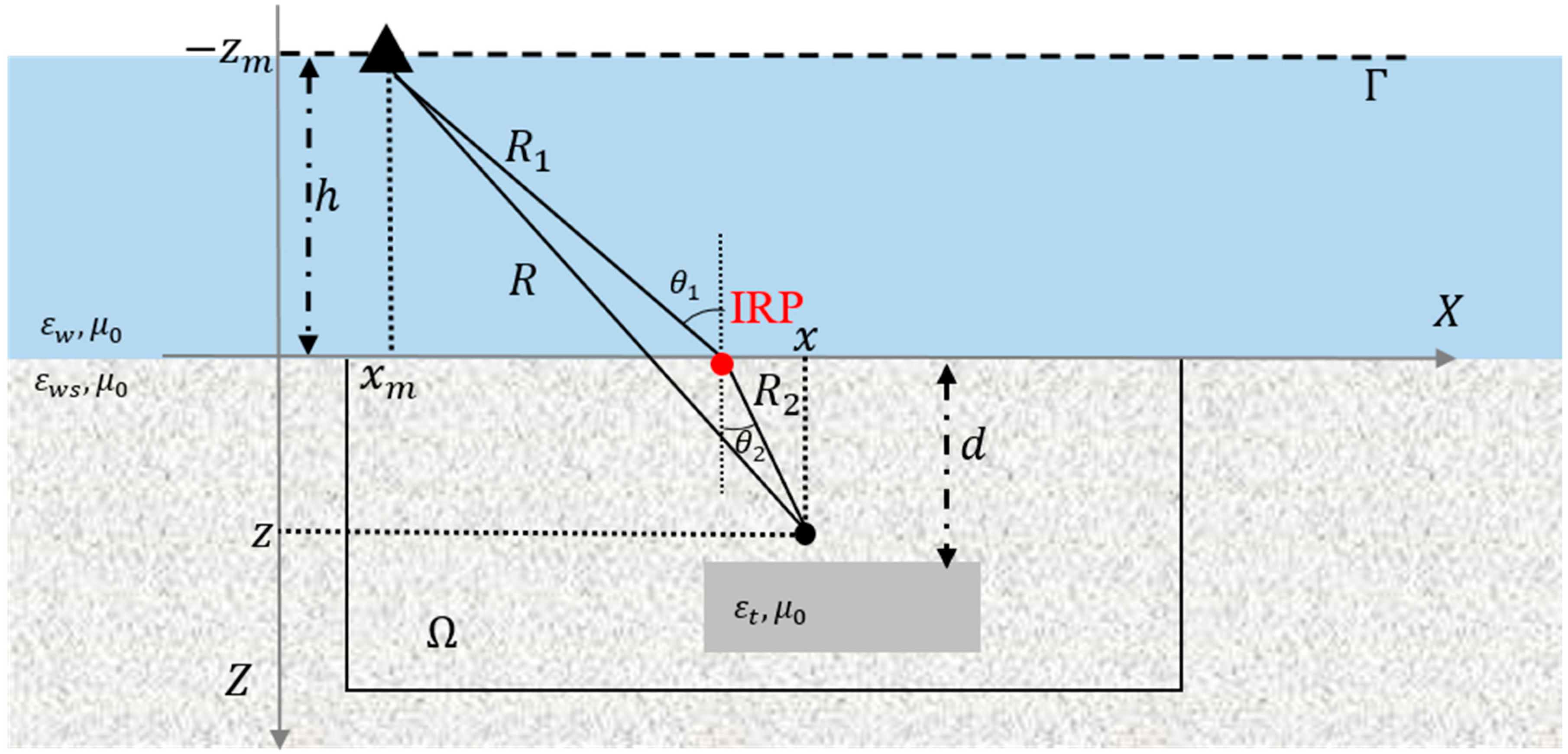
Let us consider the reference scenario in Figure 1. The signal propagation occurs in two media defined as freshwater and wet sand, which are characterized by dielectric permittivity values denoted as and , respectively. GPR antennas are located close to the freshwater surface at height h from the freshwater-wet sand interface and the target is at depth d in the wet sand medium.
The antennas are moved at a several measurement points , with m = 1, …, M, along a line , hence a multimonistatic measurement configuration is considered. Target is located into the investigated domain within the wet sand. The transmitting antenna is considered as a filamentary line source and the targets are modelled as cylinders of arbitrary cross-section, i.e., they are invariant along Y-axis and have an arbitrary shape into the X-Z plane. Therefore, the scattering phenomenon is formulated by accounting for the 2D scalar case. The targets, whose unknown dielectric permittivity is denoted by , are looked for as electromagnetic anomalies with respect to a reference scenario having relative dielectric permittivity .
Accordingly, the imaging approach considers as unknown the contrast function , which represents the difference between the permittivity of the targets and that of the surveyed medium, i.e., the permittivity of the reference scenario. The contrast is retrieved by the available multimonistatic multifrequency data by solving an inverse scattering problem, which is formulated in the frequency domain.
In order to simplify the mathematical model describing the relationship between the scattering electric field and the contrast function, the following hypothesis are made:
- The wave-material interaction is described according to the Born approximation, thus, the imaging is faced as a linear inverse scattering problem [34];
- The dispersive behavior of the materials involved in the scattering phenomenon is neglected and hence the contrast function does not change with the frequency;
- The transmitting and receiving antennas are considered in far-field zone with respect to the investigated area in terms of the probing wavelength;
- The targets are supposed to be far from the freshwater-wet sand interface in terms of the underground probing wavelength; and
- The propagation is described by means of an equivalent wave number , where is the wavenumber in air [30].
Accordingly, the linear equation to be solved is given as:
In Equation (1), the equivalent wavenumber is defined by the following equation:
where and denote the refractive index of the freshwater and wet sand, respectively, while the quantities and identify the path of the electromagnetic rays in freshwater and wet sand, with respect to the reflection point referred as the interface reflection point (IRP) (see Figure 1). The evaluation of the IRP is the most computationally challenging step of the method and entails, for each measurement point on and each generic point into , the solution of a non-linear equation, which is derived by exploiting the Snell’s law [12,35]. Finally, represents the Euclidean distance between the measurement point on and the generic point in .
In order to avoid the computation of the IRP and achieve a significant improvement in term of computational time, is assumed equal to one obtained along the ray path that is normal to the freshwater-wet sand interface [30]. According to this assumption, Equation (2) can be rewritten as:
which leads to:
This expression states that, based on the above hypothesis, the scattering phenomenon can be described by assuming that the propagation occurs in a medium whose wavenumber is spatially variable into the domain Ω (depending on z-coordinate of the generic point of Ω) and depends on the height h of the measurement line Γ from the freshwater bottom as well as on the relative refractive index of the host medium.
As it is shown in the next Sections, the inversion of the Equation (1) permits obtaining an accurate estimate of the geometrical features of the target, i.e., its location and size, while keeping low the computational burden. Of course, the inversion requires the knowledge of the height h, which may be estimated from the data as described in Section 3.2.
According to the strategy, already presented in other papers [10,12,14,29], Equation (1) is discretized by using the method of moments (MoM), where the contrast function is discretized in pixels and the imaging problem is formulated as the inversion of the resulting matrix L, as reported in the following equation:
This issue is addressed by using a regularization scheme based on the truncated singular value decomposition (TSVD) of L, in order to counteract the ill-conditioning of the discrete inverse problem, as described in [12].
It is worth noting, that the imaging result is given as the spatial 2D map of the modulus of the retrieved contrast function as normalized to its maximum value into the investigated domain. Hence, the regions of Ω where the modulus of the contrast are significantly different from zero indicate the targets.
3. GPR Surveys and Results
3.1. Experimental Test Site and Instrumentation Description
To understand the contribution that GPR can give to discover anthropic structures placed in water saturated soils, an extensive experimental activity was carried out at the Hydrogeosite Laboratory (Research Infrastructure of CNR-IMAA) in a reinforced concrete pool of size 12 m × 7 m × 2.7 m. Thanks to the facilities of this laboratory, it was possible to reproduce real scale case studies in laboratory conditions. Specifically, the pool was partially filled with homogeneous silica sand and freshwater in order to simulate lacustrine and wet sand conditions. Table 1 reports the chemical and hydrogeological parameters of the sand used for the experiment.
The freshwater has a relative dielectric permittivity equal to and electric conductivity , while the wet sand has relative dielectric permittivity equal to and electric conductivity whose value changes from about , according to the water content. The presence of 17 piezometers allows the control of the water table depth by making possible the simulation of scenarios characterized by the presence of sand with a different water content.
In a small area of the pool, several structures simulating archaeological targets were placed at different depths (Figure 2). Two main phases of research activity were performed. In the first one, several scenarios were reproduced with an increasing of the water content to study the influence of the water on the geophysical response [32]. In the second phase, a real underwater scenario was simulated, where the soil surface was placed of a distance of 0.30 m approximately from the air/water interface [36].
This paper presents results referred to the second phase, i.e., when the structures are completely submerged. The target of the research was addressed to realize an archaeological context that is often found in Italy near rivers or lakes.
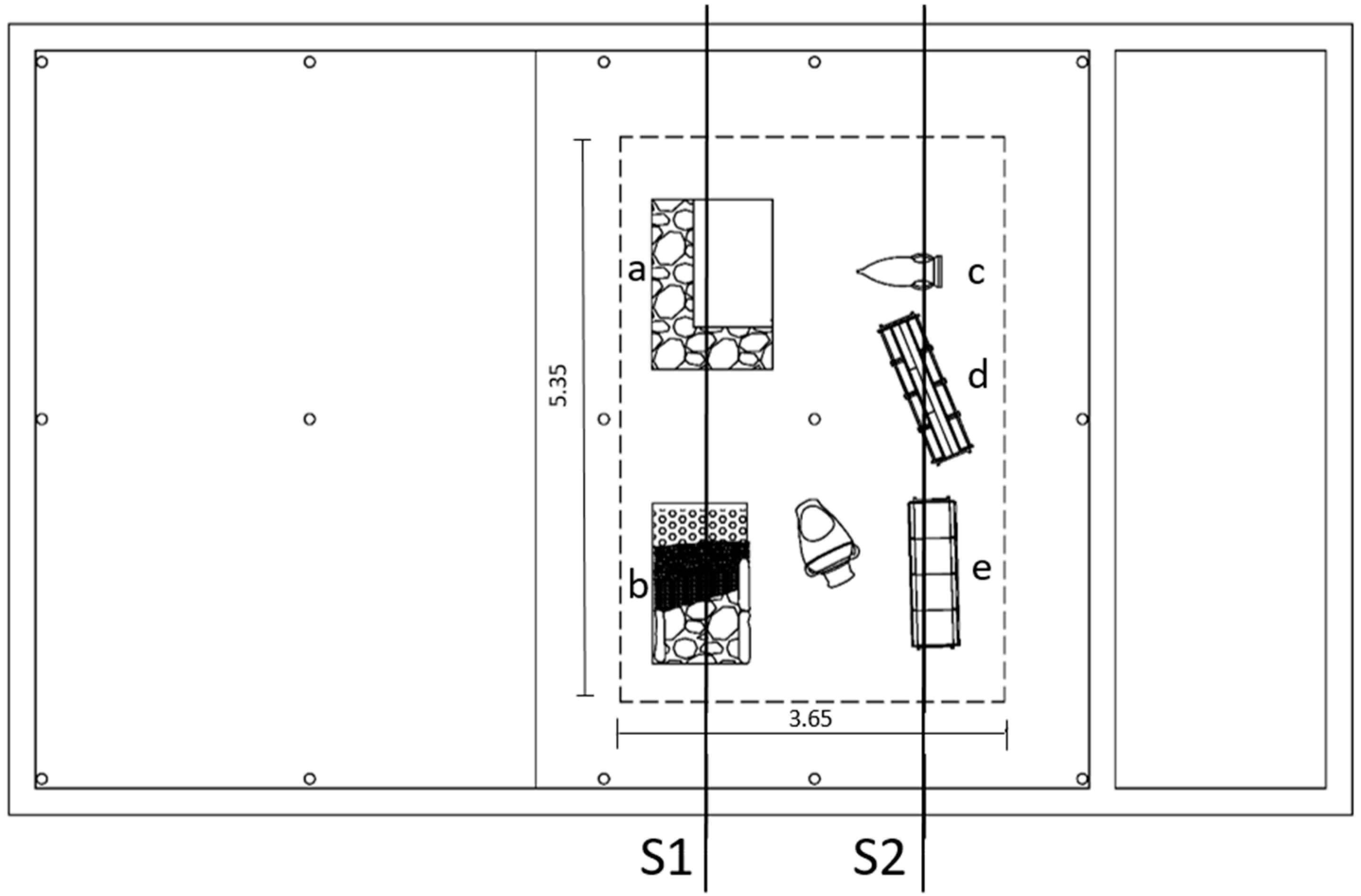
It is worth pointing out that all the structures are aligned along two lines, referred to as S1 and S2 and corresponding to the two GPR profiles here processed (see Figure 2).
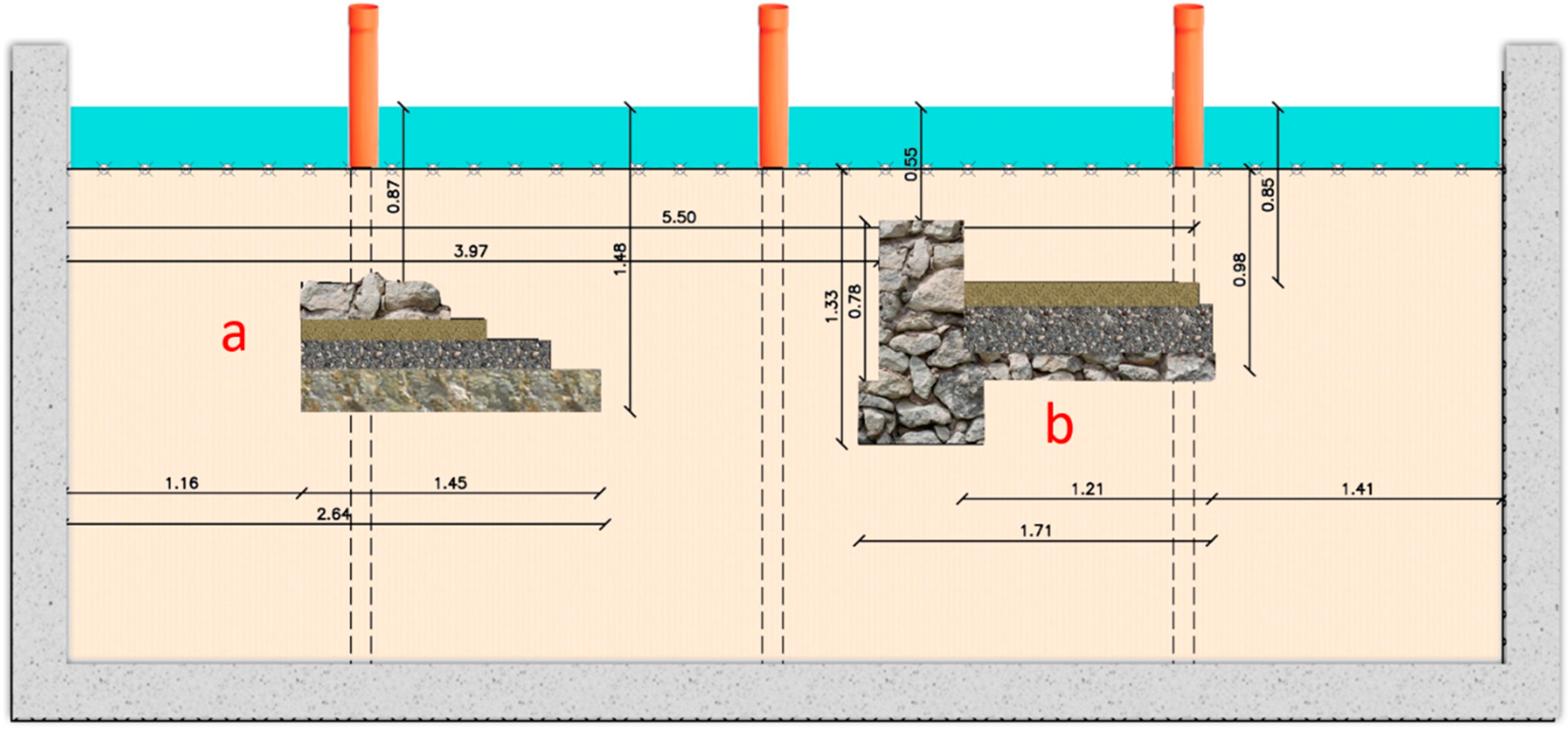
Figure 3 shows the section realized in correspondence of S1, where two targets are present. The first one is a multilayer paved road, which was placed at depth ranging between 0.90 m and 1.50 m and with horizontal extent of about 1.45 m (a). The second target is a stone wall, whose foundation and floor are placed at a depth ranging between 0.55 m and 1.65 m and with horizontal extent of about 1.71 m (b).
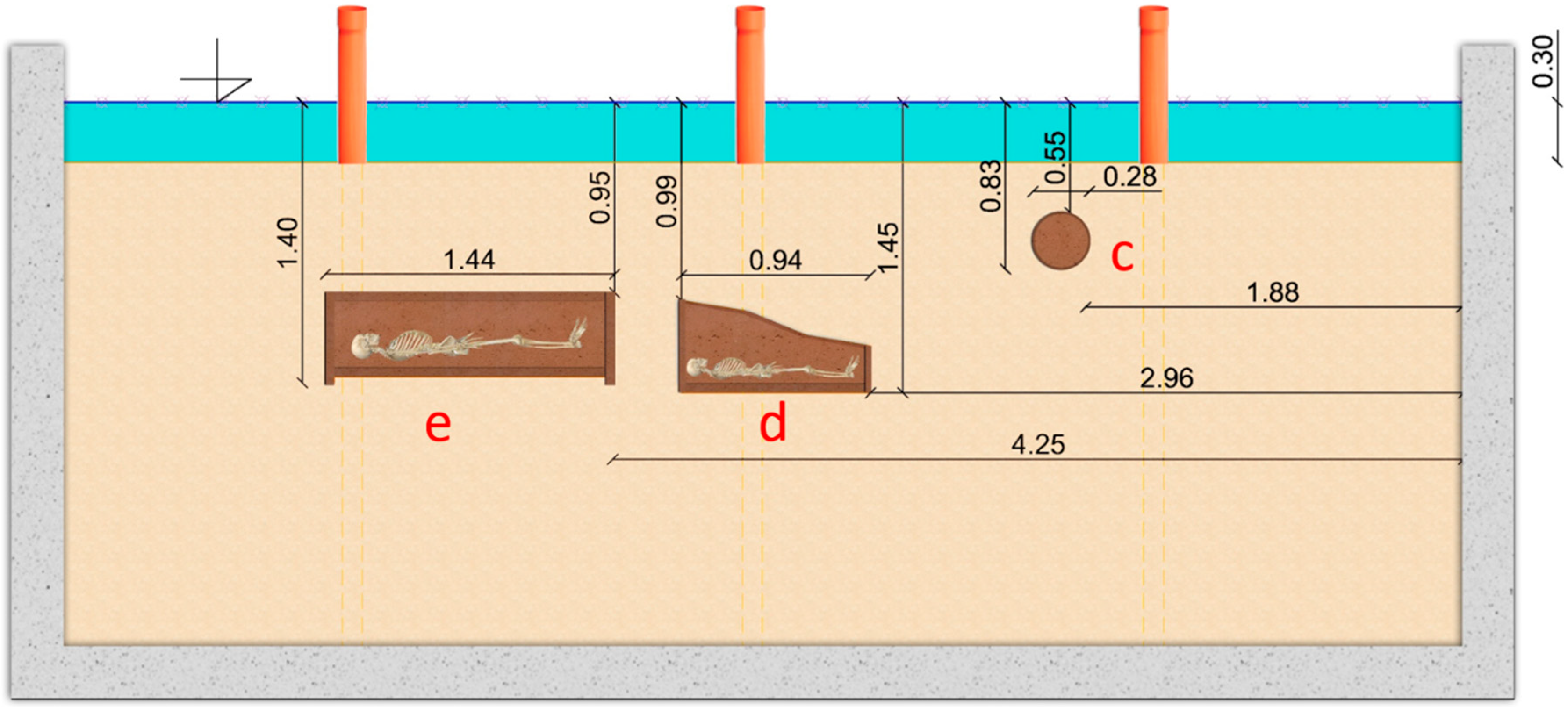
Below line S2, there are three different structures as indicated in Figure 4. The first one is an amphora (c) of irregular shape and an approximate size of 0.90 m × 0.28 m at a depth of about 0.55 m. The amphora was sealed by the mouth to make it waterproof (the object is air filled). On the same line two targets resembling tombs are placed. The first one, with size 0.95 m × 0.30 m, is characterized by a pitched roof (i.e., capuchin tomb) placed at a depth ranging between 1.00 m and 1.45 m (d); the second one is a rectangular tomb of size 0.70 m × 1.45 m approximately at depth raging between 0.95 m and 1.40 m (e). The two tombs are partially filled with the same sand present in the pool.
It is worth noting that excavation activities were made manually without the use of mechanical instruments. For this reason, the water depth profile is not levelled perfectly. To avoid the presence of micro heterogeneities, due to the excavation activities, the investigated scenario was subjected to several cycles of charge and discharge with freshwater from the bottom to the surface.
GPR surveys were performed with GPR SIR-3000 (GSSI-Instruments) equipped with a 400 MHz antenna. The antenna was placed on a small dinghy that was dragged with a system of pulleys fixed at the concrete wall of the pool that allowed us to have spatial information for the acquired data (see Figure 5). The GPR profiles were acquired by using markers placed every quarter of pulley’s wheel (equal to 0.15 m) to minimize the uncertainties in the position of the GPR antenna; the designed system has provided to acquire 100 traces at least between two markers. The transmit rate was set to 100 kHz and resolution was equal to 16 bits. No frequency filter and gain functions were adopted during data collection.
3.2. Results
This subsection is devoted to present the results obtained by processing the GPR data gathered in the pool of the Hydrogeosite Laboratory of CNR-IMAA along the lines S1 and S2 by means of the microwave tomographic approach presented in Section 2.
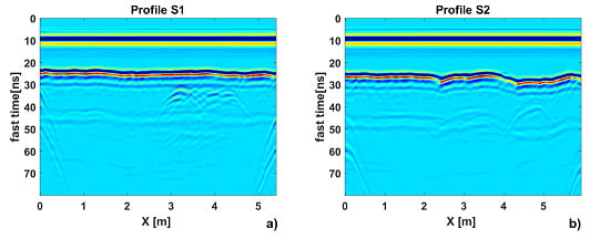
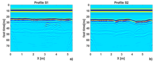
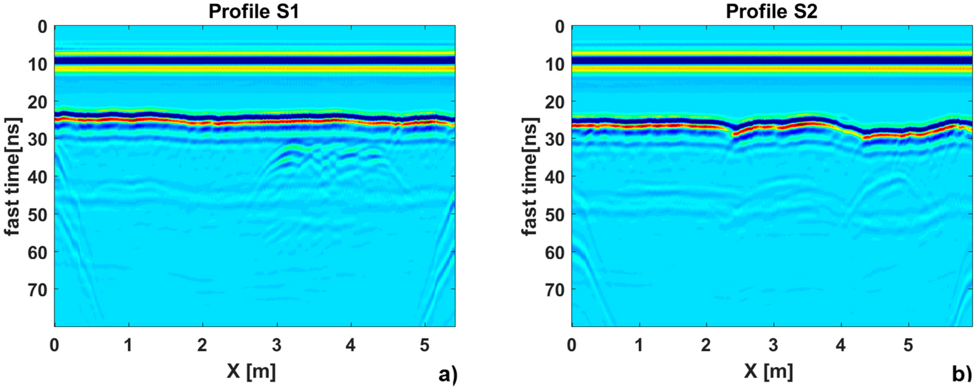
The radargrams S1 and S2 are about 5.4 m and 5.94 m long, respectively, and both are referred to a time window (two-way travel time) equal to 80 ns, discretized by means of 1024 samples. Figure 6a,b depict the raw radargrams S1 and S2, respectively. The radargrams show the direct coupling mixed with the response from the water interface at 10 ns. After, a more or less flat interface, corresponding to the freshwater-wet sand interface, appears at about 25 ns and several hyperbolas, below it, are present. A replica of the freshwater-wet sand interface appears at about 45 ns. Moreover, the radargrams show that after about 50 ns the signal is strongly attenuated.
As mentioned in the Section 3.2, the Equation (4) describes the spatial variability of the relative equivalent permittivity into the investigated domain Ω and depends on the height h of line Γ along which the antennas are moved.
As a consequence, in order to apply correctly the approximated imaging model, it is necessary to know/estimate point by point the distance between the antennas and the freshwater-wet sand interface. In this case, the antennas are located on the water surface so the above distance can be considered as bathymetry or water depth profile. Since during the experimental test no external sensors for the reconstruction of the bathymetry profile were used, this information was retrieved from data. Although the bathymetry profile can be estimated from the raw data by means of a technique based on the two-way travel time accounting for the relative dielectric permittivity of the freshwater, herein, we proposed an alternative technique by using a microwave tomographic approach formulated as for a homogeneous scenario.
Starting by applying the time domain filtering procedures, the time zero correction was performed by setting equal to 9 ns; in addition, the time window was reduced up to equal to 70 ns, for both radargrams. Moreover, we erased the signal reflections due to the borders of the pool, which are visible at the beginning and the end of the profiles in Figure 6a,b. Specifically, S1 has been reduced of 0.4 m at the beginning and 0.4 m at the end, while S2 of 0.45 m and 0.34 m, respectively. With the aim to estimate the bathymetry profile, the time gating was applied by forcing to zero the portion of the radargram external to the range from = 13 ns to = 30 ns, in order to consider only the signal due to the freshwater-wet sand interface. Figure 7a,b show the portions of the raw radargrams used to retrieve the bathymetry profile on S1 and S2, respectively.
The microwave tomographic approach was applied by assuming that the signal propagation occurred into a homogenous medium whose relative dielectric permittivity is that of the freshwater (. The effective frequency range of the data was estimated from 150 MHz to 500 MHz by means of the spectral analysis and it was sampled by 24 evenly spaced frequencies. Finally, the bathymetry profile was reconstructed by setting the TSVD threshold in such a way to filter out all of the singular values whose amplitude is 25 dB lower than the maximum one.
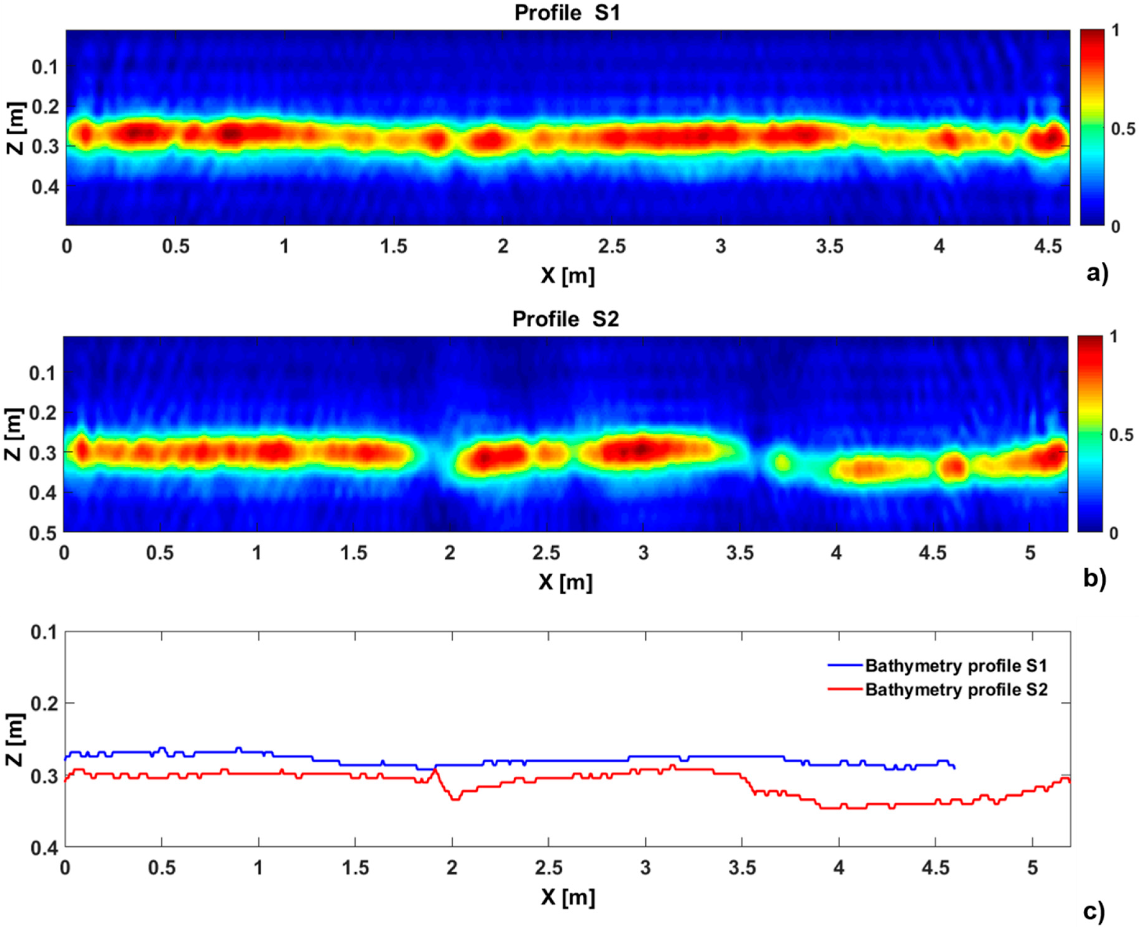
The focused images of the freshwater—wet sand interface in S1 and S2 are depicted in Figure 8a,b, respectively. Therefore, the bathymetry profiles were determined from these tomographic images by searching, for each fixed value of the abscissa , the maximum value along the -axis. Accordingly, the profiles plotted in Figure 8c were obtained.
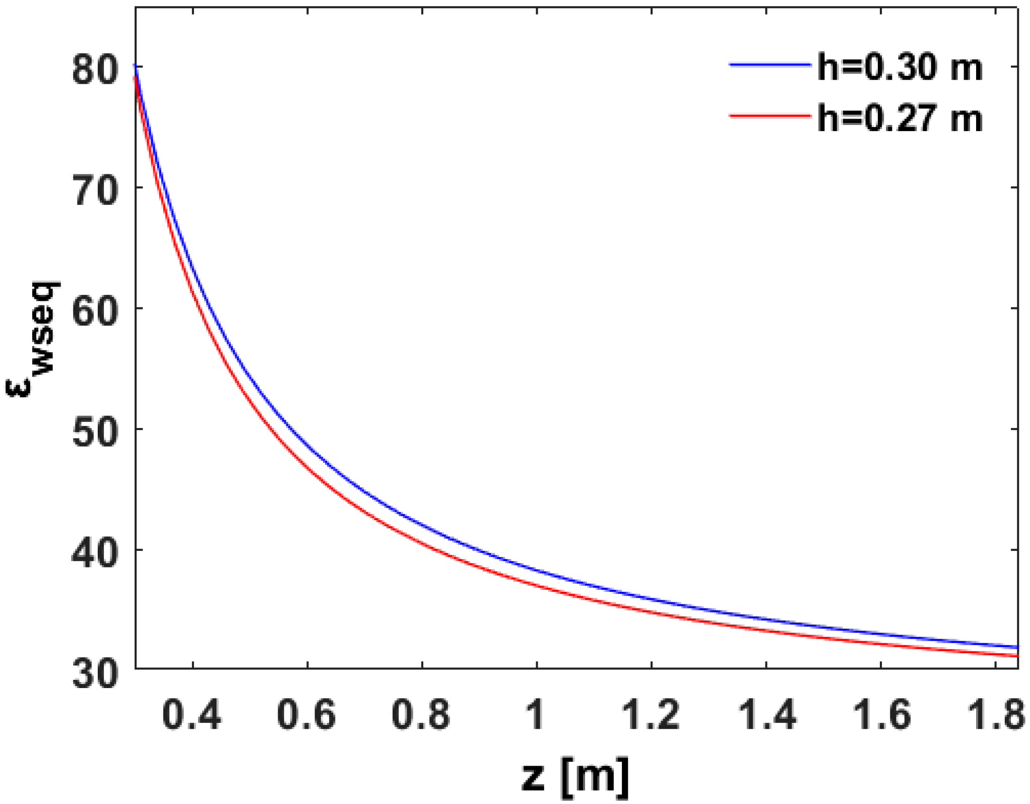
As can be observed in Figure 8c, the reconstructions of the bottom of freshwater are almost constant around the depth values 0.27 m and 0.30 m for the profile S1 and S2, respectively. These average values were used to compute the equivalent permittivity as given by Equation (4). Figure 9 shows the spatially variable behavior of along z-axis for the two considered average heights.
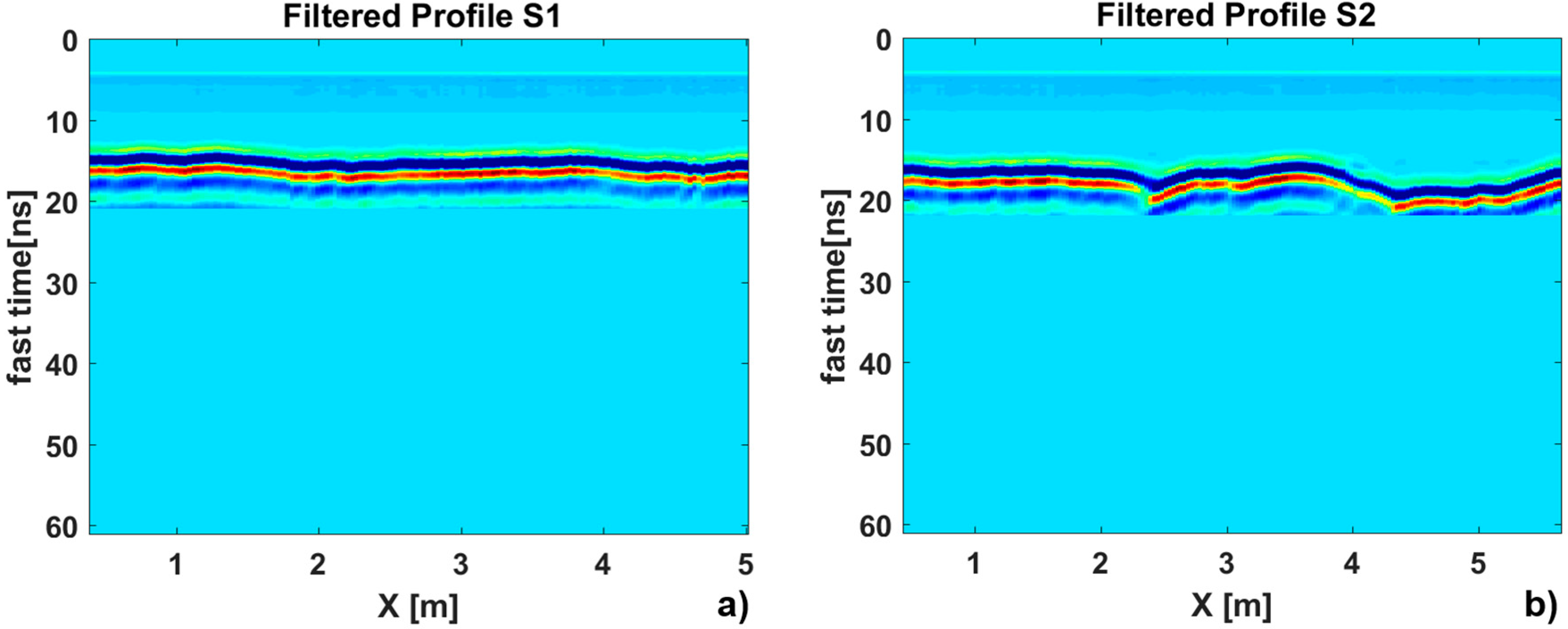
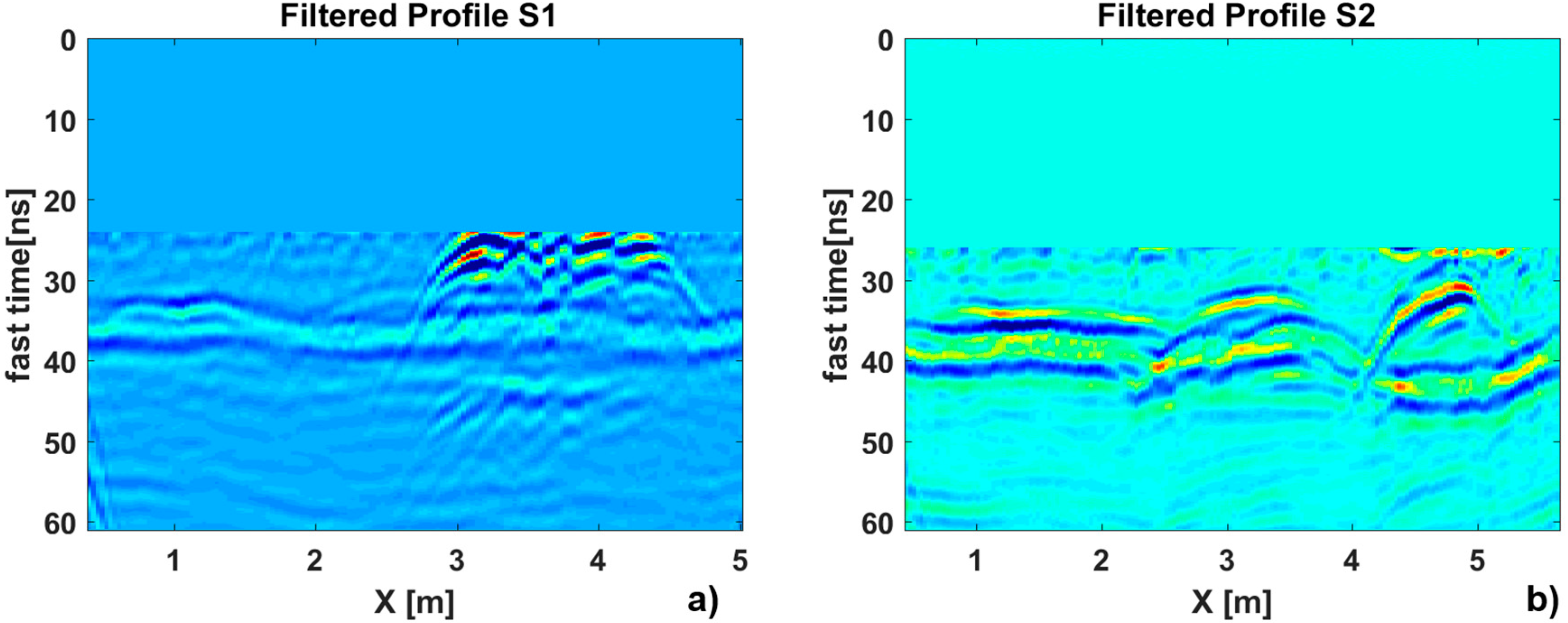
At this point, before applying the data inversion strategy to reconstruct the buried targets, we extract the useful signal portion from the radargrams S1 and S2 shown in Figure 6a,b by using the pre-processing procedure in time domain. In particular, the value of the zero-time and the reductions at the beginning and the end of the radargrams were the same as the ones adopted for the bathymetry estimation. Conversely, the direct coupling of the antennas and the freshwater-wet sand interface were removed by means of a time gating procedure considering the instant equal to 33 ns and 35 ns for the profile S1 and S2, respectively. Figure 10a,b depict the filtered radargrams related to S1 and S2, respectively.
Starting from the filtered time domain data shown in Figure 10a,b, the microwave tomographic approach was applied by considering three inversion cases:
- (i)
- homogeneous scenario with the relative dielectric permittivity of freshwater ;
- (ii)
- homogeneous scenario with the relative dielectric permittivity of wet sand ; and
- (iii)
- inversion model based on spatially equivalent permittivity .
The work frequencies as well as the threshold adopted for the TSVD inversion were the same of those considered to estimate the bathymetry profiles.
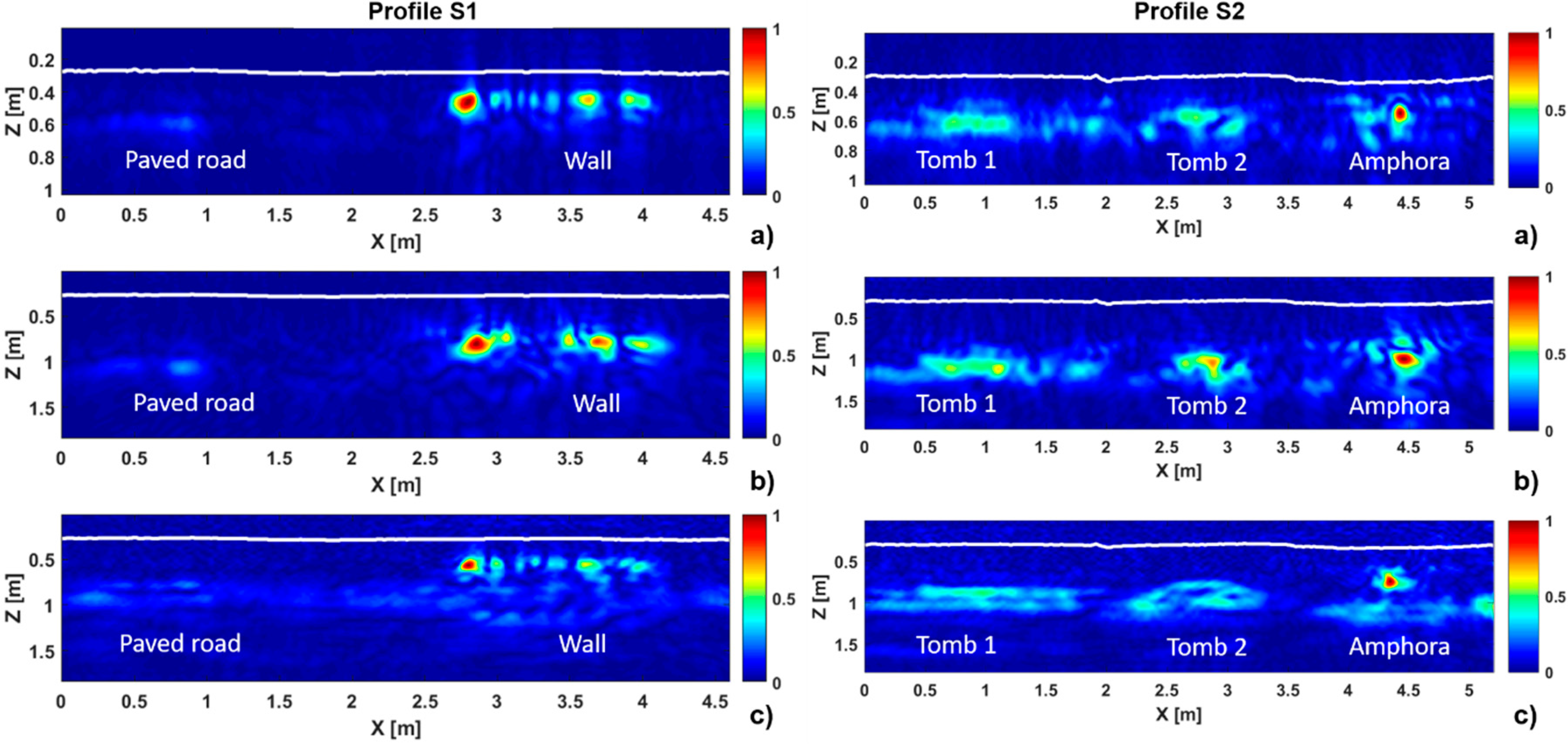
The tomographic images, for each acquisition profile S1 and S2, are shown into the left and right panels of Figure 11, respectively, and the panels (a–c) show the tomographic reconstruction obtained with relative permittivity of freshwater , wet sand , and the equivalent one , respectively. All the tomographic images in Figure 11 provide focused images of the buried ruins and allow us to gather information about their localization and size. Specifically, concerning the profile S1, the images show two localized objects identified as paved road and the archaeological wall. On the other hand, for the profile S2, the reconstructions show the presence of the two tombs and the amphora.
It is worth pointing out that, according to the Born approximation and the reflection measurement configuration adopted here, we are able to provide the information about the upper and lower sides of the targets along the z-axis, and then their vertical extension. Note that, while an accurate reconstruction of the upper side of the targets is always expected, a shift of the actual position of the lower side is foreseeable, as explained in [37], and the possibility to image it depend on the vertical spatial resolution. Moreover, the reconstructed images can be affected by ghosts due to the occurrence of multiple interactions, which are not accounted for in the approximated scattering model adopted to formulate the imaging [38].
In addition, the considered data are affected by an undesired spurious signal, which represents a replica due to the freshwater-wet sand interface (see Figure 10) and affects the tomographic images, especially for the profile S1.
4. Discussion
The results presented into the previous section corroborate that the use of microwave tomography allows us to obtain focused images of the investigated scenario, which provide precise indication about location and size of the buried objects detected in the raw radargrams of Figure 6. On the other hand, by comparing the three reconstructions shown on the left and right panels of Figure 11, one can observe that the use of a constant value for the dielectric permittivity of the investigated medium provide a less accurate localization of the objects both along the -axis and the -axis compared to the one obtained by considering a variable permittivity. In particular, we can observe that by facing the imaging problem according to the mathematical model based on the concept of equivalent permittivity it is possible to have an improved estimation both of the object size along the X-direction and estimation of their depth.
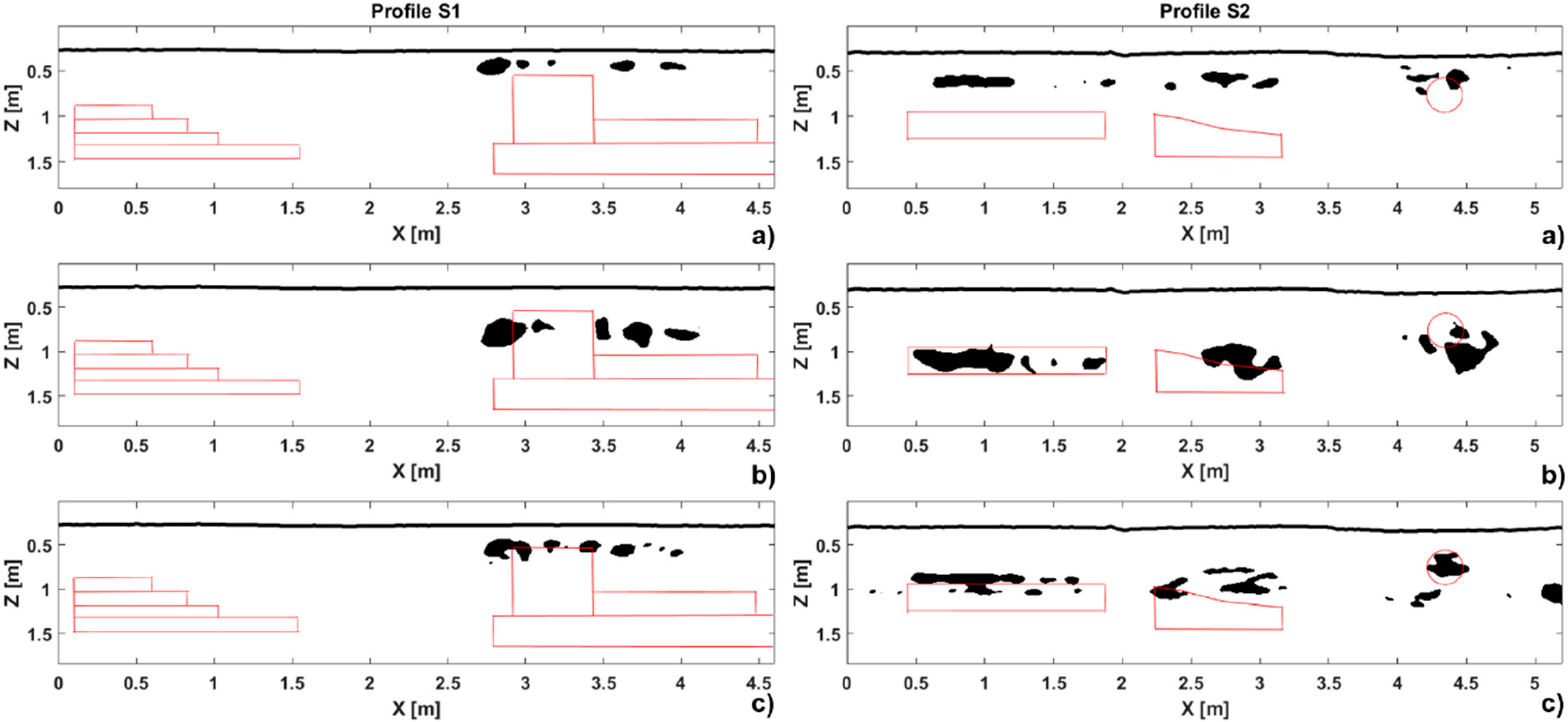
In order to support this statement, in Figure 12 left and right panels, awe reported the binary images with superimposed the boundaries of the true targets of the retrieved contrast functions referred to S1 and S2 profiles, respectively. These binary images have been obtained by using a thresholding procedure that considers as noise or artefacts the values of the amplitude of the retrieved contrast that are lower than 30% of its maximum value in the tomographic image.
It is worth noting that, as far as profile S1 is concerned, since the paved road is masked by the wall, it is not detected in left panels of the binary images in Figure 12.
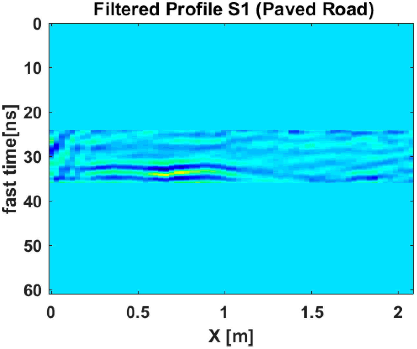
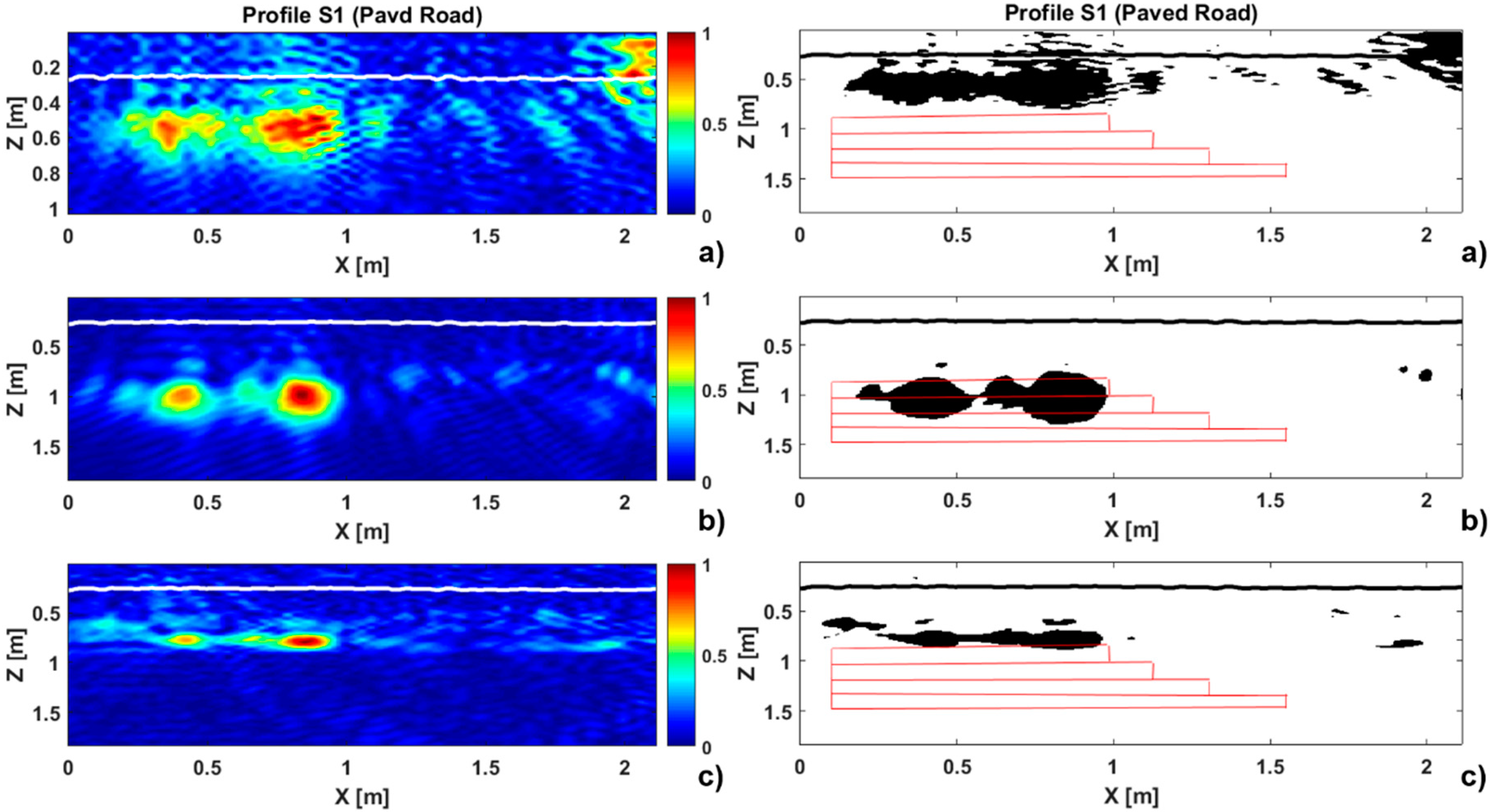
As a consequence, in order to estimate depth and extension along X-axis of the paved road, we have also elaborated only the portion of the radargram related to it, i.e., the portion of the radargram from to (see Figure 9a). In addition, the time gating was applied by forcing to zero the portion of the radargram external to the range from = 33 ns to = 45 ns, in order to emphasize the presence of the target and remove the replica due to the freshwater-wet sand interface. The filtered data concerning the paved road is shown in Figure 13.
It is worth mentioning that, also in this case, the data inversion was performed by considering the same significant spectra range, that was adopted to elaborate the entire radargram, while the threshold for the TSVD inversion was set up equal to 20 dB.
The tomographic images and the corresponding binary images are shown in Figure 14.
Table 2 reports for all the buried objects the ground truth and the retrieved values of depth, i.e., the position of the upper side, and horizontal size.
5. Conclusions
In the frame of GPR survey of underwater environments, the paper has proposed a microwave imaging approach for the detection of hidden targets located in a wet sand medium below a water layer. The proposed approach is based on a scattering model using a spatially variable equivalent permittivity and provides a three-fold advantage:
- (i)
- the layered structure of the reference scenario is taken into account without increasing the complexity of the imaging problem, which is the same of that encountered when the signal propagation occurs in a homogeneous medium;
- (ii)
- the bathymetry profile is reconstructed from the GPR data; and
- (iii)
- proper estimation of the vertical upper side location and horizontal size of the targets.
The effectiveness of the proposed imaging strategy was verified by processing experimental data collected in laboratory controlled conditions and comparing the results obtained by using a microwave tomographic approach for a homogeneous medium, whose relative dielectric permittivity was fixed equal to that of freshwater and wet sand .
The obtained results are encouraging and show that GPR can be an effective sensing technology for retrieving underwater objects. Moreover, although the use of a microwave tomographic approach formulated for a homogeneous reference scenario allows detection and localization of the targets, the introduction of a scattering model using a spatially variable dielectric permittivity provides better results in terms of localization and size reconstruction.
Future activities are addressed towards an extensive analysis of the achievable imaging capabilities in terms of detection and localization of the submerged targets. First of all, more complex scenarios, where the targets are submerged at a higher depth than that considered in this paper and lake or sea water is present, will be taken into account. Since, in the presence of sea water, a significant attenuation of the useful signal is foreseeable, we point out that a procedure aimed at compensating for this attenuation is expected to be necessary in the pre-processing step of the inversion strategy. Moreover, the presence of micro-heterogeneities of the surveyed environment will be considered and a comparison with the results obtained by considering a more sophisticated representation of the reproduced scenario into the scattering model will be performed.
Author Contributions
G.L. worked on data processing, interpretation of the results, and the writing of the paper. I.C. and F.S. derived the proposed scattering model. Moreover, I.C. collaborated to the interpretation of the results and the writing of the paper, while F.S. reviewed the results and the paper. L.C. and E.R. realized the laboratory test site and performed the GPR surveys. In addition, L.C. contributed in writing the test site description and E.R. reviewed it.
Funding
This research was funded by the European Union’s Horizon 2020 research and innovation program under grant agreement No. 700395.
Conflicts of Interest
The authors declare no conflict of interest.
References
- Daniels, D.J. Ground Penetrating Radar. In IEE Radar, Sonar and Navigation Series 15; IEE: London, UK, 2004. [Google Scholar] [Green Version]
- Persico, R. Introduction to Ground Penetrating Radar: Inverse Scattering and Data Processing; Wiley-IEEE Press: London, UK, 2014. [Google Scholar]
- Conyers, L.B.; Goodman, D. Ground-Penetrating Radar: An Introduction for Archaeologists; AltaMira Press: Walnut Creek, CA, USA, 1997. [Google Scholar]
- Masini, N.; Capozzoli, L.; Chen, P.; Chen, F.; Romano, G.; Lu, P.; Tang, P.; Sileo, M.; Ge, Q.; Lasaponara, R. Towards an Operational Use of Geophysics for Archaeology in Henan (China): Methodological Approach and Results in Kaifeng. Remote Sens. 2017, 9, 809. [Google Scholar] [CrossRef]
- Rizzo, E.; Santoriello, A.; Capozzoli, L.; De Martino, G.; De Vita, C.B.; Musmeci, D.; Perciante, F. Geophysical survey and archaeological data at Masseria Grasso (Benevento, Italy). Surv. Geophys. 2018. [Google Scholar] [CrossRef]
- Capozzoli, L.; Rizzo, E. Combined NDT techniques in civil engineering applications: Laboratory and real tests. Constr. Build. Mater. 2017, 154, 1139–1150. [Google Scholar] [CrossRef]
- Beben, D.; Mordak, A.; Anigacz, W. Identification of viaduct beam parameters using the Ground Penetrating Radar (GPR) technique. NDT E Int. 2012, 49, 18–26. [Google Scholar] [CrossRef]
- De Chiara, F.; Fontul, S.; Fortunato, E. GPR Laboratory Tests for Railways Materials Dielectric Properties Assessment. Remote Sens. 2014, 6, 9712–9728. [Google Scholar] [CrossRef]
- Orlando, L.; Pezone, A.; Colucci, A. Modeling and testing of high frequency GPR data for evaluation of structural deformation. NDT E Int. 2010, 43, 216–230. [Google Scholar] [CrossRef]
- Catapano, I.; Ludeno, G.; Soldovieri, F.; Tosti, F.; Padeletti, G. Structural Assessment via Ground Penetrating Radar at the Consoli Palace of Gubbio (Italy). Remote Sens. 2017, 10, 45. [Google Scholar] [CrossRef]
- Hellsten, H. CARABAS—An UWB low frequency SAR. In Proceedings of the IEEE MTT-S International Symposium, Albuquerque, NM, USA, 1–5 June 1992; Volume 3, pp. 1495–1498. [Google Scholar]
- Catapano, I.; Crocco, L.; Krellmann, Y.; Triltzsch, G.; Soldovieri, F. A tomographic approach for helicopter-borne ground penetrating radar imaging. IEEE Geosci. Remote Sens. Lett. 2012, 9, 378–382. [Google Scholar] [CrossRef]
- Papa, C.; Alberti, G.; Salzillo, G.; Palmese, G.; Califano, D.; Ciofaniello, L.; Daniele, M.; Facchinetti, C.; Longo, F.; Formaro, R.; et al. Design and Validation of a Multimode Multifrequency VHF/UHF Airborne Radar. IEEE. Geosci. Remote Sens. Lett. 2014, 11, 1260–1264. [Google Scholar] [CrossRef]
- Ludeno, G.; Catapano, I.; Renga, A.; Rodi Vetrella, A.; Fasano, G.; Soldovieri, F. Assessment of a micro-UAV system for microwave tomography radar imaging. Remote Sens. Environ. 2018, 212, 90–102. [Google Scholar] [CrossRef]
- Eisenburger, D.; Krellmann, Y.; Lentz, H.; Triltzsch, G. Stepped frequency radar system in gating mode: An experiment as a new helicopter-borne GPR systems for geological applications. In Proceedings of the IGARSS 2008—2008 IEEE International Geoscience and Remote Sensing Symposium, Boston, MA, USA, 7–11 July 2008; pp. I153–I156. [Google Scholar]
- Travassos, J.D.M.; Menezes, P.D.T.L. GPR exploration for groundwater in a crystalline rock terrain. J. Appl. Geophys. 2004, 55, 239–248. [Google Scholar] [CrossRef]
- Machguth, H.; Eisen, O.; Paul, F.; Hoelzle, M. Strong spatial variability of snow accumulation observed with helicopter-borne GPR on two adjacent Alpine glaciers. Geophys. Res. Lett. 2006, 33, L13. [Google Scholar] [CrossRef]
- Negi, H.S.; Snehmani, N.T.; Sharma, J.K. Estimation of snow depth and detection of buried objects using airborne ground penetrating radar in Indian Himalaya. Curr. Sci. 2008, 94, 865–870. [Google Scholar]
- Catapano, I.; di Napoli, R.; Soldovieri, F.; Bavusi, M.; Loperte, A.; Dumoulin, J. Structural monitoring via microwave tomography-enhanced GPR: The Montagnole test site. J. Geophys. Eng. 2012, 9, S100. [Google Scholar] [CrossRef]
- Hasan, I.; Yazdani, N. Ground penetrating radar utilization in exploring inadequate concrete covers in a new bridge deck. Case Stud. Constr. Mater. 2014, 1, 104–114. [Google Scholar] [CrossRef]
- Chang, C.W.; Lin, C.H.; Lien, H.S. Measurement radius of reinforcing steel bar in concrete using digital image GPR. Constr. Build. Mater. 2009, 23, 1057–1063. [Google Scholar] [CrossRef]
- Hugenschmidt, J.; Mäder, A. GPR investigation of remains of pile dwellings in Lake Zurich. In Proceedings of the 2018 17th International Conference on Ground Penetrating Radar (GPR), Rapperswil, Switzerland, 18–21 June 2018; pp. 1–4. [Google Scholar]
- The Impacts of Climate Change on World Heritage Properties. Available online: https:\\whc.unesco.org\document\7041 (accessed on 31 August 2018).
- Xu, X.; Wu, J.; Shen, J.; He, Z. Case Study: Application of GPR to Detection of Hidden Dangers to Underwater Hydraulic Structures. J. Hydraul. Eng. 2006, 1, 12–20. [Google Scholar] [CrossRef]
- Diamanti, N.; Giannopoulos, A.; Forde, M.C. Numerical modelling and experimental verification of GPR to investigate ring separation in brick masonry arch bridges. NDT E Int. 2008, 41, 354–363. [Google Scholar] [CrossRef]
- Soldovieri, F.; Hugenschmidt, J.; Persico, R.; Leone, G. A linear inverse scattering algorithm for realistic GPR applications. Near Surf. Geophys. 2007, 5, 29–42. [Google Scholar] [CrossRef]
- Catapano, I.; Affinito, A.; Gennarelli, G.; di Maio, F.; Loperte, A.; Soldovieri, F. Full three-dimensional imaging via ground penetrating radar: Assessment in controlled conditions and on field for archaeological prospecting. Appl. Phys. A 2013, 115, 1415–1422. [Google Scholar] [CrossRef]
- Lopez-Sanchez, J.M.; Fortuny-Guasch, J. 3-D radar imaging using range migration techniques. IEEE Trans. Antennas Propag. 2000, 48, 728–737. [Google Scholar] [CrossRef]
- Soldovieri, F.; Crocco, L. Electromagnetic Tomography. In Vertiy Subsurface Sensing; Ahmet, S., Turk Koksal, A., Hocaoglu Alexey, A., Eds.; Wiley: Hoboken, NJ, USA, 2011. [Google Scholar]
- Catapano, I.; Ludeno, G.; Soldovieri, F. An approximated imaging approach for GPR surveys with antennas far from the interface. In Proceedings of the 2017 9th International Workshop on Advanced Ground Penetrating Radar (IWAGPR), Edinburgh, UK, 28–30 June 2017; pp. 1–5. [Google Scholar]
- Leone, G.; Soldovieri, F. Analysis of the Distorted Born Approximation for Subsurface Reconstruction: Truncation and Uncertainties Effects. IEEE Trans. Geosci. Remote Sens. 2003, 41, 66–74. [Google Scholar] [CrossRef]
- Capozzoli, L.; Caputi, A.; De Martino, G.; Giampaolo, V.; Luongo, R.; Perciante, F.; Rizzo, E. Electrical and electromagnetic techniques applied to an archaeological framework reconstructed in laboratory. In Proceedings of the 2015 8th IEEE IWAGPR, Advanced Ground Penetrating Radar, Florence, Italy, 7–10 July 2015. [Google Scholar]
- Bertero, M.; Boccacci, P. Introduction to Inverse Problems in Imaging; Institute of Physics Publications: London, UK, 1998. [Google Scholar]
- Felsen, L.B.; Marcuvitz, N. Radiation and Scattering of Waves; Wiley: New York, NY, USA, 2003. [Google Scholar]
- Balanis, A.C. Advanced Engineering Electromagnetics; John Wiley & Sons: New York, NY, USA, 2012; Volume 111. [Google Scholar]
- Capozzoli, L.; De Martino, G.; Perciante, F.; Rizzo, E. Geophysical techniques applied to investigate underwater structures. In Proceedings of the 9th International Workshop on Advanced Ground Penetrating Radar (IWAGPR), Edinburgh, UK, 28–30 June 2017; pp. 1–5. [Google Scholar]
- Pettinelli, E.; Di Matteo, A.; Mattei, E.; Crocco, L.; Soldovieri, F.; Redman, J.D.; Annan, A.P. GPR Response From Buried Pipes: Measurement on Field Site and Tomographic Reconstructions. IEEE Trans. Geosci. Remote Sens. 2009, 47, 2639–2645. [Google Scholar] [CrossRef]
- Persico, R.; Bernini, R.; Soldovieri, F. The Role of the Measurement Configuration in Inverse Scattering From Buried Objects under the Born Approximation. IEEE Trans. Antennas Propag. 2005, 53, 1875–1887. [Google Scholar] [CrossRef]
Figure 1.
Reference scenario.

Figure 2.
Plan of the investigated site with indication of the archaeological structures placed into wet sand: (a) wall; (b) paved road; (c) amphora; (d) capuchin tomb; (e) rectangular tomb.
Figure 2.
Plan of the investigated site with indication of the archaeological structures placed into wet sand: (a) wall; (b) paved road; (c) amphora; (d) capuchin tomb; (e) rectangular tomb.

Figure 3.
Transversal section realized on the line S1 with an indication of the size and depth of the buried objects.
Figure 3.
Transversal section realized on the line S1 with an indication of the size and depth of the buried objects.

Figure 4.
Transversal section realized on the line S2 with an indication of the size and depth of the buried objects.
Figure 4.
Transversal section realized on the line S2 with an indication of the size and depth of the buried objects.

Figure 5.
Photo of the investigated site with GPR system used for the acquisition without a survey wheel.
Figure 5.
Photo of the investigated site with GPR system used for the acquisition without a survey wheel.

Figure 6.
Raw radargram collected along S1 (a) and S2 (b) profiles.

Figure 7.
Filtered radargram used to retrieve the bathymetry referred to S1 (a) and S2 (b).

Figure 8.
Tomographic images of the freshwater-wet sand interface related to profile S1 (a) and S2 (b); bathymetry reconstruction related to profile S1 (blue line) and S2 (red lines) (c). The tomographic images show the normalized intensity of the retrieved contrast.
Figure 8.
Tomographic images of the freshwater-wet sand interface related to profile S1 (a) and S2 (b); bathymetry reconstruction related to profile S1 (blue line) and S2 (red lines) (c). The tomographic images show the normalized intensity of the retrieved contrast.

Figure 9.
Behavior of the equivalent dielectric permittivity along z-axis for the height h = 0.30 m (blue line) and h = 0.27 m (red line).
Figure 9.
Behavior of the equivalent dielectric permittivity along z-axis for the height h = 0.30 m (blue line) and h = 0.27 m (red line).

Figure 10.
Filtered radargram obtained by means of pre-processing procedure associated to the profile S1 (a) and S2 (b).
Figure 10.
Filtered radargram obtained by means of pre-processing procedure associated to the profile S1 (a) and S2 (b).

Figure 11.
Tomographic images for each profile S1 (left panels) and S2 (right panels); panels (a–c) show the tomographic reconstruction obtained with relative permittivity of the freshwater , the wet sand , and the equivalent one , respectively. The white lines represent the estimated bathymetry profiles. The tomographic images show the normalized intensity of the retrieved contrast.

Figure 12.
Binary images of the tomographic images with superimposed in red the boundaries of the true targets. panels (a–c) show the binary images of the tomographic images obtained with relative permittivity of the freshwater , the wet sand , and the equivalent one , respectively.
Figure 12.
Binary images of the tomographic images with superimposed in red the boundaries of the true targets. panels (a–c) show the binary images of the tomographic images obtained with relative permittivity of the freshwater , the wet sand , and the equivalent one , respectively.

Figure 13.
Portion of the radargram related to the paved road.

Figure 14.
Portion of the tomographic (left panels) and binary (right panels) images related to the buried paved road in the profile S1; panels (a–c) shown the tomographic reconstruction obtained with relative permittivity of the freshwater , the wet sand , and that equivalent , respectively. The white lines represent the bathymetry profiles. The tomographic images show the normalized intensity of the retrieved contrast. The boundaries of the true paved road are superimposed in red on the binary images.


Table 1.
Chemical and hydrogeological parameters of the sand used for the experiment. dm, Kmax, and ρ represent average diameter of the sand, hydraulic conductivity and porosity, respectively.
Table 1.
Chemical and hydrogeological parameters of the sand used for the experiment. dm, Kmax, and ρ represent average diameter of the sand, hydraulic conductivity and porosity, respectively.
| Chemical Results | ||||||
|---|---|---|---|---|---|---|
| SiO2 | Al2O3 | Fe2O3 | CaO | K2O | ||
| % | 93.00 | 2.50 | 0.60 | 1.50 | 1.15 | |
| Particle Size Characteristics d (mm) | ||||||
| d (mm) | 1–0.5 | 0.50–0.25 | 0.250–0.125 | 0.125–0.063 | 0.063–0.032 | >0.032 |
| % | 0.00 | 0.14 | 3.70 | 86.34 | 7.92 | 1.08 |
| Hydrogeological Properties | ||||||
| dm (mm) | Kmax (m/s) | ρ (%) | ||||
| 0.09 | 4 × 10⁻⁵ | 45–50 | ||||
Table 2.
Values of the all buried objects for both considered profiles in terms of upper side location (depth zt (m)) and horizontal size ( (m)).
Table 2.
Values of the all buried objects for both considered profiles in terms of upper side location (depth zt (m)) and horizontal size ( (m)).
| Profile S1 | Profile S2 | |||||||||
|---|---|---|---|---|---|---|---|---|---|---|
| Paved Road | Wall | Tomb 1 | Tomb 2 | Amphora | ||||||
| zt (m) | (m) | zt (m) | (m) | zt (m) | (m) | zt (m) | (m) | zt (m) | (m) | |
| Ground-truth | 0.77 | 1.45 | 0.55 | 1.71 | 0.95 | 1.44 | 0.99 | 0.94 | 0.80 | 0.28 |
| 0.58 | 0.85 | 0.40 | 1.37 | 0.60 | 0.56 | 0.57 | 0.59 | 0.54 | 0.24 | |
| 1.06 | 0.80 | 0.75 | 1.40 | 1.05 | 0.70 | 1.00 | 0.37 | 1.00 | 0.45 | |
| 0.78 | 0.96 | 0.52 | 1.30 | 0.86 | 1.24 | 0.77 | 0.86 | 0.74 | 0.34 | |
© 2018 by the authors. Licensee MDPI, Basel, Switzerland. This article is an open access article distributed under the terms and conditions of the Creative Commons Attribution (CC BY) license (http://creativecommons.org/licenses/by/4.0/).
Share and Cite
MDPI and ACS Style
Ludeno, G.; Capozzoli, L.; Rizzo, E.; Soldovieri, F.; Catapano, I. A Microwave Tomography Strategy for Underwater Imaging via Ground Penetrating Radar. Remote Sens. 2018, 10, 1410. https://0-doi-org.brum.beds.ac.uk/10.3390/rs10091410
AMA Style
Ludeno G, Capozzoli L, Rizzo E, Soldovieri F, Catapano I. A Microwave Tomography Strategy for Underwater Imaging via Ground Penetrating Radar. Remote Sensing. 2018; 10(9):1410. https://0-doi-org.brum.beds.ac.uk/10.3390/rs10091410
Chicago/Turabian StyleLudeno, Giovanni, Luigi Capozzoli, Enzo Rizzo, Francesco Soldovieri, and Ilaria Catapano. 2018. "A Microwave Tomography Strategy for Underwater Imaging via Ground Penetrating Radar" Remote Sensing 10, no. 9: 1410. https://0-doi-org.brum.beds.ac.uk/10.3390/rs10091410
Note that from the first issue of 2016, this journal uses article numbers instead of page numbers. See further details here.