Hyperspectral Dimensionality Reduction Based on Multiscale Superpixelwise Kernel Principal Component Analysis


1
Chongqing Engineering Research Center for Remote Sensing Big Data Application, School of Geography Science, Southwest University, Chongqing 400715, China
2
State Cultivation Base of Eco-agriculture for Southwest Mountainous Land, Southwest University, Chongqing 400715, China
3
School of Earth Sciences and Engineering, Hohai University, Nanjing 211100, China
*
Author to whom correspondence should be addressed.
Remote Sens. 2019, 11(10), 1219; https://0-doi-org.brum.beds.ac.uk/10.3390/rs11101219
Submission received: 26 April 2019
/
Revised: 17 May 2019
/
Accepted: 20 May 2019
/
Published: 23 May 2019
(This article belongs to the Special Issue Dimensionality Reduction for Hyperspectral Imagery Analysis)
Abstract
:Dimensionality reduction (DR) is an important preprocessing step in hyperspectral image applications. In this paper, a superpixelwise kernel principal component analysis (SuperKPCA) method for DR that performs kernel principal component analysis (KPCA) on each homogeneous region is proposed to fully utilize the KPCA’s ability to acquire nonlinear features. Moreover, for the proposed method, the differences in the DR results obtained based on different fundamental images (the first principal components obtained by principal component analysis (PCA), KPCA, and minimum noise fraction (MNF)) are compared. Extensive experiments show that when 5, 10, 20, and 30 samples from each class are selected, for the Indian Pines, Pavia University, and Salinas datasets: (1) when the most suitable fundamental image is selected, the classification accuracy obtained by SuperKPCA can be increased by 0.06%–0.74%, 3.88%–4.37%, and 0.39%–4.85%, respectively, when compared with SuperPCA, which performs PCA on each homogeneous region; (2) the DR results obtained based on different first principal components are different and complementary. By fusing the multiscale classification results obtained based on different first principal components, the classification accuracy can be increased by 0.54%–2.68%, 0.12%–1.10%, and 0.01%–0.08%, respectively, when compared with the method based only on the most suitable fundamental image.
1. Introduction
Hyperspectral imagery (HSI) typically contains hundreds of narrow-band radiation information, which provides more discriminative features for feature recognition or classification. However, the spectral values of adjacent bands in hyperspectral images usually have a strong correlation [1], and the high spectral resolution makes the data redundant and generates a “dimension disaster” problem during supervised learning [2]. This effect makes dimensionality reduction an important preprocessing step in hyperspectral image applications.
Principal component analysis (PCA) is one of the most widely used unsupervised dimensionality reduction models [3]. The principal components (PCs) obtained by PCA are linearly independent and are sorted by variance in descending order. Information mainly exists in the first few PCs. However, as a linear orthogonal transform method, it is difficult for PCA to handle the complex nonlinear characteristics in HSIs. These nonlinear characteristics are mainly derived from various nonlinear factors in the imaging process, such as nonlinear scattering from the bidirectional reflectance distribution function (BRDF) and electromagnetic wave interference of adjacent objects [4,5].
Among several nonlinear extensions of PCA [6,7,8,9], kernel PCA (KPCA) [9] uses a kernel function to nonlinearly map the original data to a high-dimensional feature space, and by performing PCA in the high-dimensional feature space, the nonlinear dimensionality reduction is subtly realized. In addition to inheriting several related properties from PCA, KPCA does not suffer from some practical problems faced by other nonlinear PCA extensions, such as nonconvergence or convergence to local minima [10]. KPCA and its extensions have proven to be powerful tools for feature extraction and image denoising [10,11,12,13,14,15,16,17].
On the other hand, image segmentation technology has been widely used in the field of image classification, as it can simultaneously utilize spatial and spectral information of HSIs [18,19,20,21,22,23,24,25,26]. By segmenting the image into multiple homogeneous regions and performing corresponding operations on each homogeneous region, the classification performance can be greatly improved. Since the real surface is extremely complicated in most cases, it is sometimes difficult for a single segmentation algorithm or a single segmentation scale to make full use of the rich spatial information in HSIs. Therefore, the strategy of fusing the classification results obtained by different segmentation algorithms [27] and the strategy of fusing the classification results of different segmentation scales [28,29,30,31,32] can generally improve the classification accuracy.
Recently, the strategy of fusing the classification results based on multiscale segmentation has been applied to the field of dimensionality reduction and has achieved competitive results [33]. A real surface usually contains multiple homogeneous regions. Dimensionality reduction based only on the globally optimal projection direction tends to ignore the difference between different homogeneous regions, and at the same time, different homogeneous regions are usually of different sizes, so it is usually difficult for a single segmentation scale to accurately capture the difference in size between these different homogeneous regions. To solve these problems, Jiang et al. proposed segmenting HSI into superpixels of multiple scales. By performing PCA on each superpixel of each scale, the low-dimensional representations of HSI at different scales are obtained. The final classification result is obtained by fusing the classification results of each scale using the majority voting (MV) decision fusion strategy. This method was named multiscale segmentation-based superpixelwise PCA (MSuperPCA) by Jiang et al., and the method based on single-scale segmentation was named superpixelwise PCA (SuperPCA). Extensive experiments show that the low-dimensional representation obtained by performing PCA on each superpixel is separable, compact, and anti-noise, leading to an improvement in classification accuracy [33].
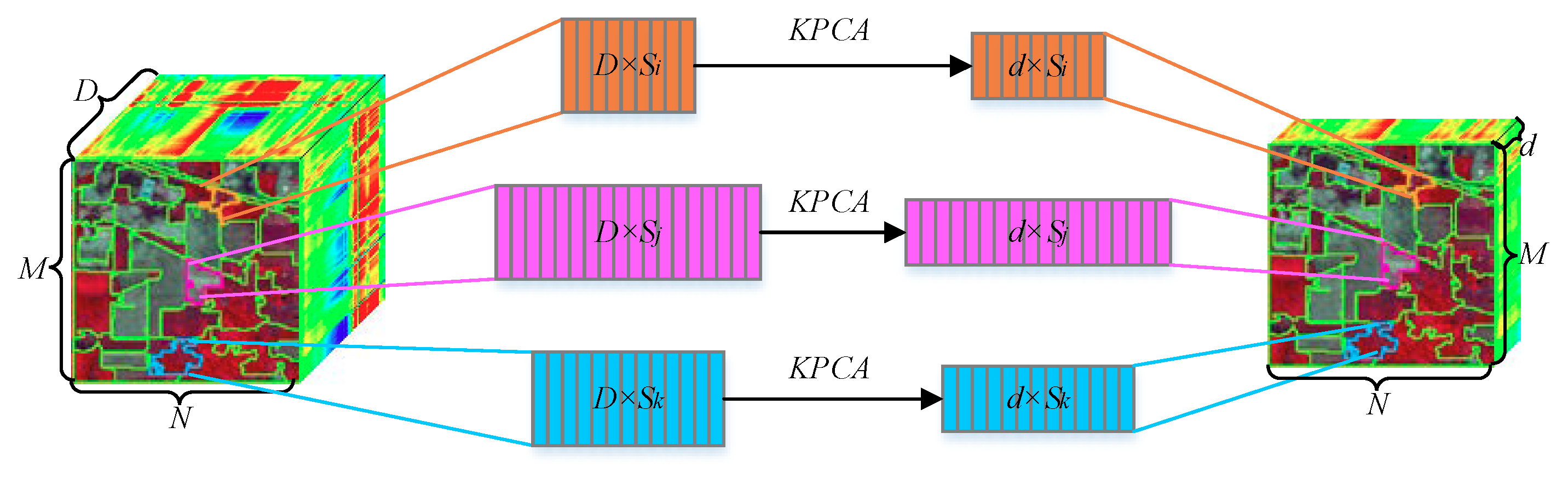
However, as mentioned earlier, PCA cannot handle the nonlinear characteristics prevalent in HSIs. Therefore, a method called superpixelwise KPCA (SuperKPCA) is proposed to make full use of the advantages of KPCA in obtaining nonlinear low-dimensional representation of images, and to make full use of the advantages of image segmentation technology in acquiring different homogeneous regions and improving the classification performance. More specifically, image segmentation technology is first used to acquire homogeneous regions, and then KPCA is used to reduce the dimensionality of each homogeneous region to obtain a more accurate nonlinear low-dimensional representation of the hyperspectral image. The specific implementation process is shown in Figure 1. Each of the homogeneous regions is represented by a matrix, and the columns of the matrix represent spectral vectors of the pixels.
Since classification performance can be further improved by fusing the classification results after multiscale segmentation, the multiscale segmentation strategy is used in this article to make better use of the spatial information of different homogeneous regions. By extracting the same kernel PCs for each homogeneous region (superpixel) under each segmentation scale, the nonlinear low-dimensional features of HSI at different segmentation scales are obtained. Finally, the support vector machine (SVM) [34,35] is used to classify the low-dimensional representations at different scales. By using the majority voting decision fusion strategy to fuse the classification results of each scale, the final classification result is obtained. For the convenience of writing, the above method is named multiscale segmentation-based SuperKPCA (MSuperKPCA).
An HSI usually contains hundreds of bands, but the input of most image segmentation algorithms is usually a grayscale image or an RGB image. Therefore, most studies select the first PC obtained by PCA as the fundamental image for segmentation [29,30,31,33]. Although the first PC can contain the main information of the hyperspectral image, the second and third PCs usually contain some useful information. Therefore, in some studies, the first three PCs obtained by PCA are regarded as the three bands of the color image and are used as the fundamental image for segmentation [18,22]. However, since the second and third PCs may contain noise while containing useful information, there is still room for improvement in the classification accuracy of these studies.
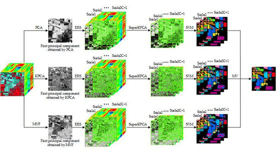
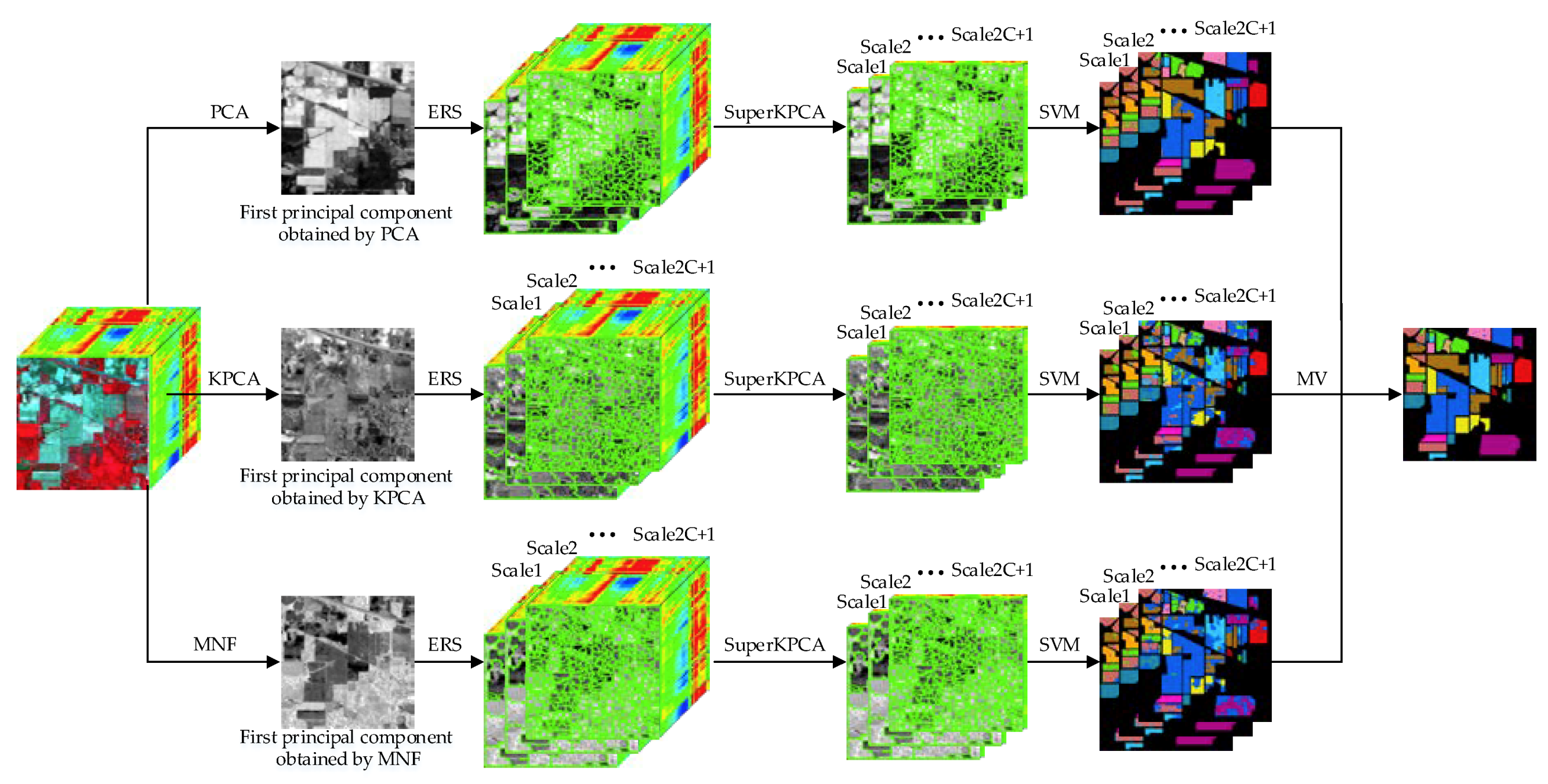
It is well known that the PCs obtained by PCA and KPCA are arranged in descending order of the magnitude of the eigenvalues, and the PCs obtained by minimum noise fraction (MNF) transformation are sorted according to the image quality [36]. Usually, the first PC contains most of the information of a hyperspectral image. That is, the first PCs obtained by the three algorithms represent different main information of a hyperspectral image. Therefore, the segmentation results obtained based on different first PCs can be different, and correspondingly, dimensionality reduction and classification results can also be different. Inspired by the multiclassifier strategy [27], this study attempts to fuse the classification results based on different fundamental images. First, the first PCs obtained by PCA, KPCA, and MNF are obtained; second, each of the first PCs are treated as a fundamental image, and multiscale segmentation, dimensionality reduction, and classification (using SVM) are performed. Finally, the majority voting decision fusion strategy is used to fuse all the classification results. For the convenience of writing, this idea is referred to as 3-MSuperKPCA. The specific implementation process is shown in Figure 2.
To the best of our knowledge, the extension of KPCA to the field of superpixel segmentation and its use for unsupervised dimensionality reduction is rarely seen in previous studies. Extensive experiments have shown that by segmenting the hyperspectral image into multiple homogeneous regions and performing KPCA on each homogeneous region separately, the proposed superpixel-based KPCA method is superior to the superpixel-based PCA method in most cases, whether it is based on single-scale segmentation or multiscale segmentation. At the same time, as far as we know, in the field of superpixel-based unsupervised dimensionality reduction, the influence of different fundamental images on dimensionality reduction results has rarely been studied. Extensive experiments have shown that the dimensionality reduction results obtained based on different fundamental images are different and complementary for the proposed method, and by fusing multiscale classification results based on different fundamental images, the classification performance can often be further improved.
2. Proposed Methods
2.1. Multiscale Superpixel Segmentation
As a preprocessing step, the superpixel segmentation algorithm needs to have a lower computational complexity while adhering well to the boundary of the features. The existing methods for generating superpixels mainly include two types: gradient-based methods [37,38,39] and graph-based methods [40,41,42,43]. In this paper, the entropy rate segmentation (ERS) [40] algorithm is adopted to generate a 2-D superpixel map due to its promising performance in both efficacy and efficiency. The ERS algorithm is a graph-based clustering method that has been widely applied [21,22,29,30,44,45,46].
The objective function of ERS consists of two components: an entropy rate term and a balancing term, and therefore favors compact, homogeneous clusters with similar sizes. By setting an optimal value for the number of superpixels, the fundamental image is segmented into corresponding numbers of similarly sized regions. In fact, both the ERS algorithm and the SLIC algorithm [37], which are also widely used, tend to form homogeneous regions of similar size. However, in real hyperspectral images, the size of the features is usually inconsistent, and it is usually difficult for a single optimal number of superpixels (segmentation scale) to accurately describe the homogenous regions of different sizes. Therefore, with reference to previous studies [30,33], this study uses a multiscale segmentation strategy to compensate for the shortcomings of a single segmentation scale. That is, first the number of fundamental superpixels is determined. When the segmentation scale is , the number of superpixels is equal to:
That is, the fundamental image is segmented into scales, where denotes the integer part of a decimal, , and is the total number of pixels in the hyperspectral image. The segmented image can be expressed as:
where denotes the -th superpixel in the -th scale.
2.2. Kernel Principal Component Analysis
As mentioned before, PCA can only perform linear transformations, and therefore cannot handle the complex nonlinear features that are widely present in hyperspectral images. Therefore, kernel PCA is hypothesized to improve the performance of dimensionality reduction in this study. The kernel method is a method of processing nonlinear data through kernel mapping, that is, the original data are first mapped to the feature space by a kernel mapping function, and then the corresponding linear operation is performed in this feature space. By nonlinear mapping, linearly inseparable samples in the original space are linearly separable in the feature space or linearly separable with higher probability. The linear transformation method can then be used to implement dimensionality reduction in the feature space, which greatly increases the ability of linear transformation methods to process nonlinear data.
Suppose a hyperspectral image is represented as , where , , and represent the number of rows, columns, and bands of a hyperspectral image, respectively. Here, is reshaped into a 2-D matrix, , in which each represents the energy spectrum of the -th pixel.
To derive KPCA, is mapped into a possibly higher dimensional space F, , and the standard PCA is performed in this feature space. Here, denotes the feature map. However, explicitly performing the nonlinear mapping and computing the dot product in the feature space is computationally expensive. The trick herein is that KPCA is always carried out using a kernel function , which replaces the dot product. In other words, to compute the kernel PCs, the following steps are required: (1) compute the kernel matrix and normalize it; (2) compute its normalized eigenvectors; and (3) compute projections onto the eigenvectors to extract the kernel PCs.
In this paper, the radial basis function (RBF) kernel, often put forward as a universal kernel, is chosen and used. The RBF kernel is defined as:
2.3. Classification and Fusion
As stated earlier, the first PCs obtained by PCA, KPCA, and MNF represent different main information of a hyperspectral image. Therefore, the three first PCs are used as the fundamental images when performing segmentation. Then, each of the three fundamental images is segmented to multiple scales based on the ERS algorithm with different superpixels. For each scale of each fundamental image, KPCA is used to obtain a nonlinear low-dimensional representation of each homogeneous region. By combining all the regions, dimension-reduced hyperspectral images based on different fundamental images are formed. Then, SVM is chosen for classification, as it is one of the most widely used pixel classifiers. Here, represent the classification results based on the first PCs of PCA, KPCA, and MNF, respectively. Since each fundamental image is segmented to scales ( represents the segmentation scale), there will be different classification results for each fundamental image. Therefore, it is necessary to integrate the classification results through an effective decision fusion strategy. Similar to previous studies [30,33], a simple and efficient decision fusion strategy based on majority voting is utilized to obtain the final classification result. That is, for candidate categories of each pixel, the number of occurrences of each candidate category is counted, and the final category is the candidate category with the most occurrences.
Specifically, let represent the class labels of a specific pixel under different scales, respectively. Let denote the number of each class occurrence, where . The class label of a specific pixel can be obtained by:
Formula (4) is used to fuse the three classification results , and then the three fused results can be obtained. The specific implementation of this idea (the proposed MSuperKPCA method) is described in Algorithm 1. Notably, Algorithm 1 only shows the implementation process when the fundamental image is the first PC obtained by PCA. The implementation process based on other fundamental images is similar to Algorithm 1.
| Algorithm 1: Proposed MSuperKPCA for an HSI |
| 1. INPUT: (1) data: a hyperspectral image and its training sample set and testing sample set (2) parameters: the reduced dimensions , the number of fundamental superpixels , the segmentation scale |
| 2. OUTPUT: a 2-D classification map |
| 3. Begin |
| 4. calculate the number of superpixels at each scale: |
| 5. convert all values of to decimals: |
| 6. use PCA to get the first PC of and convert it to unit format |
| 7. for each number of superpixels in do |
| 8. (1) use ERS to segment into corresponding numbers of superpixels |
| 9. (2) perform KPCA on the hyperspectral data in each superpixel and take the first PCs |
| 10. (3) combine the dimensionality reduction results in each superpixel and get |
| 11. (4) use SVM to classify the dimensionality reduction result |
| 12. end for |
| 13. for each pixel in the hyperspectral image do |
| 14. take the category with the most occurrences among candidate categories as the final classification result |
| 15. end for |
| 14. End |
For the proposed 3-MSuperKPCA method, the formula used for fusion is slightly different from Equation (4):
Here, represents the total number of times the specific pixel is predicted to be class among the three multiscale classification results. That is, the three multiscale classification results are fused at one time to obtain the final classification result.
3. Experiments and Results
3.1. Datasets Description and Experimental Setting
Three publicly available hyperspectral scenes, which can be downloaded from http://www.ehu.eus/ccwintco/index.php?title=Hyperspectral_Remote_Sensing_Scenes, are used.
(1) Indian Pines: The Indian Pines image was acquired by the AVIRIS (airborne visible/infrared imaging spectrometer) sensor in June 1992. This image contains 220 bands of size 145 × 145 with a spatial resolution of 20 m/pixel and spectral coverage ranging from 0.4 to 2.5 μm. Twenty water absorption bands are discarded, and a total of 200 bands are processed. The reference of this image contains 10,249 labeled pixels and 16 different land covers, most of which are crops.
(2) Pavia University: The University of Pavia image was collected by the ROSIS (reflective optics system imaging spectrometer) optical sensor on July 8, 2002. This image comprises 610 × 340 pixels with a spatial resolution of 1.3 m/pixel and spectral coverage ranging from 0.43 to 0.86 μm. Twelve noisy and water bands are removed, and the remaining 103 spectral channels are used. The reference of this image contains 42,776 labeled pixels and 9 classes.
(3) Salinas: The Salinas image was captured by a 224-band AVIRIS sensor at a spatial resolution of 3.7 m/pixel and a spectral range of 0.4–2.5 μm. This image consists of 512 × 217 pixels. After removing 20 water absorption bands, 204 spectral bands are preserved for the experiments. The reference of this image contains 54,129 labeled pixels and 16 classes.
In this study, the training samples used are the 10 sets of random samples published in a previous study [33]. For each land cover type, T = 5, 10, 20 and 30 training samples are randomly selected, leaving the rest for testing, and at a maximum half of the total samples in alfalfa, grass or pasture-mowed and oats classes of the Indian Pines image are selected, as they have relatively small sample sizes. The sample size for each class in the three datasets is shown in Table 1.
In our work, the SVM algorithm adopting a spectral Gaussian kernel is implemented with the help of the library for SVMs (LIBSVM) [49]. For the SVM classifier, there are two key parameters that need to be set: the error penalty parameter C and the kernel parameter gamma. Similar to the code disclosed in a previous study [33], the value of C is set to 100,000, and the value of gamma is selected within the given set . Instead of using cross validation to select the optimal value of C, this study randomly selects the appropriate number of samples from the ground-truth data for training, uses the remaining samples for testing, and then records the highest classification accuracy obtained from the candidate gamma values in the given set to simplify the calculation. All experiments are repeated ten times with a different training set to minimize the difference in classification accuracy caused by different training samples, and the average classification accuracy is recorded.
This study mainly compares the proposed methods with the SuperPCA and MSuperPCA methods proposed in a previous study [33] to verify the feasibility and superiority of the kernel method in the field of dimensionality reduction based on superpixels. At the same time, global PCA and global KPCA are used as the base reference. More comparisons with other traditional methods can be found in the previous study [33]. Three measurements, namely, the overall accuracy (OA), average accuracy (AA), and kappa coefficient (kappa), are used to evaluate the experimental results.
3.2. Parameters Settings
3.2.1. Analysis of the Influence of the Number of Superpixels
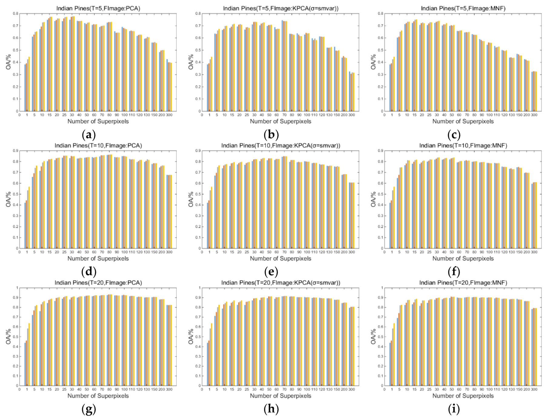
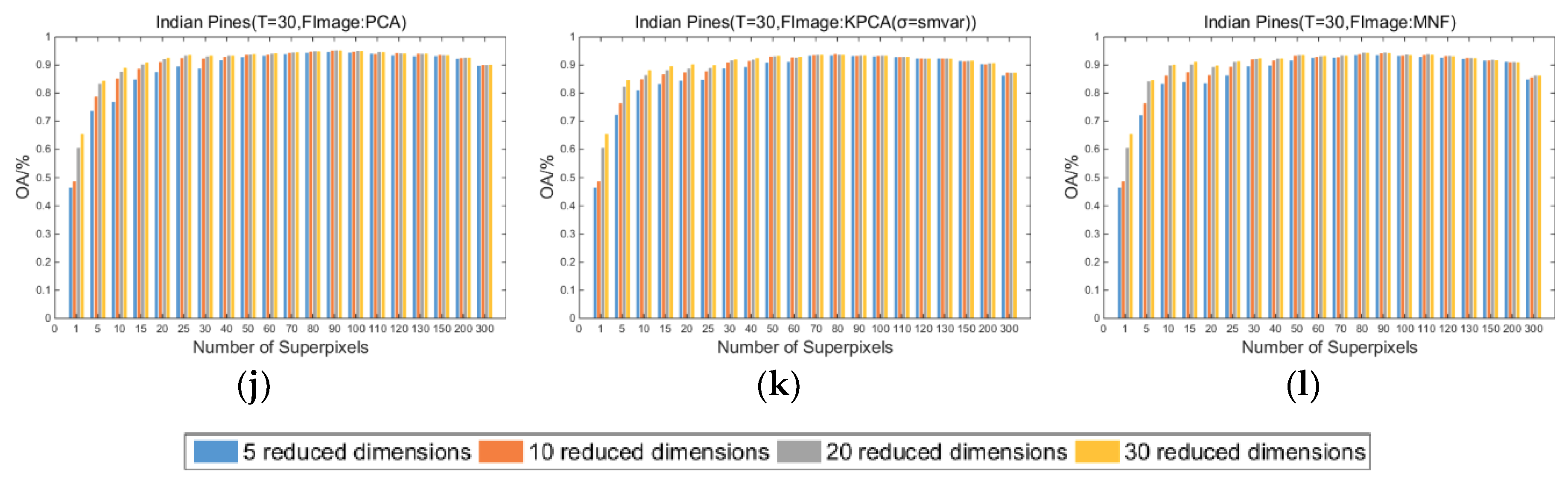
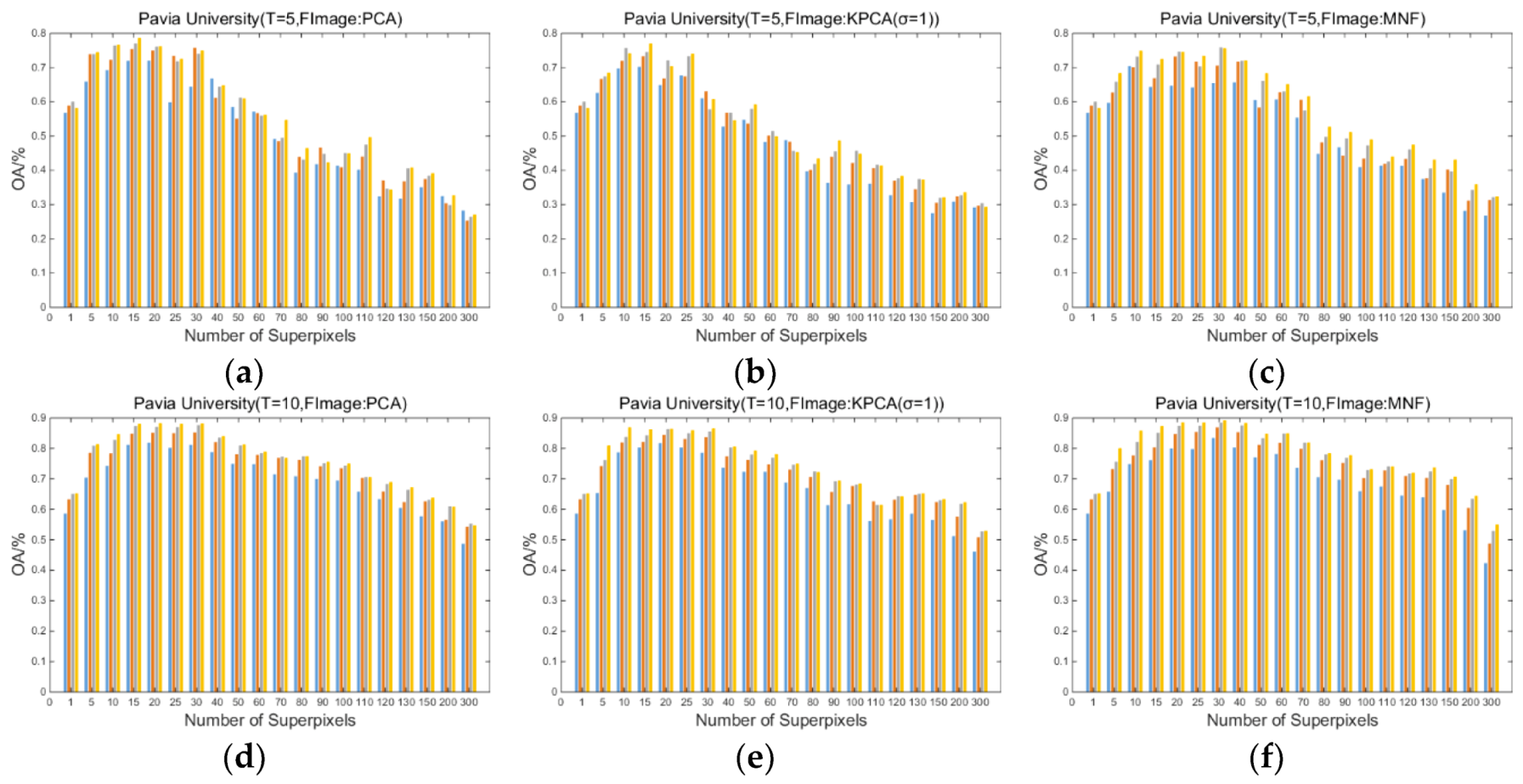
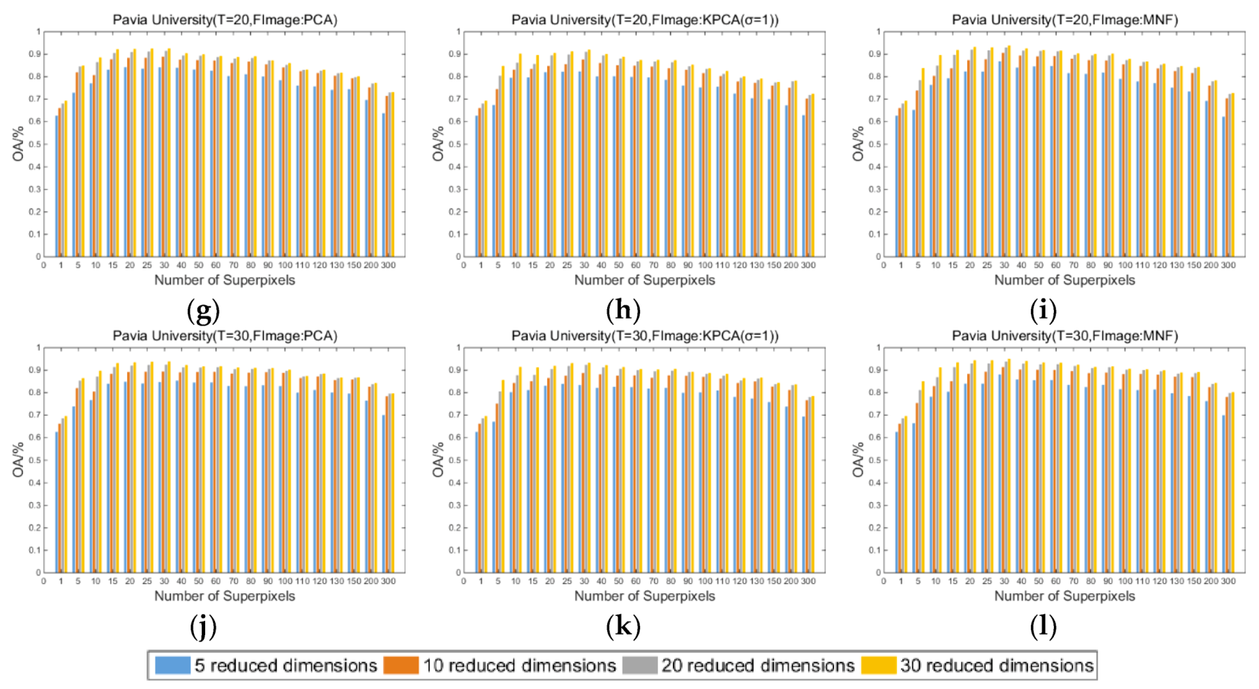
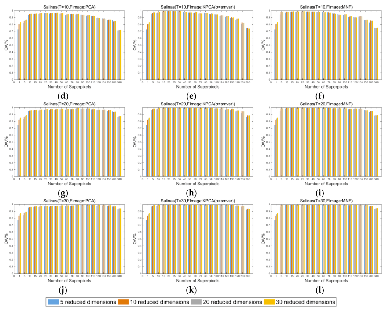
Figure 3, Figure 4, and Figure 5 show the influence of the number of superpixels on the overall classification accuracy (OA/%) of the proposed SuperKPCA method when the datasets are Indian Pines, Pavia University, and Salinas, respectively, where the number of superpixels is selected from . For each figure, the number of training samples is 5, 10, 20, and 30 from the first to the last row, and the blue, orange, gray, and red bars represent the OA when the reduced dimensions are 5, 10, 20, and 30, respectively. “FImage: PCA” indicates that the fundamental image used for segmentation is the first PC obtained by PCA. “FImage: KPCA (σ = smvar)” indicates that the fundamental image for segmentation is the first PC obtained by KPCA, and the parameter σ of the RBF kernel is determined by the formula when acquiring the first PC. Correspondingly, “FImage:KPCA(σ = 1)” indicates that the parameter σ of the RBF kernel is equal to 1 when acquiring the first PC. “FImage: MNF” indicates that the fundamental image used for segmentation is the first PC obtained by MNF. Note that when dimensionality reduction is performed after the segmentation is completed, the values of σ are all determined by the formula in all experiments in this study.
(1) As the number of superpixels increases, the OAs of the three datasets tend to rise first and then decrease. Moreover, by setting a suitable number of superpixels, the classification accuracy is usually higher than that when the number of superpixels is 1 (no superpixel segmentation), which indicates that the superpixel-based KPCA is more efficient than traditional global KPCA.
(2) As the training samples increase, the difference in the OAs obtained at different superpixel numbers decreases. This decrease suggests that when there are enough training samples, a similarly high classification accuracy can be obtained by using a plurality of different superpixel numbers, which is more evident in the Indian Pines and Salinas datasets.
(3) In the Indian Pines and Salinas datasets, when superpixel segmentation is not performed, the difference in the OAs obtained by different reduced dimensions is greater than the difference in the OAs obtained when the appropriate number of superpixels is set. This finding shows that in these two datasets, when the appropriate number of superpixels is set, a small number of reduced dimensions can obtain good overall classification accuracy. However, the situation is different in the Pavia University dataset; when the number of training samples is 5, the change in the OA exhibits no obvious trend with an increase in the reduced dimension. When the number of training samples is 10, 20, and 30, the OA shows an increasing trend with the increase in the reduced dimension, which is different from the performance of the OA in the other two datasets, where OAs with fewer dimensions are essentially the same as OAs with more dimensions. This result may be because the texture features of the Pavia University dataset are more complex than the Indian Pines and Salinas datasets (see the classification maps below). That is, even if superpixel segmentation is used, the useful information is less concentrated in the first few PCs than in the other two datasets.
(4) When the fundamental image used for segmentation is the first PC obtained by PCA, for Indian Pines, Pavia University, and Salinas images, when the number of training samples is 5, the optimal number of superpixels is 30, 15, and 25, respectively; when the number of training samples is 10, the optimal number of superpixels is 80, 20, and 40, respectively; when the number of training samples is 20, the optimal number of superpixels is 80, 30, and 80, respectively; when the number of training samples is 30, the optimal number of superpixels is 90, 30, and 80, respectively. The optimal reduced dimension for all three datasets is 30 when the fundamental image used for segmentation is the first PC obtained by PCA, except when the number of training samples is 20 and 30, the optimal reduced dimension for Indian Pines is 20. When the fundamental image used for segmentation is the first PC obtained by KPCA or MNF, most of the optimal reduced dimensions are also 30. This finding suggests that although the subsequent kernel PCs may contain noise, the information in these kernel PCs still contributes to the improvement in classification accuracy.
(5) When the fundamental image is the first PC obtained by PCA or MNF, the OAs of Indian Pines and Pavia University images are roughly similar to, or smaller than, the OAs obtained by the first PC of PCA. However, when the fundamental image is the first PC obtained by KPCA or MNF, the OAs of the Salinas image are significantly higher than those of OAs obtained based on the first PC of PCA. This result is especially true when the number of training samples is small, such as 5 and 10, which at least indicates that it is not always possible to obtain an optimal segmentation result by using the first PC obtained by PCA as the fundamental image when performing segmentation. This finding will be further analyzed in the later sections.
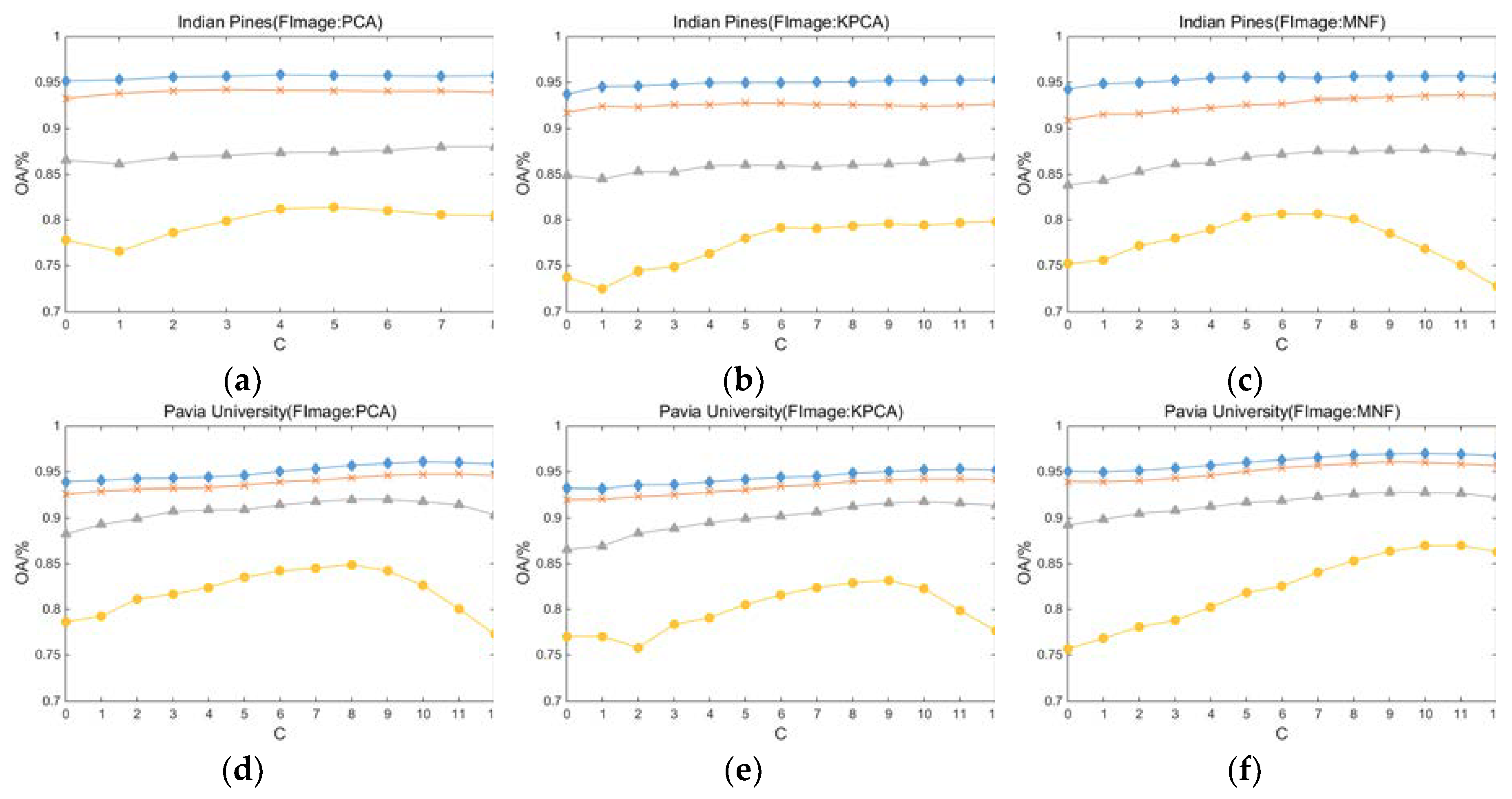
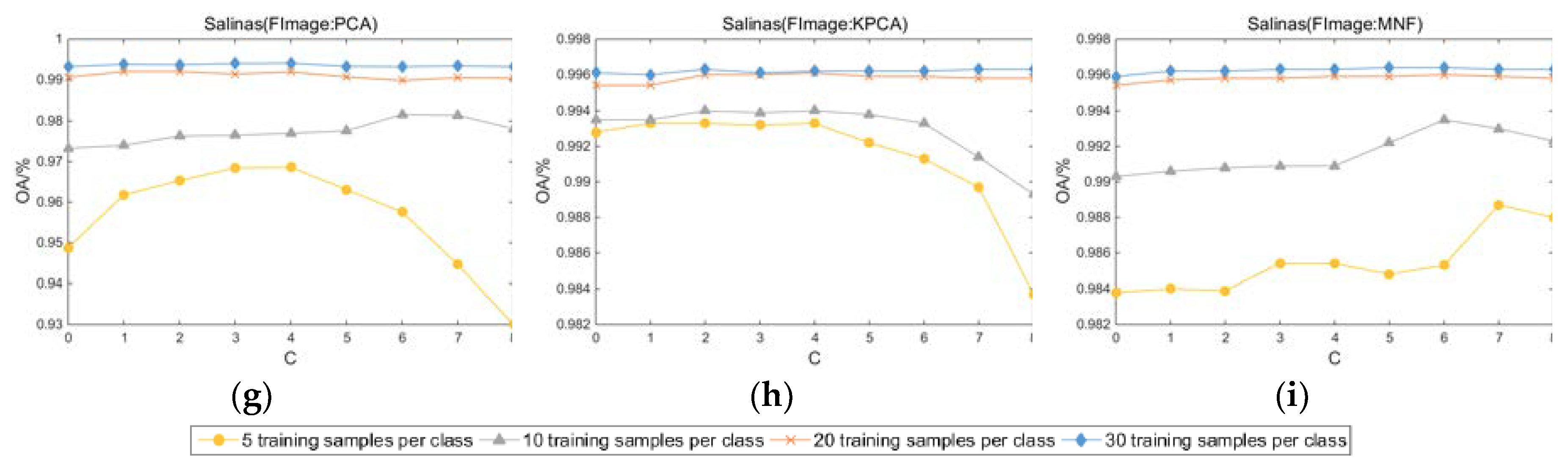
3.2.2. Analysis of the Impact of the Segmentation Scale
Based on the above experimental results, the optimal number of superpixels and reduced dimensions for the three datasets under different training sample numbers and fundamental images can be obtained. Notably, in most cases, the optimal reduced dimension is 30, but in a few cases, the optimal reduced dimension is 20 or even 5. Since there is a large difference in the number of superpixels when performing multiscale segmentation, for example, when the basic number of superpixels is 80 and the segmentation scale is 8, the number of superpixels includes 5, 7, 10, 14, 20, 28, 40, 56, 80, 113, 160, 226, 320, 452, 640, 905, and 1280. It can be seen from Figure 3 and Figure 4 that when the number of superpixels is small, more reduced dimensions are usually required to obtain higher classification accuracy. Therefore, in the following experiments, the reduced dimensions are all set to 30. The number of superpixels is the optimal number obtained in the previous experiments.
Setting the segmentation scale to 12 and using Equation (1), the OAs of the three datasets at different fundamental images and segmentation scales are obtained. The results are shown in Figure 6. Notably, the segmentation scale for the Salinas dataset is 8, and when the fundamental image is the first PC obtained by PCA, the segmentation scale for the Indian Pines dataset is also 8. It should also be noted that when the number of superpixels obtained by Equation (1) is less than 1, the number of superpixels is set to 1; that is, no superpixel segmentation is performed on the image.
From these results, the following conclusions can be drawn: (1) by fusing the classification results of multiscale segmentation, usually higher classification accuracy can be obtained; (2) when there are fewer training samples, such as training samples of 5 or 10, the use of multiscale fusion strategy can further increase the classification accuracy. Taking Figure 6a,d,g, for example, after setting the optimal segmentation scale, when the number of training samples is 5, the OA of the Indian Pines, Pavia University, and Salinas datasets increased by 4.62%, 7.99%, and 2.09%, respectively; when the number of training samples is 30, the overall accuracies are increased by 0.68%, 2.32%, and 0.10%, respectively. Another noteworthy phenomenon is that after setting the optimal segmentation scale, the improvement in OA is more obvious in the Pavia University dataset, and a larger c is usually required to obtain the optimal OA. As mentioned by Jiang et al. in [33], the texture features in the Pavia University dataset are more complex, making it more difficult for a single segmentation scale to accurately utilize its rich spatial information. At the same time, compared to the other two datasets, the Pavia University dataset requires more segmentation scales to accurately obtain spatial information for different sizes of objects.
3.3. Fusion of Multiscale Classification Results Based on Different Fundamental Images
To demonstrate the effectiveness of fusing multiscale classification results based on different fundamental images, both the classification accuracies of the fused results obtained based on the three different fundamental images and the classification accuracy after fusing all the multiscale classification results are shown in Table 2 (the number of training samples is 5). This study does not recombine the results of the three fused results. In contrast, based on the three different fundamental images, the study first separately performs multiscale segmentation, then performs dimensionality reduction and classification separately, and finally fuses all classification results. Here, the classification accuracies of the three fused results based on different fundamental images are shown to illustrate the difference in classification accuracy of multiscale fusion results based on different fundamental images. The PCA, KPCA, and MNF in Table 2 represent the classification accuracy of the fused results based on the first PC obtained by PCA, KPCA, and MNF, respectively, and 3M represents the classification accuracy after fusing all multiscale classification results. Since 10 different sets of training samples were selected for this study, Table 2 shows the classification results based on different fundamental images under a certain set of training samples.
As shown in Table 2, for each dataset, three different multiscale fusion results based on three different fundamental images have different classification accuracies in each category, and no fusion result can obtain the best classification accuracy in every category. However, when all multiscale classification results are fused, although the classification accuracy in each category is not all optimal, the OA, AA, and Kappa are higher than that in multiscale classification results based on a specific fundamental image. This result shows that different fundamental images represent the different main information of hyperspectral images, and for hyperspectral classification, it is an effective and trustworthy choice to fuse all multiscale classification results based on different fundamental images.
4. Discussion
4.1. Comparison with the State-of-the-art Approaches
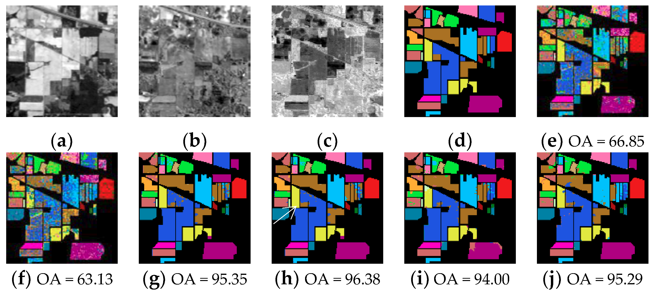
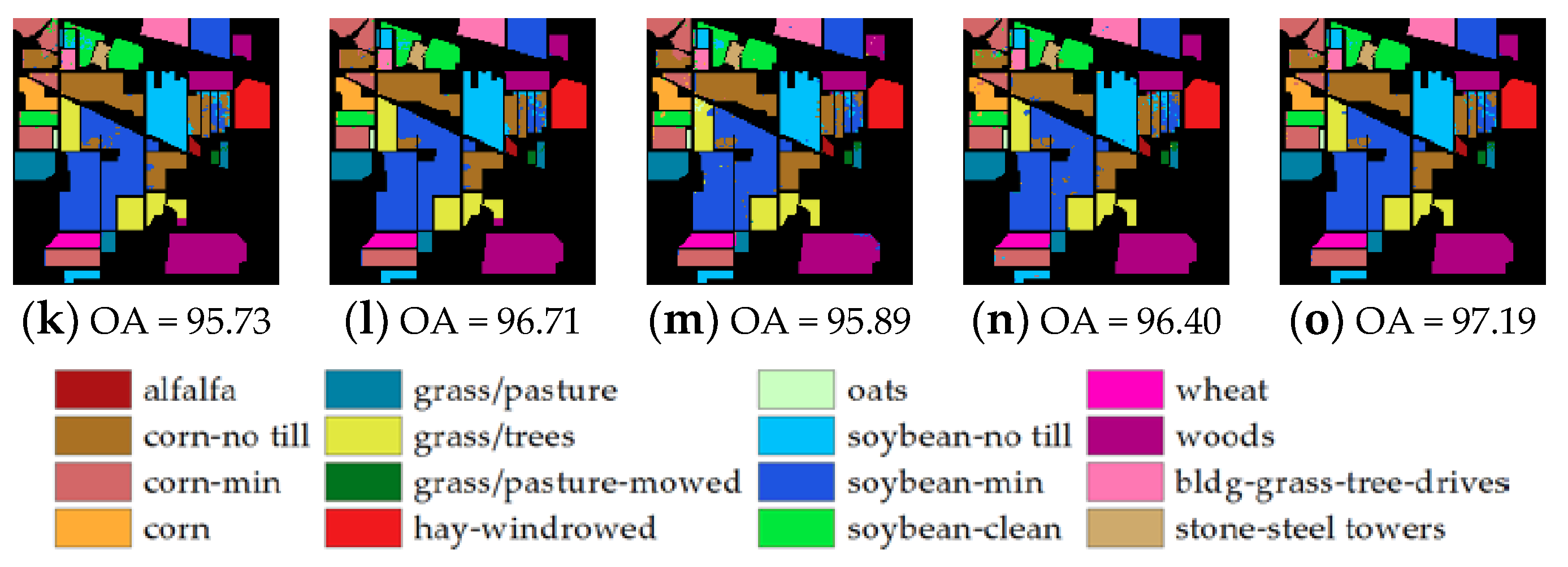
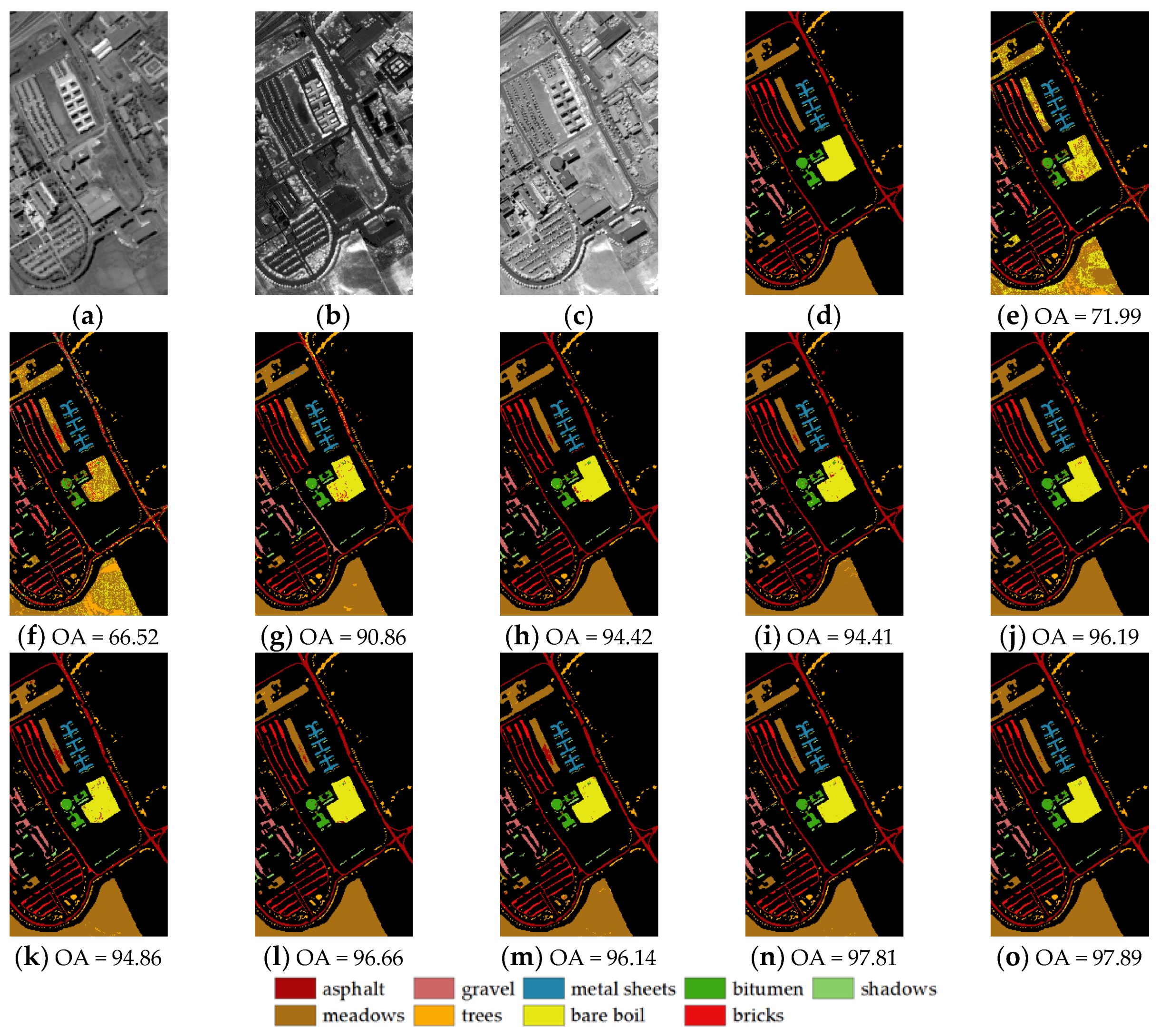
The classification maps of the three public datasets obtained by the proposed SuperKPCA and MSuperKPCA methods, as well as the methods used for comparison, are shown in Figure 7, Figure 8 and Figure 9. Here, only the classification maps obtained when the number of training samples is 30 are shown. Similar to the previous section, since this study selected 10 different training samples, Figure 7, Figure 8 and Figure 9 show the classification maps obtained under one set of training samples. SPCA(g) and MSPCA(k) represent the classification maps obtained by SuperPCA and MSuperPCA proposed in the previous study [33], respectively. Notably, the fundamental images used by these two methods are the first PCs obtained by PCA. When obtaining the classification maps of (g) and (k), the optimal number of superpixels is selected experimentally from the 20 candidate superpixels given above, and the optimal segmentation scale is also selected from 0 to 12 by experiments (for the Indian Pines and Pavia University datasets, the optimal segmentation scale is selected from 0 to 8 by experiments to ensure experimental consistency.). All of the superpixel-based classification maps shown in Figure 7, Figure 8 and Figure 9 are based on the optimal number of superpixels and segmentation scales obtained.
First, it can be seen from these classification maps that the superpixel-based dimensionality reduction method can greatly improve the classification accuracy compared to global PCA (e) and global KPCA (f). Second, the method based on multiscale segmentation (k–n) can further improve the classification accuracy compared to the method based on single-scale segmentation (g–j). For these three datasets, when no superpixel segmentation is performed, the classification accuracy obtained by KPCA (f) is lower than that obtained by PCA (e); however, when superpixel segmentation is performed, and the first PC after PCA is used as the fundamental image, the classification accuracy obtained by KPCA (h,l) is better than that obtained by PCA (g,k). This finding shows that in this experiment, when superpixel segmentation is performed, compared with PCA, KPCA can obtain better dimensionality reduction results due to its powerful ability in the field of nonlinear feature extraction.
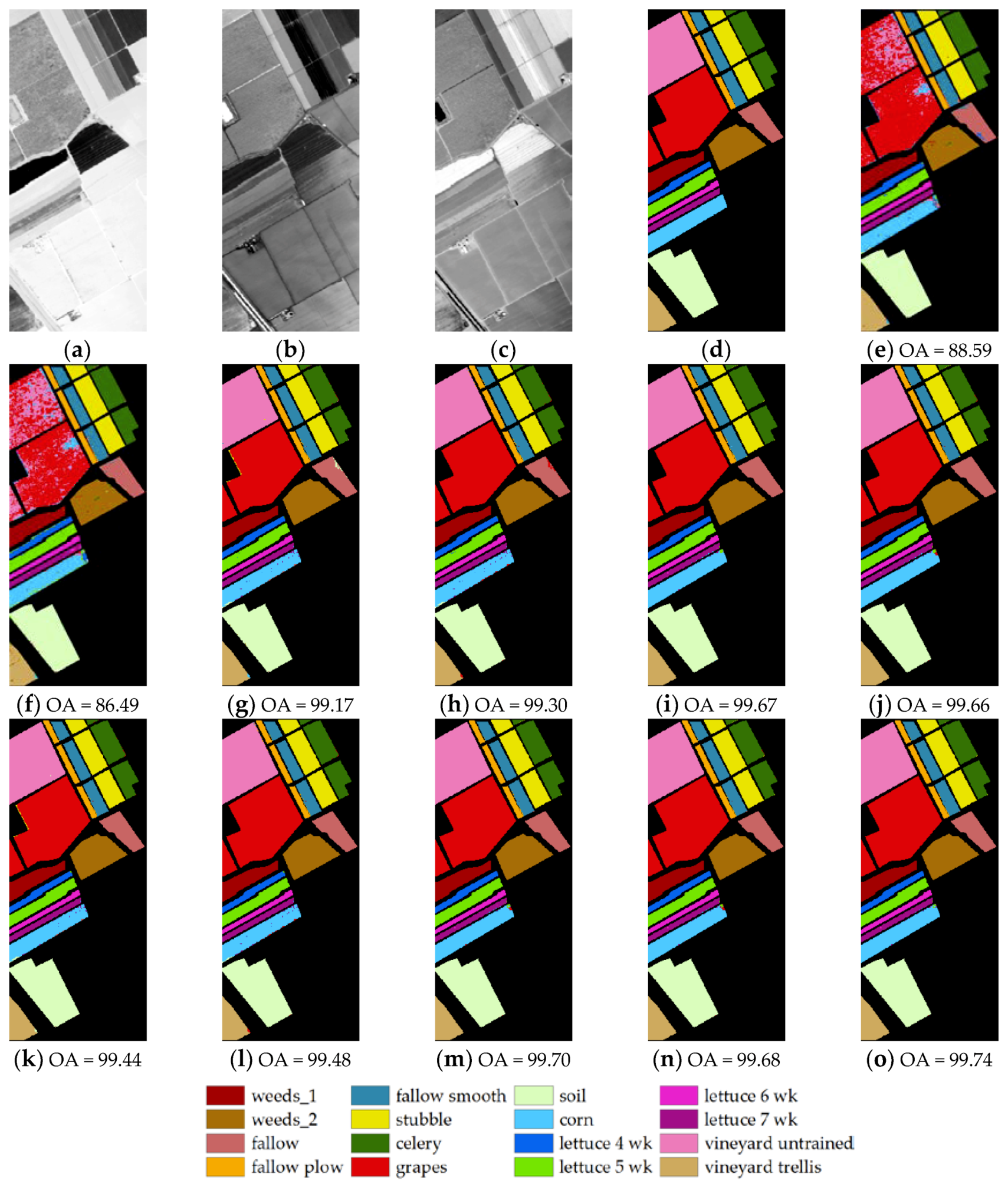
Moreover, by observing the parts indicated by the white arrows in each (h) classification map in Figure 7, Figure 8 and Figure 9, it can be seen that when the first PC after PCA is used as the fundamental image for segmentation, regardless of whether the method used for dimensionality reduction is PCA or KPCA, and whether multiscale segmentation is performed, there are classification errors in the parts indicated by the white arrows (g,h,k,l). However, when the first PC obtained by KPCA or MNF is used as the fundamental image, the parts indicated by the white arrows can be correctly classified (i,j,m,n). This result indicates that at least in this experiment, although using the first PC obtained by KPCA or MNF as the fundamental image for segmentation does not always achieve the best OA, it can perform better in a particular category.
However, this finding is not always the case. For example, in the (h) classification map in Figure 9, when the first PC after PCA is used as the fundamental image, the part indicated by the blue arrow has no classification error. However, when the dimensionality reduction is performed based on the first PC of KPCA or MNF, there is a classification error in the portion indicated by the blue arrow. This error further leads to classification errors in the same region in the final fused classification map. Nevertheless, after fusing the multiscale classification results based on different first PCs, the three datasets all show the best OAs (o). This finding indicates that in this experiment, the dimensionality reduction results obtained based on different first PCs are complementary, and the overall classification performance can be further improved by fusing the multiscale classification results obtained based on different first PCs.
To further illustrate the effectiveness of the proposed method, the OA obtained by the proposed method on the three datasets when the training samples T are 5, 10, 20, and 30 are shown in Table 3. It should be noted that all OAs are the average OA obtained using the 10 sets of random training samples disclosed in the previous study [33], and the process of selecting the optimal number of superpixels and the segmentation scale is the same as above when obtaining the OA of SuperPCA and MSuperPCA. The specific meaning of each method in the table is also consistent with the previous section. The global column in the table indicates the OA obtained without superpixel segmentation, and the single-scale and multiscale columns in the table represent the OA obtained by single-scale superpixel segmentation and multiscale superpixel segmentation, respectively.
To facilitate comparison and observation, the optimal OA of the three datasets under different numbers of training samples is bolded. For PCA and KPCA, Table 3 shows the optimal OA obtained when the reduced dimensions are set to 5, 10, 20, and 30, respectively. For the other methods, Table 3 shows the OA obtained when the reduced dimension is set to 30. When the number of training samples is 20 and 30, for the Pavia University dataset, the OA corresponding to 3-MSKPCA is the OA obtained by fusing the multiscale classification results obtained based on the first PCs of PCA and MNF.
The following conclusions can be drawn from Table 3:
(1) When no superpixel segmentation is performed, KPCA does not perform as well as PCA in all three datasets in most cases; however, when the first PC of PCA is used as the fundamental image, the performance of KPCA (P-SKPCA) is generally better than that of PCA (SPCA) when based on a single segmentation scale. For the Indian Pines, Pavia University, and Salinas datasets, the classification accuracy obtained by P-SKPCA can be increased by 0.06%–0.74%, 2.64%–4.23%, and 0.10%–0.41%, respectively, when compared with SPCA. This increase again proves that after using superpixel segmentation, KPCA can make better use of the nonlinear features that are widely present in hyperspectral images, thus showing better performance than PCA, and this advantage is most evident in the Pavia University dataset. This is mainly due to the fact that the texture features of the Pavia University dataset are more complex than the other two datasets. Therefore, the results obtained by nonlinear dimensionality reduction are more discriminating than those obtained by linear dimensionality reduction. When based on multiscale segmentation and using the first PC of PCA as the fundamental image, KPCA (P-MSKPCA) also outperforms PCA (MSPCA) in more cases.
(2) When using the first PC of KPCA or MNF as the fundamental image, whether based on a single segmentation scale or multiple segmentation scales, KPCA (K-SKPCA, M-SKPCA, K-MSKPCA, M-MSKPCA) does not perform as well as PCA (SPCA, MSPCA) in the Indian Pines dataset. However, KPCA performs generally better than PCA in the Pavia University and Salinas datasets, especially when based on a single segmentation scale. Moreover, in the Salinas dataset, KPCA’s performance based on a single segmentation scale (K-SKPCA, M-SKPCA) is even better than that of PCA after multiscale segmentation (MSPCA). By observing the performance of the proposed method based on single-scale segmentation and multiscale segmentation, in general, the fundamental image most suitable for the Indian Pines dataset is the first PC of PCA, the fundamental image most suitable for the Pavia University dataset is the first PC of MNF, and the fundamental image most suitable for the Salinas dataset is the first PC of KPCA. These results suggest that when performing superpixel segmentation, using the first PC of PCA as the fundamental image does not always achieve optimal dimensionality reduction results, and the most appropriate fundamental image needs to be determined on a case-by-case basis. For the Indian Pines, Pavia University, and Salinas datasets, when the most suitable fundamental image is selected, the classification accuracy obtained by SKPCA can be increased by 0.06%–0.74%, 3.88%–4.37%, and 0.39%–4.85%, respectively, when compared with SPCA; the classification accuracy obtained by MSKPCA can be increased by 0.66%–3.04%, 1.26%–3.20%, and 0.29%–2.54%, respectively, when compared with MSPCA.
(3) By observing the last column in Table 3, it can be found that except for the OA of the Pavia University dataset when the number of training samples is 20, all the OAs obtained by fusing multiscale classification results based on different fundamental images are higher than those obtained based only on one fundamental image. For the Indian Pines, Pavia University, and Salinas datasets, except for the OA of the Pavia University dataset when the number of training samples is 20, the classification accuracy obtained by 3-MSKPCA can be increased by 0.54%–2.68%, 0.12%–1.10%, and 0.01%–0.08%, respectively, when compared with MSKPCA (based on the most suitable fundamental image). This again shows that the dimensionality reduction results obtained based on different first PCs are complementary, and the overall classification performance can be further improved by fusing the multiscale classification results obtained based on different first PCs. Since the classification accuracy obtained by MSPCA is already high enough in the Salina dataset, the improvement of classification accuracy by 3-MSKPCA is not obvious in this dataset.
The above conclusions demonstrate the effectiveness of the proposed method once again.
4.2. Running Times
Table 4 reports the time required for the proposed method when performing dimensionality reduction. Since both PCA and KPCA are unsupervised dimensionality reduction methods, the time required for the proposed method is independent of the number of training samples. For those methods based on superpixel segmentation, Table 4 reports the total time required for segmentation and dimensionality reduction. To facilitate comparison of the different methods, for the three datasets, the time required for each method when the number of superpixels is set to 30 is reported.
All approaches were tested on Matlab using an Intel(R) Core (TM) i5-2430M CPU with 2.40 GHz and a 4-GB memory personal computer with a Windows 10 platform, and the testing time was measured using a single-threaded Matlab process. Since the kernel parameter σ needs to be estimated, KPCA does not have an advantage in terms of runtime, whether superpixel segmentation is performed, but the time required for the proposed method is still within an acceptable range.
5. Conclusions
This study proposes a simple but effective unsupervised dimensionality reduction method based on SuperKPCA. Extensive experiments show that since superpixels can contain both spatial and spectral information of HSIs, the ability of KPCA to process nonlinear features can be greatly increased by performing KPCA on each superpixel. Moreover, whether based on single-scale segmentation or multiscale segmentation, the proposed method performs better than SuperPCA (by performing PCA on each superpixel) in most cases. For the Indian Pines, Pavia University, and Salinas datasets, when the most suitable fundamental image is selected, the classification accuracy obtained by SuperKPCA can be increased by 0.06%–0.74%, 3.88%–4.37%, and 0.39%–4.85%, respectively, when compared with SuperPCA; the classification accuracy obtained by MSuperKPCA (SuperKPCA based on multiscale) can be increased by 0.66%–3.04%, 1.26%–3.20%, and 0.29%–2.54%, respectively, when compared with MSuperPCA (SuperPCA based on multiscale). To explore whether the first PC obtained by PCA is the best fundamental image when performing superpixel segmentation, the differences in the classification results of the proposed method when the fundamental images are the first PCs of PCA, KPCA, and MNF, respectively, are compared. Extensive experiments show that the optimal fundamental images corresponding to different hyperspectral images are different, and by fusing the dimensionality reduction results obtained based on different fundamental images (3-MSKPCA), the rich spatial information in HSIs can usually be further utilized, and the dimensionality reduction performance can usually be further improved. For the Indian Pines, Pavia University, and Salinas datasets, except for the classification accuracy of the Pavia University dataset when the number of training samples is 20, the classification accuracy obtained by 3-MSKPCA can be increased by 0.54%–2.68%, 0.12%–1.10%, and 0.01%–0.08%, respectively, when compared with MSuperKPCA (based on the most suitable fundamental image).
Since the proposed method is based on superpixels, how to determine the number of superpixels is a very important issue. If the number of superpixels is too large or too small, the rich spatial information in HSIs cannot be fully utilized. In this study, the optimal number of superpixels was selected experimentally from a set of candidate numbers. In the future work, how to narrow the range of candidate numbers, or how to automatically obtain the optimal number of superpixels, will be a major problem that needs to be solved.
Author Contributions
L.Z. proposed the methods, implemented the experiments, and drafted the manuscript. H.S. and J.S. reviewed and edited the manuscript. J.S. provided overall guidance to the project and obtained funding to support this research.
Funding
This research was supported by the Fundamental Research Funds for the Central Universities (No. XDJK2019B008). We would like to thank the editors and anonymous referees for their constructive comments.
Conflicts of Interest
The authors declare no conflict of interest. The funders had no role in the design of the study; in the collection, analyses, or interpretation of data; in the writing of the manuscript, or in the decision to publish the results.
References
- Li, W.; Feng, F.; Li, H.; Du, Q. Discriminant analysis-based dimension reduction for hyperspectral image classification: A survey of the most recent advances and an experimental comparison of different techniques. IEEE Geosci. Remote Sens. Mag. 2018, 6, 15–34. [Google Scholar] [CrossRef]
- Hughes, G. On the mean accuracy of statistical pattern recognizers. IEEE Trans. Inf. Theory 1968, 14, 55–63. [Google Scholar] [CrossRef]
- Pearson, K. LIII. On lines and planes of closest fit to systems of points in space. Lond. Edinb. Dublin Philos. Mag. J. Sci. 1901, 2, 559–572. [Google Scholar] [CrossRef]
- Bachmann, C.M.; Ainsworth, T.L.; Fusina, R.A. Exploiting manifold geometry in hyperspectral imagery. IEEE Trans. Geosci. Remote Sens. 2005, 43, 441–454. [Google Scholar] [CrossRef]
- Keshava, N.; Mustard, J.F. Spectral unmixing. IEEE Signal Process. Mag. 2002, 19, 44–57. [Google Scholar] [CrossRef]
- Scholz, M.; Kaplan, F.; Guy, C.L.; Kopka, J.; Selbig, J. Non-linear PCA: A missing data approach. Bioinformatics 2005, 21, 3887–3895. [Google Scholar] [CrossRef]
- Zhang, H.; Pedrycz, W.; Miao, D.; Wei, Z. From principal curves to granular principal curves. IEEE Trans. Cybern. 2014, 44, 748–760. [Google Scholar] [CrossRef]
- Lu, H.; Plataniotis, K.N.; Venetsanopoulos, A.N. A survey of multilinear subspace learning for tensor data. Pattern Recognit. 2011, 44, 1540–1551. [Google Scholar] [CrossRef]
- Schölkopf, B.; Smola, A.; Müller, K.-R. Nonlinear component analysis as a kernel eigenvalue problem. Neural Comput. 1998, 10, 1299–1319. [Google Scholar] [CrossRef]
- Filho, J.B.O.S.; Diniz, P.S.R. A fixed-point online kernel principal component extraction algorithm. IEEE Trans. Signal Process. 2017, 65, 6244–6259. [Google Scholar] [CrossRef]
- Filho, J.B.O.S.; Diniz, P.S.R. Improving KPCA online extraction by orthonormalization in the feature space. IEEE Trans. Neural Netw. Learn. Syst. 2018, 29, 1382–1387. [Google Scholar] [CrossRef] [PubMed]
- Washizawa, Y. Adaptive subset kernel principal component analysis for time-varying patterns. IEEE Trans. Neural Netw. Learn. Syst. 2012, 23, 1961–1973. [Google Scholar] [CrossRef] [PubMed]
- Gan, L.; Xia, J.; Du, P.; Chanussot, J. Multiple feature kernel sparse representation classifier for hyperspectral imagery. IEEE Trans. Geosci. Remote Sens. 2018, 56, 5343–5356. [Google Scholar] [CrossRef]
- Honeine, P. Online kernel principal component analysis: A reduced-order model. IEEE Trans. Pattern Anal. Mach. Intell. 2012, 34, 1814–1826. [Google Scholar] [CrossRef] [PubMed]
- Papaioannou, A.; Zafeiriou, S. Principal component analysis with complex kernel: The widely linear Model. IEEE Trans. Neural Netw. Learn. Syst. 2014, 25, 1719–1726. [Google Scholar] [CrossRef]
- Chakour, C.; Benyounes, A.; Boudiaf, M. Diagnosis of uncertain nonlinear systems using interval kernel principal components analysis: Application to a weather station. ISA Trans. 2018, 83, 126–141. [Google Scholar] [CrossRef]
- Jaffel, I.; Taouali, O.; Harkat, M.F.; Messaoud, H. Moving window KPCA with reduced complexity for nonlinear dynamic process monitoring. I|Sa Trans. 2016, 64, 184–192. [Google Scholar] [CrossRef]
- Jia, S.; Wu, K.; Zhu, J.; Jia, X. Spectral–spatial gabor surface feature fusion Approach for hyperspectral imagery classification. IEEE Trans. Geosci. Remote Sens. 2019, 57, 1142–1154. [Google Scholar] [CrossRef]
- Guo, Y.; Jiao, L.; Wang, S.; Wang, S.; Liu, F.; Hua, W. Fuzzy superpixels for polarimetric SAR images classification. IEEE Trans. Fuzzy Syst. 2018, 26, 2846–2860. [Google Scholar] [CrossRef]
- Berveglieri, A.; Imai, N.N.; Tommaselli, A.M.G.; Casagrande, B.; Honkavaara, E. Successional stages and their evolution in tropical forests using multi-temporal photogrammetric surface models and superpixels. ISPRS J. Photogramm. Remote Sens. 2018, 146, 548–558. [Google Scholar] [CrossRef]
- Huang, X.; Chen, H.; Gong, J. Angular difference feature extraction for urban scene classification using ZY-3 multi-angle high-resolution satellite imagery. ISPRS J. Photogramm. Remote Sens. 2018, 135, 127–141. [Google Scholar] [CrossRef]
- Jia, S.; Deng, B.; Zhu, J.; Jia, X.; Li, Q. Local binary pattern-based hyperspectral image classification with superpixel guidance. IEEE Trans. Geosci. Remote Sens. 2018, 56, 749–759. [Google Scholar] [CrossRef]
- Belgiu, M.; Csillik, O. Sentinel-2 cropland mapping using pixel-based and object-based time-weighted dynamic time warping analysis. Remote Sens. Environ. 2018, 204, 509–523. [Google Scholar] [CrossRef]
- Zhang, C.; Sargent, I.; Pan, X.; Li, H.; Gardiner, A.; Hare, J.; Atkinson, P.M. Joint deep learning for land cover and land use classification. Remote Sens. Environ. 2019, 221, 173–187. [Google Scholar] [CrossRef]
- Zhang, C.; Sargent, I.; Pan, X.; Li, H.; Gardiner, A.; Hare, J.; Atkinson, P.M. An object-based convolutional neural network (OCNN) for urban land use classification. Remote Sens. Environ. 2018, 216, 57–70. [Google Scholar] [CrossRef] [Green Version]
- Massey, R.; Sankey, T.T.; Yadav, K.; Congalton, R.G.; Tilton, J.C. Integrating cloud-based workflows in continental-scale cropland extent classification. Remote Sens. Environ. 2018, 219, 162–179. [Google Scholar] [CrossRef]
- Fauvel, M.; Tarabalka, Y.; Benediktsson, J.A.; Chanussot, J.; Tilton, J.C. Advances in spectral-spatial classification of hyperspectral images. Proc. IEEE 2013, 101, 652–675. [Google Scholar] [CrossRef]
- Lv, X.; Ming, D.; Lu, T.; Zhou, K.; Wang, M.; Bao, H. A new method for region-based majority voting CNNs for very high resolution image classification. Remote Sens. 2018, 10, 1946. [Google Scholar] [CrossRef]
- Feng, J.; Wang, L.; Yu, H.; Jiao, L.; Zhang, X. Divide-and-conquer dual-architecture convolutional neural network for classification of hyperspectral images. Remote Sens. 2019, 11, 484. [Google Scholar] [CrossRef]
- Zhang, S.; Li, S.; Fu, W.; Fang, L. Multiscale superpixel-based sparse representation for hyperspectral Image classification. Remote Sens. 2017, 9, 139. [Google Scholar] [CrossRef]
- Cui, B.; Xie, X.; Ma, X.; Ren, G.; Ma, Y. Superpixel-based extended random walker for hyperspectral image classification. IEEE Trans. Geosci. Remote Sens. 2018, 56, 3233–3243. [Google Scholar] [CrossRef]
- Jin, X.; Gu, Y. Superpixel-based intrinsic image decomposition of hyperspectral images. IEEE Trans. Geosci. Remote Sens. 2017, 55, 4285–4295. [Google Scholar] [CrossRef]
- Jiang, J.; Ma, J.; Chen, C.; Wang, Z.; Cai, Z.; Wang, L. Super PCA: A superpixelwise PCA approach for unsupervised feature extraction of hyperspectral imagery. IEEE Trans. Geosci. Remote Sens. 2018, 56, 4581–4593. [Google Scholar] [CrossRef]
- Mountrakis, G.; Im, J.; Ogole, C. Support vector machines in remote sensing: A review. ISPRS J. Photogramm. Remote Sens. 2011, 66, 247–259. [Google Scholar] [CrossRef]
- Mohammadimanesh, F.; Salehi, B.; Mahdianpari, M.; Motagh, M.; Brisco, B. An efficient feature optimization for wetland mapping by synergistic use of SAR intensity, interferometry, and polarimetry data. Int. J. Appl. Earth Obs. Geoinf. 2018, 73, 450–462. [Google Scholar] [CrossRef]
- Green, A.A.; Berman, M.; Switzer, P.; Craig, M.D. A transformation for ordering multispectral data in terms of image quality with implications for noise removal. IEEE Trans. Geosci. Remote Sens. 1988, 26, 65–74. [Google Scholar] [CrossRef] [Green Version]
- Achanta, R.; Shaji, A.; Smith, K.; Lucchi, A.; Fua, P.; Süsstrunk, S. SLIC superpixels compared to state-of-the-art superpixel methods. IEEE Trans. Pattern Anal. Mach. Intell. 2012, 34, 2274–2282. [Google Scholar] [CrossRef] [PubMed]
- Vincent, L.; Soille, P. Watersheds in digital spaces: An efficient algorithm based on immersion simulations. IEEE Trans. Pattern Anal. Mach. Intell. 1991, 13, 583–598. [Google Scholar] [CrossRef]
- Comaniciu, D.; Meer, P. Mean shift: A robust approach toward feature space analysis. IEEE Trans. Pattern Anal. Mach. Intell. 2002, 24, 603–619. [Google Scholar] [CrossRef]
- Liu, M.; Tuzel, O.; Ramalingam, S.; Chellappa, R. Entropy rate superpixel segmentation. In Proceedings of the CVPR 2011, Colorado Springs, CO, USA, 20–25 June 2011; pp. 2097–2104. [Google Scholar]
- Dong, X.; Shen, J.; Shao, L.; Gool, L.V. Sub-markov random walk for image segmentation. IEEE Trans. Image Process. 2016, 25, 516–527. [Google Scholar] [CrossRef]
- Felzenszwalb, P.F.; Huttenlocher, D.P. Efficient graph-based image segmentation. Int. J. Comput. Vis. 2004, 59, 167–181. [Google Scholar] [CrossRef]
- Jianbo, S.; Malik, J. Normalized cuts and image segmentation. IEEE Trans. Pattern Anal. Mach. Intell. 2000, 22, 888–905. [Google Scholar] [CrossRef]
- Liang, X.; Xu, C.; Shen, X.; Yang, J.; Tang, J.; Lin, L.; Yan, S. Human parsing with contextualized convolutional neural network. IEEE Trans. Pattern Anal. Mach. Intell. 2017, 39, 115–127. [Google Scholar] [CrossRef]
- He, Z.; Liu, L.; Zhou, S.; Shen, Y. Learning group-based sparse and low-rank representation for hyperspectral image classification. Pattern Recognit. 2016, 60, 1041–1056. [Google Scholar] [CrossRef]
- Cao, L.; Luo, F.; Chen, L.; Sheng, Y.; Wang, H.; Wang, C.; Ji, R. Weakly supervised vehicle detection in satellite images via multi-instance discriminative learning. Pattern Recognit. 2017, 64, 417–424. [Google Scholar] [CrossRef]
- Widjaja, D.; Varon, C.; Dorado, A.; Suykens, J.A.K.; Huffel, S.V. Application of kernel principal component analysis for single-lead-ECG-derived respiration. IEEE Trans. Biomed. Eng. 2012, 59, 1169–1176. [Google Scholar] [CrossRef]
- Xie, L.; Li, Z.; Zeng, J.; Kruger, U. Block adaptive kernel principal component analysis for nonlinear process monitoring. AIChE J. 2016, 62, 4334–4345. [Google Scholar] [CrossRef]
- Chang, C.-C.; Lin, C.-J. LIBSVM: A library for support vector machines. ACM Trans. Intell. Syst. Technol. 2011, 2, 1–27. [Google Scholar] [CrossRef]
Figure 1.
Schematic of SuperKPCA.

Figure 2.
Schematic illustration of the MSuperKPCA algorithm based on different fundamental images for HSI classification.
Figure 2.
Schematic illustration of the MSuperKPCA algorithm based on different fundamental images for HSI classification.

Figure 3.
Influences of the number of superpixels on the overall accuracy (OA) of the proposed superpixelwise kernel principal component analysis (SuperKPCA) method for the Indian Pines dataset, where ”T” represents the number of pixels of the training sample: (a,d,g,j) the fundamental image is obtained by principal component analysis (PCA); (b,e,h,k) the fundamental image is obtained by kernel PCA (KPCA), and the parameter σ of the radial basis function kernel is determined by the formula when acquiring the fundamental image; and (c,f,I,l) the fundamental image is obtained by minimum noise fraction (MNF).


Figure 4.
Influences of the number of superpixels on the overall accuracy (OA) of the proposed superpixelwise kernel principal component analysis (SuperKPCA) method for the Pavia University dataset, where ”T” represents the number of pixels of the training sample: (a,d,g,j) the fundamental image is obtained by principal component analysis (PCA); (b,e,h,k) the fundamental image is obtained by kernel KPCA (KPCA), and the parameter σ of the radial basis function kernel is equal to 1 when acquiring the fundamental image; and (c)(f)(i)(l) the fundamental image is obtained by minimum noise fraction (MNF).


Figure 5.
Influences of the number of superpixels on the overall accuracy (OA) of the proposed superpixelwise kernel principal component analysis (SuperKPCA) method for the Salinas dataset, where ”T” represents the number of pixels of the training sample: (a,d,g,j) the fundamental image is obtained by principal component analysis (PCA); (b,e,h,k) the fundamental image is obtained by kernel PCA (KPCA), and the parameter σ of the radial basis function kernel is determined by the formula when acquiring the fundamental image; and (c,f,I,l) the fundamental image is obtained by minimum noise fraction (MNF).


Figure 6.
Effects of segmentation scale on overall accuracy (OA): (a–c) Indian Pines; (d–f) Pavia University; and (g–i) Salinas.
Figure 6.
Effects of segmentation scale on overall accuracy (OA): (a–c) Indian Pines; (d–f) Pavia University; and (g–i) Salinas.


Figure 7.
Classification maps of the Indian Pines dataset: (a) first principal component (PC) obtained by principal component analysis (PCA); (b) first PC obtained by kernel PCA (KPCA); (c) first PC obtained by minimum noise fraction (MNF); (d) ground truth; (e) PCA; (f) KPCA; (g) superpixelwise PCA (SuperPCA, also SPCA); (h) superpixelwise KPCA (SuperKPCA, also SKPCA) based on the first PC obtained by PCA (P-SKPCA); (i) SKPCA based on the first PC obtained by KPCA (K-SKPCA); (j) SKPCA based on the first PC obtained by MNF (M-SKPCA); (k) multiscale segmentation-based SPCA (MSuperPCA, also MSPCA); (l) multiscale segmentation-based SKPCA (MSuperKPCA, also MSKPCA) based on the first PC obtained by PCA (P-MSKPCA); (m) MSKPCA based on the first PC obtained by KPCA (K-MSKPCA); (n) MSKPCA based on the first PC obtained by MNF (M-MSKPCA); and (o) the fusion of all multiscale classification results obtained by MSKPCA based on the three different fundamental images: the first PCs obtained by PCA, KPCA and MNF (3-MSKPCA).


Figure 8.
Classification maps of the Pavia University dataset: (a) first principal component (PC) obtained by principal component analysis (PCA); (b) first PC obtained by kernel PCA (KPCA); (c) first PC obtained by minimum noise fraction (MNF); (d) ground truth; (e) PCA; (f) KPCA; (g) superpixelwise PCA (SuperPCA, also SPCA); (h) superpixelwise KPCA (SuperKPCA, also SKPCA) based on the first PC obtained by PCA (P-SKPCA); (i) SKPCA based on the first PC obtained by KPCA (K-SKPCA); (j) SKPCA based on the first PC obtained by MNF (M-SKPCA); (k) multiscale segmentation-based SPCA (MSuperPCA, also MSPCA); (l) multiscale segmentation-based SKPCA (MSuperKPCA, also MSKPCA) based on the first PC obtained by PCA (P-MSKPCA); (m) MSKPCA based on the first PC obtained by KPCA (K-MSKPCA); (n) MSKPCA based on the first PC obtained by MNF (M-MSKPCA); and (o) the fusion of all multiscale classification results obtained by MSKPCA based on the fundamental images: the first PCs obtained by PCA and MNF.

Figure 9.
Classification maps of the Salinas dataset: (a) first principal component (PC) obtained by principal component analysis (PCA); (b) first PC obtained by kernel PCA (KPCA); (c) first PC obtained by minimum noise fraction (MNF); (d) ground truth; (e) PCA; (f) KPCA; (g) superpixelwise PCA (SuperPCA, also SPCA); (h) superpixelwise KPCA (SuperKPCA, also SKPCA) based on the first PC obtained by PCA (P-SKPCA); (i) SKPCA based on the first PC obtained by KPCA (K-SKPCA); (j) SKPCA based on the first PC obtained by MNF (M-SKPCA); (k) multiscale segmentation-based SPCA (MSuperPCA, also MSPCA); (l) multiscale segmentation-based SKPCA (MSuperKPCA, also MSKPCA) based on the first PC obtained by PCA (P-MSKPCA); (m) MSKPCA based on the first PC obtained by KPCA (K-MSKPCA); (n) MSKPCA based on the first PCs obtained by MNF (M-MSKPCA); and (o) the fusion of all multiscale classification results obtained by MSKPCA based on the three different fundamental images: the first PC obtained by PCA, KPCA and MNF (3-MSKPCA).


Table 1.
The sample size for each class in the three used datasets.
| Indian Pines | Pavia University | Salinas | ||||
|---|---|---|---|---|---|---|
| Class | Categories | Samples | Categories | Samples | Categories | Samples |
| 1 | alfalfa | 46 | asphalt | 6631 | weeds_1 | 2009 |
| 2 | corn-no till | 1428 | meadows | 18,649 | weeds_2 | 3726 |
| 3 | corn-min | 830 | gravel | 2099 | fallow | 1976 |
| 4 | corn | 237 | trees | 3064 | fallow plow | 1394 |
| 5 | grass or pasture | 483 | metal sheets | 1345 | fallow smooth | 2678 |
| 6 | grass or trees | 730 | bare boil | 5029 | stubble | 3959 |
| 7 | grass or pasture-mowed | 28 | bitumen | 1330 | celery | 3579 |
| 8 | hay-windrowed | 478 | bricks | 3682 | grapes | 11,271 |
| 9 | oats | 20 | shadows | 947 | soil | 6203 |
| 10 | soybean-no till | 972 | corn | 3278 | ||
| 11 | soybean-min | 2455 | lettuce 4 wk | 1068 | ||
| 12 | soybean-clean | 593 | lettuce 5 wk | 1927 | ||
| 13 | wheat | 205 | lettuce 6 wk | 916 | ||
| 14 | woods | 1265 | lettuce 7 wk | 1070 | ||
| 15 | buildings-grass-tree-drives | 386 | vineyard untrained | 7268 | ||
| 16 | stone-steel towers | 93 | vineyard trellis | 1807 | ||
| total | 10,249 | total | 42,776 | total | 54,129 | |
Table 2.
Classification accuracy after multiscale fusion when the number of training samples is 5.
| Indian Pines | Pavia University | Salinas | ||||||||||
|---|---|---|---|---|---|---|---|---|---|---|---|---|
| Class | PCA | KPCA | MNF | 3M 1 | PCA | KPCA | MNF | 3M | PCA | KPCA | MNF | 3M |
| 1 | 97.56 | 97.56 | 97.56 | 97.56 | 75.42 | 76.37 | 84.38 | 83.76 | 100.00 | 100.00 | 100.00 | 100.00 |
| 2 | 77.30 | 68.59 | 84.68 | 72.24 | 94.07 | 89.83 | 91.61 | 95.64 | 100.00 | 100.00 | 100.00 | 100.00 |
| 3 | 86.06 | 83.88 | 79.27 | 86.91 | 79.94 | 88.73 | 74.74 | 83.62 | 100.00 | 100.00 | 100.00 | 100.00 |
| 4 | 97.84 | 91.38 | 93.97 | 94.83 | 89.74 | 83.39 | 94.08 | 94.15 | 99.64 | 99.78 | 99.86 | 99.86 |
| 5 | 83.89 | 81.59 | 83.26 | 83.47 | 99.25 | 99.33 | 99.40 | 99.40 | 97.31 | 97.49 | 98.88 | 97.83 |
| 6 | 99.59 | 76.28 | 74.90 | 84.00 | 87.52 | 64.77 | 83.48 | 86.62 | 99.87 | 99.97 | 99.87 | 99.92 |
| 7 | 95.65 | 100.00 | 100.00 | 100.00 | 94.04 | 93.21 | 97.06 | 96.00 | 99.92 | 99.72 | 99.50 | 99.75 |
| 8 | 100.00 | 100.00 | 100.00 | 100.00 | 90.21 | 92.30 | 78.68 | 92.44 | 97.89 | 100.00 | 100.00 | 100.00 |
| 9 | 100.00 | 100.00 | 100.00 | 100.00 | 79.94 | 84.39 | 86.73 | 88.96 | 99.65 | 99.97 | 99.97 | 99.98 |
| 10 | 84.07 | 85.11 | 85.01 | 85.63 | 98.81 | 98.96 | 97.04 | 99.08 | ||||
| 11 | 82.16 | 90.78 | 72.45 | 91.35 | 96.14 | 95.39 | 100.00 | 98.12 | ||||
| 12 | 93.54 | 72.79 | 35.20 | 88.61 | 86.73 | 99.95 | 100.00 | 98.23 | ||||
| 13 | 99.50 | 99.50 | 99.50 | 99.50 | 98.24 | 97.04 | 97.15 | 97.69 | ||||
| 14 | 80.95 | 99.76 | 99.92 | 100.00 | 98.12 | 93.05 | 93.99 | 95.77 | ||||
| 15 | 76.64 | 79.53 | 75.59 | 77.17 | 95.75 | 99.53 | 99.90 | 99.93 | ||||
| 16 | 95.45 | 97.73 | 86.36 | 94.32 | 99.06 | 100.00 | 100.00 | 99.89 | ||||
| OA(%) | 85.37 | 85.50 | 80.59 | 87.98 | 88.92 | 84.77 | 88.08 | 91.75 | 98.07 | 99.44 | 99.54 | 99.57 |
| AA(%) | 90.64 | 89.03 | 85.48 | 90.97 | 87.79 | 85.81 | 87.80 | 91.18 | 97.95 | 98.80 | 99.13 | 99.13 |
| Kappa | 0.8340 | 0.8344 | 0.7802 | 0.8629 | 0.8539 | 0.7987 | 0.8433 | 0.8908 | 0.9785 | 0.9944 | 0.9948 | 0.9953 |
1 The classification accuracy after fusing all multiscale classification results based on the three different fundamental images: the first principal components obtained by principal component analysis (PCA), kernel PCA (KPCA) and minimum noise fraction (MNF).
Table 3.
The OA obtained based on different dimensionality reduction methods when the training samples T are 5, 10, 20, and 30, respectively.
Table 3.
The OA obtained based on different dimensionality reduction methods when the training samples T are 5, 10, 20, and 30, respectively.
| T | Global | Single-scale | Multiscale | |||||||||
|---|---|---|---|---|---|---|---|---|---|---|---|---|
| PCA | K PCA | S PCA | P-SKPCA | K-SKPCA | M-SKPCA | MS PCA | P-MSKPCA | K-MSKPCA | M-MSKPCA | 3-MSKPCA | ||
| Indian Pines | 5 | 46.39 | 44.61 | 77.21 | 77.78 | 73.78 | 75.19 | 78.98 | 81.38 | 79.82 | 80.68 | 83.56 |
| 10 | 55.65 | 56.85 | 86.49 | 86.54 | 84.86 | 83.82 | 87.18 | 88.03 | 86.90 | 87.69 | 89.15 | |
| 20 | 62.70 | 63.82 | 92.94 | 93.24 | 91.78 | 90.93 | 93.49 | 94.20 | 92.82 | 93.60 | 94.85 | |
| 30 | 66.27 | 65.54 | 95.06 | 95.16 | 93.69 | 94.27 | 95.18 | 95.81 | 95.29 | 95.71 | 96.33 | |
| Pavia Univ. | 5 | 65.26 | 60.04 | 75.43 | 78.62 | 77.02 | 75.67 | 84.29 | 84.90 | 83.17 | 86.99 | 87.95 |
| 10 | 70.00 | 65.27 | 85.81 | 88.27 | 86.54 | 89.21 | 91.61 | 92.05 | 91.81 | 92.84 | 93.76 | |
| 20 | 75.79 | 69.38 | 89.99 | 92.64 | 92.00 | 93.92 | 94.90 | 94.74 | 94.20 | 96.10 | 95.96 | |
| 30 | 76.13 | 69.63 | 91.50 | 93.92 | 93.26 | 95.05 | 95.75 | 96.10 | 95.27 | 97.01 | 97.13 | |
| Salinas | 5 | 81.87 | 79.00 | 94.69 | 94.87 | 99.28 | 98.38 | 96.87 | 96.86 | 99.33 | 98.87 | 99.38 |
| 10 | 85.25 | 83.39 | 97.16 | 97.33 | 99.35 | 99.03 | 97.85 | 98.16 | 99.40 | 99.35 | 99.41 | |
| 20 | 87.77 | 85.66 | 98.66 | 99.06 | 99.54 | 99.54 | 99.03 | 99.20 | 99.61 | 99.60 | 99.63 | |
| 30 | 89.24 | 87.14 | 99.22 | 99.32 | 99.61 | 99.59 | 99.34 | 99.41 | 99.63 | 99.64 | 99.71 | |
Table 4.
Running times of the dimensionality reduction process (in seconds) of the proposed methods and some comparison methods on the three used datasets.
Table 4.
Running times of the dimensionality reduction process (in seconds) of the proposed methods and some comparison methods on the three used datasets.
| Dataset | PCA | KPCA | SPCA | P-SKPCA | K-SKPCA | M-SKPCA |
|---|---|---|---|---|---|---|
| Indian Pines | 0.1528 | 0.3637 | 0.7874 | 1.6754 | 1.7500 | 1.7904 |
| Pavia University | 0.6907 | 1.7024 | 3.5299 | 4.6813 | 5.0714 | 4.9277 |
| Salinas | 0.7874 | 1.914 | 3.4234 | 5.3664 | 5.8822 | 5.9086 |
© 2019 by the authors. Licensee MDPI, Basel, Switzerland. This article is an open access article distributed under the terms and conditions of the Creative Commons Attribution (CC BY) license (http://creativecommons.org/licenses/by/4.0/).
Share and Cite
MDPI and ACS Style
Zhang, L.; Su, H.; Shen, J. Hyperspectral Dimensionality Reduction Based on Multiscale Superpixelwise Kernel Principal Component Analysis. Remote Sens. 2019, 11, 1219. https://0-doi-org.brum.beds.ac.uk/10.3390/rs11101219
AMA Style
Zhang L, Su H, Shen J. Hyperspectral Dimensionality Reduction Based on Multiscale Superpixelwise Kernel Principal Component Analysis. Remote Sensing. 2019; 11(10):1219. https://0-doi-org.brum.beds.ac.uk/10.3390/rs11101219
Chicago/Turabian StyleZhang, Lan, Hongjun Su, and Jingwei Shen. 2019. "Hyperspectral Dimensionality Reduction Based on Multiscale Superpixelwise Kernel Principal Component Analysis" Remote Sensing 11, no. 10: 1219. https://0-doi-org.brum.beds.ac.uk/10.3390/rs11101219
Note that from the first issue of 2016, this journal uses article numbers instead of page numbers. See further details here.