End-to-End Change Detection for High Resolution Satellite Images Using Improved UNet++

1
School of Remote Sensing and Geomatics Engineering, Nanjing University of Information Science and Technology, Nanjing 210044, China
2
School of Remote Sensing and Information Engineering, Wuhan University, Wuhan 430079, China
*
Author to whom correspondence should be addressed.
Remote Sens. 2019, 11(11), 1382; https://0-doi-org.brum.beds.ac.uk/10.3390/rs11111382
Submission received: 10 May 2019
/
Revised: 6 June 2019
/
Accepted: 8 June 2019
/
Published: 10 June 2019
(This article belongs to the Special Issue Change Detection Using Multi-Source Remotely Sensed Imagery)
Abstract
:Change detection (CD) is essential to the accurate understanding of land surface changes using available Earth observation data. Due to the great advantages in deep feature representation and nonlinear problem modeling, deep learning is becoming increasingly popular to solve CD tasks in remote-sensing community. However, most existing deep learning-based CD methods are implemented by either generating difference images using deep features or learning change relations between pixel patches, which leads to error accumulation problems since many intermediate processing steps are needed to obtain final change maps. To address the above-mentioned issues, a novel end-to-end CD method is proposed based on an effective encoder-decoder architecture for semantic segmentation named UNet++, where change maps could be learned from scratch using available annotated datasets. Firstly, co-registered image pairs are concatenated as an input for the improved UNet++ network, where both global and fine-grained information can be utilized to generate feature maps with high spatial accuracy. Then, the fusion strategy of multiple side outputs is adopted to combine change maps from different semantic levels, thereby generating a final change map with high accuracy. The effectiveness and reliability of our proposed CD method are verified on very-high-resolution (VHR) satellite image datasets. Extensive experimental results have shown that our proposed approach outperforms the other state-of-the-art CD methods.
1. Introduction
With ever-increasing Earth observation data available from all kinds of satellite sensors, such as DeepGlobal, WorldView, QuickBird, ZY-3, GF1, GF2, Sentinel, and Landsat, it is easy to obtain multi-temporal remote sensing (RS) data using the same or different sensors. Based on multi-temporal RS images acquired at the same geographical areas, the task of change detection (CD) is the process of identifying differences in the state of an object or natural phenomena by observing it at different times [1], which is a significant issue to accurately process and understand the changes of Earth surface. Generally, CD has been widely applied in numerous fields, such as land cover and land use mapping, natural resource investigation, urban expansion monitoring, environmental assessment, and rapid response to disaster events [2,3,4,5].
In the past decades, a large number of CD methods have been developed. Based on the analysis unit, traditional CD methods can be divided into two categories: pixel-based CD (PBCD) and object-based CD (OBCD) [6]. In the former case, a difference image (DI) is usually generated by directly comparing pixel spectral or textual values, from which the final change map (CM) is obtained by threshold segmentation or cluster analysis. Numerous PBCD approaches have been proposed to exploit the spectral and textual features of pixels, such as image algebra-based methods [7], image transformation-based methods [8,9], image classification-based methods [10], and machine learning-based methods [11,12,13]. However, contextual information neglected for pixels are treated independently, which leads to a great deal of “salt and pepper” noise. To overcome the drawbacks, spatial-contextual information has to be considered for delineating the spatial properties. To model spatial-contextual information, many methods have been introduced, such as simple neighboring windows [8], the Markov random field [14], conditional random fields [15,16], hypergraph models [17], and level sets [18]. However, PBCD methods, which are mostly suitable for middle- and low-resolution RS images, often fail to work in very-high-resolution (VHR) images for the increased variability within image objects [19]. OBCD methods are proposed for CD in VHR images particularly, where images are segmented into disjoint and homogeneous objects first, followed by comparison and analysis of bi-temporal objects. As abundant spectral, textual, structural, and geometric information can be extracted within image objects, similarity analysis of the bi-temporal objects using those features are mostly studied in OBCD [20,21]. The post-classification comparison strategy is also utilized in OBCD for certain CD tasks, especially when “from-to” change information has to be determined [22,23].
Recently, deep learning (DL) methods have achieved dominant advantages over traditional methods in the areas of image analysis, natural language processing, and 3D scene understanding. Due to their great success, the interest of the RS community towards DL methods is growing fast, for the benefits of human-like reasoning and robust features which embody the semantics of input images [24]. In the literature, a large amount of attempts have been made to solve CD problems using DL techniques. Basically, DL-based CD methods can be divided into three categories: (1) feature-based deep learning change detection (FB-DLCD), (2) patch-based deep learning change detection (PB-DLCD), and (3) image-based deep learning change detection (IB-DLCD).
• FB-DLCD
Hand-crafted features are usually designed for particular tasks, which need a great deal of expert domain knowledge and possess poor generality, while deep features are learned hierarchically from available datasets, which are more abstract and robust [25]. In particular, deep features generated from the pre-trained convolutional neural network (CNN) models on natural images have been proven effective to the transferring to RS images, such as VGGNet and ResNet. Therefore, a large number of studies have been made to introduce deep features from pre-trained CNN for CD [26,27,28]. In order to exploit the statistical structure and relations of image regions at different resolutions, Amin et al. [29] utilized Zoom out CNNs features from VGG-16 for optical image CD.
In some cases, more discriminative features can be learned by using designed DL models with available datasets, which is more beneficial for CD. Zhang et al. [30] utilized the deep belief network (DBN) to learn abstract and invariant features directly from raw images, and then two-dimensional (2-D) polar domain and clustering methods were adopted to generate a CD map. Nevertheless, DBN, unlike CNN, has weak feature learning abilities. Thus, Siamese CNN architectures with weighted contrastive loss [31] and improved triplet loss [32] were exploited to learn discriminative deep features between changed and unchanged pixels, then DIs were generated based on the Euclidean distances of deep features, and finally CM could be obtained by a simple threshold.
Because transfer learning fails to work between heterogeneous images, it is impossible to obtain deep feature representation for multi-modality images using pre-trained CNN models. Hence, to extract deep features, some studies present complex DL models, such as the conditional generative adversarial network (cGAN) [33] and iterative feature mapping network (IFMN) [34].
• PB-DLCD
Rather than using DIs directly for obtaining CD results in FB-DLCD, pixel patches (or superpixels) are constructed from raw images or DI, which are fed into an elaborate DL model to learn the change relation of the center pixels (or superpixels). Before training, DIs are usually generated using traditional methods for obtaining proper training samples and labels, namely pseudo-training sets. In [35] and [36], shallow neural networks, such as DBN and sparse denoising autoencoder (SDAE), are employed to learn semantic differences between the bi-temporal patches or superpixels. In [37], a refined DI is obtained based on the generative adversarial network (GAN), where the joint distribution of the image patches and training data are fed into the network for training. Siamese CNN architectures are widely utilized in the PB-DLCD for its effective feature fusion and representation abilities [38,39]. In addition, such PB-DLCD strategy was also adopted for multi-modality images or incomplete images, such as heterogeneous Synthetic Aperture Radar (SAR) images [40], laser scanning point clouds and 2-D imagery [41], and incomplete satellite images [42].
In order to overcome the effect of DI, some attempts using an end-to-end manner have been made to solve CD tasks. Gong et al. [43] proposed a novel CD method for SAR images, where a CM is generated by using the trained Restricted Boltzmann Machine (RBM). Rodrigo et al. [44] firstly proposed two end-to-end PB-DLCD architectures, where the CNNs could be trained from scratch using only the provided datasets. Wang et al. [45] performed hyperspectral image CD by a general end-to-end 2-D CNN framework, where 2-D mixed-affinity matrices are generated and pixel change types are obtained by the CNN output. In [46] and [47], dual-dense convolution network (DCN) and Spectral-Spatial Joint Learning Network (SSJLN) were proposed to implement PB-DLCD, respectively. It is noteworthy that recurrent neural networks (RNNs) were firstly exploited to model temporal change relations in [48]. Mou et al. [49] further proposed an end-to-end CD network by combining the CNN with the RNN, where a joint spectral-spatial-temporal feature representation is learned. However, a large number of training samples are needed to train an end-to-end CNN. To overcome the drawbacks, Gong et al. [50] detected multispectral image changes by a generative discriminatory classified network (GDCN), where labeled data, unlabeled data, and new fake data generated by the GAN are used. The generator recovers the real data from input noises to provide additional training samples, which could boost the performance of the discriminatory classified network.
• IB-DLCD
In the field of semantic segmentation, a fully convolutional network (FCN) is widely used due to its high efficiency and accuracy. Segmentation results are generated from images to images through end-to-end training, which reduces the effect of pixel patches as much as possible. In the literature, some attempts have been made to include an FCN. UNet-based FCN architectures were employed successfully [51,52] in IB-DLCD, which were trained in an end-to-end manner from scratch using only available CD datasets. It is noteworthy that two fully convolutional Siamese architectures with skip connections were firstly proposed in [53]. Lebedev et al. [54] detected changes in high-resolution satellite images by an end-to-end CD method based on GANs. However, the network is sensitive to small changes, and the GAN is very time-consuming and difficult to train. Moreover, other FCN-based end-to-end CD architectures were also proposed for natural images [55,56] and hyperspectral images [57].
To sum up, PB-DLCD generally consists of three steps: (1) deep feature representation, which uses either pre-trained CNN models or elaborately designed DL models; (2) DI generation by using the Euclidean distance; (3) CD result retrieval by threshold segmentation or cluster analysis. However, the errors will inevitably be propagated from the early stages to later steps. In addition to that, the number of changed pixels must be proportional to that of the unchanged pixels for threshold segmentation of DI. Unfortunately, that assumption does not scale well to complex and large datasets, where images may contain no changed or unchanged pixels. Although the effect of DI could be reduced in PB-DLCD, the following limitations still exist: (1) a proper size, which has great influence on the performance of CNNs, is difficult to define for the pixel patches; (2) pixel patches are randomly split into training and testing sets, which easily leads to overfitting since neighboring pixels carry redundant information. Nevertheless, the existing IB-DLCD methods still need to be improved to capture complex and small changes. For the benefit of retrieval, a summary of the above-mentioned methods is presented in Table 1.
To address the above-mentioned issues, we proposed a novel end-to-end method based on improved UNet++ [58], which is an effective encoder-decoder architecture for semantic segmentation. A novel loss function was designed and an effective deep supervision (DS) strategy was implemented, which are capable of capturing changes with varying sizes effectively in complex scenes. The main contributions of our article are three-fold:
- (1)
- To the best of our knowledge, a comprehensive summary of DLCD techniques are firstly presented, which is useful for grasping the development process and tendency of DLCD.
- (2)
- An end-to-end CNN architecture was proposed for CD of VHR satellite images, where an improved UNet++ model with novel DS is presented so as to capture subtle changes in challenging scenes.
- (3)
- A comprehensive comparison of the existing FCN-based end-to-end CD methods was investigated.
The reminder of this article is organized as follows. Section 2 illustrates the related work of semantic segmentation using FCNs. The proposed CD method is described in detail in Section 3. In Section 4, the effectiveness of our proposed method is investigated and compared with some state-of-the-art (SOTA) IB-DLCD methods using real RS datasets. Discussion is presented in Section 5. Finally, Section 6 draws the concluding remarks.
2. Background
In classification tasks, the last few layers in standard CNN architectures are always several fully connected (FC) layers with a 1-D distribution over all classes as the output. However, a 2-D dense class prediction map is needed for semantic segmentation tasks. Based on a standard CNN, a patch-based CNN approach [59] was proposed, where the label of each pixel is generated by the patch enclosing it. Nevertheless, the approach leads to great deficiency on both speed and accuracy for the correlations among patches ignored and many redundant computations on overlapped regions are introduced. Long et al. [60] first proposed FCN for semantic segmentation, where FC layers are removed and replaced by convolution layers. In an FCN, input images are down-sampled into small images after several convolution and pooling operations, then the down-sampled images are up-sampled into the original size by bilinear interpolation or deconvolution. Since computations are shared across overlapping areas, FCN achieves great efficiency. In order to make finer predictions, some methods, such as atrous convolution [61], residual connections [62], and pyramid pooling modules [63], utilize intermediate layers to enhance the output feature maps, which contribute to expanding the receptive field and overcoming the vanishing gradient problems.
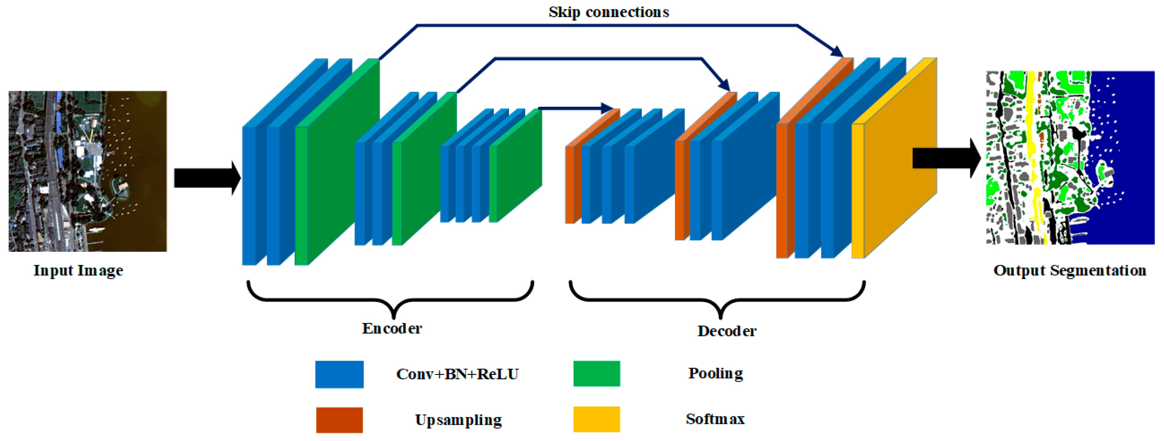
It is noteworthy that an encoder-decoder architecture becomes increasingly popular in semantic segmentation due to its high flexibility and superiority. The illustration of such a CNN architecture is shown in Figure 1. An input image goes through the encoder part first to generate down-sampled feature maps, which consists of several convolution (Conv) layers and max-pooling layers in sequence. To obtain better convergence of deep networks, each Conv layer is followed by Batch Normalization (BN) and Rectified Linear Unit (ReLU) layers. Then, the decoder part is implemented for up-sampling the feature maps to the same size as the original image, where up-sampling layers are followed by several Conv layers to produce dense features with finer resolution. Finally, a softmax layer is added to generate a final segmentation map. The structures of the encoder and decoder parts are symmetrical with skip connections between them, which proves to be effective to produce fine-grained segmentation results.
The mostly used encoder-decoder example is SegNet [64], where unpooling operation is included for better up-sampling. However, skip connections are ignored, leading to poor spatial accuracy. UNet, an extension of SegNet by adding skip connections between the encoder and decoder layers, has better spatial accuracy and achieves great success in semantic segmentation on both medical images [65] and RS images [66]. Recently, Zhou et al. [58] proposed a novel medical image segmentation architecture named UNet++, which can be considered as an extension of UNet. To reduce the semantic gap between the feature maps from the encoder and decoder sub-networks, UNet++ uses a series of nested and dense skip pathways, rather than only connections between encoder and decoder networks. The UNet++ architecture possesses the advantages of capturing fine-grained details, thereby generating better segmentation results than UNet. Therefore, it is promising to exploit the potential of UNet++ for semantic segmentation on RS images.
3. Methodology
In this section, the proposed network architecture is illustrated in detail first. Then, the loss function formulation is discussed. Finally, we present detailed information on the training and prediction.
3.1. Proposed Network Architecture
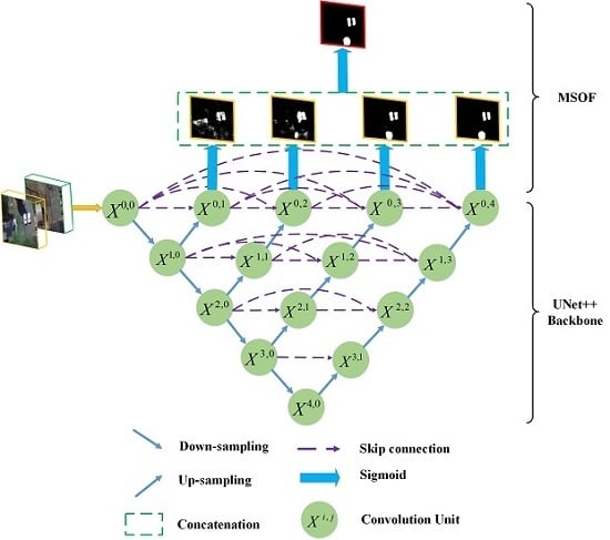
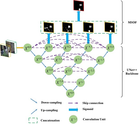
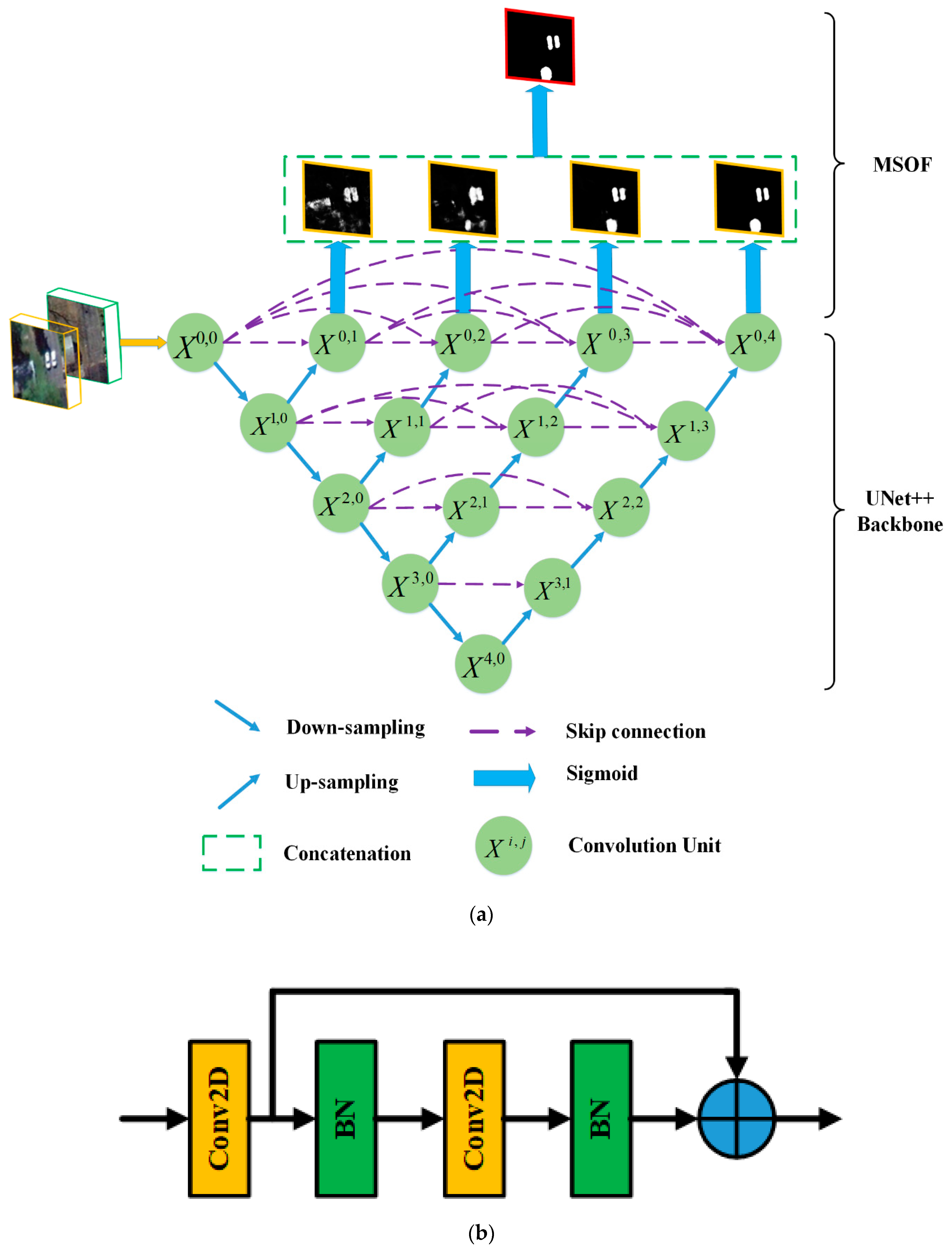
Because CD can be treated as a problem of binary image segmentation, it is natural to introduce advanced semantic segmentation architectures to solve CD tasks. To perform CD on VHR images, we, inspired by UNet++, developed an end-to-end architecture. The flowchart of the proposed method is illustrated in Figure 2. Two periods of images are concatenated as the input of the network, which proves to be effective for learning bi-temporal changes through deep supervised training [53]. Then, the UNet++ model with dense skip connections is adopted as the backbone to learn multiscale and different semantic levels of visual features representations. To further improve the spatial details, DS is implemented by using multiple side-output fusion (MSOF). Finally, a sigmoid layer is followed to generate the final CM.
3.1.1. Backbone of UNet++
UNet++ with nested dense skip pathways has great benefits for extracting multi-scale feature maps from multi-level convolution pathways, which is similar to a UNet architecture, a normal UNet++ architecture consisting of convolution units, down-sampling and up-sampling modules, and skip connections between convolution units, as shown in Figure 2a. The most significant difference between UNet++ and UNet is the re-designed skip pathways, which adopts the same dense connection strategy as DenseNet [67]. Take node as an example, where only one skip connection is applied from node in the UNet architecture, while in UNet++, node receives the skip connections from all previous convolution units at the same level, namely , , and . In such a way, the semantic levels of the encoder feature maps are closer to those in the corresponding decoder part, which facilitates the optimization of the optimizer. Assume represents the output of node , where denotes the ith down-sampling layer along the encoder way, denotes the jth convolution layer along the skip pathway. The accumulation of feature maps by can be expressed as:
where represents a convolution operation followed by an activation function, is an up-sampling layer, and denotes the concatenation operation. In general, nodes at level j of =0 receive only one input from a previous down-sampling layer, while nodes at level j of >0 receive inputs from both the skip pathways and the up-sampling layer. For example, denotes receives the input from node , and then a convolution operation and activation function are applied. denotes nodes , the up-sampling results of node are concatenated first, and then a convolution operation and an activation function are adopted to generate node . It is noteworthy that residual modules are adopted in our convolution unit, which facilitates better convergence abilities for our deep networks. As seen in Figure 2b, a 2-D convolution layer (Conv2D) is implemented first, which is followed by a BN layer. Then, a further Conv2D and BN layer is applied. Finally, the output will be generated by adding the outputs from the second BN layer and the first Conv2D layer. It should be noted that scaled exponential linear units (SeLUs) is adopted as the activation function instead of ReLU, which allows for employing stronger regularization schemes and making learning highly robust [68].
Another major difference is the multi-level full-resolution feature maps-generating strategy. Only a single-level feature map is generated in the UNet architecture through the pathway , as illustrated in Figure 2a. While in UNet++, another three full-resolution feature maps are also obtained, through the pathways }, }, and }, respectively. Thus, the strengths of the four full-resolution feature maps could be combined, which is also beneficial for later DS.
3.1.2. Deep Supervision by Multiple Side-Outputs Fusion
DS is usually implemented by means of supervising side-output layers through auxiliary classifiers [69]. On the one hand, DS improves the convergence of deep networks by overcoming the vanishing gradient problems. On the other hand, more meaningful features ranging from low to high levels could be learned. In [57], DS is implemented by averaging the outputs from all segmentation branches, which fails to work for our CD task. Instead, an MSOF strategy is utilized, which is similar to the one proposed in [70].
As shown in Figure 2a, for the four output nodes , a sigmoid layer is followed to obtain side output results . Then, a new output node could be generated by concatenating the four side output results:
where denotes the concatenation operation. Again, is followed by a sigmoid layer, and the fusion output could thus be generated. Therefore, five outputs are generated in our deep networks, namely , where is the fusion output of . Through the MSOF operation, multi-level features information from all side-output layers are embedded in the final output , which is capable of capturing finer spatial details.
3.2. Loss Function Formulation
In our proposed FCN architecture, five output layers are generated after the classifiers of sigmoid layers. Suppose the corresponding weights are denoted as . Then, the overall loss function could be defined as:
where denotes the loss from the ith side output, which is employed by combining balanced binary cross-entropy and dice coefficient loss:
where denotes the balanced binary cross-entropy loss, is the dice coefficient loss, and refers to the weight that balances the two losses.
3.2.1. Balanced Binary Cross-Entropy Loss
For CD tasks of satellite images, the distributions of changed/unchanged pixels are heavily biased. In particular, some areas are covered by only changed or unchanged pixels, which leads to serious class imbalance problems during deep neural network training. Hence, trade-off parameters have to be introduced for biased sampling. In our end-to-end training manner, the loss function is computed over all pixels in a training image pair and CM , A simple automatically balancing strategy is adopted, and the class-balanced cross-entropy loss function can be defined as:
where and , and represent the numbers of changed and unchanged pixels in the ground truth label images, respectively, and is the sigmoid output at pixel j.
3.2.2. Dice Coefficient Loss
To improve segmentation performance and weaken the effect of class imbalance problems, dice coefficient loss is usually applied in semantic segmentation tasks. In general, the similarity of two contour regions can be defined by dice coefficient. Moreover, the dice coefficient loss could be defined as:
where and denote the predicted probabilities and the ground truth labels of a training image pair, respectively.
3.3. Training and Prediction
The proposed method is implemented by Keras with TensorFlow as the backend, which is powered by a workstation with Intel Xeon CPU W-2123 (3.6 GHz, 8 cores, and 32GB RAM) and a single NVIDIA GTX 1080 Ti GPU. During the training process, Adam optimizer with a learning rate of 1 × 10⁻⁴ is applied. Based on the GPU memory, the batch size is set to 8 for 15 epochs, and the learning rate drops after every 5 epochs. As our proposed architecture is an FCN-based model, it is easy to train the model in an end-to-end manner for an arbitrary size of input images. After training, test images could be fed into the trained model to generate the prediction result. For a image patch with size of , it takes about 0.0447 s to predict the final CD map, which is of high efficiency.
To contribute to the geoscience community, the implementation of our proposed method will be released through GitHub (https://github.com/daifeng2016/End-to-end-CD-for-VHR-satellite-image).
4. Experiments and Results
In this section, several experiments are carried out to verify the effectiveness of our proposed method. First, we present a description of the VHR image dataset, which is provided in [54]. Evaluation metrics are also provided in detail for quantitative analysis of our method. Second, SOTA methods are presented for comparisons. Then, a sensitive analysis of the parameters and the experimental setups is described in detail. Finally, we give a comprehensive analysis of the experimental results.
4.1. Datasets and Evaludation Metrics
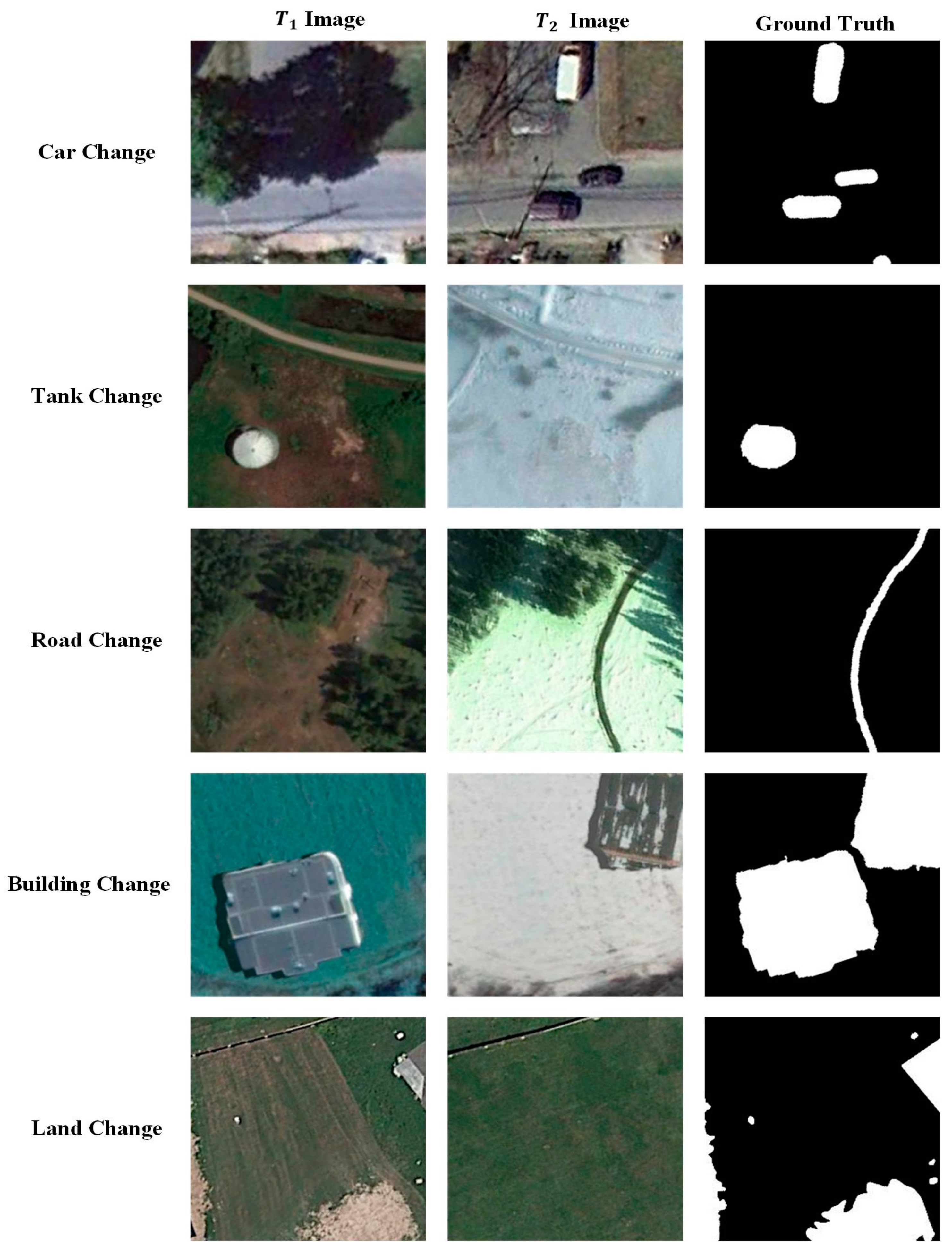
It has to be mentioned that CD tasks have long been hindered for the lack of open datasets, which are crucial for fair and effective comparisons of different algorithms. As a large amount of labeled data are needed for training deep neural networks, it is impossible to use only a small size of co-registered image pairs, which are adopted in most traditional CD tasks. Fortunately, a publicly available dataset of satellite image pairs are presented by Lebedev [54]. The datasets were obtained by Google Earth, covering season-varying RS images of the same region. There are 11 multi-spectral image pairs in the dataset, including 7 pairs of season-varying images with a size of pixels for creating manual reference maps and 4 pairs of images with a size of pixels for adding additional objects manually. It is noteworthy that the dataset consists of multi-source remotely sensed imagery with resolutions varying from 3 cm to 100 cm per pixel, where the season changes between bi-temporal images vary largely. During the generation of reference maps, only the appearance and disappearance of objects were considered as image changes while ignoring changes due to season differences, brightness, and other factors. On the one hand, the dataset is very challenging for CD using traditional methods; on the other hand, different object changes (such as cars, buildings, and tanks) could be well considered, as illustrated in Figure 3. As it is impossible to train CNNs with large images due to the limitation of GPU, image patches have to be generated. We utilize the image patches generated in [54], which consist of 10,000 training sets and 3000 testing and validation sets, created by cropping a size of randomly rotated fragments with at least a part of the target object.
In order to verify the validity of our proposed method, four evaluation metrics are applied based on the comparisons between the prediction CMs and the ground truth maps, namely Precision (P), Recall (R), F1-score (), and Overall Accuracy (OA). In the CD task, a large value of P denotes a small number of false alarms, and a large value of R represents a small number of missed detections. Meanwhile, F1 and OA reveal the overall performance, where their larger values will lead to better performance. These four evaluation metrics are descried as:
where TP, FP, TN, and FN denote the number of true positives, the number of false positives, the number of true negatives, and the number of false negatives, respectively.
4.2. Comparison Methods
To verify the superiority and effectiveness of our proposed CD method, some SOTA IB-DLCD approaches are compared, which are described as follows:
- (1)
- Change detection network (CDNet) [56] was proposed for pixel-wise CD in street view scenes, which consists of contraction blocks and expansion blocks, and the final CM is generated by a soft-max layer.
- (2)
- Fully convolutional-early fusion (FC-EF) [53] was proposed for CD of satellite images. Image pairs are stacked as the input images. Skip connections are utilized to complement the less localized information with spatial details, thereby producing CMs with precise boundaries.
- (3)
- Fully convolutional Siamese-concatenation (FC-Siam-conc) [53] is a Siamese extension of FC-EF model. The encoding layers are separated into two streams of equal structure with shared weights. Then, the skip connections are concatenated in the decoder part.
- (4)
- Fully convolutional Siamese-difference (FC-Siam-diff) [53] is another Siamese extension of FC-EF model. The skip connections from the encoding streams are concatenated by using the absolute value of their difference.
- (5)
- FC-EF with residual blocks (FC-EF-Res) [51] is employed for CD in high-resolution satellite images. It is an extension of FC-EF architecture, where residual blocks with skip connections are used to improve the spatial accuracy of CM.
- (6)
- Fully convolutional network with pyramid pooling (FCN-PP) [52] is applied for landslide inventory mapping. A U-shape architecture is used to construct the FCN. Additionally, pyramid pooling is utilized to capture wider receptive field and overcome the drawbacks of global pooling.
4.3. Parameter Setting
The size of convolution kernel is set to pixels for all convolutional layers, which can maintain spatial information and increase the computation speed effectively. The number of convolutional filters in the encoder part is set to {32, 64, 128, 256, 512}. As two periods of RGB images with a size of pixels are stacked to feed into the network, the input is a tensor with pixels, while the output is a tensor with pixels. For the proposed loss function, the weight of each side output is set to 1.0, while is set to 0.5 for balancing the weight of binary cross-entropy loss and dice coefficient loss. The effect of loss function, data augmentation, and MSOF will be described in the following subsections. In addition, the parameters of the other competitors are set as illustrated in the literature [51,52,53,56].
4.3.1. Effect of Loss Function
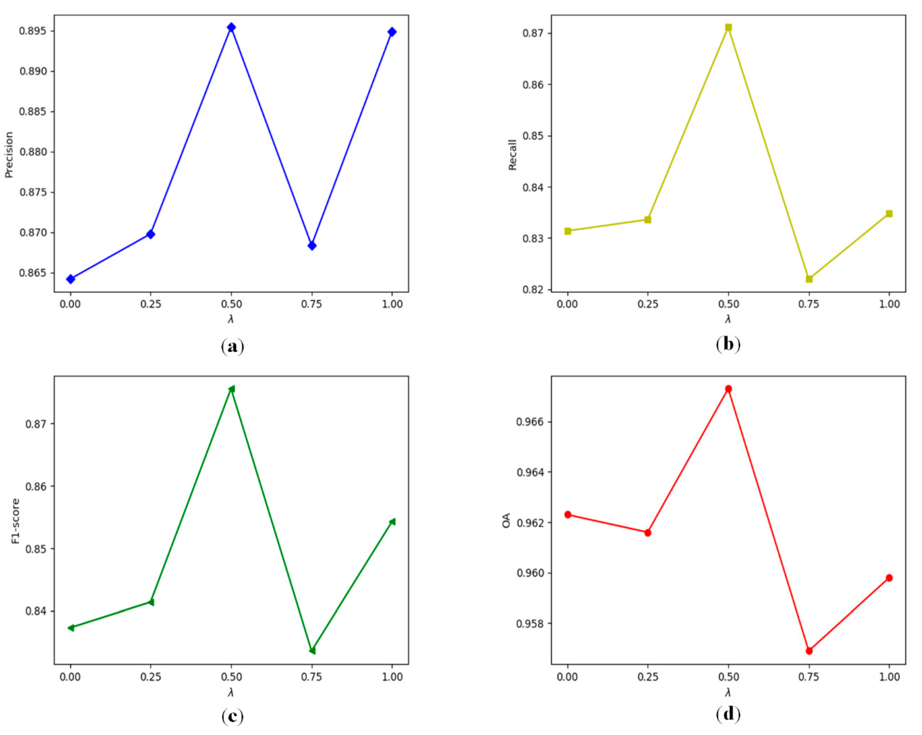
Loss function plays an important role in the final CD results. In particular, the parameter , which balances the weight of binary cross-entropy loss and dice coefficient loss, is of great significance on our proposed loss function. To verify the sensitivity of parameter , we varied from 0 to 1.0, and the corresponding evaluation metrics were calculated, as illustrated in Figure 4. When is set to 0, only binary cross-entropy loss is utilized, where the values of P, R, F1, and OA remain at a low level. Then, the four quantitative evaluation metrics increase with the increase of parameter , which verifies the effectiveness of combining binary cross-entropy loss and dice coefficient loss. Note that P, R, F1, and OA achieve the maximum values when is 0.5, which means that the influence of binary cross-entropy loss and dice coefficient loss are well balanced. However, the values of the four quantitative evaluation metrics show a shock downward trend with the further increase of parameter . Therefore, parameter is set to 0.5 for the sake of better CD performance.
4.3.2. Effect of Data Augmentation
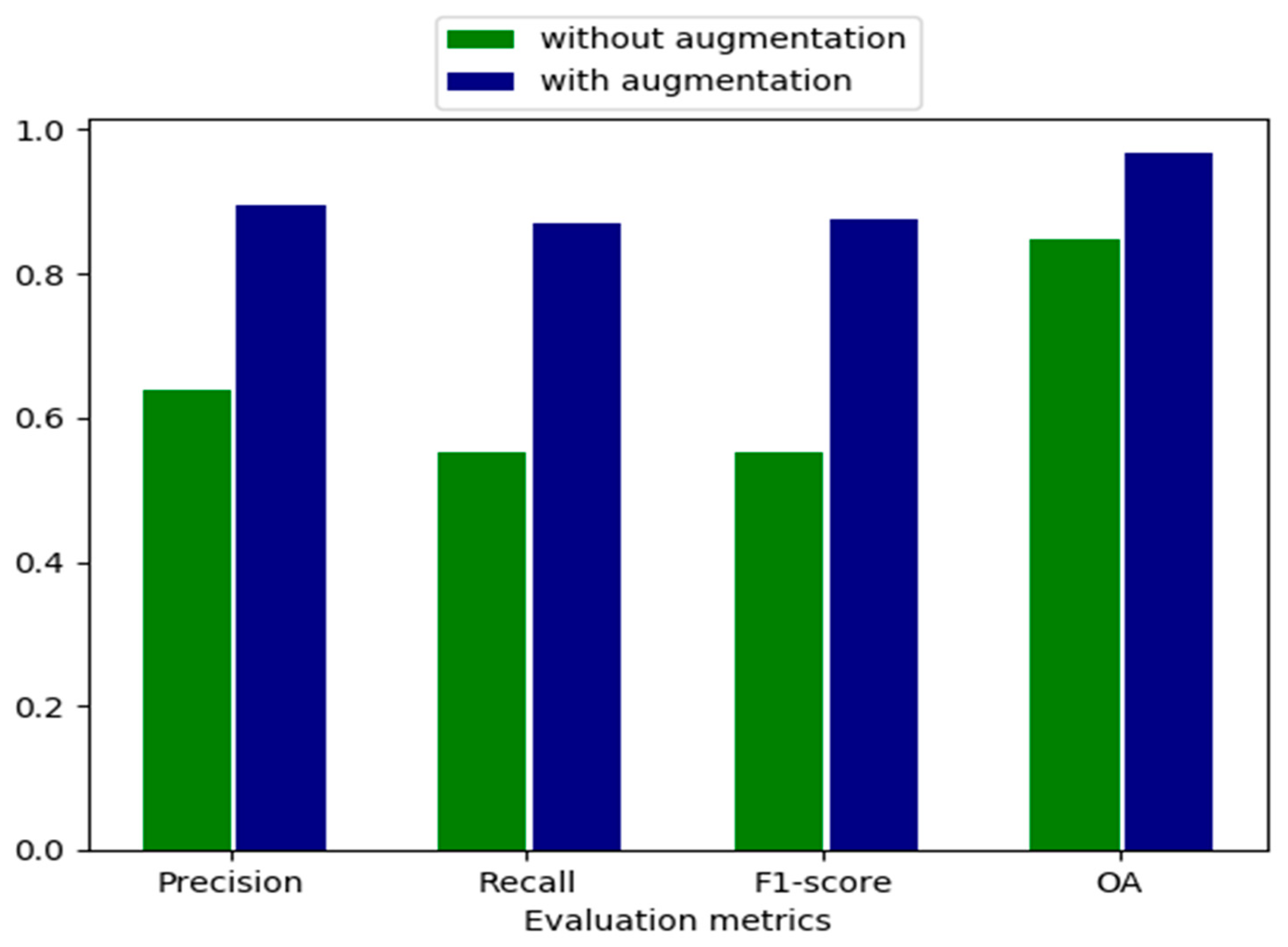
The raw datasets consist of 10,000 training sets and 3000 testing and validation sets, leading to an overfitting problem when training a large network. Because our proposed network contains more than 9 million parameters, it is critical to implement data augmentation to avoid overfitting, as well as improving the generalization ability. To augment the training sets, each image pair is shifted and scaled, rotated by , , and , flipped in horizontal and vertical directions. Figure 5 illustrates the effect of data augmentation by the four quantitative evaluation metrics. We can conclude that the P, R, F1, and OA values can increase by a large margin with data augmentation, which are increased by 40.13%, 57.95%, 58.34%, and 14.01%, respectively. The main reason lies in the fact that 70,000 training sets and 21,000 validation sets are employed after data augmentation, in which case the proposed network parameters can be better learned from more training sets. In addition to this, the overfitting effect can be reduced and the generalization ability of the proposed network can be improved to a large extent. Hence, it is of great significance to implement data augmentation so as to improve the CD accuracy.
4.3.3. Effect of MSOF
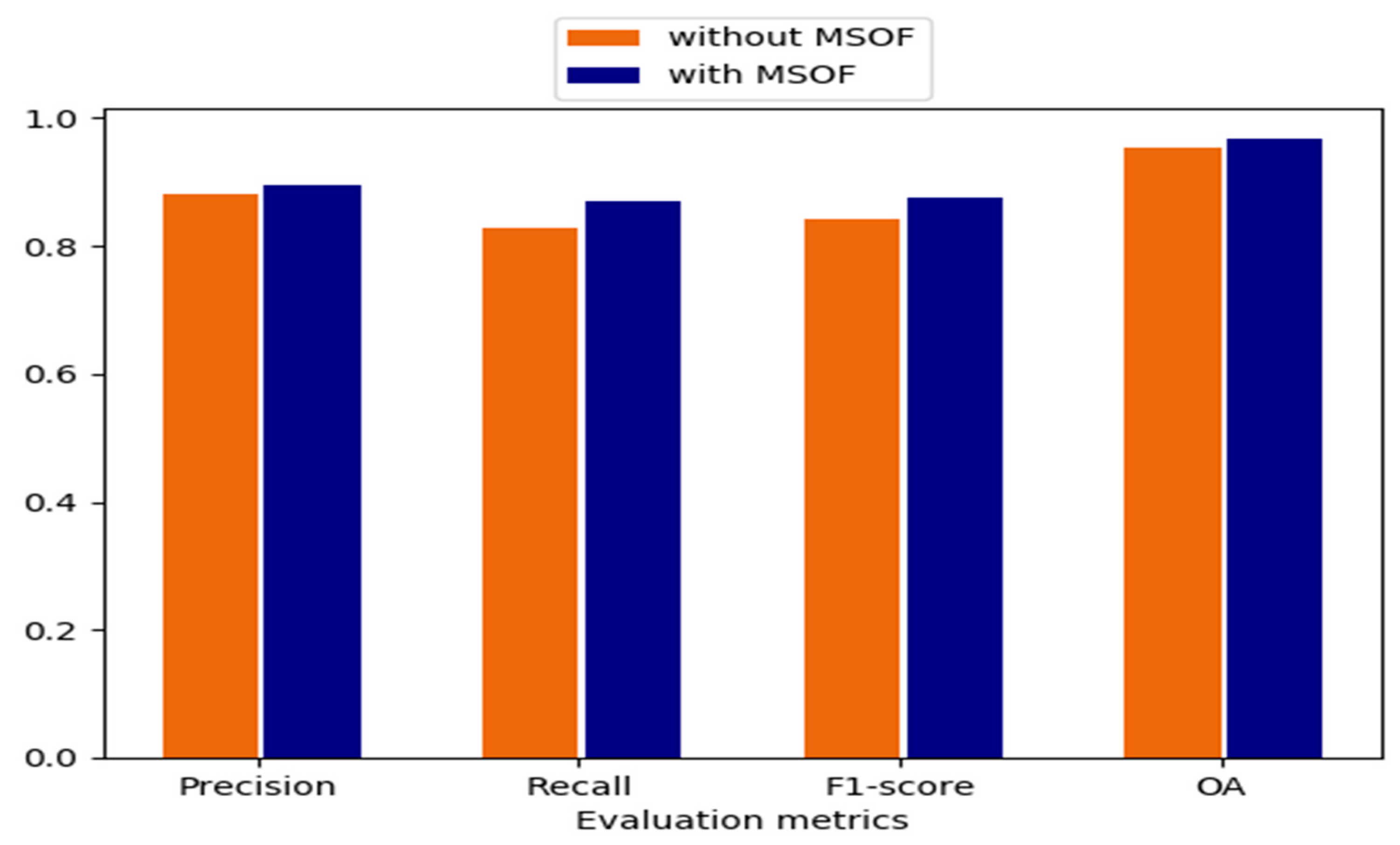
In order to improve the convergence of the proposed deep networks and learn more meaningful features ranging from low to high levels, an MSOF strategy is utilized. Figure 6 presents the influence of MSOF in terms of four quantitative evaluation metrics, namely P, R, F1, and OA. As can be seen, the accuracy of CD can be further improved by the usage of MSOF strategy, where the increase of P, R, F1, and OA are 1.70%, 5.29%, 3.88%, and 1.36%, respectively. This is because feature maps from multiple semantic levels are combined, where more detailed information can be captured. Therefore, MSOF is effective to improve the CD accuracy in our proposed CD method.
4.4. Results Comparisons
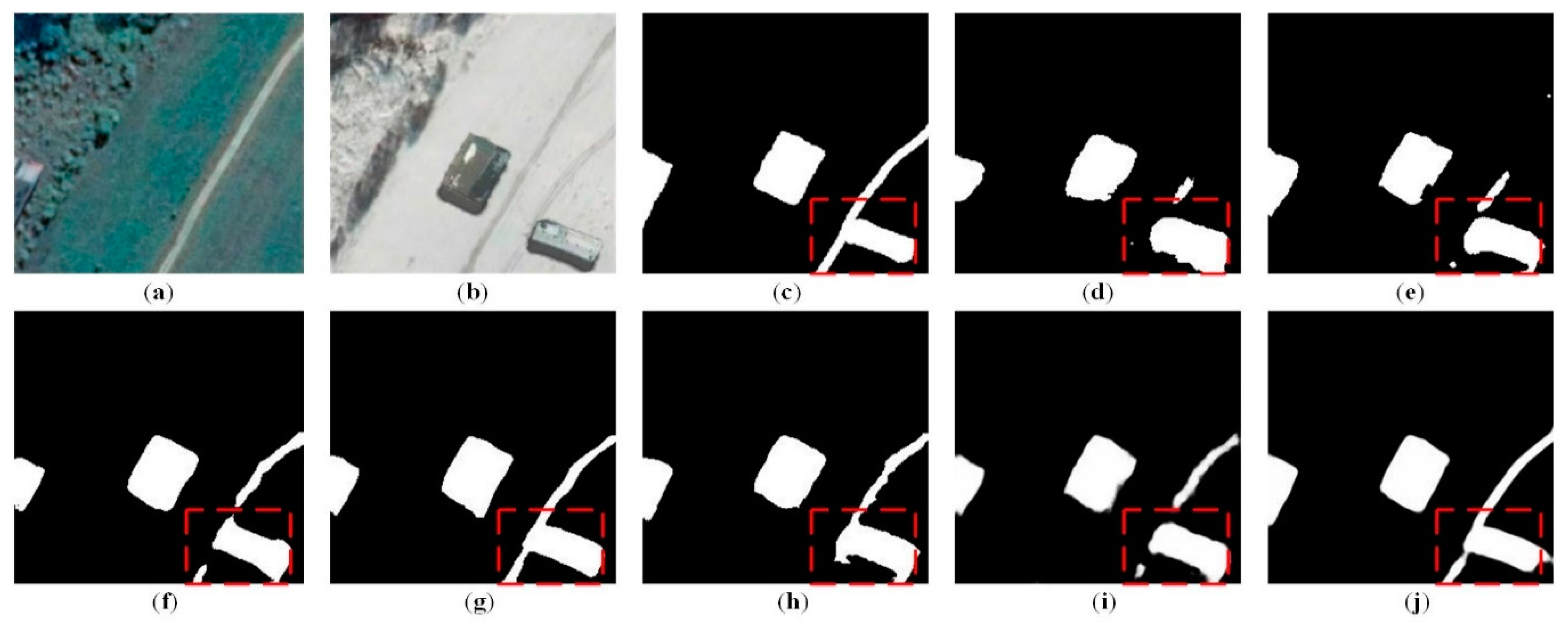
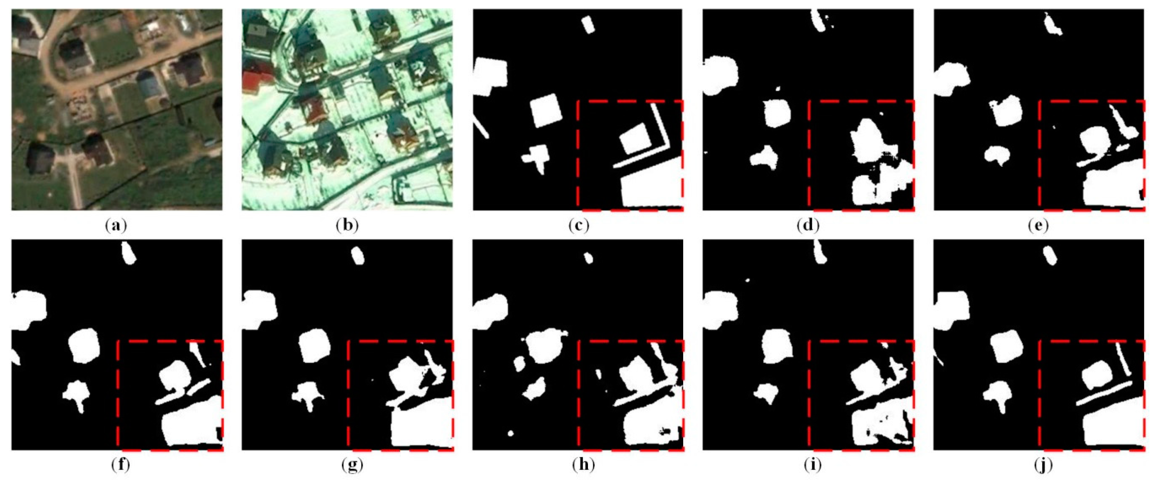
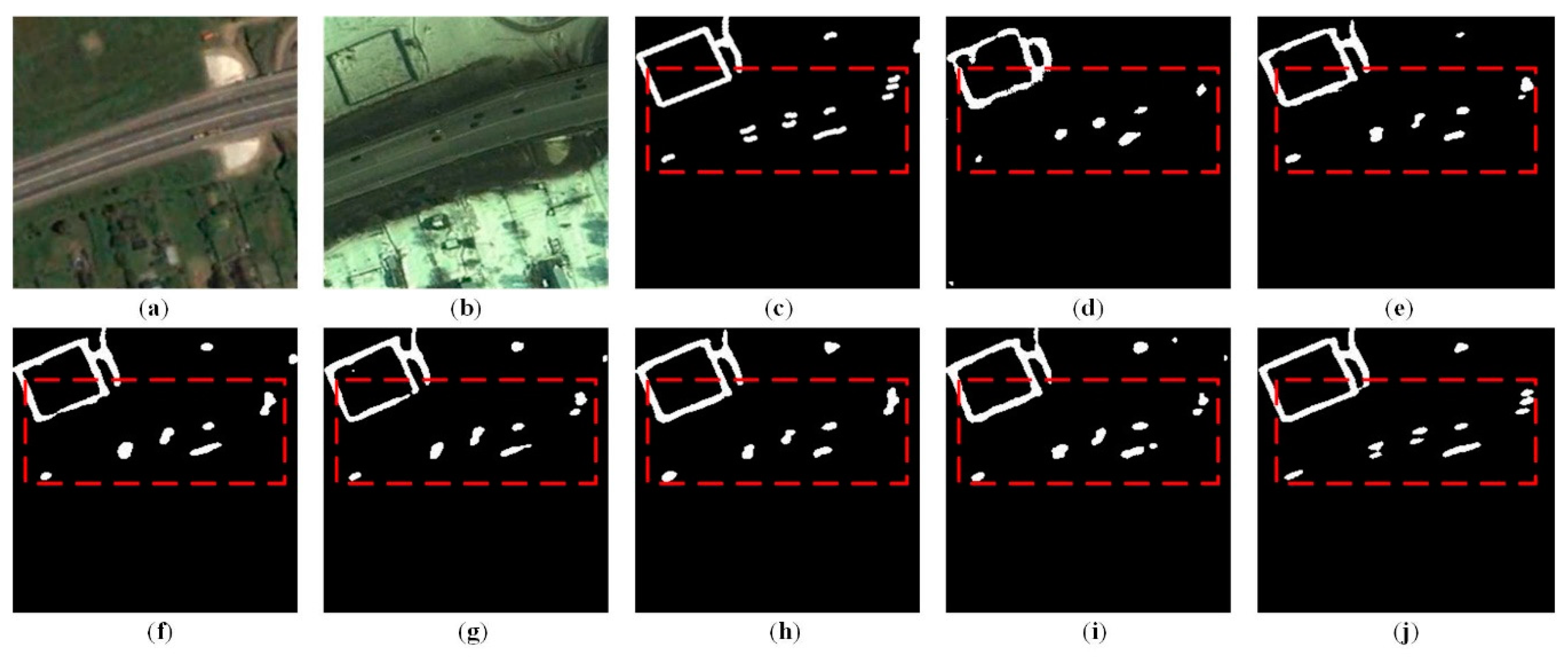
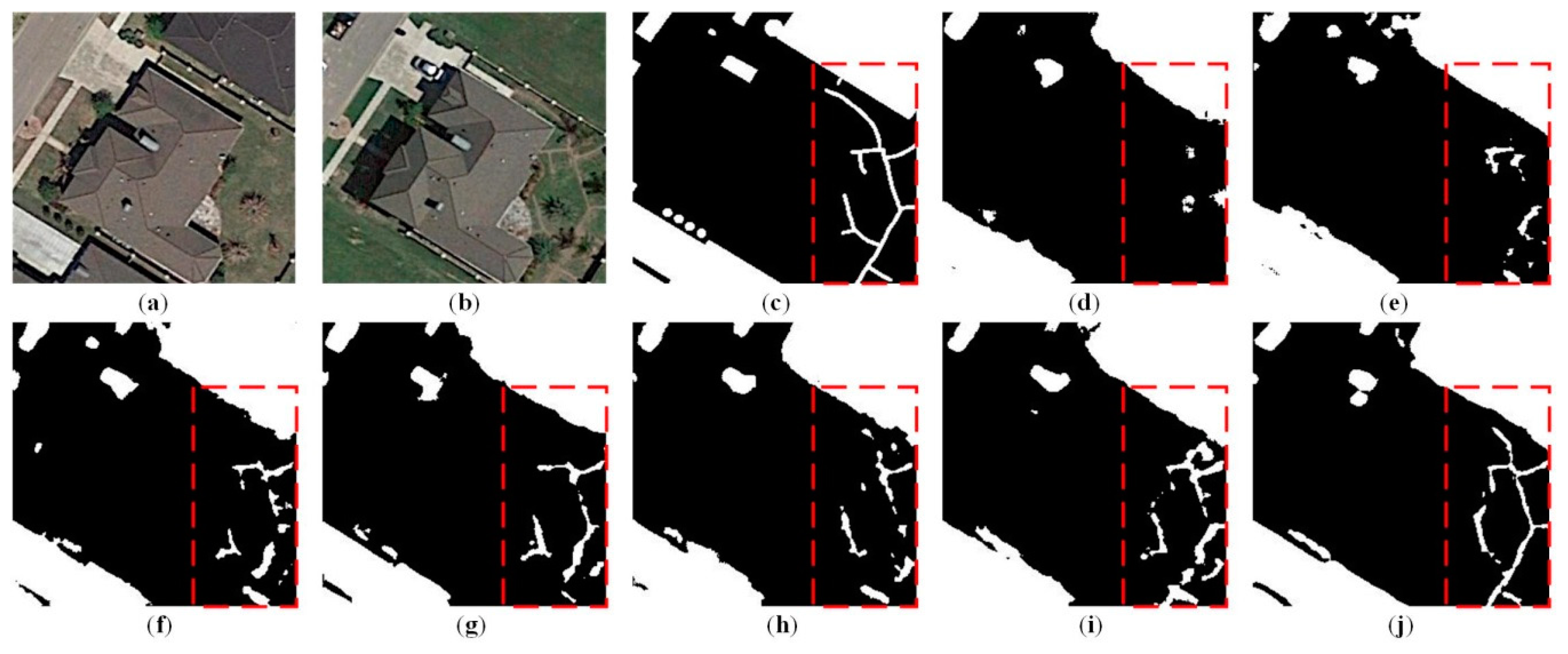
In order to verify the effectiveness and superiority of our proposed CD method, six typical testing areas, which consist of complex changes such as cars, roads, and buildings, are presented for visual comparisons, as illustrated in Figure 7, Figure 8, Figure 9, Figure 10, Figure 11 and Figure 12. It can be observed that the proposed CD method achieves the best CD performance (Figure 7j, Figure 8j, Figure 9j, Figure 10j, Figure 11j and Figure 12j), where the CMs are closely consistent with the reference CMs (Figure 7c, Figure 8c, Figure 9c, Figure 10c, Figure 11c and Figure 12c). In particular, compared with other methods, our approach generates the CMs with more accurate boundaries and less missed detections. As seen in Figure 7 and Figure 8, the boundaries of building changes are clearer and the inner parts are more complete. Note that, compared to the other SOTA methods, our approach achieves the better detection performance for the changes of small objects, e.g., car changes in Figure 9 and Figure 10. In addition, our CD method is also capable of capturing complex and obscure changes, such as long and narrow roads, as seen in Figure 11 and Figure 12. We can see that the road changes can only be partly or coarsely detected by the comparative SOTA methods (Figure 11d–i and Figure 12d–i), while the outlines and locations of the roads are better detected in Figure 11j and Figure 12j.
Meanwhile, for quantitative comparisons, four quantitative evaluation metrics—P, R, F1, and OA—were calculated and are summarized in Table 2. We concluded that the CDNet method obtains the lowest F1 and OA values among all the seven SOTA methods. The reason lies in the fact that the network consists of only contraction and expansion blocks without skip connections between the encoder and decoder parts. Therefore, the detailed information from the low levels was missed in the expansion layers, as can be seen in Figure 7d, Figure 8d, Figure 9d, Figure 10d, Figure 11d and Figure 12d. Based on the UNet backbone, the FC-EF method (Figure 7e, Figure 8e, Figure 9e, Figure 10e, Figure 11e and Figure 12e) achieved better CD results than the CDNet because skip connections were implemented between the encoder blocks and the corresonding decoder blocks, with F1 and OA values increased by 12.05% and 3.88%, respectively. Rather than using traditional convolutional blocks, the FC-EF-Res method adopts residual connections, which greatly facilitates the training of very deep networks, as well as improving the spatial accuracy of the final CM. In order to overcome the drawbacks of global pooling, a pyramid pooling module was integrated into the FCN-PP, where multi-scale features from different convolutional layers were combined to obtain strong feature-representation ability. Therefore, the FC-EF-Res (Figure 7h, Figure 8h, Figure 9h, Figure 10h, Figure 11h and Figure 12h) and FCN-PP (Figure 7i, Figure 8i, Figure 9i, Figure 10i, Figure 11i and Figure 12i) methods achieved better CD results than the FC-EF method, with F1 values increased by 1.95% and 4.36%, respectively, and OA values increased by 0.24% and 1.31%, respectively. Rather than using concatenated image pairs as the input, the Siamese architecture was employed in FC-Siam-conc and FC-Siam-diff, which are two kinds of Siamese extensions of FC-EF model. We concluded that FC-Siam-conc (Figure 7f, Figure 8f, Figure 9f, Figure 10f, Figure 11f and Figure 12f) and FC-Siam-diff (Figure 7g, Figure 8g, Figure 9g, Figure 10g, Figure 11g and Figure 12g) obtained better CD results than FC-EF, with F1 increased by 6.99% and 8.59%, respectively, and OA values increased by 1.69% and 1.72%, respectively. The reasons lie in the fact that the explicit comparisons between image pairs were integrated into Siamese-based skip connections. In particular, difference skip connections could act as the guidance of comparing the difference between image pairs in the architecture, which is the reason why the FC-Siam-diff method achieves even better CD performance than the FC-Siam-conc method.
Note that our CD method (Figure 7j, Figure 8j, Figure 9j, Figure 10j, Figure 11j and Figure 12j) achieved the best performance among all the comparative SOTA methods, with P, R, F1, and OA values reaching 0.8954, 0.8711, 0.8756, and 0.9673, respectively. The reasons lie in the following aspects: (1) UNet++ is utilized as the backbone, where dense skip connections are adopted to learn more powerful multi-scale features from different semantic levels; (2) residual blocks are employed in the convolutional unit of the encoder-decoder architecture, which facilitates the gradient convergence in the proposed deep CNN network, as well as capturing more detailed information; (3) a novel DS method named MSOF is applied in our proposed CD method, which could effectively combine multi-scale feature maps from different semantic levels to generate the final CM; (4) a novel loss function is proposed for our CD task, which combines weighted binary cross-entropy and dice coefficient loss effectively, thereby reducing the class imbalance problem. Compared with CDNet, the proposed CD method achieves the F1 and OA values increased by 27.23% and 6.24%, respectively, which verifies its effectiveness and superiority.
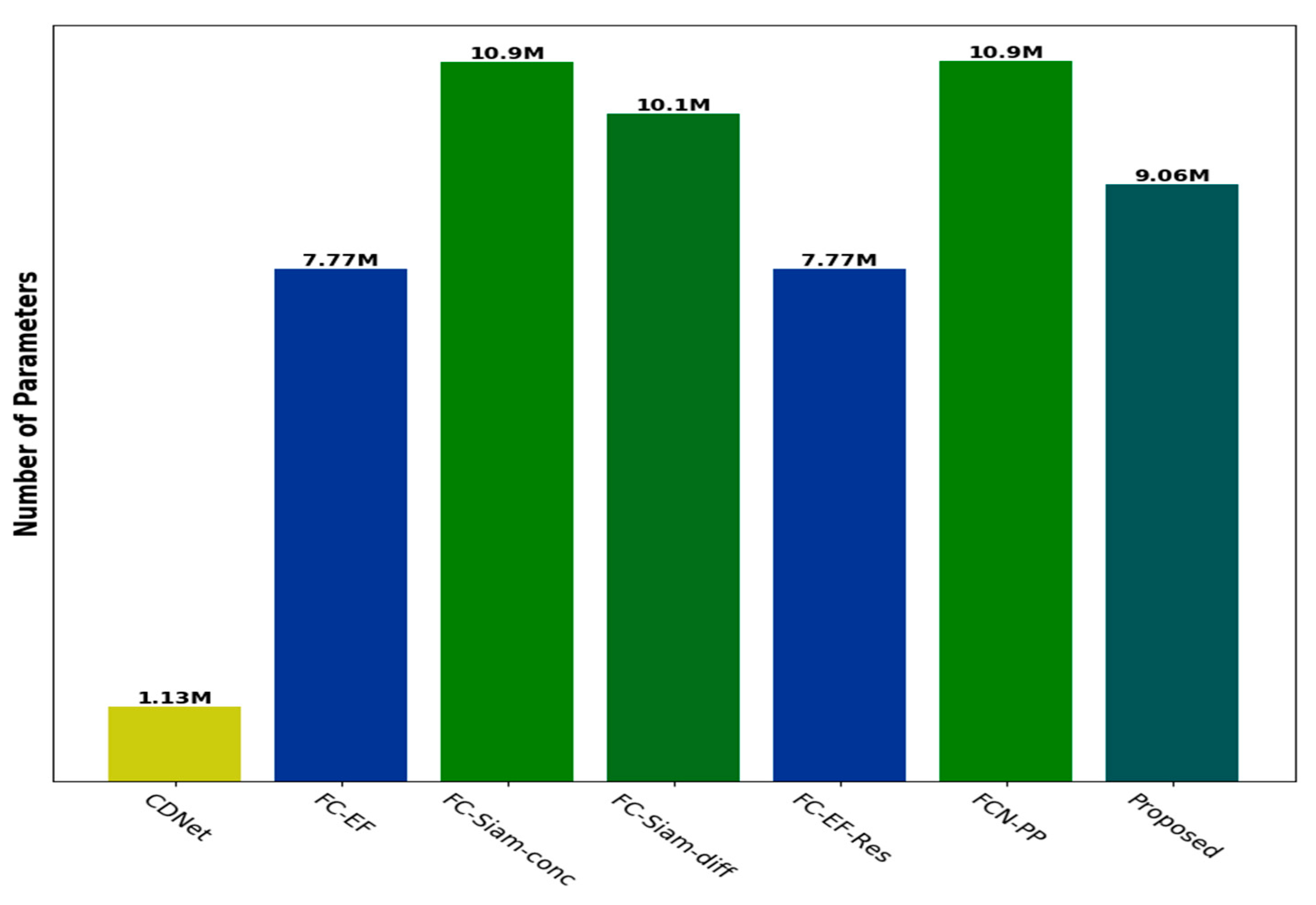
Figure 13 illustrates the number of parameters in different comparative CD approaches. We concluded that CDNet possesses the least network parameters and the worst CD performance (as seen in Table 2). This is because the skip connections are ignored and the change relations between image pairs might not be modeled well using only the simple encoder-decoder architecture. Nevertheless, the skip connections were adopted in the FC-EF model, where the network parameters increase sharply from 1.13 M to 7.77 M, yielding average improvements of F1 and OA values of 0.08 and 0.03, respectively. It should be mentioned that the residual connections might further improve the CD accuracy without any increase of network parameters. That is the reason why the FC-EF-Res method achieves higher F1 and OA values while sharing the same network parameters with the FC-EF. In addition, the FCN-PP method obtains higher F1 and OA values at the cost of increasing network parameters, which are increased by 40.28% compared with the FC-EF method. Due to the additional inner skip connections in the FC-Siam-conc and FC-Siam-diff methods, both the network parameters exceed 10 M, thus increasing the GPU burdens during the training stage to a large extent. It is worth noting that our method achieves the best CD performance with only 9.06 M parameters, which strikes a better balance between CD performance and network parameters.
5. Discussion
Traditional CD methods generally consist of three stages: pre-processing (geometrical rectification, radiometric and atmospheric corrections, image registration, etc.), change information extraction, and accuracy assessment. However, the errors are propagated from the former stages to later stages, which inevitably reduce CD accuracy and reliability. In particular, threshold segmentation is generally utilized in traditional CD methods, which works on the assumptions that the number of changed pixels is proportional to that of the unchanged. However, this is not the real case in some complex scenes. Therefore, it is of great importance to solve CD tasks in an end-to-end manner, where the change relations are learned directly from image pairs. Inspired by the recently developed DL techniques for semantic segmentation, a novel end-to-end CD method was proposed for performing CD tasks on VHR satellite images.
The effectiveness of the proposed CD method was comprehensively examined based on the VHR satellite image datasets. Additionally, the superiority of the proposed CD method was verified through the quantitative and qualitative analysis against several SOTA end-to-end CD methods. Our proposed end-to-end CD model is based on the appearance or disappearance of existing objects while ignoring seasonal changes, and there is no need to implement radiometric corrections, which is a necessary step in traditional CD methods. In addition, the inner change relations between multi-temporal image pairs can be learned from manual interpretation CMs, thereby introducing human domain knowledge effectively. That is especially useful for detecting changes of interest in complex areas, when a large amount of non-interesting changes are unnecessarily detected by using traditional CD methods. It should be noted that, due to the usage of dense skip connections and MSOF strategy, the proposed CD approach is robust to object changes of different scales and sizes, ranging from small cars to large construction structures. This means that our CD method might capture multi-scale object changes, which is critical for detecting objects with sharp changes in sizes and scales on VHR satellite images. Particularly, in difficult areas, our deep neural network model is easily to be fine-tuned by introducing human domain knowledge and adding corresponding samples. In addition, as image pairs are concatenated as the input for our model, it is flexible to include temporal information from more than two periods of images, making it possible to extend the CD task from image pairs to image sequences. Note that our proposed CD model has low computational burden in terms of inference. For example, it takes less than 0.05 s to predict an image with a size of pixels. Therefore, our FCN model provides a promising solution to implement real-time CD once the model is well-trained. As the change relations between multi-temporal images are learned from scratch using available training datasets, the CD results are mainly influenced by: 1) data distribution between the training sets and testing sets; and 2) the accuracy of ground truth maps. When the data distribution is consistent between training sets and testing sets, the trained model will be generalized well to the testing sets and accurate CMs can be produced, otherwise CD results will be greatly influenced. In terms of ground truth maps, only reasonable mapping functions can be learned with high-quality ground truth maps, thereby generating high-accuracy CMs. It is worth noting that although our proposed approach is verified on VHR satellite images, the improved UNet++ itself is independent of raster data forms. This means other forms of 2-D raster data (such as hyperspectral images or multi-channel radar images) can also be applied for CD using our approach; the only difference is the data normalization method before the images are fed into the network.
However, there exist several potential limitations to the proposed method. First, to enlarge the receptive field, the proposed UNet++ architecture utilizes the down-sampling and up-sampling strategy, where the size of feature maps will be half of the inputs after down-sampling while twice the inputs after up-sampling. As four max-pooling layers are applied in the down-sampling part, the size of the feature maps will be one-eighth of the original images size. Therefore, in order to resize the feature maps to the original size after up-sampling operations, the size of the input images should be a multiple of eight (such as 128, 256, and 512). Furthermore, because the proposed FCN architecture contains millions of parameters, a large number of training samples are needed. Due to different sizes and locations of the object changes, it is quite labor-intensive to obtain enough reference CMs with high accuracy. Thus, recently developed DL techniques, such as transfer learning, reinforcement learning, weakly supervised learning, should be exploited for our network to solve the issues of a limited number of training samples.
6. Conclusions
In this paper, an improved UNet++ architecture was proposed for end-to-end CD of VHR satellite images. The dense skip connections within the UNet++ architecture were utilized to learn multi-scale feature maps from different semantic levels. In order to facilitate gradient convergence of the deep FCN network, we adopted a residual block strategy, which was also helpful for capturing more detailed information. In addition to this, the MSOF strategy was adopted to combine multi-scale side-output feature maps and then generate the final CM. To reduce the class imbalance effect, we combined the weighted binary cross-entropy loss and dice coefficient loss effectively. The effectiveness of the proposed method was elaborately examined through the experiments on the VHR satellite image datasets. Compared with other SOTA methods, the proposed approach obtained the best CD performance on both visual comparison and quantitative metrics evaluation. However, the proposed architecture requires a large number of true CMs, which limits the widespread use to a certain extent. In addition, our architecture focuses on only change/no-change information, which is not enough for some practical applications. In the future, we will exploit the potentials of weakly supervised learning and samples generation techniques, as well as investigating the means to build the semantic relations for the changed areas.
Author Contributions
D.P. conceived and designed the experiments, and he also wrote the main manuscript. H.G. and Y.Z. gave comments and suggestions on the manuscript, as well as proofreading the document.
Funding
This work was supported in part by the National Natural Science Foundation of China (under grant numbers: 41801386 and 41671454), in part by the Natural Science Foundation of Jiangsu Province (under grant number: BK20180797), and in part by the Startup Project for Introducing Talent of NUIST (under grant number: 2018r029).
Conflicts of Interest
The authors declare no conflicts of interest.
Abbreviations
The following abbreviations are used in this manuscript
| CD | change detection |
| PBCD | pixel-based change detection |
| OBCD | object-based change detection |
| DI | difference image |
| CM | change map |
| VHR | very-high-resolution |
| DL | deep learning |
| RS | remote sensing |
| FB-DLCD | feature-based deep learning change detection |
| PB-DLCD | patch-based deep learning change detection |
| IB-DLCD | image-based deep learning change detection |
| CNN | convolutional neural network |
| DBN | deep belief network |
| GAN | generative adversarial network |
| cGAN | conditional generative adversarial network |
| IFMN | iterative feature mapping network |
| SDAE | sparse denoising autoencoder |
| RNN | recurrent neural network |
| GDCN | generative discriminatory classified network |
| FCN | fully convolutional network |
| BN | Batch Normalization |
| DS | deep supervision |
| MSOF | multiple side-outputs fusion |
| SOTA | state-of-the-art |
| OA | Overall Accuracy |
| FC-EF | fully convolutional-early fusion |
| FC-Siam-conc | fully convolutional Siamese-concatenation |
| FC-Siam-diff | fully convolutional Siamese-difference |
| FC-EF-Res | fC-EF with residual blocks |
| FCN-PP | fully convolutional network with pyramid pooling |
References
- Singh, A. Review Article Digital change detection techniques using remotely-sensed data. Int. Remote Sens. 2010, 10, 989–1003. [Google Scholar] [CrossRef]
- Tewkesbury, A.P.; Comber, A.J.; Tate, N.J.; Lamb, A.; Fisher, P.F. A critical synthesis of remotely sensed optical image change detection techniques. Remote Sens. Environ. 2015, 160, 1–14. [Google Scholar] [CrossRef] [Green Version]
- Demir, B.; Bovolo, F.; Bruzzone, L. Updating land-cover maps by classification of image time series: A novel change-detection-driven transfer learning approach. IEEE Trans. Geosci. Remote Sens. 2013, 51, 300–312. [Google Scholar] [CrossRef]
- Jin, S.; Yang, L.; Danielson, P.; Homer, C.; Fry, J.; Xian, G. A comprehensive change detection method for updating the National Land Cover Database to circa 2011. Remote Sens. Environ. 2013, 132, 159–175. [Google Scholar] [CrossRef] [Green Version]
- Le Hégarat-Mascle, S.; Ottlé, C.; Guerin, C. Land cover change detection at coarse spatial scales based on iterative estimation and previous state information. Remote Sens. Environ. 2005, 95, 464–479. [Google Scholar] [CrossRef]
- Hussain, M.; Chen, D.; Cheng, A.; Wei, H.; Stanley, D. Change detection from remotely sensed images: From pixel-based to object-based approaches. ISPRS J. Photogramm. Remote Sens. 2013, 80, 91–106. [Google Scholar] [CrossRef]
- Bruzzone, L.; Prieto, D.F. Automatic analysis of the difference image for unsupervised change detection. IEEE Trans. Geosci. Remote Sens. 2000, 38, 1171–1182. [Google Scholar] [CrossRef] [Green Version]
- Celik, T. Unsupervised change detection in satellite images using principal component analysis and k-means clustering. IEEE Geosci. Remote Sens. Lett. 2009, 6, 772–776. [Google Scholar] [CrossRef]
- Deng, J.; Wang, K.; Deng, Y.; Qi, G. PCA-based land-use change detection and analysis using mul-titemporal and multisensor satellite data. Int. J. Remote Sens. 2008, 29, 4823–4838. [Google Scholar] [CrossRef]
- Wu, C.; Du, B.; Cui, X.; Zhang, L. A post-classification change detection method based on iterative slow feature analysis and Bayesian soft fusion. Remote Sens. Environ. 2017, 199, 241–255. [Google Scholar] [CrossRef]
- Huang, C.; Song, K.; Kim, S.; Townshend, J.R.; Davis, P.; Masek, J.G.; Goward, S.N. Use of a dark object concept and support vector machines to automate forest cover change analysis. Remote Sens. Environ. 2008, 112, 970–985. [Google Scholar] [CrossRef]
- Cao, G.; Li, Y.; Liu, Y.; Shang, Y. Automatic change detection in high-resolution remote-sensing images by means of level set evolution and support vector machine classification. Int. J. Remote Sens. 2014, 35, 6255–6270. [Google Scholar] [CrossRef]
- Volpi, M.; Tuia, D.; Bovolo, F.; Kanevski, M.; Bruzzone, L. Supervised change detection in VHR images using contextual information and support vector machines. Int. J. Appl. Earth Obs. Geoinform. 2013, 20, 77–85. [Google Scholar] [CrossRef]
- Benedek, C.; Szir´anyi, T. Change detection in optical aerial images by a multilayer conditional mixed Markov model. IEEE Trans. Geosci. Remote Sens. 2009, 47, 3416–3430. [Google Scholar] [CrossRef]
- Cao, G.; Zhou, L.; Li, Y. A new change detection method in high-resolution remote sensing images based on a conditional random field model. Int. J. Remote Sens. 2016, 37, 1173–1189. [Google Scholar] [CrossRef]
- Lv, P.; Zhong, Y.; Zhao, J.; Zhang, L. Unsupervised change detection based on hybrid conditional random field model for high spatial resolution remote sensing imagery. IEEE Trans. Geosci. Remote Sens. 2018, 56, 4002–4015. [Google Scholar] [CrossRef]
- Jian, P.; Chen, K.; Zhang, C. A hypergraph-based context-sensitive representation technique for VHR remote-sensing image change detection. Int. J. Remote Sens. 2016, 37, 1814–1825. [Google Scholar] [CrossRef]
- Bazi, Y.; Melgani, F.; Al- Sharari, H.D. Unsupervised change detection in multispectral remotely sensed imagery with level set methods. IEEE Trans. Geosci. Remote Sens. 2010, 48, 3178–3187. [Google Scholar] [CrossRef]
- Chen, G.; Hay, G.J.; Carvalho, L.M.; Wulder, M.A. Object-based change detection. Int. J. Remote Sens. 2012, 33, 4434–4457. [Google Scholar] [CrossRef]
- Ma, L.; Li, M.; Blaschke, T.; Ma, X.; Tiede, D.; Cheng, L.; Chen, Z.; Chen, D. Object-based change detection in urban areas: The effects of segmentation strategy, scale, and feature space on unsupervised methods. Remote Sens. 2016, 8, 761. [Google Scholar] [CrossRef]
- Zhang, Y.; Peng, D.; Huang, X. Object-based change detection for VHR images based on multiscale un- certainty analysis. IEEE Geosci. Remote Sens. Lett. 2018, 15, 13–17. [Google Scholar] [CrossRef]
- Gil-Yepes, J.L.; Ruiz, L.A.; Recio, J.A.; Balaguer-Beser, Á.; Hermosilla, T. Description and validation of a new set of object-based temporal geostatistical features for land-use/land-cover change detection. ISPRS J. Photogramm. Remote Sens. 2016, 121, 77–91. [Google Scholar] [CrossRef]
- Qin, Y.; Niu, Z.; Chen, F.; Li, B.; Ban, Y. Object-based land cover change detection for cross-sensor images. Int. J. Remote Sens. 2013, 34, 6723–6737. [Google Scholar] [CrossRef]
- Zhu, X.X.; Tuia, D.; Mou, L.; Xia, G.S.; Zhang, L.; Xu, F.; Fraundorfer, F. Deep learning in remote sensing: A comprehensive review and list of resources. IEEE Geosci. Remote Sens. Mag. 2017, 5, 8–36. [Google Scholar] [CrossRef]
- Zhang, L.; Zhang, L.; Du, B. Deep learning for remote sensing data: A technical tutorial on the state of the art. IEEE Geosci. Remote Sens. Mag. 2016, 4, 22–40. [Google Scholar] [CrossRef]
- Sakurada, K.; Okatani, T. Change Detection from a Street Image Pair using CNN Features and Superpixel Segmentation. In Proceedings of the British Machine Vision Conference BMVC, Swansea, UK, 7–10 September 2015; pp. 61.1–61.12. [Google Scholar]
- Saha, S.; Bovolo, F.; Bruzzone, L. Unsupervised Deep Change Vector Analysis for Multiple-Change De-tection in VHR Images. IEEE Trans. Geosci. Remote Sens. 2019, 57, 3677–3693. [Google Scholar] [CrossRef]
- Hou, B.; Wang, Y.; Liu, Q. Change Detection Based on Deep Features and Low Rank. IEEE Geosci. Remote Sens. Lett. 2017, 14, 2418–2422. [Google Scholar] [CrossRef]
- El Amin, A.M.; Liu, Q.; Wang, Y. Zoom out cnns features for optical remote sensing change detection. In Proceedings of the 2017 2nd International Conference on Image, Vision and Computing (ICIVC), Chengdu, China, 2–4 June 2017; pp. 812–817. [Google Scholar]
- Zhang, H.; Gong, M.; Zhang, P.; Su, L.; Shi, J. Feature-level change detection using deep representation and feature change analysis for multispectral imagery. IEEE Geosci. Remote Sens. Lett. 2016, 13, 1666–1670. [Google Scholar] [CrossRef]
- Zhan, Y.; Fu, K.; Yan, M.; Sun, X.; Wang, H.; Qiu, X. Change detection based on deep siamese convolutional network for optical aerial images. IEEE Geosci. Remote Sens. Lett. 2017, 14, 1845–1849. [Google Scholar] [CrossRef]
- Zhang, M.; Xu, G.; Chen, K.; Yan, M.; Sun, X. Triplet-Based Semantic Relation Learning for Aerial Remote Sensing Image Change Detection. IEEE Geosci. Remote Sens. Lett. 2019, 16, 266–270. [Google Scholar] [CrossRef]
- Niu, X.; Gong, M.; Zhan, T.; Yang, Y. A Conditional Adversarial Network for Change Detection in Heterogeneous Images. IEEE Geosci. Remote Sens. Lett. 2019, 16, 45–49. [Google Scholar] [CrossRef]
- Zhan, T.; Gong, M.; Liu, J.; Zhang, P. Iterative feature mapping network for detecting multiple changes in multi-source remote sensing images. ISPRS J. Photogramm. Remote Sens. 2018, 146, 38–51. [Google Scholar] [CrossRef]
- Lei, Y.; Liu, X.; Shi, J.; Lei, C.; Wang, J. Multiscale Superpixel Segmentation with Deep Features for Change Detection. IEEE Access 2019, 7, 36600–36616. [Google Scholar] [CrossRef]
- Gong, M.; Zhan, T.; Zhang, P.; Miao, Q. Superpixel-based difference representation learning for change detection in multispectral remote sensing images. IEEE Trans. Geosci. Remote Sens. 2017, 55, 2658–2673. [Google Scholar] [CrossRef]
- Gong, M.; Niu, X.; Zhang, P.; Li, Z. Generative adversarial networks for change detection in multi- spectral imagery. IEEE Geosci. Remote Sens. Lett. 2017, 14, 2310–2314. [Google Scholar] [CrossRef]
- Arabi, M.E.A.; Karoui, M.S.; Djerriri, K. Optical Remote Sensing Change Detection Through Deep Siamese Network. In Proceedings of the IGARSS 2018—2018 IEEE International Geoscience and Remote Sensing Symposium, Valencia, Spain, 22–27 July 2018; pp. 5041–5044. [Google Scholar]
- Dong, H.; Ma, W.; Wu, Y.; Gong, M.; Jiao, L. Local Descriptor Learning for Change Detection in Synthetic Aperture Radar Images via Convolutional Neural Networks. IEEE Access 2019, 7, 15389–15403. [Google Scholar] [CrossRef]
- Ma, W.; Xiong, Y.; Wu, Y.; Yang, H.; Zhang, X.; Jiao, L. Change Detection in Remote Sensing Images Based on Image Mapping and a Deep Capsule Network. Remote Sens. 2019, 11, 626. [Google Scholar] [CrossRef]
- Zhang, Z.; Vosselman, G.; Gerke, M.; Tuia, D.; Yang, M.Y. Change Detection between Multimodal Remote Sensing Data Using Siamese CNN. arXiv 2018, arXiv:1807.09562. [Google Scholar]
- Khan, S.H.; He, X.; Porikli, F.; Bennamoun, M. Forest change detection in incomplete satellite images with deep neural networks. IEEE Trans. Geosci. Remote Sens. 2017, 55, 5407–5423. [Google Scholar] [CrossRef]
- Gong, M.; Zhao, J.; Liu, J.; Miao, Q.; Jiao, L. Change detection in synthetic aperture radar images based on deep neural networks. IEEE Trans. Neural Netw. Learn. Syst. 2016, 27, 125–138. [Google Scholar] [CrossRef]
- Daudt, R.C.; Le Saux, B.; Boulch, A.; Gousseau, Y. Urban change detection for multispectral earth observation using convolutional neural networks. arXiv 2018, arXiv:1810.08468. [Google Scholar]
- Wang, Q.; Yuan, Z.; Du, Q.; Li, X. GETNET: A General End-to-End 2-D CNN Framework for Hyper- spectral Image Change Detection. IEEE Trans. Geosci. Remote Sens. 2018, 57, 3–13. [Google Scholar] [CrossRef]
- Wiratama, W.; Lee, J.; Park, S.E.; Sim, D. Dual-Dense Convolution Network for Change Detection of High-Resolution Panchromatic Imagery. Appl. Sci. 2018, 8, 1785. [Google Scholar] [CrossRef]
- Zhang, W.; Lu, X. The Spectral-Spatial Joint Learning for Change Detection in Multispectral Imagery. Remote Sens. 2019, 11, 240. [Google Scholar] [CrossRef]
- Lyu, H.; Lu, H.; Mou, L. Learning a transferable change rule from a recurrent neural network for land cover change detection. Remote Sens. 2016, 8, 506. [Google Scholar] [CrossRef]
- Mou, L.; Bruzzone, L.; Zhu, X.X. Learning spectral-spatial-temporal features via a recurrent convolutional neural network for change detection in multispectral imagery. IEEE Trans. Geosci. Remote Sens. 2019, 57, 924–935. [Google Scholar] [CrossRef]
- Gong, M.; Yang, Y.; Zhan, T.; Niu, X.; Li, S. A Generative Discriminatory Classified Net- work for Change Detection in Multispectral Imagery. IEEE J. Sel. Top. Appl. Earth Obs. Remote Sens. 2019, 12, 321–333. [Google Scholar] [CrossRef]
- Daudt, R.C.; Le Saux, B.; Boulch, A.; Gousseau, Y. High Resolution Semantic Change Detection. arXiv 2018, arXiv:1810.08452v1. [Google Scholar]
- Lei, T.; Zhang, Y.; Lv, Z.; Li, S.; Liu, S.; Nandi, A.K. Landslide Inventory Mapping from Bi-temporal Images Using Deep Convolutional Neural Networks. IEEE Geosci. Remote Sens. Lett. 2019, 16, 982–986. [Google Scholar]
- Daudt, R.C.; Le Saux, B.; Boulch, A. Fully convolutional siamese networks for change detection. In Proceedings of the 2018 25th IEEE International Conference on Image Processing (ICIP), Athens, Greece, 7–10 October 2018; pp. 4063–4067. [Google Scholar]
- Lebedev, M.; Vizilter, Y.V.; Vygolov, O.; Knyaz, V.; Rubis, A.Y. Change detection in remote sensing images using conditional adversarial networks. Int. Arch. Photogramm. Remote Sens. Spat. Inf. Sci. 2018, 42, 565–571. [Google Scholar] [CrossRef]
- Guo, E.; Fu, X.; Zhu, J.; Deng, M.; Liu, Y.; Zhu, Q.; Li, H. Learning to Measure Change: Fully Convolutional Siamese Metric Networks for Scene Change Detection. arXiv 2018, arXiv:1810.09111. [Google Scholar]
- Alcantarilla, P.F.; Stent, S.; Ros, G.; Arroyo, R.; Gherardi, R. Streetview change detection with deconvolutional networks. Auton. Robots 2018, 42, 1301–1322. [Google Scholar] [CrossRef]
- Li, X.; Yuan, Z.; Wang, Q. Unsupervised Deep Noise Modeling for Hyperspectral Image Change Detection. Remote Sens. 2019, 11, 258. [Google Scholar] [CrossRef]
- Zhou, Z.; Siddiquee, M.M.R.; Tajbakhsh, N.; Liang, J. Unet++: A nested u-net architecture for medical image segmentation. In Deep Learning in Medical Image Analysis and Multimodal Learning for Clinical Decision Support; Springer: Cham, Switzerland, 2018; pp. 3–11. [Google Scholar]
- L¨angkvist, M.; Kiselev, A.; Alirezaie, M.; Loutfi, A. Classification and segmentation of satellite orthoimagery using convolutional neural networks. Remote Sens. 2016, 8, 329. [Google Scholar] [CrossRef]
- Long, J.; Shelhamer, E.; Darrell, T. Fully convolutional networks for semantic segmentation. In Proceedings of the IEEE conference on computer vision and pattern recognition, Boston, MA, USA, 7–12 June 2015; pp. 3431–3440. [Google Scholar]
- Yu, F.; Koltun, V. Multi-scale context aggregation by dilated convolutions. arXiv 2015, arXiv:1511.07122. [Google Scholar]
- He, K.; Zhang, X.; Ren, S.; Sun, J. Deep residual learning for image recognition. In Proceedings of the IEEE conference on computer vision and pattern recognition, Las Vegas, NV, USA, 27–30 June 2016; pp. 770–778. [Google Scholar]
- He, K.; Zhang, X.; Ren, S.; Sun, J. Spatial pyramid pooling in deep convolutional networks for visual recognition. IEEE Trans. Pattern Anal. Mach. Intell. 2015, 37, 1904–1916. [Google Scholar] [CrossRef]
- Badrinarayanan, V.; Handa, A.; Cipolla, R. Segnet: A deep convolutional encoder-decoder architecture for robust semantic pixel-wise labelling. arXiv 2015, arXiv:1505.07293. [Google Scholar]
- Ronneberger, O.; Fischer, P.; Brox, T. U-net: Convolutional networks for biomedical image segmentation. In Proceedings of the International Conference on Medical Image Computing and Computer-Assisted Intervention, Munich, Germany, 5–9 October 2015; pp. 234–241. [Google Scholar]
- Kim, J.H.; Lee, H.; Hong, S.J.; Kim, S.; Park, J.; Hwang, J.Y.; Choi, J.P. Objects Segmentation from High-Resolution Aerial Images Using U-Net With Pyramid Pooling Layers. IEEE Geosci. Remote Sens. Lett. 2019, 16, 115–119. [Google Scholar] [CrossRef]
- Huang, G.; Liu, Z.; Van Der Maaten, L.; Weinberger, K.Q. Densely connected convolutional networks. In Proceedings of the IEEE Conference on Computer Vision and Pattern Recognition, Honolulu, HI, USA, 21–26 July 2017; pp. 4700–4708. [Google Scholar]
- Klambauer, G.; Unterthiner, T.; Mayr, A.; Hochreiter, S. Selfnormalizing neural networks. Adv. Neural Inf. Process. Syst. 2017, 30, 971–980. [Google Scholar]
- Lee, C.Y.; Xie, S.; Gallagher, P.; Zhang, Z.; Tu, Z. Deeply-supervised nets. arXiv 2015, arXiv:1409.5185. [Google Scholar]
- Xie, S.; Tu, Z. Holistically-nested edge detection. In Proceedings of the IEEE International Conference on Computer Vision, Santiago, Chile, 7–13 December 2015; pp. 1395–1403. [Google Scholar]
Figure 1.
An illustration of encoder-decoder-based FCN architecture for semantic segmentation.

Figure 2.
Flowchart of the proposed method: (a) illustration of the main flowchart; (b) illustration of the convolution unit.
Figure 2.
Flowchart of the proposed method: (a) illustration of the main flowchart; (b) illustration of the convolution unit.

Figure 3.
An illustration of different object changes.

Figure 4.
The effects of parameter on the accuracy of our CD method: (a) the effect of parameter on Precision; (b) the effect of parameter on Recall; (c) the effect of parameter on F1-score; (d) the effect of parameter on OA.
Figure 4.
The effects of parameter on the accuracy of our CD method: (a) the effect of parameter on Precision; (b) the effect of parameter on Recall; (c) the effect of parameter on F1-score; (d) the effect of parameter on OA.

Figure 5.
The effect of data augmentation on the accuracy of our proposed CD method in terms of Precision, Recall, F1-score, and OA.
Figure 5.
The effect of data augmentation on the accuracy of our proposed CD method in terms of Precision, Recall, F1-score, and OA.

Figure 6.
The effect of multiple side-outputs fusion (MSOF) strategy on the accuracy of our proposed CD method in terms of Precision, Recall, F1-score, and OA.
Figure 6.
The effect of multiple side-outputs fusion (MSOF) strategy on the accuracy of our proposed CD method in terms of Precision, Recall, F1-score, and OA.

Figure 7.
Visual comparisons of change detection results using different approaches for area 1: (a) image , (b) image , (c) reference change map, (d) CDNet, (e) FC-EF, (f) FC-Siam-conc, (g) FC-Siam-diff, (h) FC-EF-Res, (i) FCN-PP, and (j) proposed method. The changed parts are marked in white while the unchanged parts are in black.

Figure 8.
Visual comparisons of change detection results using different approaches for area 2: (a) image , (b) image , (c) reference change map, (d) CDNet, (e) FC-EF, (f) FC-Siam-conc, (g) FC-Siam-diff, (h) FC-EF-Res, (i) FCN-PP, and (j) proposed method. The changed parts are marked in white while the unchanged parts are in black.

Figure 9.
Visual comparisons of change detection results using different approaches for area 3: (a) image , (b) image , (c) reference change map, (d) CDNet, (e) FC-EF, (f) FC-Siam-conc, (g) FC-Siam-diff, (h) FC-EF-Res, (i) FCN-PP, and (j) proposed method. The changed parts are marked in white while the unchanged parts are in black.

Figure 10.
Visual comparisons of change detection results using different approaches for area 4: (a) image , (b) image , (c) reference change map, (d) CDNet, (e) FC-EF, (f) FC-Siam-conc, (g) FC-Siam-diff, (h) FC-EF-Res, (i) FCN-PP, and (j) proposed method. The changed parts are marked in white while the unchanged parts are in black.

Figure 11.
Visual comparisons of change detection results using different approaches for area 5: (a) image , (b) image , (c) reference change map, (d) CDNet, (e) FC-EF, (f) FC-Siam-conc, (g) FC-Siam-diff, (h) FC-EF-Res, (i) FCN-PP, and (j) proposed method. The changed parts are marked in white while the unchanged part are in black.

Figure 12.
Visual comparison of change detection results using different approaches for area 6: (a) image , (b) image , (c) reference change map, (d) CDNet, (e) FC-EF, (f) FC-Siam-conc, (g) FC-Siam-diff, (h) FC-EF-Res, (i) FCN-PP, and (j) proposed method. The changed parts are marked in white while the unchanged are in black.

Figure 13.
A comparison of network parameter size for different methods.


Table 1.
Summary of contemporary CD methods.
| Methods | Category | Example Studies |
|---|---|---|
| Traditional CD methods | PBCD | Bruzzone et al. [7], Celik [8], Deng et al. [9], Wu et al. [10], Huang et al. [11], Benedek et al. [14], and Bazi et al. [18] |
| OBCD | Ma et al. [20], Zhang et al. [21], Gil-Yepes et al. [22], Qin et al. [23] | |
| Deep learning CD methods | FB-DLCD | Sakurada et al. [26], Saha et al. [27], Hou et al. [28], El Amin et al. [29], Zhan et al. [31], Zhang et al. [32], Niu et al. [33], and Zhan et al. [34] |
| PB-DLCD | Gong et al. [36], Arabi et al. [38], Ma et al. [40], Zhang et al. [41], Khan et al. [42], Daudt et al. [44], Wang et al. [45], Wiratama et al. [46], Zhang et al. [47], Mou et al. [49], and Gong et al. [50] | |
| IB-DLCD | Lei et al. [52], Daudy et al. [53], Lebedev et al. [54], and Guo et al. [55] |
Table 2.
Quantitative evaluation results of different approaches, where the best values are in bold.
Table 2.
Quantitative evaluation results of different approaches, where the best values are in bold.
| Methods | Precision | Recall | F1-Score | OA |
|---|---|---|---|---|
| CDNet | 0.7395 | 0.6797 | 0.6882 | 0.9105 |
| FC-EF | 0.8156 | 0.7613 | 0.7711 | 0.9413 |
| FC-Siam-conc | 0.8441 | 0.8250 | 0.8250 | 0.9572 |
| FC-Siam-diff | 0.8578 | 0.8364 | 0.8373 | 0.9575 |
| FC-EF-Res | 0.8093 | 0.7881 | 0.7861 | 0.9436 |
| FCN-PP | 0.8264 | 0.8060 | 0.8047 | 0.9536 |
| Proposed method | 0.8954 | 0.8711 | 0.8756 | 0.9673 |
© 2019 by the authors. Licensee MDPI, Basel, Switzerland. This article is an open access article distributed under the terms and conditions of the Creative Commons Attribution (CC BY) license (http://creativecommons.org/licenses/by/4.0/).
Share and Cite
MDPI and ACS Style
Peng, D.; Zhang, Y.; Guan, H. End-to-End Change Detection for High Resolution Satellite Images Using Improved UNet++. Remote Sens. 2019, 11, 1382. https://0-doi-org.brum.beds.ac.uk/10.3390/rs11111382
AMA Style
Peng D, Zhang Y, Guan H. End-to-End Change Detection for High Resolution Satellite Images Using Improved UNet++. Remote Sensing. 2019; 11(11):1382. https://0-doi-org.brum.beds.ac.uk/10.3390/rs11111382
Chicago/Turabian StylePeng, Daifeng, Yongjun Zhang, and Haiyan Guan. 2019. "End-to-End Change Detection for High Resolution Satellite Images Using Improved UNet++" Remote Sensing 11, no. 11: 1382. https://0-doi-org.brum.beds.ac.uk/10.3390/rs11111382
Note that from the first issue of 2016, this journal uses article numbers instead of page numbers. See further details here.