Complementarity of X-, C-, and L-band SAR Backscatter Observations to Retrieve Forest Stem Volume in Boreal Forest


Abstract
:
1. Introduction
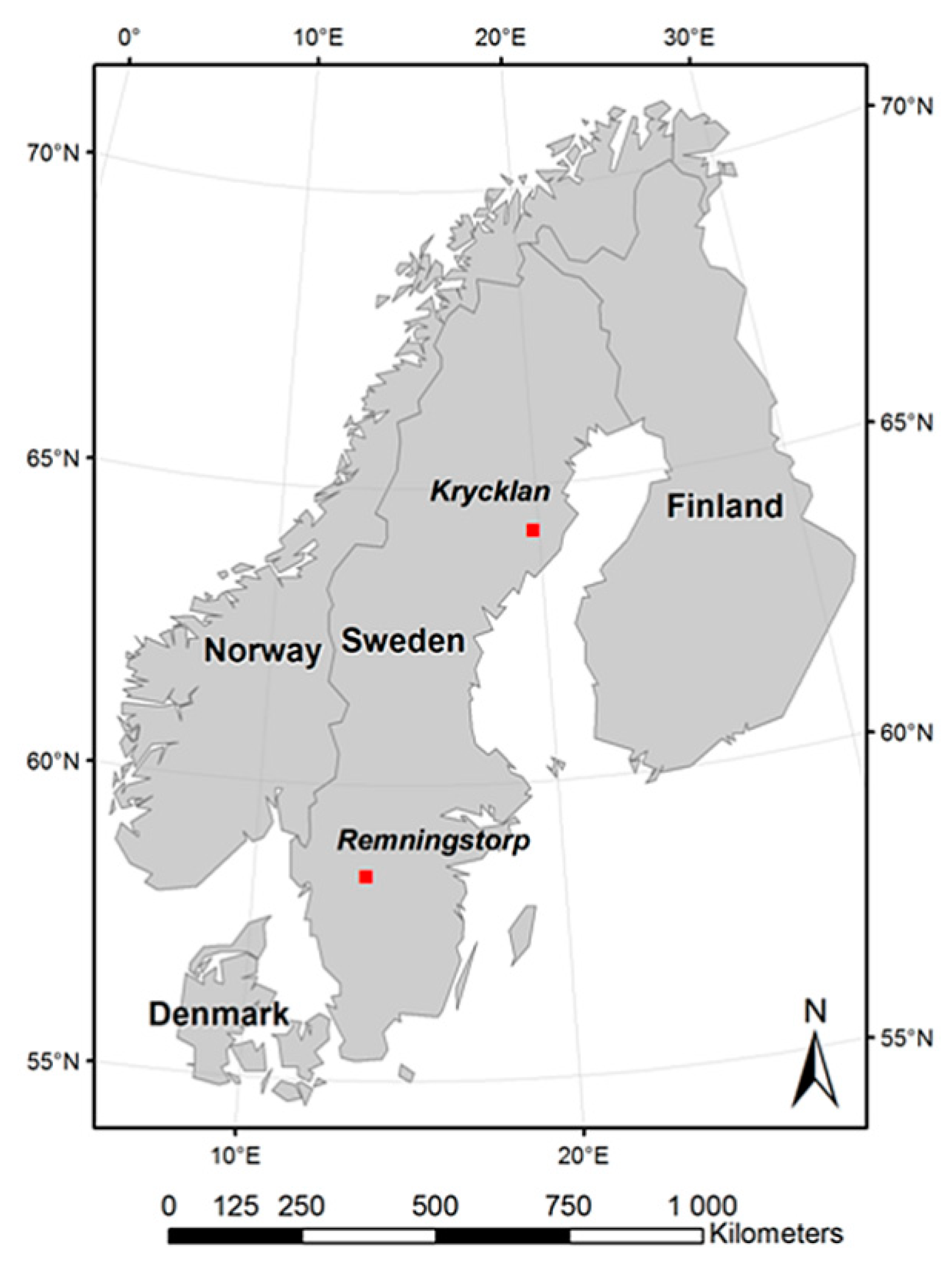
2. Test Sites
3. SAR Datasets
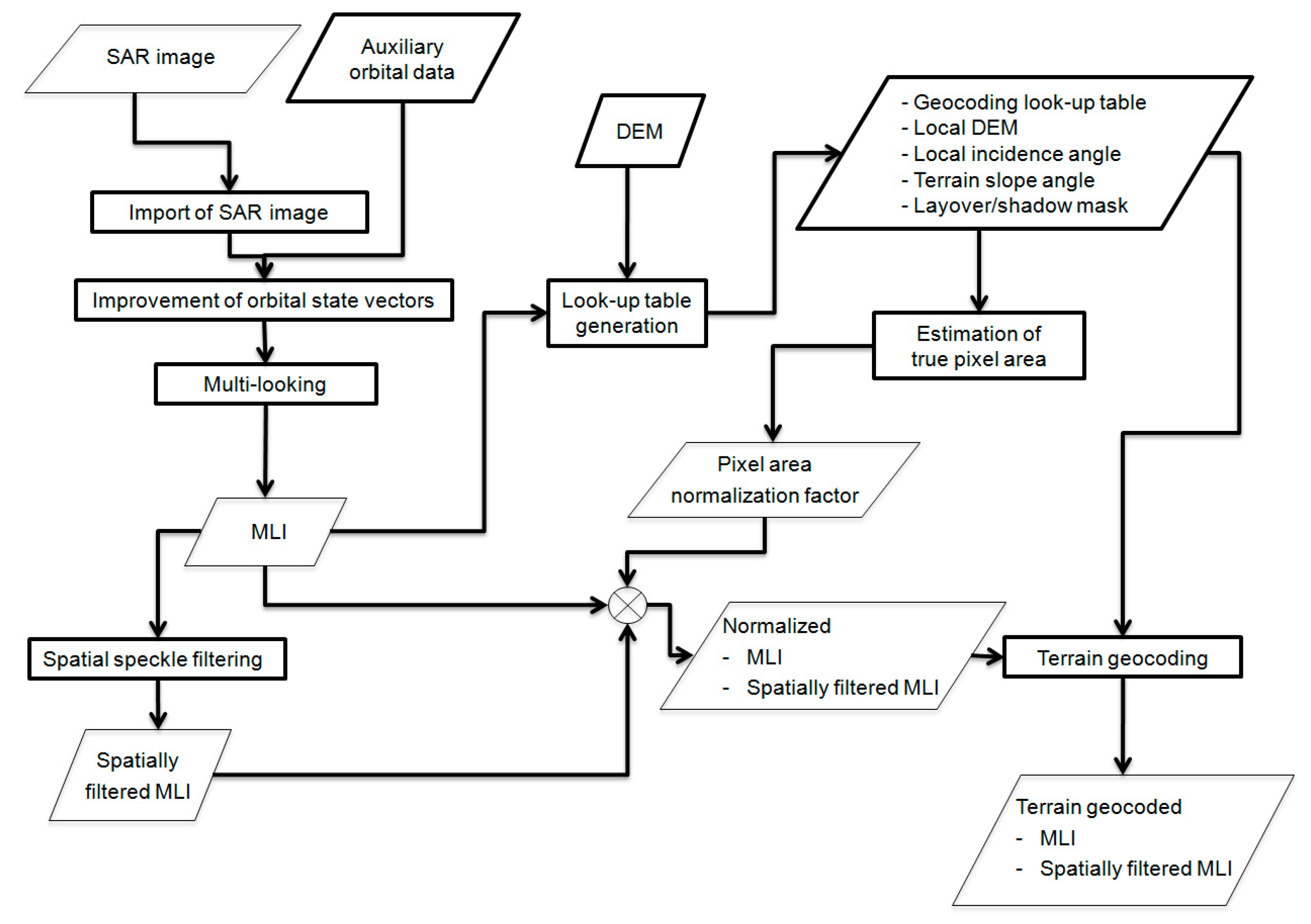
SAR Data Processing
4. Methods
5. Results
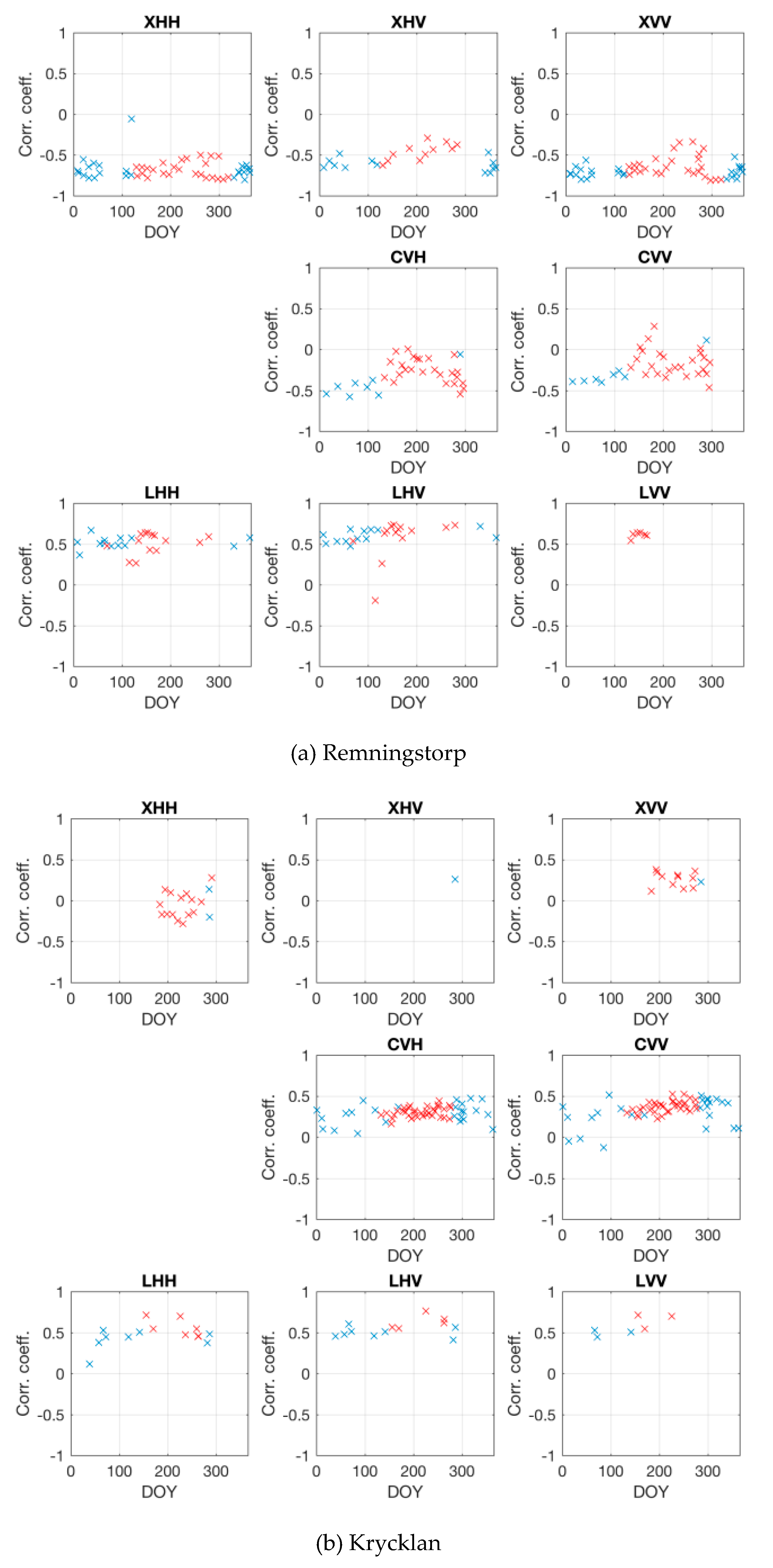
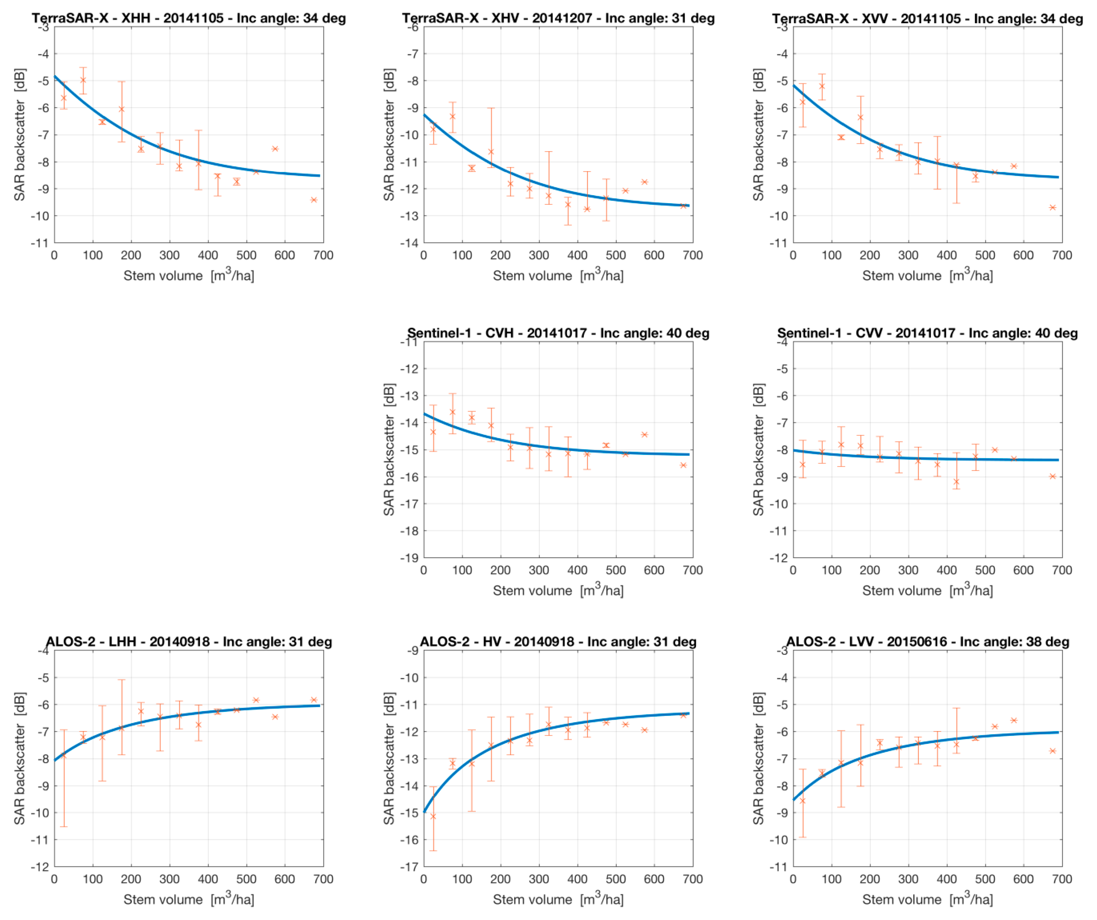
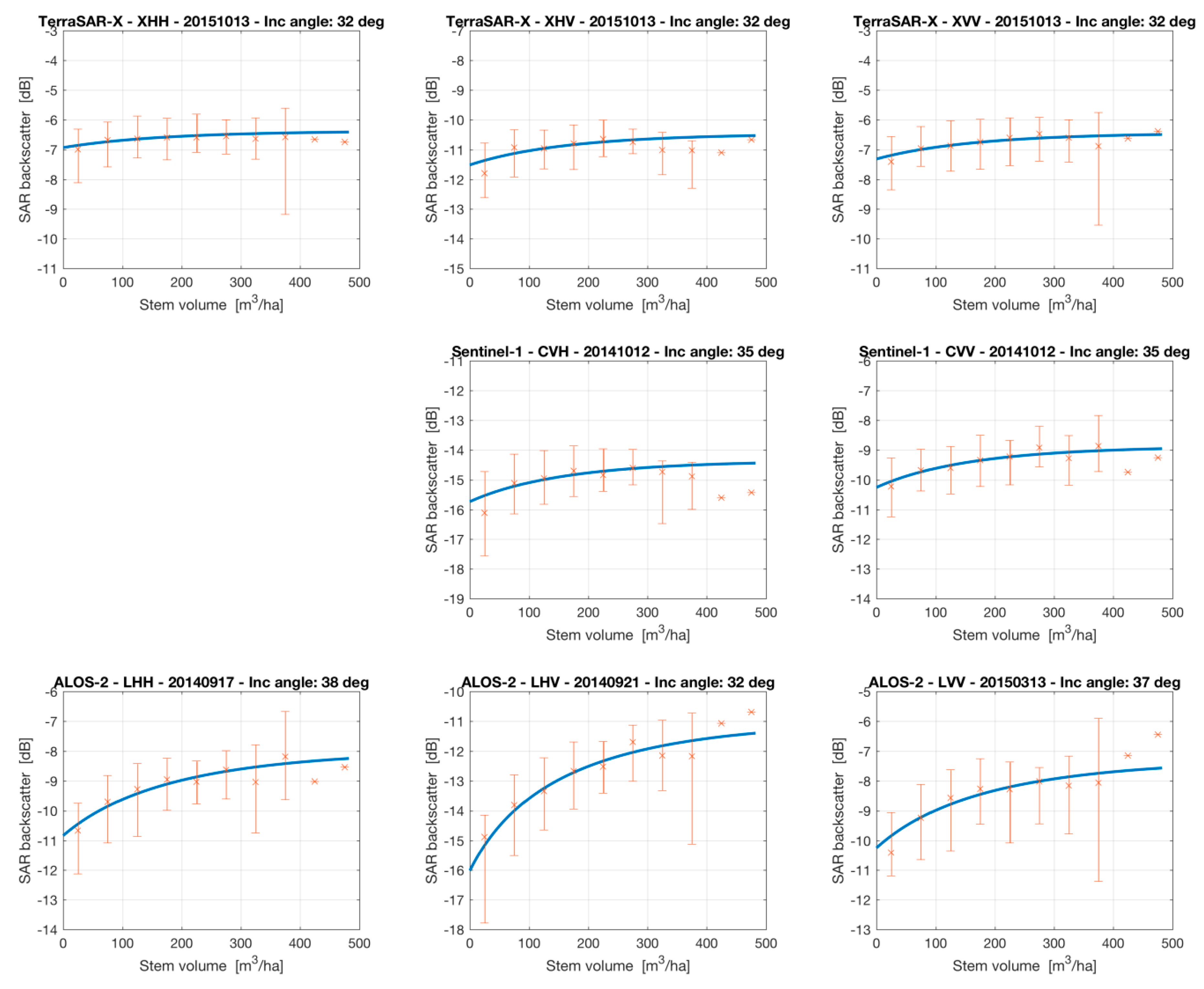
5.1. Signatures of Forest Backscatter as a Function of Stem Volume
5.2. Estimates of the WCM Parameters
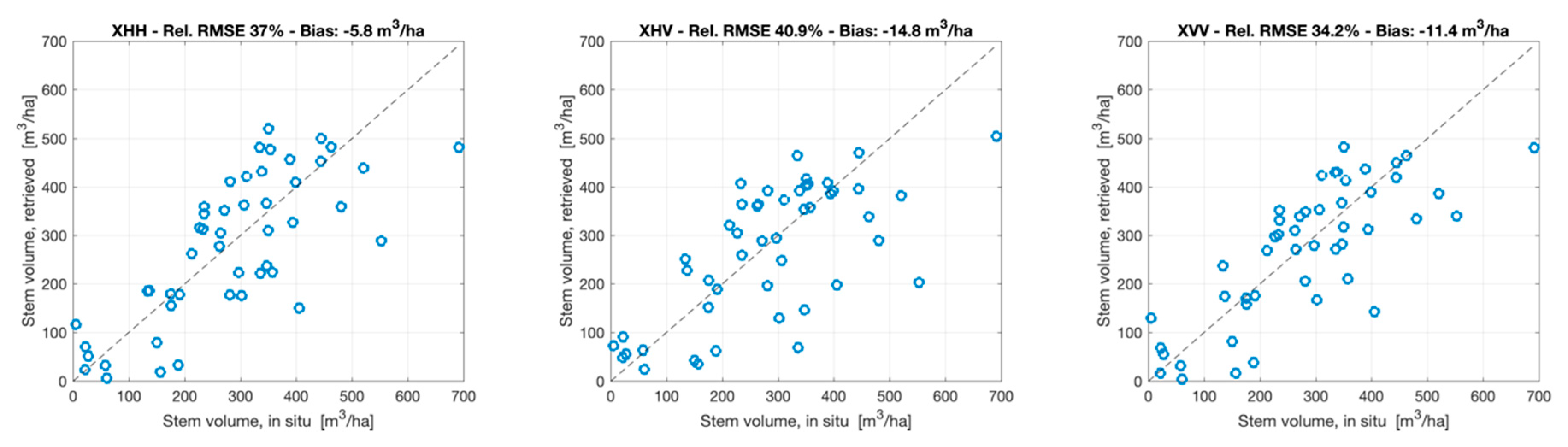
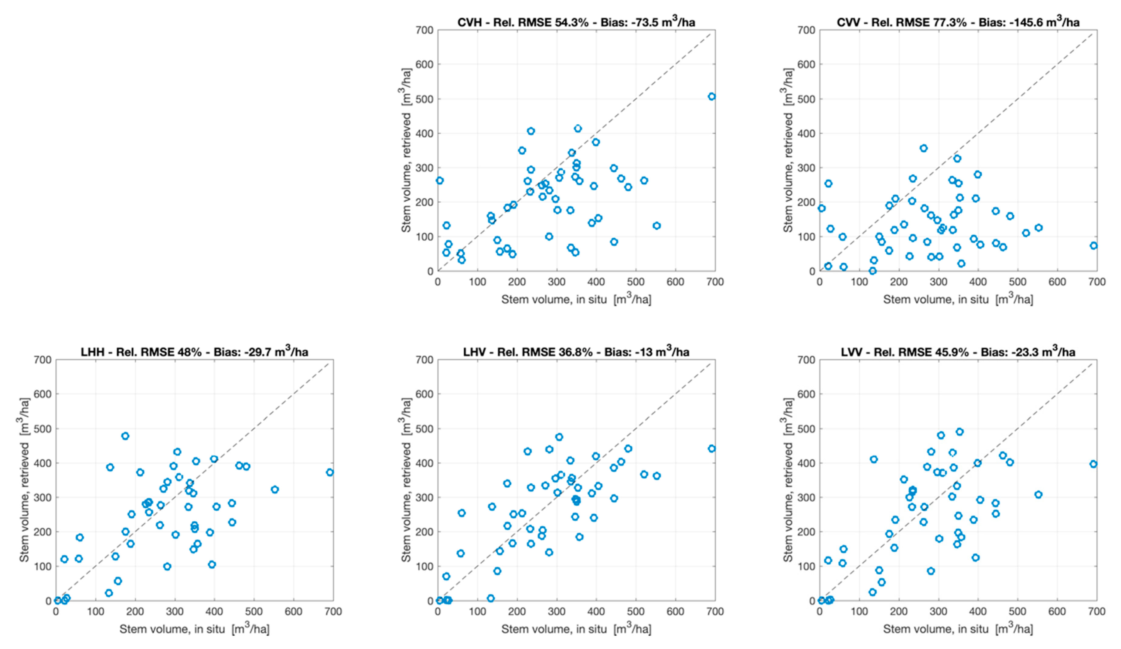
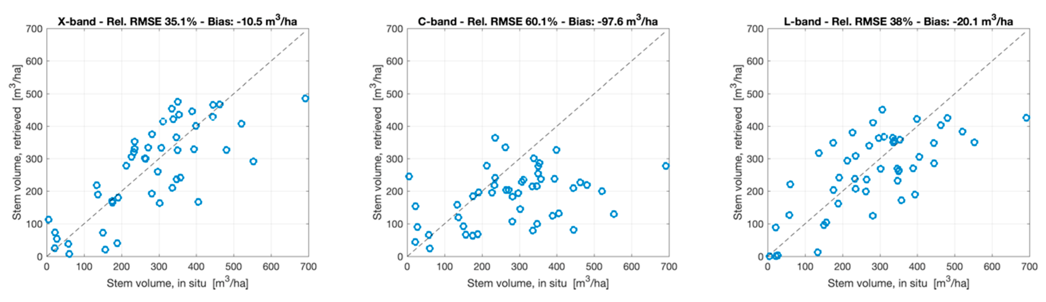
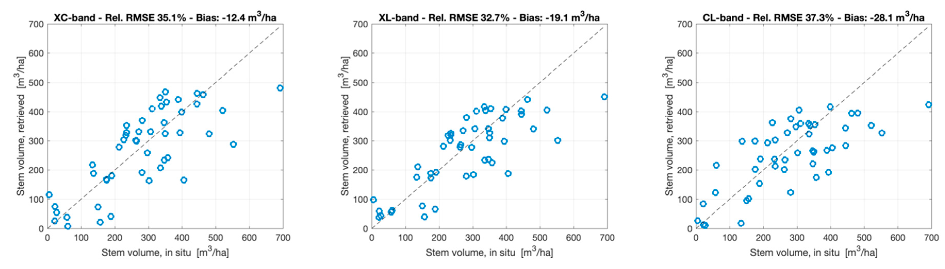
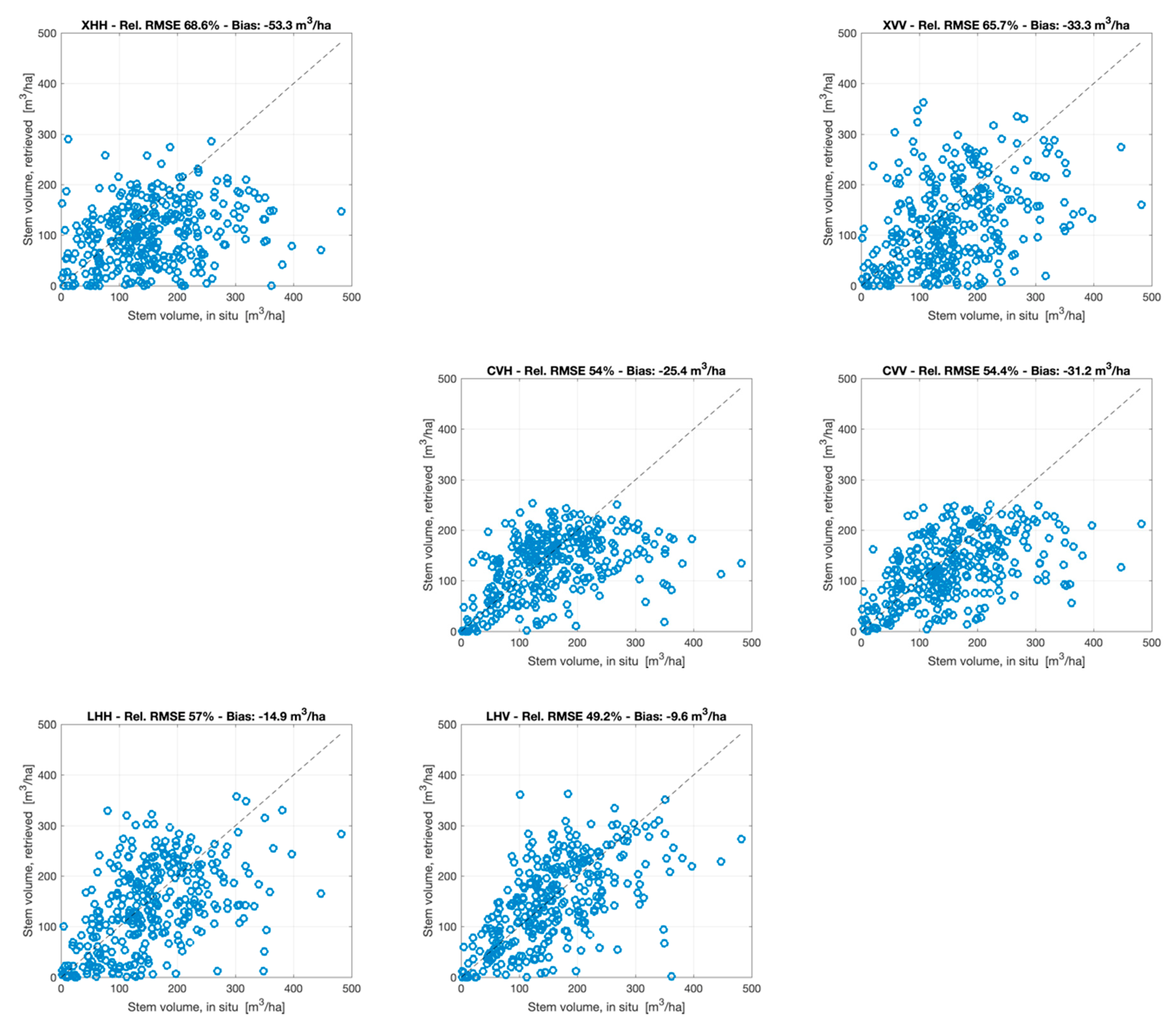
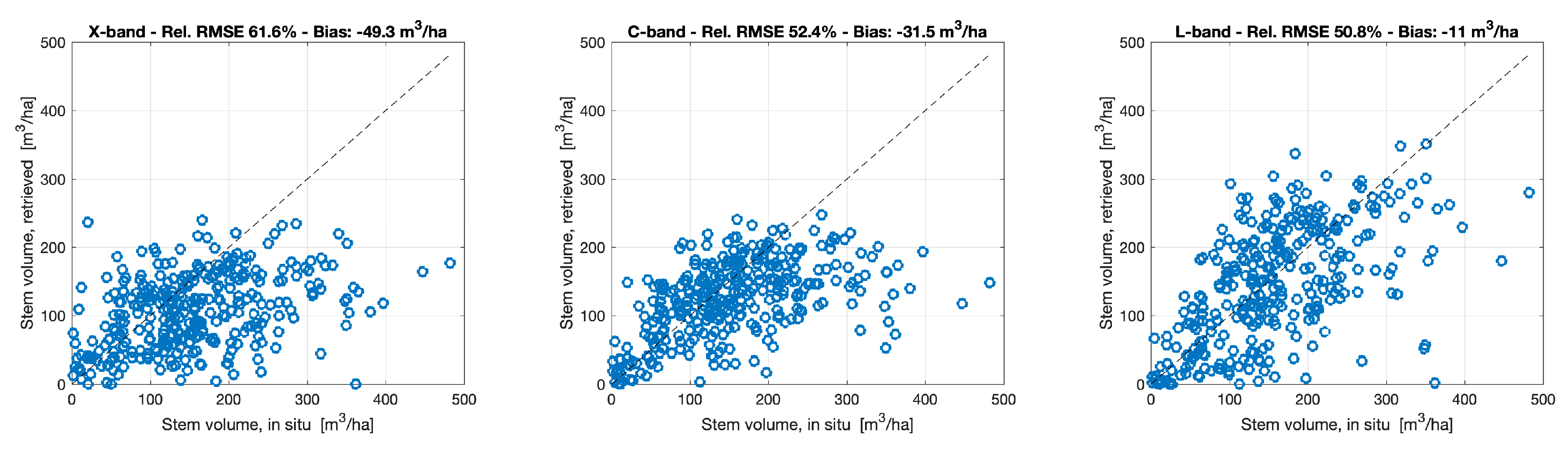
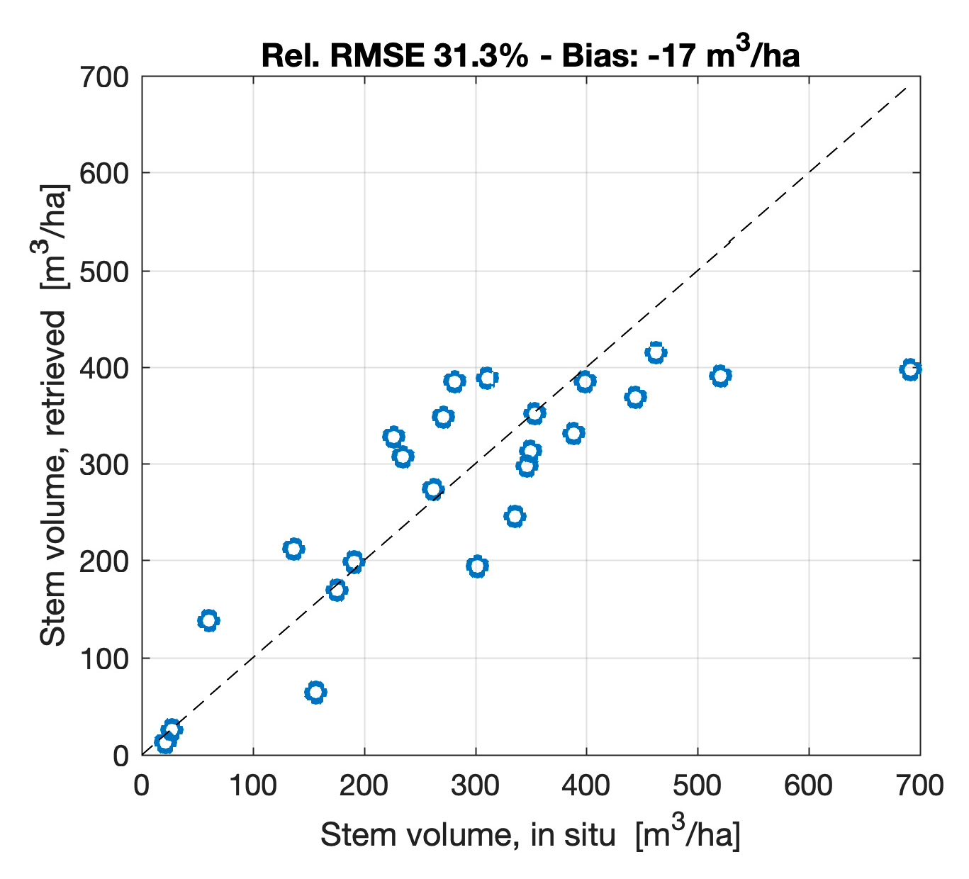
5.3. Retrieval of Stem Volume Using Single and Multiple Observations
- Single frequency band, single polarization, multi-temporal data (MT combination),
- Single frequency band, multi-polarized and multi-temporal data (MTP combination),
- Multiple frequency bands, multi-polarization and multi-temporal data (MTPF combination).
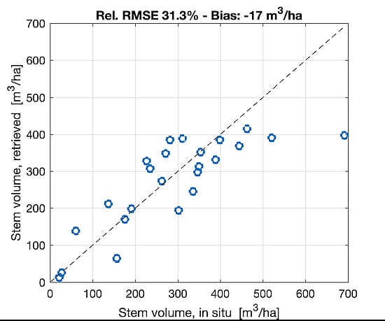
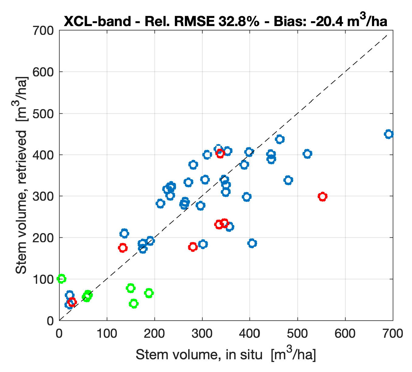
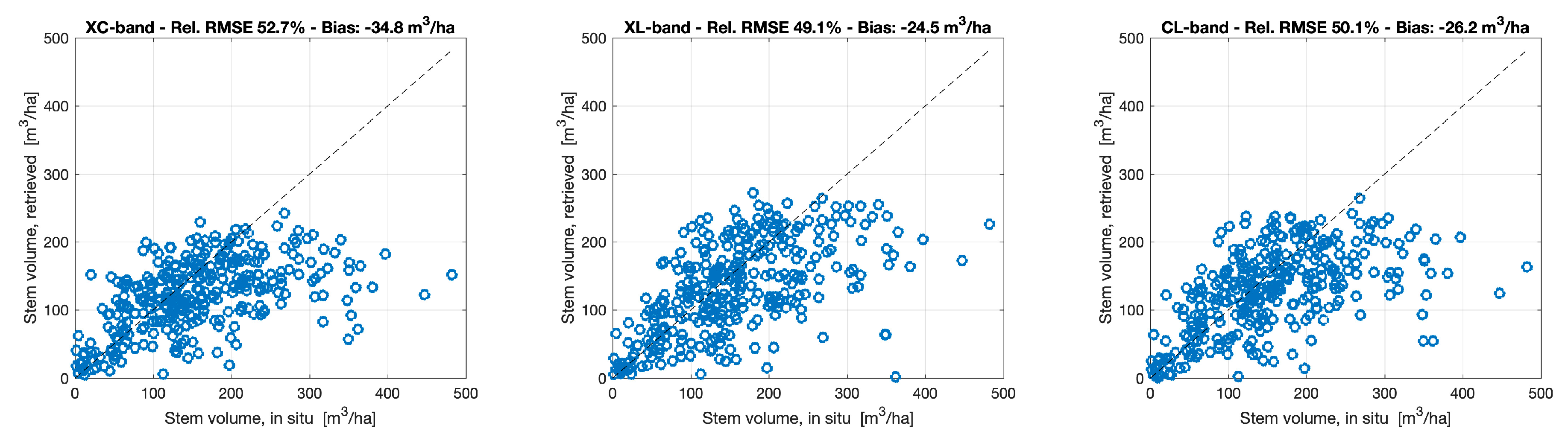
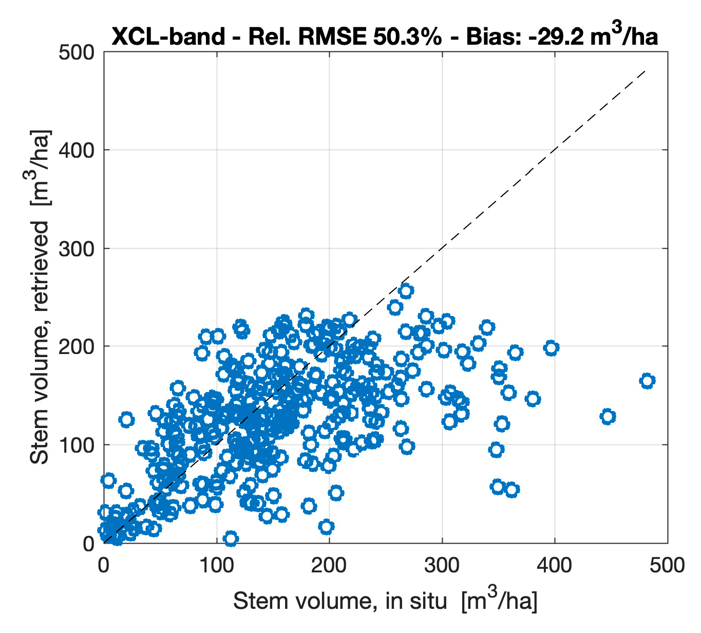
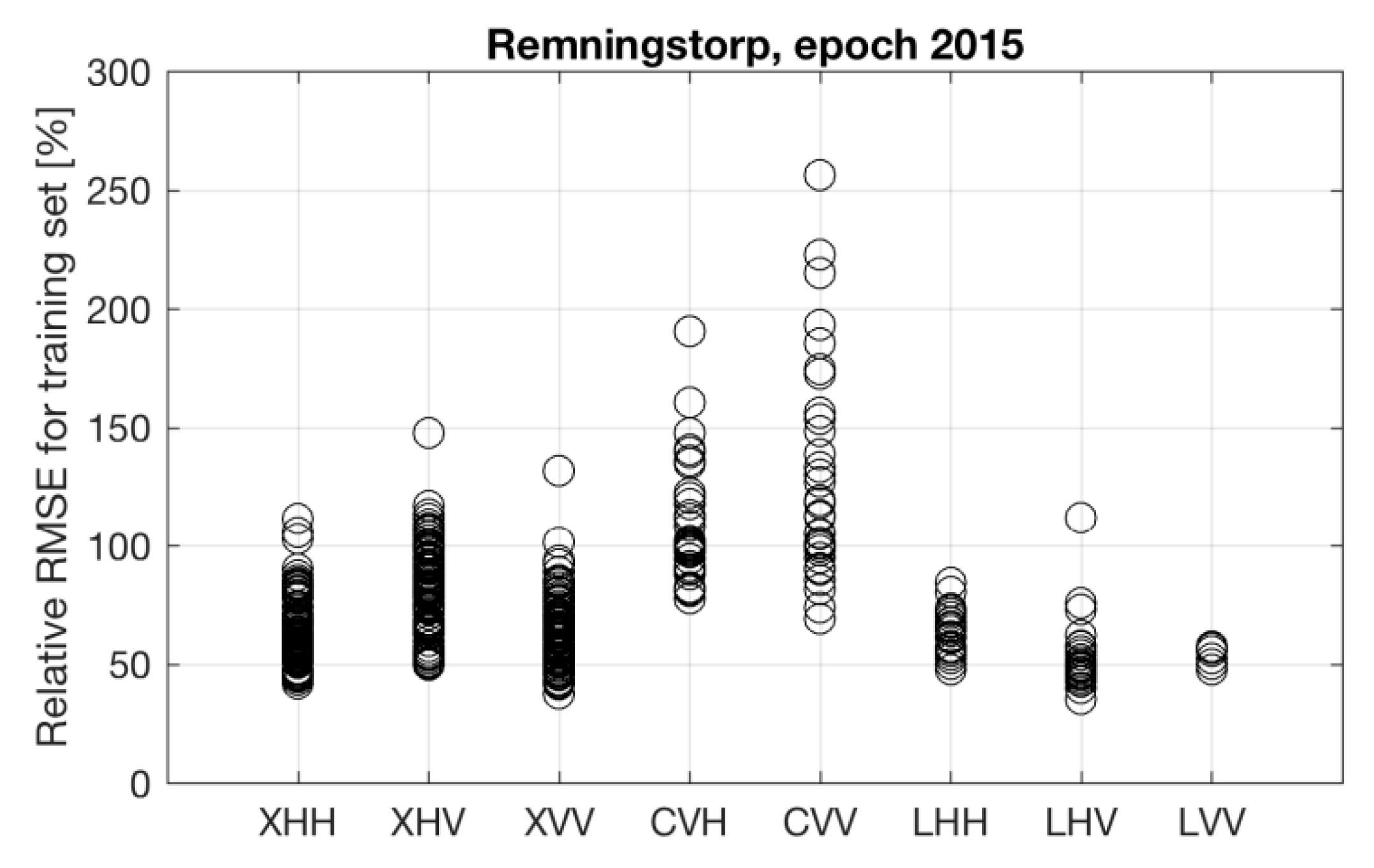
5.4. Assessing the Multi-Frequency Retrieval of Stem Volume
6. Discussion
7. Conclusions
Supplementary Materials
Author Contributions
Funding
Acknowledgments
Conflicts of Interest
References
- Houghton, R.A. Aboveground Forest Biomass and the Global Carbon Balance. Glob. Chang. Biol. 2005, 11, 945–958. [Google Scholar] [CrossRef]
- Le Quéré, C.; Andrew, R.M.; Friedlingstein, P.; Sitch, S.; Pongratz, J.; Manning, A.C.; Korsbakken, J.I.; Peters, G.P.; Canadell, J.G.; Jackson, R.B.; et al. Global Carbon Budget 2017. Earth Syst. Sci. Data 2018, 10, 405–448. [Google Scholar] [CrossRef] [Green Version]
- Santoro, M.; Cartus, O. Research pathways of forest above-ground biomass estimation based on SAR backscatter and interferometric SAR observations. Remote Sens. 2018, 10, 608. [Google Scholar] [CrossRef]
- Lavalle, M.; Hensley, S. Extraction of Structural and Dynamic Properties of Forests from Polarimetric-Interferometric SAR Data Affected by Temporal Decorrelation. IEEE Trans. Geosci. Remote Sens. 2015, 53, 4752–4767. [Google Scholar] [CrossRef]
- Kurvonen, L.; Pulliainen, J.; Hallikainen, M. Retrieval of biomass in boreal forests from multitemporal ERS-1 and JERS-1 SAR images. IEEE Trans. Geosci. Remote Sens. 1999, 37, 198–205. [Google Scholar] [CrossRef] [Green Version]
- Santoro, M.; Beer, C.; Cartus, O.; Schmullius, C.; Shvidenko, A.; McCallum, I.; Wegmüller, U.; Wiesmann, A. Retrieval of growing stock volume in boreal forest using hyper-temporal series of Envisat ASAR ScanSAR backscatter measurements. Remote Sens. Environ. 2011, 115, 490–507. [Google Scholar] [CrossRef]
- Santoro, M.; Eriksson, L.E.B.; Fransson, J.E.S. Reviewing ALOS PALSAR backscatter observations for stem volume retrieval in Swedish forest. Remote Sens. 2015, 7, 4290–4317. [Google Scholar] [CrossRef]
- Ranson, K.J.; Sun, G. Mapping biomass of a northern forest using multifrequency SAR data. IEEE Trans. Geosci. Remote Sens. 1994, 32, 388–396. [Google Scholar] [CrossRef]
- Ranson, K.J.; Sun, G. An evaluation of AIRSAR and SIR-C/X-SAR images for mapping northern forest attributes in Maine, USA. Remote Sens. Environ. 1997, 59, 203–222. [Google Scholar] [CrossRef]
- Pairman, D.; McNeill, S.; Scott, N.; Belliss, S. Vegetation identification and biomass estimation using Airsar data. Geocarto Int. 1999, 14, 69–77. [Google Scholar] [CrossRef]
- Lucas, R.M.; Cronin, N.; Lee, A.; Moghaddam, M.; Witte, C.; Tickle, P. Empirical relationships between AIRSAR backscatter and LiDAR-derived forest biomass, Queensland, Australia. Remote Sens. Environ. 2006, 100, 407–425. [Google Scholar] [CrossRef]
- Saatchi, S.; Halligan, K.; Despain, D.G.; Crabtree, R.L. Estimation of forest fuel load from radar remote sensing. IEEE Trans. Geosci. Remote Sens. 2007, 45, 1726–1740. [Google Scholar] [CrossRef]
- Cartus, O.; Santoro, M.; Wegmüller, U.; Rommen, B. Exploring the capabilities of C-,L- and P-band SAR to estimate aboveground biomass of boreal forests. submitted.
- Krieger, G.; Moreira, A.; Fiedler, H.; Hajnsek, I.; Werner, M.; Younis, M.; Zink, M. TanDEM-X: a satellite formation for high-resolution SAR interferometry. IEEE Trans. Geosci. Remote Sens. 2007, 45, 3317–3341. [Google Scholar] [CrossRef]
- Torres, R.; Snoeij, P.; Geudtner, D.; Bibby, D.; Davidson, M.; Attema, E.; Potin, P.; Rommen, B.; Floury, N.; Brown, M.; et al. GMES Sentinel-1 mission. Remote Sens. Environ. 2012, 120, 9–24. [Google Scholar] [CrossRef]
- Rosenqvist, A.; Shimada, M.; Ito, N.; Watanabe, M. ALOS PALSAR: A Pathfinder Mission for Global-Scale Monitoring of the Environment. IEEE Trans. Geosci. Remote Sens. 2007, 45, 3307–3316. [Google Scholar] [CrossRef]
- Le Toan, T.; Quegan, S.; Davidson, M.W.J.; Balzter, H.; Paillou, P.; Papathanassiou, K.; Plummer, S.; Rocca, F.; Saatchi, S.; Shugart, H.; et al. The BIOMASS mission: Mapping global forest biomass to better understand the terrestrial carbon cycle. Remote Sens. Environ. 2011, 115, 2850–2860. [Google Scholar] [CrossRef] [Green Version]
- Sandberg, G.; Ulander, L.M.H.; Fransson, J.E.S.; Holmgren, J.; Le Toan, T. L- and P-band backscatter intensity for biomass retrieval in hemiboreal forest. Remote Sens. Environ. 2011, 115, 2874–2886. [Google Scholar] [CrossRef]
- Soja, M.J.; Sandberg, G.; Ulander, L.M.H. Regression-based retrieval of boreal forest biomass in sloping terrain using P-band SAR backscatter intensity data. IEEE Trans. Geosci. Remote Sens. 2013, 51, 2646–2665. [Google Scholar] [CrossRef]
- Askne, J.I.A.; Fransson, J.E.S.; Santoro, M.; Soja, M.J.; Ulander, L.M.H. Model-based biomass estimation of a hemi-boreal forest from multitemporal TanDEM-X acquisitions. Remote Sens. 2013, 5, 5574–5597. [Google Scholar] [CrossRef]
- Persson, H.; Fransson, J.E.S. Forest variable estimation using radargrammetric processing of TerraSAR-X images in boreal forests. Remote Sens. 2014, 6, 2084–2107. [Google Scholar] [CrossRef]
- Persson, H.J.; Fransson, J.E.S. Comparison between TanDEM-X- and ALS-based estimation of aboveground biomass and tree height in boreal forests. Scand. J. For. Res. 2017, 32, 306–319. [Google Scholar] [CrossRef]
- IPCC. 2006 IPCC Guidelines for National Greenhouse Gas Inventories, Volume 4: Agriculture, Forestry and Other Land Use. 2006. Available online: https://www.ipcc-nggip.iges.or.jp/public/2006gl/vol4.html (accessed on 28 May 2019).
- Soja, M.J.; Askne, J.I.H.; Ulander, L.M.H. Estimation of Boreal Forest Properties from TanDEM-X Data Using Inversion of the Interferometric Water Cloud Model. IEEE Geosci. Remote Sens. Lett. 2017, 14, 997–1001. [Google Scholar] [CrossRef]
- Werner, C.; Wegmüller, U.; Strozzi, T.; Wiesmann, A. GAMMA SAR and interferometric processing software. In Proceedings of the ERS-Envisat Symposium, Gothenburg, Sweden, 16–20 October 2000; p. CD-ROM. [Google Scholar]
- Oliver, C.; Quegan, S. Understanding Synthetic Aperture Radar Images; Artech House: Boston, MA, USA, 1998. [Google Scholar]
- Wegmüller, U. Automated terrain corrected SAR geocoding. In Proceedings of the IGARSS’99, Hamburg, Germany, 28 June–2 July 1999; IEEE Publications: Piscataway, NJ, USA, 1999; pp. 1712–1714. [Google Scholar]
- Frey, O.; Santoro, M.; Werner, C.; Wegmüller, U. DEM-based SAR pixel-area estimation for enhanced geocoding refinement and radiometric normalization. IEEE Geosci. Remote Sens. Lett. 2013, 10, 48–52. [Google Scholar] [CrossRef]
- Quegan, S.; Yu, J.J. Filtering of multichannel SAR images. IEEE Trans. Geosci. Remote Sens. 2001, 39, 2373–2379. [Google Scholar] [CrossRef]
- Lopes, A.; Nezry, E.; Touzi, R.; Laur, H. Structure detection and statistical adaptive speckle filtering in SAR images. Int. J. Remote Sens. 1993, 14, 1735–1758. [Google Scholar] [CrossRef]
- Santoro, M.; Fransson, J.E.S.; Eriksson, L.E.B.; Magnusson, M.; Ulander, L.M.H.; Olsson, H. Signatures of ALOS PALSAR L-band backscatter in Swedish forest. IEEE Trans. Geosci. Remote Sens. 2009, 47, 4001–4019. [Google Scholar] [CrossRef]
- Askne, J.; Dammert, P.B.G.; Ulander, L.M.H.; Smith, G. C-band repeat-pass interferometric SAR observations of the forest. IEEE Trans. Geosci. Remote Sens. 1997, 35, 25–35. [Google Scholar] [CrossRef]
- Santoro, M.; Askne, J.; Smith, G.; Fransson, J.E.S. Stem volume retrieval in boreal forests with ERS-1/2 interferometry. Remote Sens. Environ. 2002, 81, 19–35. [Google Scholar] [CrossRef]
- Pulliainen, J.T.; Heiska, K.; Hyyppä, J.; Hallikainen, M.T. Backscattering properties of boreal forests at the C- and X-bands. IEEE Trans. Geosci. Remote Sens. 1994, 32, 1041–1050. [Google Scholar] [CrossRef]
- Monteith, A.R.; Ulander, L.M.H. Temporal survey of P- and L-band polarimetric backscatter in boreal forests. IEEE J. Sel. Top. Appl. Earth Obser. Remote Sens. 2018, 11, 3564–3577. [Google Scholar] [CrossRef]
- Folkesson, K.; Smith-Jonforsen, G.; Ulander, L.M.H. Validating backscatter models for CARABAS SAR images of coniferous forests. Canad. J. Remote Sens. 2008, 34, 480–495. [Google Scholar] [CrossRef]


| Band | Sensor | Polarization | Look Angle | Data Sets | Time Interval |
|---|---|---|---|---|---|
| X | TerraSAR-X | Single-pol (HH or VV) | 22°–51° | 62 | 201410–201510 |
| C | Sentinel-1A | Dual-pol (VV, VH) | 39° | 33 | 201410–201510 |
| L | ALOS-2 PALSAR-2 | Dual pol (HH, HV) Full pol. (HH, HV, VV) | 28°–36° | 24 | 201409–201510 |
| Band | Sensor | Polarization | Look Angle | Data Sets | Time Interval |
|---|---|---|---|---|---|
| X | TerraSAR-X | Single-pol (HH or VV) | 19°–48° | 21 | 201407–201510 |
| C | Sentinel-1A | Dual-pol (VV, VH) | 39° | 78 | 201410–201510 |
| L | ALOS-2 PALSAR-2 | Dual pol (HH, HV) Full pol. (HH, HV, VV) | 28°–36° | 15 | 201408–201510 |
| Sensor | ENL After Multi-Looking | ENL After Multi-Channel Filtering |
|---|---|---|
| TerraSAR-X | 12 | 168 |
| Sentinel-1 | 5 | 40 |
| ALOS-2 PALSAR-2 | 10 | 20 |
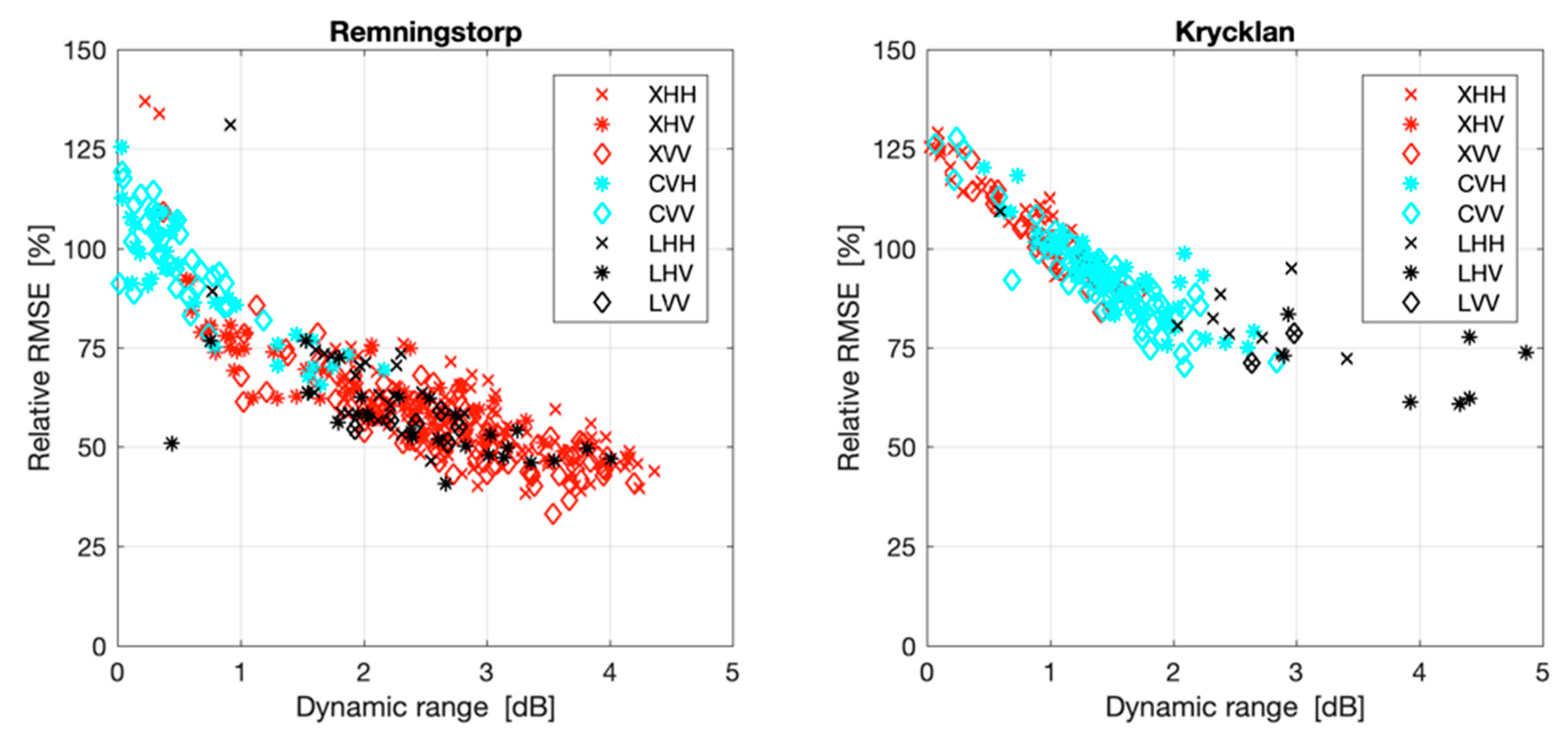
| Sensor | Band-Polarization | Trend Backscatter vs. Stem Volume | Dynamic Range | Rel. RMSE |
|---|---|---|---|---|
| TerraSAR-X | XHH | Decreasing | 3–4 dB | ~50% |
| TerraSAR-X | XHV | Decreasing | 1–4 dB (*) | ≥50% |
| TerraSAR-X | XVV | Decreasing | 3–4 dB | ~50% |
| Sentinel-1 | CVH | Decreasing | 0–2 dB (*) | ~70–100% |
| Sentinel-1 | CVV | Decreasing | 0–1 dB (*) | ~90–110% |
| ALOS-2 | LHH | Increasing | 1–2 dB (**) | ~50–60% |
| ALOS-2 | LVV | Increasing | 2–3 dB (**) | ~50–60% |
| (*) larger dynamic range under frozen conditions (i.e., min temperature below 0 °C) (**) larger dynamic range under unfrozen conditions (i.e., min temperature above 0 °C) | ||||
| Sensor | Band-Polarization | Trend backscatter vs. Stem Volume | Dynamic Range | Rel. RMSE |
|---|---|---|---|---|
| TerraSAR-X | XHH | Decreasing/constant | <1 dB (*) | ~110% |
| TerraSAR-X | XVV | Increasing | 1 dB | ~95% |
| Sentinel-1 | CVH | Increasing | ~1 dB | 80–100% |
| Sentinel-1 | CVV | Increasing | ~1 dB | 80–100% |
| ALOS-2 | CHH | Increasing | 3 dB | ~60% |
| ALOS-2 | CHV | Increasing | 5 dB | 50–70% |
| (*) larger dynamic range under steep look angles (< 20°) (**) larger dynamics range under unfrozen conditions (i.e., min temperature above 0°C) | ||||
| Band | Sensor | Test Sites | Reference Data | Remarks | Reference |
|---|---|---|---|---|---|
| L | ALOS PALSAR | Remningstorp and Krycklan | Hectare-scale stands | Multi-temporal dataset RMSE: 35% and 44%. | [7] |
| L | E-SAR | Remningstorp | Sub hectare-scale stands Laser scanning data and 10- radius inventory plots | Single-image retrieval RMSE: 31–46% | [18] |
| P | E-SAR | Remningstorp | Sub hectare-scale stands Laser scanning data and 10- radius inventory plots | Single-image retrieval RMSE: 18–27% | [18] |
| P | E-SAR | Remningstorp and Krycklan | Hectare-scale stands | RMSE: 28–42% at Krycklan. RMSE of 22–33% using the backscatter model developed at Krycklan | [19] |
| VHF | CARABAS | Remningstorp | Hectare-scale stands | Multiple viewing directions RMSE: 11–25% | [36] |
© 2019 by the authors. Licensee MDPI, Basel, Switzerland. This article is an open access article distributed under the terms and conditions of the Creative Commons Attribution (CC BY) license (http://creativecommons.org/licenses/by/4.0/).
Share and Cite
Santoro, M.; Cartus, O.; Fransson, J.E.S.; Wegmüller, U. Complementarity of X-, C-, and L-band SAR Backscatter Observations to Retrieve Forest Stem Volume in Boreal Forest. Remote Sens. 2019, 11, 1563. https://0-doi-org.brum.beds.ac.uk/10.3390/rs11131563
Santoro M, Cartus O, Fransson JES, Wegmüller U. Complementarity of X-, C-, and L-band SAR Backscatter Observations to Retrieve Forest Stem Volume in Boreal Forest. Remote Sensing. 2019; 11(13):1563. https://0-doi-org.brum.beds.ac.uk/10.3390/rs11131563
Chicago/Turabian StyleSantoro, Maurizio, Oliver Cartus, Johan E. S. Fransson, and Urs Wegmüller. 2019. "Complementarity of X-, C-, and L-band SAR Backscatter Observations to Retrieve Forest Stem Volume in Boreal Forest" Remote Sensing 11, no. 13: 1563. https://0-doi-org.brum.beds.ac.uk/10.3390/rs11131563