On the Sensitivity of TanDEM-X-Observations to Boreal Forest Structure


1
Department of Space, Earth and Environment, Chalmers University of Technology, SE-412 96 Gothenburg, Sweden
2
Department of Forest Resource Management, Swedish University of Agricultural Sciences, SE-901 83 Umeå, Sweden
*
Author to whom correspondence should be addressed.
Remote Sens. 2019, 11(14), 1644; https://0-doi-org.brum.beds.ac.uk/10.3390/rs11141644
Submission received: 7 May 2019
/
Revised: 27 June 2019
/
Accepted: 4 July 2019
/
Published: 10 July 2019
(This article belongs to the Special Issue Remote Sensing of Boreal Forests)
Abstract
:The structure of forests is important to observe for understanding coupling to global dynamics of ecosystems, biodiversity, and management aspects. In this paper, the sensitivity of X-band to boreal forest stem volume and to vertical and horizontal structure in the form of forest height and horizontal vegetation density is studied using TanDEM-X satellite observations from two study sites in Sweden: Remningstorp and Krycklan. The forest was analyzed with the Interferometric Water Cloud Model (IWCM), without the use of local data for model training, and compared with measurements by Airborne Lidar Scanning (ALS). On one hand, a large number of stands were studied, and in addition, plots with different types of changes between 2010 and 2014 were also studied. It is shown that the TanDEM-X phase height is, under certain conditions, equal to the product of the ALS quantities for height and density. Therefore, the sensitivity of phase height to relative changes in height and density is the same. For stands with a phase height >5 m we obtained an root-mean-square error, RMSE, of 8% and 10% for tree height in Remningstorp and Krycklan, respectively, and for vegetation density an RMSE of 13% for both. Furthermore, we obtained an RMSE of 17% for estimation of above ground biomass at stand level in Remningstorp and in Krycklan. The forest changes estimated with TanDEM-X/IWCM and ALS are small for all plots except clear cuts but show similar trends. Plots without forest management changes show a mean estimated height growth of 2.7% with TanDEM-X/IWCM versus 2.1% with ALS and a biomass growth of 4.3% versus 4.2% per year. The agreement between the estimates from TanDEM-X/IWCM and ALS is in general good, except for stands with low phase height.

1. Introduction
Remote sensing methods to determine forest properties such as above ground biomass (AGB) and forest structure such as height and vegetation density are important, cf. [1] (In this paper, the word vegetation density will be used to describe the horizontal vegetation density as measured either by airborne lidar scanning, ALS, or TanDEM-X.) AGB has been identified as an Essential Climate Variable, needed to reduce uncertainties in our knowledge of the climate system [2] and the structure is important for management aspects and biodiversity. Thirty percent of the forested area in the world consists of boreal forests, and in Sweden, 51% of the land area is covered by productive forest of mainly boreal or hemi-boreal types. The boreal forests are characterized by long winter conditions with freezing and snow cover and are mostly dominated by coniferous species. The forest structure is influenced by growth, mortality, and degradation as well as management conditions.
X-band data in the form of bistatic TanDEM-X observations have recently been considered as possible to use for stem volume or AGB estimation in boreal forests [3,4,5,6,7,8,9,10,11,12] as well as tropical forests [13,14,15,16,17,18]. In particular, in the case of boreal forest, high accuracy estimates of AGB have been obtained. X-band had earlier been assumed not to be useful for forest applications due to a low penetration into the forest. Instead, low frequency has been seen as the promising alternative due to its high penetration into the forest and sensitivity to the more important part of the forest contributing to AGB such as branches and stems. This conclusion goes back to observations of radar backscatter investigations, e.g., [19,20,21]. However, with interferometric synthetic aperture radar, InSAR, using the coherent combination of two SAR observations, phase and coherence could be observed in addition to backscatter. This increased the information content.
The first reported InSAR observations of boreal forest [22] were based on repeat-pass interferometry. By using observations from ERS-1 in its 3 day repeat-pass cycle it was concluded that “Interferometric phase measurements show that the scattering at C-band is close to the tree top when the forest is dense, otherwise it is related to the height and density of trees.“ The analysis was continued in [23,24,25]. A major obstacle in the analysis was the additional uncertainty due to temporal decorrelation related to the time lag between the two observations and the associated changes of the forest due to wind effects for example. Coherence and backscatter were the major data, while the scattering phase center height (simply denoted phase height below) was found to be unstable [26].
The Shuttle Radar Topography Mission (SRTM) in 2000, covered latitudes up to 60° N with a C- and X-band transmitter and two receivers separated by a 60 m long boom. It offered the first possibility in space to analyze InSAR without temporal decorrelation [27]. A study showed high correlation between the SRTM phase height and canopy height, and investigated the ability of X-band phase height for estimation of key forest monitoring variables, namely height, stand density, stem volume, and AGB [28].
TanDEM-X was launched in 2010 as a twin satellite to TerraSAR-X and offered for the first time bistatic InSAR observations, with two satellites observing the same area near simultaneously [29]. This resulted in observations with negligible temporal decorrelation and made accurate phase height observations possible. With a known digital terrain model (DTM), a reference level for the scattering phase center was estimated. The resulting phase height was shown to be closely related to the forest height and the stem volume or AGB. A small penetration at X-band is an advantage instead of a disadvantage with this technique, when the forest height is closely related to stem volume or AGB. However, interest has not only been focused on stem volume or AGB but also on the sensitivity for other properties such as height and density [12,13,28,30,31,32,33,34,35,36,37,38,39,40].
The goal of this paper is to study the estimation of horizontal and vertical forest properties, such as vegetation density and height, as well as stem volume. The investigation will be based on complementary studies: on one hand using a large number of stands in order to evaluate more general aspects and on the other hand 4 × 12 plots with different changes in order to analyze specific aspects. Forest properties in Remningstorp and Krycklan were studied by means of bistatic TanDEM-X data and a DTM using the Interferometric Water Cloud Model (IWCM), without the use of local training data.
The study sites and the measurements are presented first. The model for interpretation is introduced and results for height, density, and stem volume are compared with ALS observations and some general aspects studied. The plots with changes are illustrating the sensitivity of TanDEM-X to forest properties related to forest management changes. Finally, the results are discussed including the use of TanDEM-X as an alternative to ALS and conclusions are drawn.
2. Study Sites
Remningstorp and Krycklan are two forest sites in Sweden with extensive field studies and with different characteristics.
The study site Remningstorp (Lat 58°30′ N, Long 13°40′ E) is an estate with 1200 hectares (ha) of productive forest area in the hemi-boreal zone. The forest consists mainly of Norway spruce (Picea abies (L.) Karst.), Scots pine (Pinus sylvestris L.), and birch (Betula spp.). The test site is fairly flat with elevations ranging from 120 m to 145 m above sea level, and it is managed by a single owner.
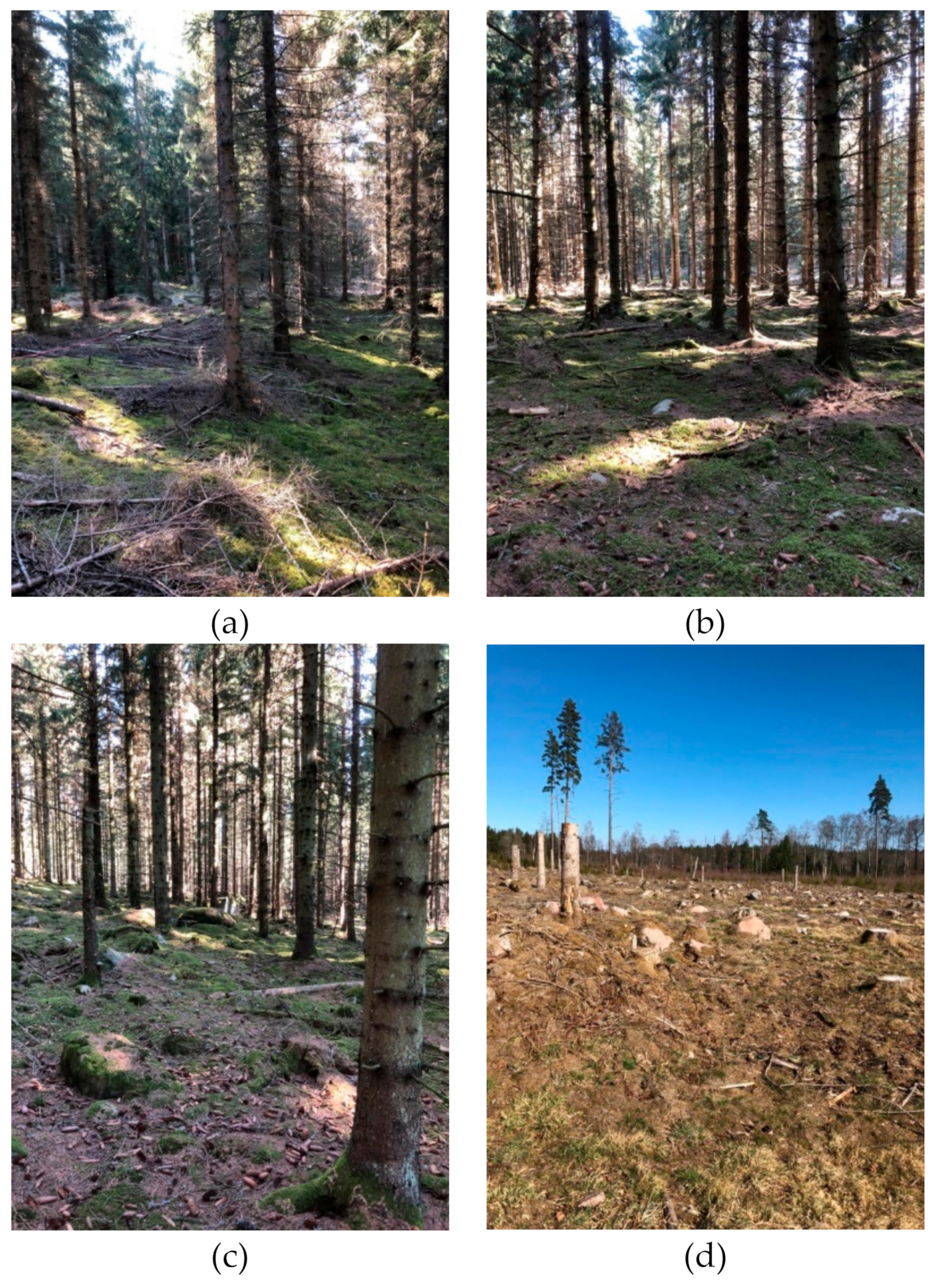
Photographs of some plots in Remningstorp are illustrated in Figure 1.
The study site Krycklan (Lat 64°16′ N Long. 19°46′ E) is a river catchment in northern Sweden and covers approximately 68 km2. The forest consists mainly of Norway spruce (Picea abies (L.) Karst.), Scots pine (Pinus sylvestris L.), and birch (Betula spp.). It is a topographic area with ground elevation varying between 145 m and 400 m above sea level. Slopes measured on a 50 m × 50 m grid varied up to 19° but are locally much steeper, e.g., along the river gorges. Within the area, we analyzed 242 forest stands managed by many different owners and with areas larger than 4 ha.
These two sites have been used as reference sites for remote sensing of boreal forest many times and the sites have then been described in detail in many publications, e.g., [4,10,12,33,41,42,43,44,45,46,47].
The two areas, that are more than 700 km apart, have different characteristics since one is boreal and managed by many different owners (Krycklan) and the other hemi-boreal and managed by a single owner, and the sites have different topography.
3. Data
In this section information about the ALS and TanDEM-X data and the stands and plots selected for the investigation is given. In addition, some properties of the data are illustrated.
3.1. ALS and In Situ Data
Extensive in situ and lidar data were collected in Remningstorp as part of BioSAR 2010 [48]. Lidar acquisitions took place on 29 August 2010 (as part of BioSAR 2010), on 21 April 2011 (as part of a national campaign for estimating a DTM), and on 4 August 2014. Within the area, field and ALS observations of 202 forest stands with areas larger than 1 ha are considered in this paper. In addition, 4 × 12 plots in Remningstorp affected by the three most common forest management changes in Sweden were selected for the period 2011 to 2014 based on the forest management register, and in addition, as reference, plots not affected by any registered changes [33]. The classes are described as pre-commercial thinning (lower vegetation removal, often with diameter at breast height <0.07 m), commercial thinning (commonly denoted only thinning, where about 30–35% of the basal-area is removed, but most often the suppressed trees are removed to gain the highest, remaining trees), and clear-cutting (more or less all trees removed but sometimes seed trees are left). The plots with no other changes than natural growth are denoted “untouched”. The locations were selected relatively evenly over the test site in coniferous forest (>50%), approximately in the stand centers and only in stands having room for an at least a 30 m radius circular plot with available in situ data. To establish classes of equal size, 12 stands of respective type were selected (randomly in those cases where more stands were available). The plot size has significant impact on the results, and 30 m circular plots are assumed sufficient to overcome most local deviations noticed in smaller plots (e.g., 10 m radius), which are related to resolution and local forest structure in the TanDEM-X data [10]. The reference values for the 12 plots from each of the four classes were obtained as mean pixel values within each plot from the ALS estimated raster data. ALS estimates are based on a 5 m raster over Remningstorp. The root-mean-square error, RMSE, was 15.9% for the 2010 ALS AGB map and 14.6% for the 2014 ALS AGB map.
Extensive in situ and lidar data were collected in the summer of 2008 in Krycklan as part of BioSAR 2008 [49]. AGB was determined from ALS data with RMSE = 15.9%. To obtain a similar number of stands as in Remningstorp, field and ALS observations of 242 forest stands with areas larger than 4 ha are considered in this paper.
3.2. TanDEM-X Data
We chose one specific TanDEM-X data set from each site, the first available relative to the ALS observations (Table 1). All acquisitions had an incidence angle of 41°. They had a similar height of ambiguity, HoA, i.e., the height corresponding to a phase change of 2π which determines the sensitivity to forest height changes. A third TanDEM-X data set over Remningstorp in 2014, and close in time to the third ALS scanning, was analyzed with respect to changes since 2011 in the 4 × 12 plots. The TanDEM-X acquisition conditions for this second acquisition over Remningstorp were almost identical to the first. All three TanDEM-X data sets were acquired in VV, i.e., vertical polarization in the transmitted and received signal. TanDEM-X data were based on 5 × 5 multi-looking and a final pixel size of 10 × 10 m2, and finally averaged over the stands or 30 m circular plots.
3.3. Data Properties
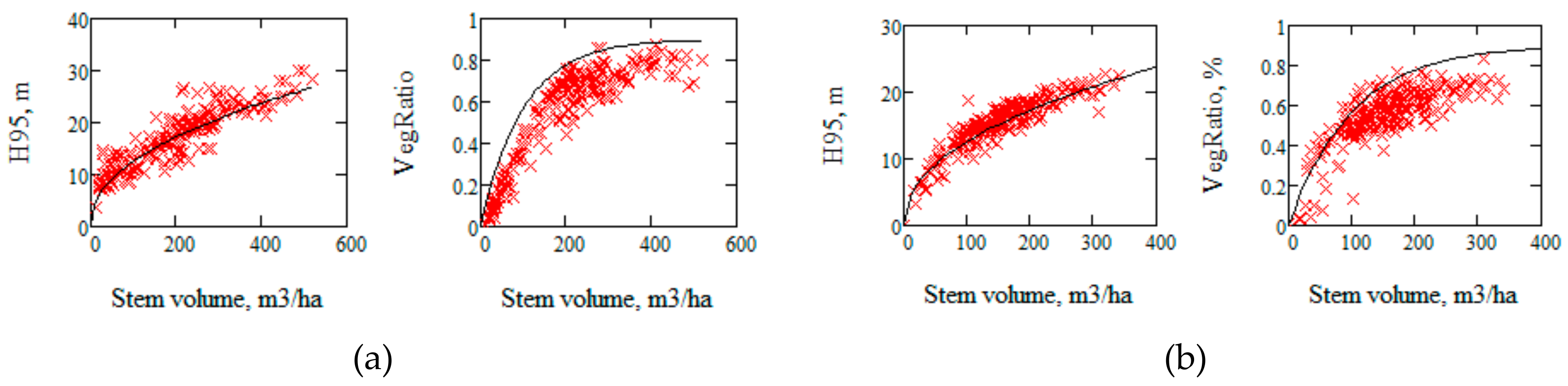
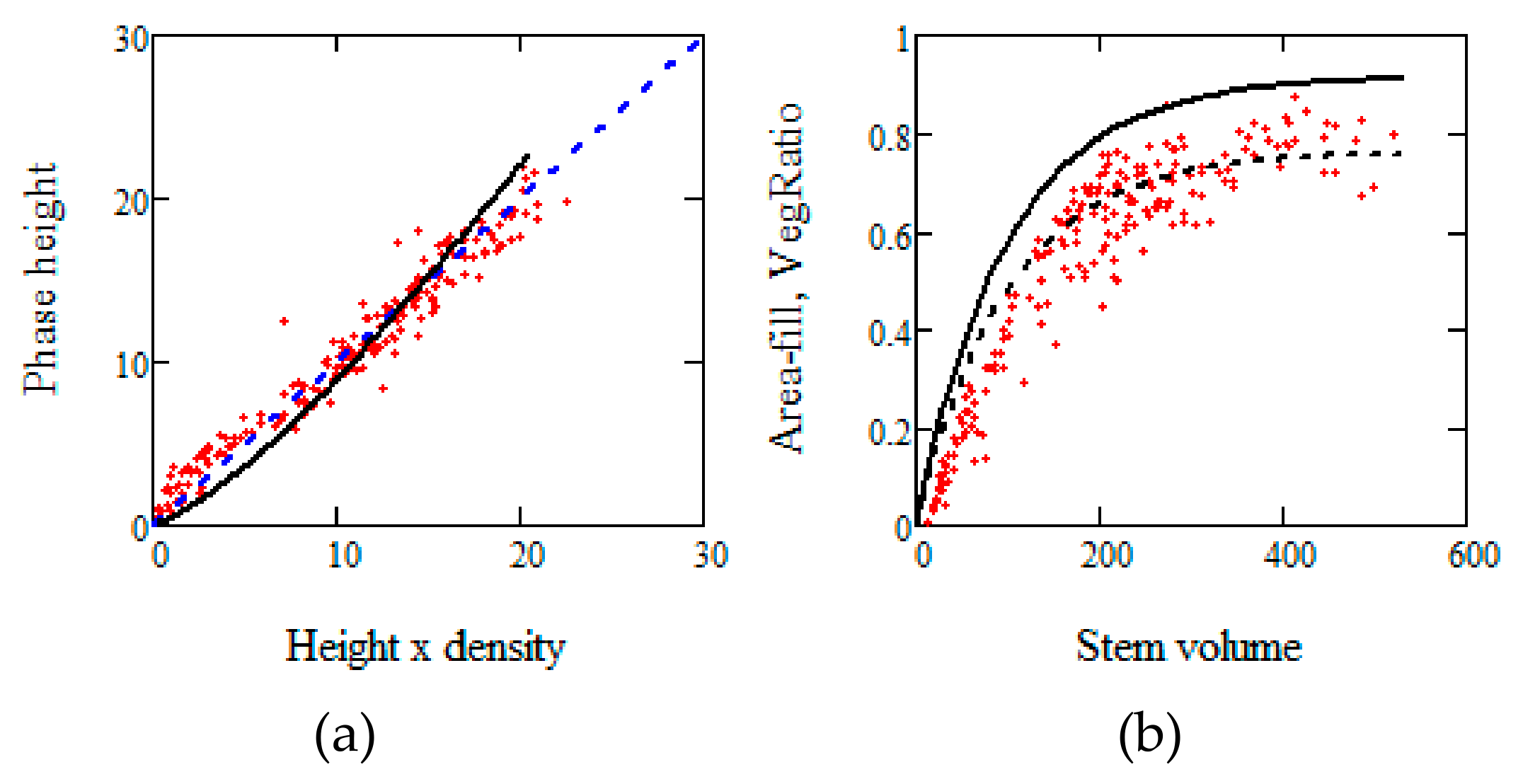
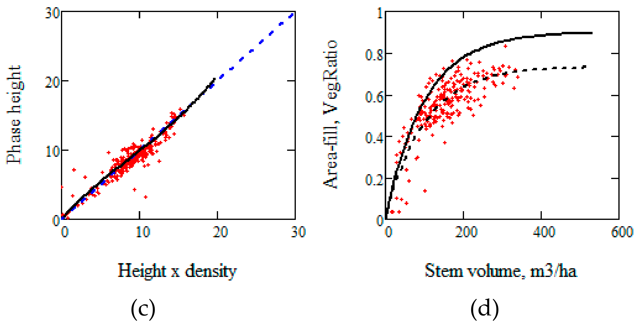
To evaluate the TanDEM-X observations we used the ALS observations of the forest vertical and horizontal structures as characterized by the 95 percentile of the total number of returns, H95, and vegetation ratio as the number of first returns above a 1.37 m threshold in percent of the total number of returns as well as stem volume or AGB. We denote VegRatio = 0.01 vegetation ratio to obtain the fraction of the area covered by vegetation. Stem volume or AGB is estimated by means of regression of ALS observations to the properties of stands with known stem volume or AGB [10,50,51,52]. In Figure 2 these properties are illustrated together with two functions of stem volume, V, to be discussed later, h(V) and η(V).
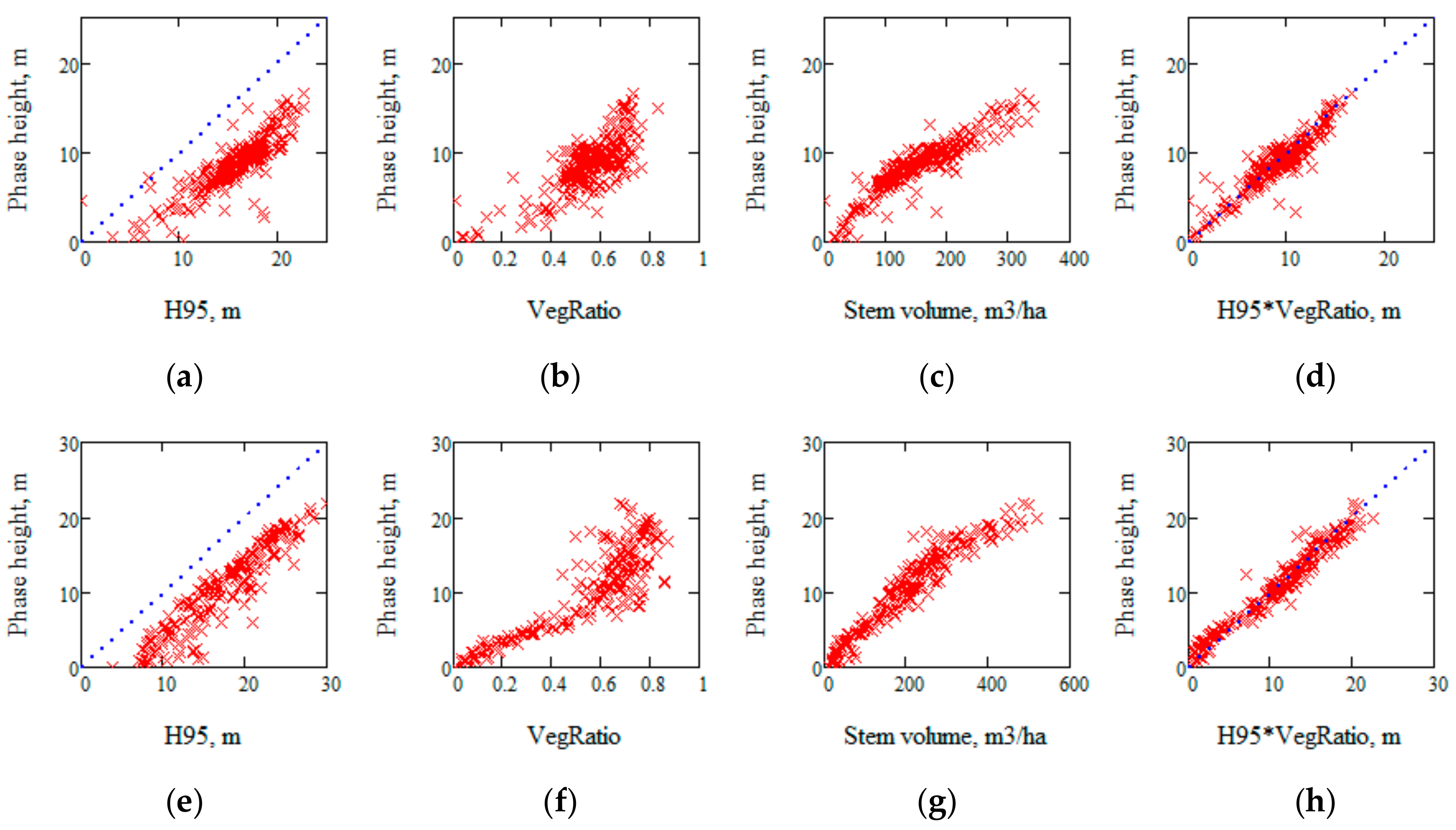
The TanDEM-X interferometric phase was converted to height by HoA and the height difference relative to a lidar DTM is denoted phase height. Figure 3 illustrates the sensitivity of TanDEM-X phase height to properties determined by ALS.
From Figure 3 we see a relatively constant difference between H95 and the phase height, which represents the “penetration depth”, while the relationships between phase height and VegRatio and between phase height and stem volume are quasi-linear. We also see a linear relationship between phase height and the product of H95 and VegRatio.
The primary reference variable in IWCM, used below, is the stem volume, V, and the AGB/stem volume ratio varies in Sweden. For the area investigated in 2014 we have in situ estimates of AGB available and due to the tree-mixture, a mean AGB/stem volume ratio of 0.62 could be determined, which will be used for conversion in conjunction with the 4 × 12 plots.
4. Methods
In this section the method used to interpret the TanDEM-X data is described. IWCM is used to derive properties which can be compared with ALS observations of height, density, and stem volume.
4.1. TanDEM-X Observations Versus ALS Observations
Forest height and density are obvious properties influencing InSAR observations, see Figure 3. Any model of the scattering from the complex structure of a forest has to make various assumptions about the structure. The density of scatterers is either assumed to vary in the horizontal or in the vertical direction. In the Interferometric Water Cloud Model, e.g., [12,24,25,53] and in the Two Level Model (TLM) [6,32], the area-fill refers to the horizontal variation while the vertical variation of scatterers is the focus in the Random Volume over Ground model, RVoG, see [54,55,56,57]. The models are presented in Appendix A and discussed below.
4.2. Interpretation by Means of the Interferometric Water Cloud Model, IWCM
The IWCM describes the backscatter from the forest in a similar way to the commonly used Water Cloud Model [58] but extended to include gaps in the vegetation cover. Gaps are defined as the fraction of the area in which the waves are reaching the ground without any attenuation due to the vegetation. The fraction covered by vegetation attenuating the waves is called the area-fill, η. In the vegetation-covered fraction, the scattering layer is associated with volume decorrelation caused by the phase difference between scatterers as seen from the two satellites, i.e., related to tree height as characterized by Lorey’s height (the basal area weighted mean height). The total complex coherence is related to the volume decorrelation and a contribution from the ground described by the ground to volume ratio, see Appendix A and [12].
To support the analytical solution of the model the tree height and the area-fill are expressed in one common variable of interest, the stem volume, V:
h(V) is based on measurements of Loreys’s height, hL, from the national forest inventory (NFI) plots in Sweden [59]. The relationship for η(V) is based on observations of vegetation density [5,60,61], and with parameters which will be made relevant below and in Appendix B. It should be noted that there is a difference between a tree height variable such as Lorey’s height, hL, and canopy height variables such as H95 and the TanDEM-X phase height, in the sense that a canopy height variable is influenced by the tree heights as well as the amount of gaps in the canopy, i.e., by vegetation density, while the former is not. However, the allometry based on Lorey’s height is in good agreement with the H95 observations for the two sites, cf. Figure 2.
The area-fill concept is introduced for microwaves and it is supposed to generally be higher than the vegetation ratio (but ≤1) due to the larger wavelength of the microwaves compared to the lidar but also due to the angle of incidence of the microwaves compared to ALS. We assume that the area-fill η can be compared with the product κ VegRatio, a quantity denoted VR in the following. κ is a constant.
TanDEM-X data from Remningstorp and Krycklan were studied in [4,12,39] using IWCM. Four unknown parameters were included in the semi-empirical IWCM approach. The parameters represent the mean properties of the microwave interaction with the forest: the backscatter from ground, σgr; the backscatter from a dense vegetation layer, σveg; the vertical attenuation factor through a dense vegetation layer, α; and the coherence for the ground layer, γsys. The forest is described by the height and the area-fill.
The phase height is defined as a function of V, Ph(V), and it is then determined by a zero phase height in the gaps. For the areas covered by vegetation the phase height is approximately determined by the penetration depth, h(V)–1/α, cf. the Penetration Depth Model [4] for 2π/(α HoA) <<1 and h >1/α, i.e.,
Ph(V) ≈ (1−η(V))0 + η(V)[h(V)−1/α] = η(V)[h(V)−1/α]
1/α represents the penetration depth in the model and is of the order of a few meters and it is then smaller than h(V) as soon as V is larger than ≈40 m3/ha.
Microwave parameters and stem volume are free parameters in the model and determined by fitting the model to the TanDEM-X observations of phase height, coherence, and backscatter for the large number of stands, starting from first guess-values of the microwave parameters α, γsys, σgr, and σveg. The last three parameters are easy to estimate approximately from plotting the TanDEM-X data, while α is associated with the attenuation of the waves propagating through the vegetation layer. From Equation (3) we also realize that α has a certain role in regulating the phase height relative to the assumed allometry. With the solution of the four model parameters, an estimate of stem volume, Vest, of each of the stands can be determined.
4.3. Stand Analysis by IWCM Using Derived Microwave Parameters
The solution so far can be characterized as a first step solution. By using the obtained microwave parameters (γsys,, α, σgr, σveg) we may now determine a second step solution by assuming the height and density unknown (in the first step related to a single forest variable, the stem volume, by means of the allometry). IWCM is now formulated in these two unknowns and two equations are obtained. They are model estimates of phase height, Ph_est(h,η) and coherence Co_est(h,η) and the observed values Ph and Co for each of the stands denoted st.
Equation (4) is solved by nonlinear minimization and the solutions are denoted hest and ηest.
5. Results
This section includes results regarding structural properties derived by means of IWCM based on observations of stands in Remningstorp and Krycklan, and verified by ALS comparison, but also a case study of 4 ×12 plots in Remningstorp with known changes between 2010 and 2014.
5.1. TanDEM-X Observations Versus ALS Observations
From Figure 3 it was found that the relationships between phase height and VegRatio and between phase height and stem volume are quasi-linear. In particular it was found that there is a high correlation between the phase height and the product of H95 and VegRatio. The coefficients of determination, r2, for the relationships in Figure 3 are given in Table 2.
The high correlation between the phase height and the product of H95 and VegRatio means the phase height is equally sensitive to relative changes in height and density, but also that the phase height Ph(V) is expected to be equal to h(V)η(V)/κ. From Equation (3) we then also expect η(V)[h(V)–1/α] to be close to h(V)η(V)/κ. In Appendix B we show that these relationships lead to demands on η(V), in line with Equation (2) and that κ ≈ 1.2. This means that we should compare estimates of area-fill with VR = κ VegRatio.
5.2. Validation of Model Expressions for Structural Properties
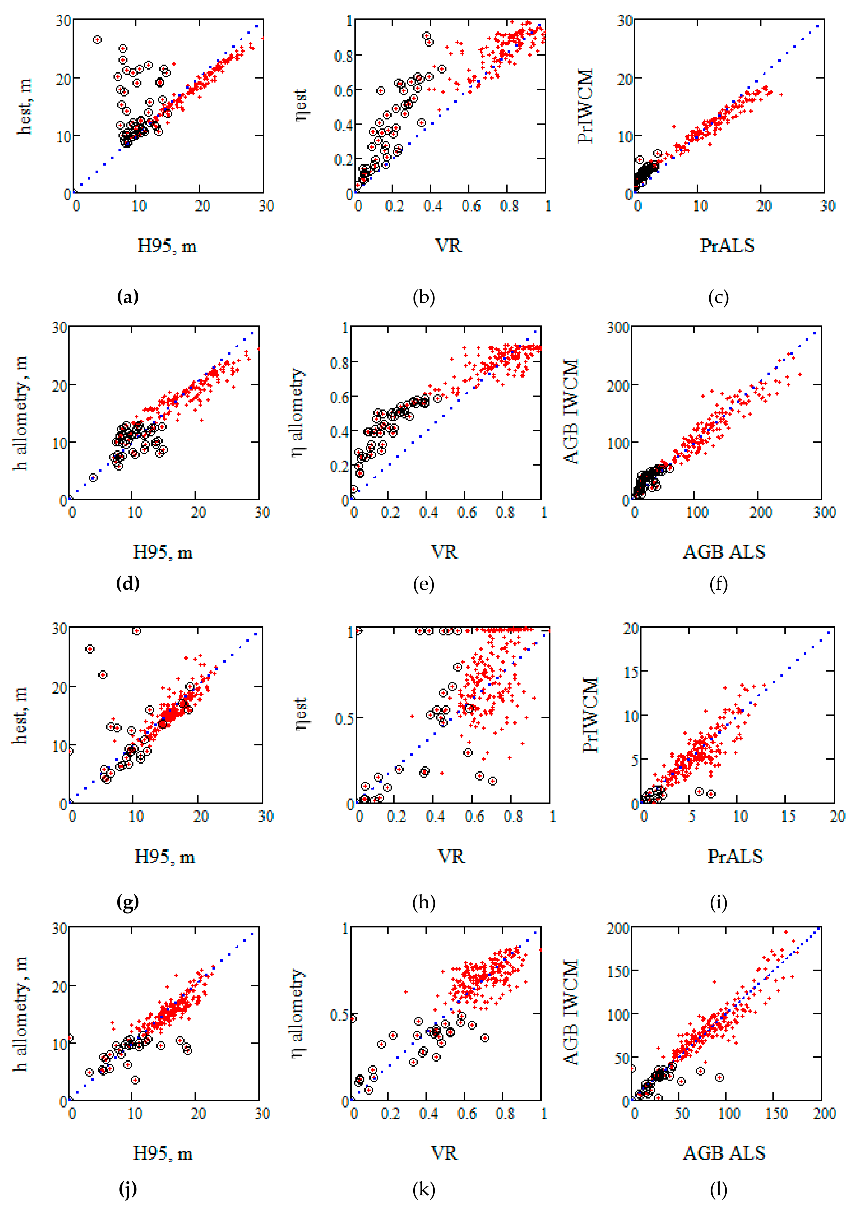
Stands in the large areas of Remningstorp and Krycklan are now analyzed regarding the structural properties height, area-fill and stem volume. Results are presented in Figure 4, where the solutions of Equation (4) are denoted hest and ηest, and in Table 4. Due to the sensitivity to ground conditions, stands with small phase heights, i.e., below 5 m, are marked by a black o in Figure 4. It also illustrates two products of height and density, PrIWCM = (hest – 1/α) ηest and PrALS = (H95 – 1/α) VR. These products take into account the changes of α, which might change due to summer/winter conditions. From Figure 4 we see a close relationship between these two products. In addition to expressions based on Equation (4), height and area-fill based on the allometry, h(Vestst) and η(Vestst), are illustrated. Vestst is the estimated stem volume according to the first step solution of IWCM. We also include estimates of AGB, and PrALS versus PrIWCM which agree well, independent of the phase height.
Many of the stands with deviations from the ALS observations possess a phase height <5 m. For this reason the stands were divided into two groups, those with a phase height below 5 m and those above. When Ph is less than the penetration depth 1/α the ground influence is the largest and AGB is small. These stands are not very homogeneous and at the same time the coherence is high, but variable. This complicates the solution of Equation (4) which assumes that the coherence is equal to γsys when the phase height is zero. γsys is based on an area in all inversion models and it cannot be determined for an individual stand. For the area-fill, the spread is larger and in this case the allometric expression Equation (2) seems to be the best alternative. We used the solutions of Equation (4) when the phase height was >5 m, and the allometric expressions h(Vestst) and η(Vestst) when the phase height was <5m in the case study with forest changes, with the estimates denoted h IWCM and η IWCM.
It should be noted from Figure 4 that the problem associated with hest and ηest for small phase heights is neither obvious in the estimation of the products introduced above nor AGB.
The results are summerized in Table 4.
5.3. Results from Case Study With Known Changes
The analysis of stands in Remningstorp and Krycklan resulted in general relationships between TanDEM-X and ALS data and also in new expressions for estimating height and density by means of IWCM. These results were applied to plots where management changes had taken place. There were 4 × 12 plots of 0.28 ha each at the test site Remningstorp, where the actions had occurred between 2010 and 2014, see [33]. The groups of stands represent pre-commercial thinning (PCT, lower vegetation removal, often with DBH <0.07 m), commercial thinning (T, commonly denoted only thinning, where about 30–35% of the basal-area is removed, but most often the suppressed trees are removed to gain the highest, remaining trees), and clear-cutting (CC, more or less all trees removed but sometimes seed trees are left, cf. Figure 1). The plots with no other changes than natural growth are denoted “untouched” (UT).
Four of the plots, that were clear-cut plots before 2014, had negative phase heights of around -0.16 m for three and -0.35 m for one. In the IWCM analysis these values were regarded as zero, and they can also be considered as a measure of the errors in the phase height estimation.
When investigating the data it was found that one clear-cut plot in 2011 had a low phase height but AGB >200 Mg/ha. This indicates that the clear cut took place between 2010 and 2011. This plot was therefore omitted. Three clear-cut plots had largely varying H95 with a standard deviation above 5 m. These plots were assumed to be clear cuts, but with seed trees left, and they are specially marked in the following. We also noticed rather low phase heights for the clear-cut plots after the change and of the pre-commercially thinned plots both before and after change. In the following the allometric relations were used to determine the height and area-fill for phase heights below 5 m, and otherwise expressions from Equation (4) were used.
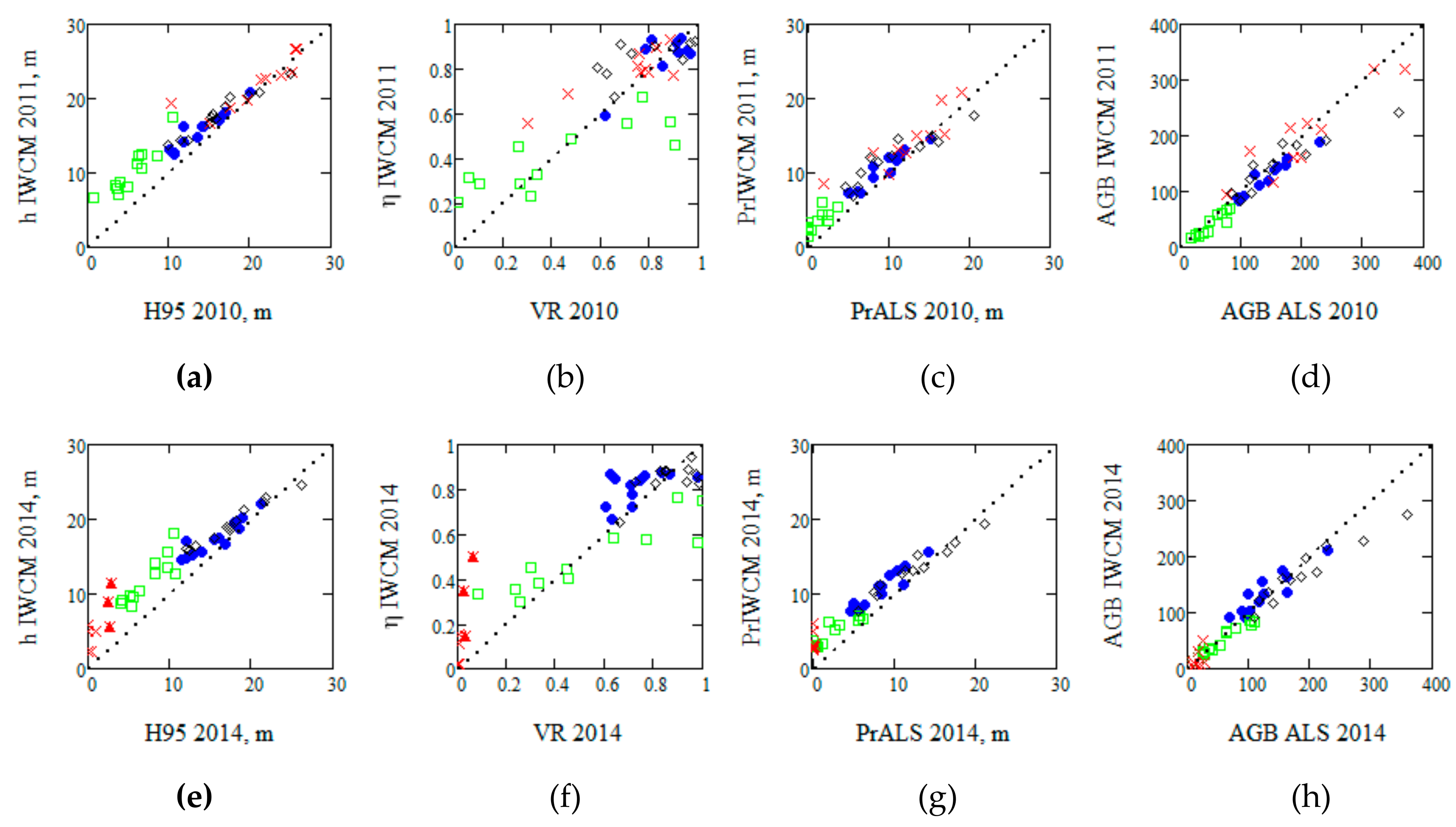
In Figure 5 and Table 5 and Table 6 the estimates of height and horizontal vegetation density from 2010/2011 and 2014 are compared with estimates coming from either TanDEM-X/IWCM or ALS. A high correlation was noticed between the height estimate h IWCM and H95 but this correlation decreased for plots with low height such as the pre-commercially thinned plots and the clear cuts after change. These plots also showed an over-estimation of height and varying estimates of horizontal vegetation density, particularly when the vegetation ratio was high. This effect was partly expected from the general analysis of Equation (4). It is related to the different sensitivities of η IWCM and VR for low heights. TanDEM-X may penetrate through the vegetation and gaps more irregularly and ALS is using definitions with height cutoffs. In addition, the forest may be less homogeneous at low heights. Figure 5 illustrates PrIWCM versus PrALS and here some over-estimation for low PrALS can be noticed while AGB IWCM shows some under-estimation for large AGB ALS. This may be related to the fact that the IWCM-parameters (including α) were estimated from “large areas” and AGB ALS was also estimated based on “large area” properties.
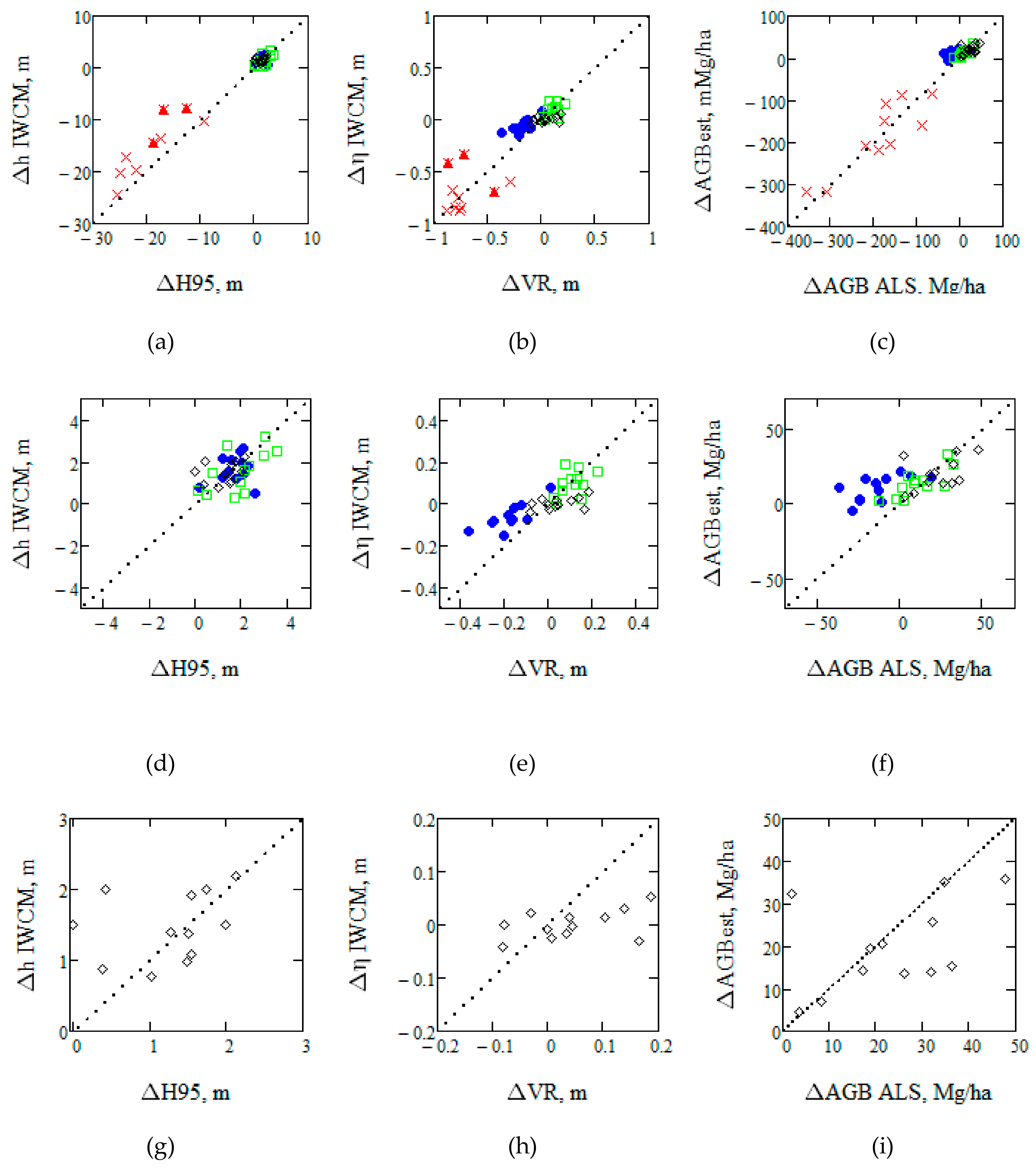
In Figure 6 estimates of the changes in height, density, and AGB were studied as determined by TanDEM-X/IWCM and ALS. In the upper row of Figure 6, the changes are well related. However, for the individual groups, the correlations are lower since the changes are close to the measurement accuracy. The middle row of Figure 6 is an enlarged part of the upper row. A clear relationship between area-fill and VR changes can be seen, as well as with AGB changes, but with a lower range of variation according to TanDEM-X/IWCM compared to ALS. For the untouched plots this is illustrated more in detail in the bottom row of Figure 6. The 12 untouched plots had a mean height growth of 2.7% and a mean AGB growth of 4.3% per year according to the TanDEM-X observations. Correspondingly, an H95 growth of 2.1% and an AGB growth of 4.2% per year were obtained from ALS. The latter results were corrected for the time between the ALS observations, 3.93 years, and between the TanDEM-X observations, 3.16 years. This is an approximate correction since the growth change is mainly related to the seasons. It should also be remarked that the untouched plots are a mixed group of plots with varying heights between 10 and 24 m, including plots to be thinned or even ready for clear cut, which means that AGB may vary quite a lot while the vegetation density is relatively constant. The results are summarized in Table 7.
5.4. TanDEM-X Versus ALS
ALS is considered the best remote sensing technique to study forest properties, but the airborne technique is expensive relative to satellite techniques per unit area. A question is to what extent ALS can be replaced by satellite bistatic observations e.g., TanDEM-X.
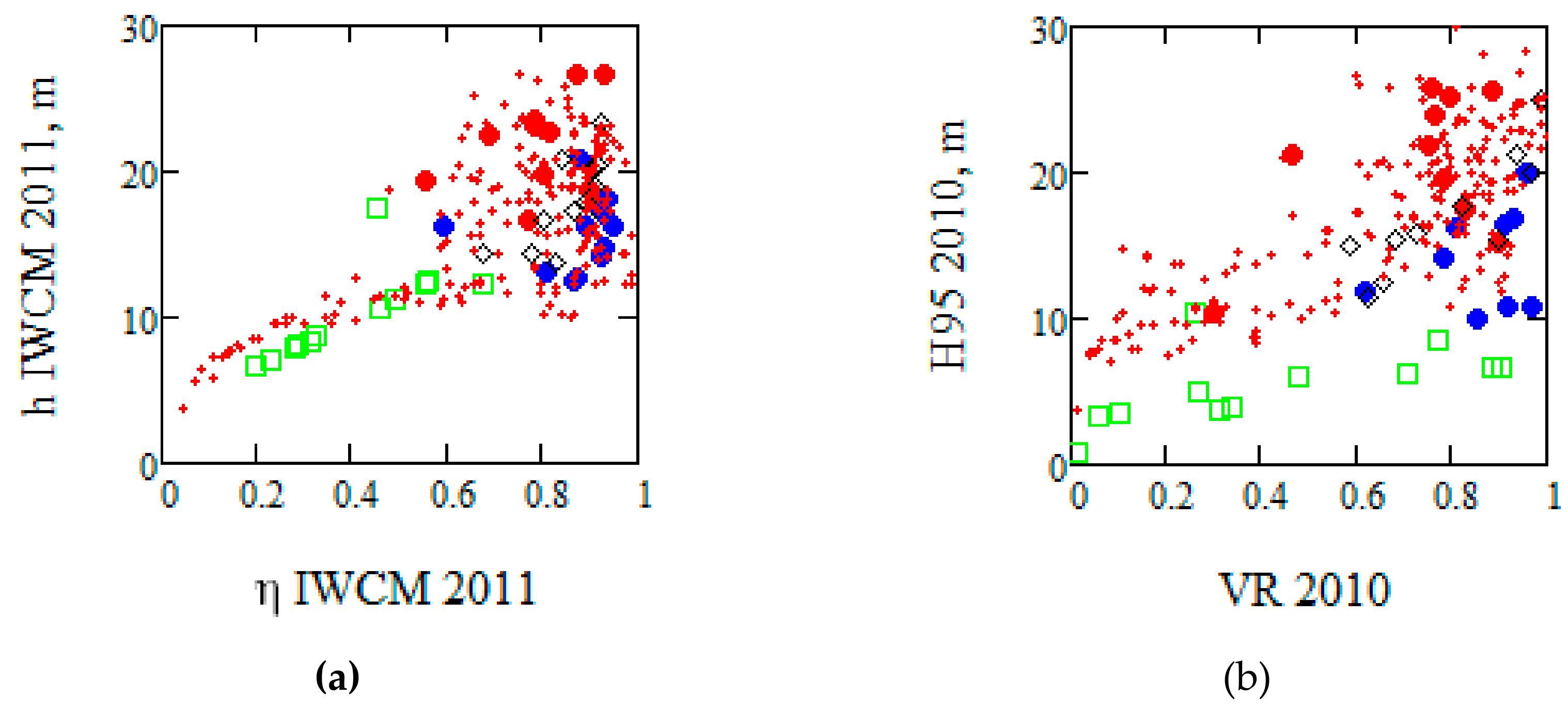
The large area in Remningstorp and Krycklan and the special stands with changes in Remningstorp gave two complementary pictures of observations by TanDEM-X/IWCM and ALS. The more than 200 stands at the study sites covered relatively large areas, represented different types of management and the stands were larger than 1 ha each. On the other hand, the 4 × 12 plots in Remningstorp (≈¼ ha) represented specific properties and known changes. The observations are illustrated in Figure 7.
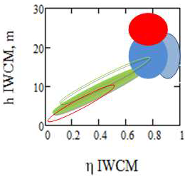
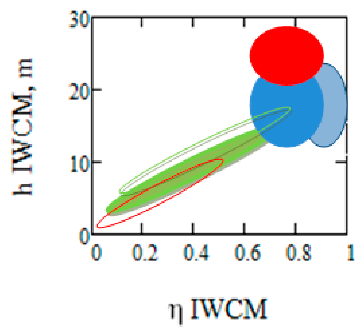
The untouched stands are not included in Figure 7 which illustrates different groups of stands with different properties. When investigating the changed forest plots, a difference can be seen in particular between the estimated heights of PCT by IWCM compared to ALS. PCT is supposed to take place at a mean height of 2–4 m which is in reasonable agreement with ALS. These stands had a phase height less than the approximate 5 m limit and they were then overestimated by IWCM. Stands in the range 0 < VR < 0.6 and 8 < H95 < 15 are probably stands that were pre-commercially thinned and followed by a height growth. Taking into account that height and density are estimated differently by TanDEM-X/IWCM and ALS, the findings can be represented in a schematic manner. In Figure 8 the different groups are illustrated as estimated by TanDEM-X/IWCM.
The different groups overlap to some extent, which is not surprising since the groups are not only defined by forest management principles but also by administrative aspects. The main overlap is between pre-commercially thinned stands and clear-cut stands which also include seed trees, for which the height and in particular the density were overestimated relative to ALS. However, the overlaps are of minor concern since affected stands (thinned or clear-cut) are already known.
Note that although a phase height/coherence diagram would show the properties of the different groups, such a diagram is dependent on HoA. This dependence is supposed to have been compensated by the IWCM-analysis.
6. Discussion
This paper is based on a comparison with ALS data acquired one or three years before the TanDEM-X acquisitions. The time difference might be an additional error source, nevertheless, the largest changes (clear cuts) could easily be identified and those stands and plots were omitted. In addition to the associated errors of the time discrepancy, the errors related to the ALS references were of the same order as the estimates based on TanDEM-X data. This means that the presented RMSEs are probably conservative.
We have observed a high correlation between ALS and TanDEM-X/IWCM data in spite of the differences in measurement techniques. The phase height has been shown to be proportional to the product of H95 and VegRatio for the studied acquisitions with an r2 in the order of 0.96 for Remningstorp and 0.85 for Krycklan. We have also found a strong correlation between the product of penetration height and area-fill for TanDEM-X/IWCM (hest − 1/α) ηest and for ALS (H95-1/α)VR with r2 in the order of 0.96 (Remningstorp) and 0.77 (Krycklan). It can be remarked that the high correlation between these products of penetration height and area-fill has also been verified for cold conditions (−10 °C) in Krycklan, 25 February 2012, studied in [12] which resulted in particularly low phase heights. The relationship is important since (H95-1/α)VR is closely related to phase height and only dependent on microwave properties through α which is dependent on frequency, meteorological conditions, and the vertical forest structure, and can often be neglected compared to H95.
For the 4 × 12 plots with specific changes, we find that the TanDEM-X/IWCM height is in good agreement with ALS H95 but with some overestimation for lower phase heights. Measurements of the horizontal vegetation density are more complex, in particular for stands with a low phase height, e.g., pre-commercially thinned (PCT) and clear-cut stands (CC) after clear cut. This is especially evident for PCT where VR varies over a very large range between stands (Figure 5) and also shows large variations of vegetation ratio within the individual stands with standard deviations up to 30%. H95 also has high standard deviation within the stands, up to 8.7 m for one stand, which indicates a large height variation. A special case is the clear cuts with seed trees, i.e., some high trees are left while the vegetation density is considerably decreased. The area-fill is rather overestimated compared to VR for stands with seed trees. Height is also overestimated relative to H95, which may also be related to the vegetation density dependence on H95 for clear cuts with seed trees left. These differences illustrate the different sensitivities for forest conditions of TanDEM-X and ALS, which are related to the measurement techniques, as well as the interpretations of the measurements.
On an individual plot basis, we see differences between the TanDEM-X/IWCM and ALS measurements, but, since we may be close to the accuracy limits, we also investigated the mean values of changes over groups of stands and the associated changes. In Table 7, the mean values are given for the change in estimated height, density, and AGB by TanDEM-X/IWCM and ALS between 2010/2011 and 2014. The range of AGB values associated with the groups of stands is also shown.
Figure 5 and Table 7 give two complementary pictures. From Figure 5 we see in particular a large range of vegetation ratio variation in the case of PCT. From Table 7 we see a discrepancy in the thinned plots regarding mean change of area-fill/VR and AGB. Assuming the thinning means a 30% reduction of the AGB, it favors the ALS information regarding AGB change since, with approximately the same growth variation with AGB as the untouched stands, the IWCM result may be interpreted as only a 15% reduction of AGB in the thinning. This indicates that the area-fill is not estimated in agreement with ALS in the case of thinned plots (according to Table 7) as well as PCT (according to Figure 5). PCT is characterized by a mean H95 of 5.4 m but a rather high variability in height while the mean vegetation ratio is 35%. The thinned stands, on the other hand, are characterized by a mean H95 of 14 m and small height variability but the mean vegetation ratio is 76%. Such conditions affect the gap frequency at the 41° incidence angle of TanDEM-X. The vegetation ratio determined by ALS with a relatively vertical measurement direction will cause a difference between the measurements. However, estimation of the top layer of the forest, height in the form of Lorey’s height, is not sensitive to the incidence angle in the same way and was estimated in good agreement with H95.
Two closely related papers to the present analysis are [10,33] investigating the same study sites as in this paper. The analyses in those papers were based on regression between field or ALS data and TanDEM-X phase height and coherence. Since local data are used for the investigation and the regression coefficients are optimized for each site it is expected that the estimated accuracy is high, about the same or higher than in this paper. Also, for the change analysis, which is based on regression, similar results are reported although the analyzed plots are not exactly the same. Karila et al. [40] investigated change detection by means of TanDEM-X digital surface models, of two TanDEM-X acquisitions from 2012 and 2014 and compared with ALS for a site in southern Finland. They used a regression technique for the InSAR digital surface model change and arrived at results indicating that the phase height change correlates more with vegetation density change than with height change. In the present paper the phase height was found to be equally sensitive to a relative variation of height and vegetation density but the difference in result seems related to how to compare a change in cover with a change in height.
Two other methods provide solutions of bistatic TanDEM-X data without the use of local data; solutions of height by means of Random Volume over Ground, RVoG, and of height and density by means of Two Level Model, TLM, (see Appendix A for description of models). Kugler et al. [30] used RVoG for analyzing a single polarization TanDEM-X VV acquisition in Krycklan and obtained RMSE = 1.58 m relative to H100 (for phase heights >4 m), while in this paper we obtained RMSE = 1.63 m relative to H95. Soja et al. [6] is based on TLM and reports (for phase heights >5 m) RMSE <10% for the TLM Δh relative to H50 and around 10% for canopy density for Remningstorp, while we obtained RMSE = 8% relative to H95 and 13% relative to vegetation ratio.
The difference between the models used to interpret bistatic TanDEM-X data, i.e., RVoG on one hand and IWCM and TLM on the other, is how the forest density is taken into account (this will also affect the volume decorrelation in IWCM). The sensitivity of the TanDEM-X phase height to ALS vegetation ratio, which is a proxy of scatterer density is illustrated in Figure 3. The effect on phase height is obvious since the phase height is zero for all phase components originating from vegetation gaps and ground scattering. The ground scattering is combined with scattering from the dense vegetation, mainly the top layer. Many papers have reported this sensitivity to forest density at X-band e.g., Garestier et al. [62] reported a 6 m height difference is measured between the different polarimetric phase centers over a sparse pine forest, probably due to the presence of holes in the canopy. Praks et al. [63] conclude that X-band inversion for tree height has a potential, at least in low-density forest ecosystems (e.g., boreal region). Garestier et al. [64] discussed the influence of density at X-band and the influence of gaps with effects on height estimation on PolInSAR and concluded that the performance of the vegetation analysis with the PolInSAR technique will be more density dependent at X-band. Solberg et al. [28] reported a relationship between X-band SRTM phase height measurements and stand density with r2 = 0.53. Praks et al. [65] reported varying height accuracy with varying density using RVoG and single polarization X-band.
A variation of forest density can be characterized either by a vertical or horizontal density variation in the models. IWCM assumes both a vertical and horizontal variation, in line with ALS observations, while RVoG assumes a vertical profile only. The profile normally used (Appendix A) assumes a constant density of scatterers with height and an exponential attenuation factor. The exponential attenuation is assumed to be the same for the dense parts of all stands in IWCM but varying with forest properties for RVoG. The latter then also represents horizontal variations of the scatterers. In order to study the varying vertical profiles, investigations have been done with multibaseline observations supported by information from lidar profile measurements, e.g., [66,67], by using PolInSAR and assuming various scattering profiles e.g., [68] or by using Legendre polynomials for the scattering profile and tomographic reconstruction e.g., [69] etc.
The analysis of vertical profile variations is mainly used for L- and P-band with the higher penetration into the vegetation layer compared to X-band, for which the main scatterers are leaves and twigs. Since interaction at X-band mainly takes place within the top canopy layer, forest can be characterized by a constant extinction, homogeneous, random volume [64].
ALS vegetation ratio is a commonly used measure of forest density and often preferred compared to a characterization using ALS vertical profiles. IWCM then offers a method to characterize horizontal density from single baseline, single polarization TanDEM-X observations. However, it should be noted that the solution of IWCM without the need for local training data is based on an allometric relationship between the area-fill and stem volume, a relationship that should be verified for the investigated area (cf. Appendix B). Nevertheless, IWCM may still be solved by means of training stands, cf. [4], without such assumption.
7. Conclusions
The goal of this paper was to estimate height, density, and stem volume/AGB from bistatic TanDEM-X data and a DTM, by means of IWCM solved without the need for local field data to train the model or for regression between properties. Instead, allometric relations were used to express height and density in stem volume.
Two study sites in Sweden, the hemi-boreal Remningstorp and the boreal Krycklan, were investigated using ALS and TanDEM-X with support of a DTM. The two sites are different in several aspects, hemi-boreal and boreal, managed differently by many owners or a single owner, different ranges of stem volume, different X-band backscatter characteristics, different topography etc. Large areas with more than 200 stands in Remningstorp and Krycklan were studied by means of TanDEM-X/IWCM in order to analyze structural properties such as AGB, height and vegetation density. The same allometric relations between Lorey’s height and stem volume as well as area-fill and stem volume were used for the two sites. The relationship for height was based on NFI data from Sweden. The allometric relationship for area-fill was verified by local field data in combination with TanDEM-X data. A simplified relationship between area-fill and vegetation ratio was determined as a constant.
A two-step solution of IWCM was applied. In the first step model parameters describing microwave properties of the forest were determined based on stands with a large range of stem volume. The stem volume of stands was also determined and then height and are-fill from the allometric relations. In a second step local estimates of height and density were determined. Due to sensitivity to ground conditions for low phase heights, a combination of the two results was suggested. However, we still see lower accuracy, in particular in the area-fill for low phase heights.
From the observations it was found that the phase height for summer conditions is approximately equal to the H95 times the vegetation density. This means that the phase height is equally sensitive to a relative variation of height and vegetation density. Estimates of AGB, height, and area-fill based on IWCM were compared with AGB, H95, and VR from ALS. AGB was determined with an RMSE of 17% for Remningstorp and Krycklan. With the local expressions for height and area-fill, height could be determined with an RMSE of 10% and 13% for all stands, and particularly for stands with phase heights above 5 m with an RMSE of 8% and 10%. Area-fill was found to be best estimated with allometry combined with estimated stem volume; the RMSE for Remningstorp and Krycklan was 21% and 15%, respectively, including all stands, and for stands with phase height above 5 m it was 13% in both cases.
By studying 4 × 12 plots with the three most common management changes (pre-commercial thinning, thinning and clear-cut) taking place between 2010 and 2014 plus untouched plots, individual plot properties could be studied. These different plots helped identify effects of small trees in dense plots (before pre-commercial thinning), large trees in plots with relatively high density (before thinning) and clear cuts left with seed-trees, and helped identify the effects on the interpretation of TanDEM-X bistatic observations. The area-fill, which is defined as the fraction of ground which is reached by microwaves attenuated by the vegetation layer, was found to be most affected by complex forest conditions related to high vegetation density or large height variations, effects believed to be caused by the high incidence angle and the variable forest conditions, but also due to the approximations associated with allometry for the area-fill.
Finally, the TanDEM-X/IWCM height and area-fill information was used for a schematic illustration of the different forest classes related to the need for management actions.
It is concluded that TanDEM-X can be quite useful for estimating boreal forest structural properties such as AGB, height, and vegetation density, and that the potential of bistatic SAR measurements of phase height (using a DTM as reference) in estimating these important properties of forest structure is that the phase height is closely related to height times vegetation density, and then to stem volume.
Author Contributions
J.I.H.A. proposed the paper and had the main responsibility for analysis of TanDEM-X data and for writing the major part of the paper, H.J.P. contributed with field and TanDEM-X data for the four areas with different change effects, analysis of ALS data and forestry aspects. All authors participated in detailed discussions about the paper.
Funding
This work was partly funded by the Swedish National Space Board Grants Dnr 164-16 and 300-16.
Acknowledgments
ESA and the BioSAR 2008 and BioSAR 2010 teams are gratefully acknowledged for funding and collecting the ALS and forest ground data covering the stands in Krycklan and Remningstorp. We are also grateful to Dr Maciej Soja for processing TanDEM-X scenes. DLR is acknowledged for TanDEM-X data distributed through proposal XTI_VEG0376 3D Forest Parameter Retrieval from TanDEM-X Interferometry (L.M.H. Ulander PI). Comments from the Academic Editor are acknowledged.
Conflicts of Interest
The authors declare no conflict of interest.
Appendix A. Model Expressions
The model equations are included for convenience. For details about IWCM, see [24,25]. The model assumes one part, 1−η, of the wave component is scattered directly from the ground, and one part, η, propagates through a vegetation cover and is scattered from the vegetation layer as well as an attenuated ground component
with and α is the attenuation in the vertical direction related to the extinction, κ, of the dense medium by α = 2κ/cosθI where θI is the incidence angle. In many papers e.g., [24,25] was assumed to be proportional to the stem volume V i.e., together with an associated demand on η to be ≤1. Later an allometric expression for η was introduced [5] and making a solution without local training data possible.
The ground to volume ratio is given by
The volume decorrelation is described by
where kz = 2π/HoA and HoA is the height of ambiguity.
The total coherence of the two incoherently added components from ground and vegetation is
where represent the temporal decorrelation plus system decorrelation γsys. For bistatic InSAR we have negligible temporal decorrelation and and we finally obtain
Finally, the phase height zest, and coherence, γ, are determined by
zest which is determined as a function of stem volume, V, is denoted Ph(V) in the text.
Appendix B. Area-Fill Expression
According to the observations, the phase heights of the studied acquisitions are (approximately) equal to the product of H95 and VegRatio, see Figure 3. This means for the model that Ph(V) should be equal to h(V) η(V)/κ, where κ represents the ratio between area-fill and VegRatio.
We may now assume η(ηm,ηsl,V) = ηm(1−e−ηslV), chose a set of parameters ηm, ηsl, derive the IWCM-parameters and determine Ph(V) = zest(α, m, γsys, ηm, ηsl HoA, V). κ(ηmηsl) is now determined as the root of
Vmax is the expected maximum stem volume for the area, for Remningstorp 500 m3/ha and for Krycklan 350 m3/ha.
We may also use the approximate relationship in Equation (3) to estimate optimal values of ηm, ηsl, and κ as those for which
has a minimum.
Results are given in Table A1 and illustrated in Figure A1. From Figure A1 we see that the model fit is not as good for Remningstorp as for Krycklan and also that a constant value of κ is not optimal in order to relate the area-fill to VegRatio, which will increase the RMSE of area-fill versus VR.

Table A1.
Optimal parameters for ηm and ηsl and results for ηm = 0.9 and ηsl = 0.01 with κ = 1.20.
| Site | ηm | ηsl | κ | RMSE V | RMSE h, All Stands | RMSE h, Ph > 5 | RMSE η, All Stands * | RMSE η, Ph > 5 * |
|---|---|---|---|---|---|---|---|---|
| Remningstorp | 0.915 | 0.01 | 1.201 | 16.56 | 10.05 | 7.27 | 26.40 | 16.75 |
| Remningstorp | 0.90 | 0.01 | 1.20 | 16.67 | 10.45 | 7.84 | 25.38 | 15.10 |
| Krycklan | 0.91 | 0.01 | 1.25 | 14.85 | 13.22 | 9.88 | 18.32 | 15.81 |
| Krycklan | 0.90 | 0.01 | 1.20 | 14.77 | 13.36 | 10.02 | 18.10 | 15.64 |
* based on allometry.
Figure A1.
Illustrating optimal results for Remningstorp (a,b), and Krycklan (c,d), between phase height and height∗density i.e. Hst versus H95st∗VegRatiost and Ph(V) versus h(V)η(ηm,ηsl,V)/κ(ηm, ηsl) in
(a,c); and VegRatio versus ALS stem volume versus (red dots), η(ηm,ηsl,V) versus V (black solid line), and η(ηm,ηsl,V)/κ(ηm, ηsl) versus V (black dashed line) in (b,d).


(The shift of VegRatio versus stem volume for zero stem volume is probably due to the fact that stem volume is only estimated in situ when DBH >0.04 m.)
References
- Shugart, H.H.; Saatchi, S.; Hall, F.G. Importance of structure and its measurement in quantifying function of forest ecosystems. J. Geophys. Res. Biogeosci. 2010, 115, 1–16. [Google Scholar] [CrossRef]
- WMO. The Global Observing System for Climate: Implementation Needs. Available online: https://bit.ly/2xAIaLe (accessed on 8 July 2019).
- Solberg, S.; Astrup, R.; Breidenbach, J.; Nilsen, B.; Weydahl, D. Monitoring spruce volume and biomass with InSAR data from TanDEM-X. Remote Sens. Environ. 2013, 139, 60–67. [Google Scholar] [CrossRef]
- Askne, J.I.H.; Fransson, J.E.S.; Santoro, M.; Soja, M.J.; Ulander, L.M.H. Model-based biomass estimation of a hemi-boreal forest from multitemporal TanDEM-X acquisitions. Remote Sens. 2013, 5, 5574–5597. [Google Scholar] [CrossRef]
- Askne, J.I.H.; Santoro, M. On the estimation of boreal forest biomass from TanDEM-X data without training samples. IEEE Geosci. Remote Sens. Lett. 2015, 12, 771–775. [Google Scholar] [CrossRef]
- Soja, M.J.; Persson, H.J.; Ulander, L.M.H. Estimation of forest biomass from two-level model inversion of single-pass InSAR data. IEEE Trans. Geosci. Remote Sens. 2015, 53, 5083–5099. [Google Scholar] [CrossRef]
- Karila, K.; Vastaranta, M.; Karjalainen, M.; Kaasalainen, S. Tandem-X interferometry in the prediction of forest inventory attributes in managed boreal forests. Remote Sens. Environ. 2015, 159, 259–268. [Google Scholar] [CrossRef]
- Toraño Caicoya, A.; Kugler, F.; Hajnsek, I.; Papathanassiou, K.P. Large-Scale Biomass Classification in Boreal Forests With TanDEM-X Data. IEEE Trans. Geosci. Remote Sens. 2016, 54, 5935–5951. [Google Scholar] [CrossRef]
- Soja, M.J.; Askne, J.I.H.; Ulander, L.M.H. Estimation of Boreal Forest Properties From TanDEM-X Data Using Inversion of the Interferometric Water Cloud Model. IEEE Geosci. Remote Sens. Lett. 2017, 14, 1–5. [Google Scholar] [CrossRef]
- Persson, H.J.; Fransson, J.E.S. Comparison between TanDEM-X-and ALS-based estimation of aboveground biomass and tree height in boreal forests. Scand. J. For. Res. 2017, 32, 306–319. [Google Scholar] [CrossRef]
- Persson, H.J.; Olsson, H.; Soja, M.J.; Ulander, L.M.H.; Fransson, J.E.S. Experiences from Large-Scale Forest Mapping of Sweden Using TanDEM-X Data. Remote Sens. 2017, 9, 1253. [Google Scholar] [CrossRef]
- Askne, J.I.H.; Soja, M.J.; Ulander, L.M.H. Biomass estimation in a boreal forest from TanDEM-X data, lidar DTM, and the interferometric water cloud model. Remote Sens. Environ. 2017, 196, 265–278. [Google Scholar] [CrossRef]
- Solberg, S.; Naesset, E.; Gobakken, T.; Bollandsås, O.-M. Forest biomass change estimated from height change in interferometric SAR height models. Carbon Balance Manag. 2014, 9, 1–12. [Google Scholar] [CrossRef] [PubMed] [Green Version]
- Solberg, S.; Gizachew, B.; Naesset, E.; Gobakken, T.; Bollandsås, O.M.; Mauya, E.W.; Olsson, H.; Malimbwi, R.; Zahabu, E. Monitoring forest carbon in a Tanzanian woodland using interferometric SAR: A novel methodology for REDD+. Carbon Balance Manag. 2015, 10, 1–14. [Google Scholar] [CrossRef] [PubMed]
- Treuhaft, R.; Goncalves, F.; dos Santos, J.R.; Keller, M.; Palace, M.; Madsen, S.N.; Sullivan, F.; Graça, P.M.L.A. Tropical-forest biomass estimation at X-band from the spaceborne TanDEM-X interferometer. Geosci. Remote Sens. Lett. IEEE 2015, 12, 239–243. [Google Scholar] [CrossRef]
- Treuhaft, R.; Lei, Y.; Goncalves, F.; Keller, M.; Santos, J.R.d.; Neumann, M.; Almeida, A. Tropical-Forest Structure and Biomass Dynamics from TanDEM-X Radar Interferometry. Forests 2017, 8, 277. [Google Scholar] [CrossRef]
- Solberg, S.; May, J.; Bogren, W.; Breidenbach, J.; Torp, T.; Gizachew, B. Interferometric SAR DEMs for Forest Change in Uganda 2000–2012. Remote Sens. 2018, 10, 228. [Google Scholar] [CrossRef]
- Hajnsek, I.; Kugler, F.; Lee, S.-K.; Papathanassiou, K.P. Tropical-Forest-Parameter Estimation by Means of Pol-InSAR: The INDREX-II Campaign. IEEE Trans. Geosci. Remote Sens. 2009, 47, 481–493. [Google Scholar] [CrossRef] [Green Version]
- Imhoff, M.L. Radar backscatter and biomass saturation: Ramifications for global biomass inventory. Geosci. Remote Sens. IEEE Trans. 1995, 33, 511–518. [Google Scholar] [CrossRef]
- Le Toan, T.; Beaudoin, A.; Riom, J.; Guyon, D. Relating forest biomass to SAR data. IEEE Trans. Geosci. Remote Sens. 1992, 30, 403–411. [Google Scholar] [CrossRef]
- Dobson, M.C.; Ulaby, F.T.; LeToan, T.; Beaudoin, A.; Kasischke, E.S.; Christensen, N. Dependence of radar backscatter on coniferous forest biomass. IEEE Trans. Geosci. Remote Sens. 1992, 30, 412–415. [Google Scholar] [CrossRef]
- Ulander, L.M.H.; Hagberg, J.O.; Askne, J. ERS-1 SAR Interferometry over Forested Terrain. In Proceedings of the Second ERS-1 Symposium, Hamburg, Germany, 11–14 October 1993; pp. 475–480. [Google Scholar]
- Hagberg, J.O.; Ulander, L.M.H.; Askne, J. Repeat-pass SAR interferometry over forested terrain. IEEE Trans. Geosci. Remote Sens. 1995, 33, 240–331. [Google Scholar] [CrossRef]
- Askne, J.; Dammert, P.; Ulander, L.M.H.; Smith, G. C-band repeat-pass interferometric SAR observations of the forest. IEEE Trans. Geosci. Remote Sens. 1997, 35, 25–35. [Google Scholar] [CrossRef]
- Santoro, M.; Askne, J.; Smith, G.; Fransson, J.E.S. Stem volume retrieval in boreal forests from ERS-1/2 interferometry. Remote Sens. Environ. 2002, 81, 19–35. [Google Scholar] [CrossRef]
- Santoro, M.; Askne, J.; Dammert, P. Tree Height Influence on ERS Interferometric Phase in Boreal Forest. IEEE Trans. Geosci. Remote Sens. 2005, 43, 207–217. [Google Scholar] [CrossRef]
- Kellndorfer, J.; Walker, W.; Pierce, L.; Dobson, C.; Fites, J.A.; Hunsaker, C.; Vona, J.; Clutter, M. Vegetation height estimation from shuttle radar topography mission and national elevation datasets. Remote Sens. Environ. 2004, 93, 339–358. [Google Scholar] [CrossRef]
- Solberg, S.; Astrup, R.; Bollandsås, O.M.; Næsset, E.; Weydahl, D.J. Deriving forest monitoring variables from X-band InSAR SRTM height. Can. J. Remote Sens. 2010, 36, 68–79. [Google Scholar] [CrossRef]
- Krieger, G.; Moreira, A.; Fiedler, H.; Hajnsek, I.; Werner, M.; Younis, M.; Zink, M. TanDEM-X: A satellite formation for high-resolution SAR interferometry. IEEE Trans. Geosci. Remote Sens. 2007, 45, 3317–3341. [Google Scholar] [CrossRef]
- Kugler, F.; Schulze, D.; Hajnsek, I.; Pretzsch, H.; Papathanassiou, K.P. TanDEM-X Pol-InSAR performance for forest height estimation. Geosci. Remote Sens. IEEE Trans. 2014, 52, 6404–6422. [Google Scholar] [CrossRef]
- Toraño Caicoya, A.; Kugler, F.; Pretzsch, H.; Papathanassiou, K. Forest vertical structure characterization using ground inventory data for the estimation of forest aboveground biomass. Can. J. For. Res. 2015, 46, 25–38. [Google Scholar] [CrossRef]
- Soja, M.J.; Persson, H.; Ulander, L.M.H. Estimation of forest height and canopy density from a single InSAR correlation coefficient. Geosci. Remote Sens. Lett. 2015, 12, 646–650. [Google Scholar] [CrossRef]
- Persson, H.J.; Soja, M.J.; Ulander, L.M.H.; Fransson, J.E.S. Detection of thinning and clear-cuts using TanDEM-X data. In Proceedings of the 2015 IEEE International Geoscience and Remote Sensing Symposium (IGARSS), Milan, Italy, 26–31 July 2015; pp. 2907–2910. [Google Scholar]
- Sadeghi, Y.; St-Onge, B.t.; Leblon, B.; Simard, M. Canopy height model (CHM) derived from a TanDEM-X InSAR DSM and an airborne Lidar DTM in boreal forest. IEEE J. Sel. Top. Appl. Earth Obs. Remote Sens. 2016, 9, 381–397. [Google Scholar] [CrossRef]
- Olesk, A.; Praks, J.; Antropov, O.; Zalite, K.; Arumäe, T.; Voormansik, K. Interferometric SAR Coherence Models for Characterization of Hemiboreal Forests using TanDEM-X Data. Remote Sens. 2016, 8, 700. [Google Scholar] [CrossRef]
- Soja, M.J.; Persson, H.J.; Ulander, L.M.H. Modeling and Detection of Deforestation and Forest Growth in Multitemporal TanDEM-X Data. IEEE J. Sel. Top. Appl. Earth Obs. Remote Sens. 2018, 11, 3548–3563. [Google Scholar] [CrossRef]
- Solberg, S.; Yousif, O.; Persson, H. Different sensitivity of X-band phase height to the vertical and horizontal dimensions of growing stock. In Proceedings of the ForestSAT, College Park, MD, USA, 1–5 October 2018. [Google Scholar]
- Naesset, E.; Bollandsås, O.M.; Gobakken, T.; Solberg, S.; McRoberts, R.E. The effects of field plot size on model-assisted estimation of aboveground biomass change using multitemporal interferometric SAR and airborne laser scanning data. Remote Sens. Environ. 2015, 168, 252–264. [Google Scholar] [CrossRef]
- Askne, J.I.H.; Persson, H.J.; Ulander, L.M.H. Biomass Growth from Multi-Temporal TanDEM-X Interferometric Synthetic Aperture Radar Observations of a Boreal Forest Site. Remote Sens. 2018, 10, 603. [Google Scholar] [CrossRef]
- Karila, K.; Yu, X.; Vastaranta, M.; Karjalainen, M.; Puttonen, E.; Hyyppä, J. TanDEM-X digital surface models in boreal forest above-ground biomass change detection. Isprs J. Photogramm. Remote Sens. 2018, 148, 174–183. [Google Scholar] [CrossRef]
- Schlund, M.; Davidson, M. Aboveground Forest Biomass Estimation Combining L-and P-Band SAR Acquisitions. Remote Sens. 2018, 10, 1151. [Google Scholar] [CrossRef]
- Ghasemi, N.; Tolpekin, V.; Stein, A. Assessment of forest above-ground biomass estimation from polinsar in the presence of temporal decorrelation. Remote Sens. 2018, 10, 815. [Google Scholar] [CrossRef]
- Zhang, H.; Wang, C.; Zhu, J.; Fu, H.; Xie, Q.; Shen, P. Forest above-ground biomass estimation using single-baseline polarization coherence tomography with P-band PolInSAR data. Forests 2018, 9, 163. [Google Scholar] [CrossRef]
- Solberg, S.; Hansen, E.H.; Gobakken, T.; Naessset, E.; Zahabu, E. Biomass and InSAR height relationship in a dense tropical forest. Remote Sens. Environ. 2017, 192, 166–175. [Google Scholar] [CrossRef]
- Wang, C.; Wang, L.; Fu, H.; Xie, Q.; Zhu, J. The impact of forest density on forest height inversion modeling from polarimetric InSAR data. Remote Sens. 2016, 8, 291. [Google Scholar] [CrossRef]
- Li, W.; Chen, E.; Li, Z.; Zhang, W.; Jiang, C. Assessing performance of tomo-sar and backscattering coefficient for hemi-boreal forest aboveground biomass estimation. J. Indian Soc. Remote Sens. 2016, 44, 41–48. [Google Scholar] [CrossRef]
- Kugler, F.; Lee, S.-K.; Hajnsek, I.; Papathanassiou, K.P. Forest height estimation by means of Pol-InSAR data inversion: The role of the vertical wavenumber. IEEE Trans. Geosci. Remote Sens. 2015, 53, 5294–5311. [Google Scholar] [CrossRef]
- Ulander, L.M.H.; Gustavsson, A.; Flood, B.; Murdin, D.; Dubois-Fernandez, P.; Depuis, X.; Sandberg, G.; Soja, M.J.; Eriksson, L.E.B.; Fransson, J.E.S.; et al. BIOSAR 2010 Technical Assistance for the Development of Airborne SAR and Geophysical Measurements during the BioSAR 2010 Experiment, Final Report. Available online: https://earth.esa.int/c/document_library/get_file?folderId=87248&name=DLFE-1322.pdf (accessed on 8 July 2019).
- Petersson, H. Biomassafunktioner för Trädfraktioner av Tall, Gran Och Björk i Sverige; in Swedish with English Summary; Department of Forest Resource Management, Swedish University of Agricultural Sciences: Umeå, Sweden, 1999. [Google Scholar]
- Næsset, E. Predicting forest stand characteristics with airborne scanning laser using a practical two-stage procedure and field data. Remote Sens. Environ. 2002, 80, 88–99. [Google Scholar] [CrossRef]
- Holmgren, J. Prediction of tree height, basal area and stem volume in forest stands using airborne laser scanning. Scand. J. For. Res. 2004, 19, 543–553. [Google Scholar] [CrossRef]
- Naesset, E. Airborne laser scanning as a method in operational forest inventory: Status of accuracy assessments accomplished in Scandinavia. Scand. J. For. Res. 2007, 22, 433–442. [Google Scholar] [CrossRef]
- Askne, J.; Dammert, P.; Fransson, J.; Israelsson, H.; Ulander, L.M.H. Retrieval of forest parameters using intensity and repeat-pass interferometric SAR information. Proc. Retr. Bio-Geophys. Parameters Sar Data Land Appl. 1995, 1, 119–129. [Google Scholar]
- Treuhaft, R.N.; Madsen, S.N.; Moghaddam, M.; van Zyl, J.J. Vegetation characteristics and underlying topography from interferometric data. Radio Sci. 1996, 31, 1449–1495. [Google Scholar] [CrossRef]
- Treuhaft, R.N.; Siqueira, P.R. The vertical structure of vegetated land surfaces from interferometric and polarimetric data. Radio Sci. 2000, 31, 1449–1495. [Google Scholar] [CrossRef]
- Treuhaft, R.N.; Law, B.E.; Asner, G.P. Forest attributes from radar interferometric structure and its fusion with optical remote sensing. Aibs Bull. 2004, 54, 561–571. [Google Scholar] [CrossRef]
- Cloude, S.R.; Papathanassiou, K.P. Polarimetric SAR interferometry. IEEE Trans. Geosci. Remote Sens. 1998, 36, 1151–1165. [Google Scholar] [CrossRef]
- Attema, E.P.W.; Ulaby, F.T. Vegetation modelled as a water cloud. Radio Sci. 1978, 13, 357–364. [Google Scholar] [CrossRef]
- Askne, J.; Santoro, M. Experiences in boreal forest stem volume estimation from multitemporal C-band InSAR. In Recent Interferometry Applications in Topography and Astronomy; Padron, I., Ed.; InTech Open Access Publisher: London, UK, 2012; pp. 169–194. [Google Scholar] [CrossRef]
- Li, X.; Strahler, A.H. Geometric-optical modeling of a conifer forest canopy. Geosci. Remote Sens. IEEE Trans. 1985, GE-23, 705–721. [Google Scholar] [CrossRef]
- Liu, J.; Woodcock, C.E.; Melloh, R.A.; Davis, R.E.; McKenzie, C.; Painter, T.H. Modeling the view angle dependence of gap fractions in forest canopies: Implications for mapping fractional snow cover using optical remote sensing. J. Hydrometeorol. 2008, 9, 1005–1019. [Google Scholar] [CrossRef]
- Garestier, F.; Dubois-Fernandez, P.; Dupuis, X.; Paillou, P.; Hajnsek, I. PolInSAR analysis of X-band data over vegetated and urban areas. IEEE Trans. Geosci. Remote Sens. 2006, 44, 356–364. [Google Scholar] [CrossRef]
- Praks, J.; Kugler, F.; Papathanassiou, K.P.; Hajnsek, I.; Hallikainen, M. Height Estimation of Boreal Forest: Interferometric Model-Based Inversion at L- and X-Band Versus HUTSCAT Profiling Scatterometer. IEEE Geosci. Remote Sens. Lett. 2007, 4, 466–470. [Google Scholar] [CrossRef]
- Garestier, F.; Dubois-Fernandez, P.C.; Papathanassiou, K.P. Pine Forest Height Inversion Using Single-Pass X-Band PolInSAR Data. IEEE Trans. Geosci. Remote Sens. 2008, 46, 59–68. [Google Scholar] [CrossRef]
- Praks, J.; Antropov, O.; Hallikainen, M.T. LIDAR-aided SAR interferometry studies in boreal forest: Scattering phase center and extinction coefficient at X-and L-band. Geosci. Remote Sens. IEEE Trans. 2012, 50, 3831–3843. [Google Scholar] [CrossRef]
- Treuhaft, R.N.; Chapman, B.D.; Dos Santos, J.R.; Goncalves, F.G.; Dutra, L.V.; Graca, P.M.L.A.; Drake, J.B. Vegetation profiles in tropical forests from multibaseline interferometric synthetic aperture radar, field, and lidar measurements. J. Geophys. Res. Atmos. 2009, 114, 1–16. [Google Scholar] [CrossRef]
- Brolly, M.; Simard, M.; Tang, H.; Dubayah, R.O.; Fisk, J.P. A Lidar-Radar Framework to Assess the Impact of Vertical Forest Structure on Interferometric Coherence. IEEE J. Sel. Top. Appl. Earth Obs. Remote Sens. 2016, 9, 5830–5841. [Google Scholar] [CrossRef] [Green Version]
- Garestier, F.; Le Toan, T. Forest modeling for height inversion using single-baseline InSAR/Pol-InSAR data. IEEE Trans. Geosci. Remote Sens. 2009, 48, 1528–1539. [Google Scholar] [CrossRef]
- Cloude, S.R. Polarization coherence tomography. Radio Sci. 2006, RS4017, 1–27. [Google Scholar] [CrossRef]
Figure 1.
Photographs of some plots in Remningstorp, (a) after pre-commercial thinning; (b) after thinning; (c) close to being cut; and (d) after clear-cut (with seed trees).
Figure 1.
Photographs of some plots in Remningstorp, (a) after pre-commercial thinning; (b) after thinning; (c) close to being cut; and (d) after clear-cut (with seed trees).

Figure 2.
Airborne Lidar Scanning (ALS) observations of H95, vegetation ratio versus stem volume in Remningstorp (a) and Krycklan (b). The solid lines represent allometric relations.
Figure 2.
Airborne Lidar Scanning (ALS) observations of H95, vegetation ratio versus stem volume in Remningstorp (a) and Krycklan (b). The solid lines represent allometric relations.

Figure 3.
Phase height versus (a) H95, (b) vegetation ratio, (c) stem volume, and (d) the product of H95 and VegRatio in Remningstorp and (e–h) in Krycklan.
Figure 3.
Phase height versus (a) H95, (b) vegetation ratio, (c) stem volume, and (d) the product of H95 and VegRatio in Remningstorp and (e–h) in Krycklan.

Figure 4.
Results for Remningstorp (upper two rows of figures, a–f) and for Krycklan (lower two rows of figures, g–l). (a and g) height versus H95, (b and h) area-fill versus VR, and (c and i) PrIWCM = (hest − 1/α) ηest versus PrALS = (H95 − 1/α) VR. The results are based on Equation (4) in (a–c) and (g–i) and from allometry, Equations (1) and (2), using IWCM estimated stem volume/AGB in (d–f) and (j–k). Stands with phase height <5 m are marked by black circles. AGB in Mg/ha.

Figure 5.
(a) Height h IWCM versus H95, (b) area-fill η versus VR, (c) PrIWCM = (hest − 1/α)ηest versus PrALS = (H95 − 1/α) VR, and (d) AGB in Mg/ha from IWCM versus AGB from ALS. (a–d) from 2011 and the corresponding (e–h) from 2014. Thinned plots: blue filled circle, pre-commercially thinned: green square; clear cut: red x; untouched: black diamond. Red triangles mark clear cuts with seed trees.

Figure 6.
Estimated changes from TanDEM-X/IWCM compared with changes estimated from ALS, (a) Δh IWCM versus ΔH95, (b) Δη IWCM versus VR, and (c) ΔAGB IWCM versus ΔAGB ALS. (d–f), and (g–i) are details of (a–c). The lower row illustrates specifically the untouched plots. Thinned plots: blue filled circle, pre-commercially thinned: green square; clear cut: red x; untouched: black diamond. Red triangles mark clear cuts with seed trees.

Figure 7.
Illustrating all stands investigated in 2010/2011 (red dots) together with the properties of the plots that have changed until 2014 color coded: (a) IWCM data, (b) ALS data. Thinned stands 2014: blue filled circle, pre-commercially thinned 2014: green square; clear cut 2014: red filled circle.

Figure 8.
Schematic diagram of different groups of stands in Remningstorp, to be pre-commercially thinned: green area, after being pre-commercially thinned: green outline; before thinning: light blue; after thinning: dark blue; to be clear cut: red, after clear cut: red outline.
Figure 8.
Schematic diagram of different groups of stands in Remningstorp, to be pre-commercially thinned: green area, after being pre-commercially thinned: green outline; before thinning: light blue; after thinning: dark blue; to be clear cut: red, after clear cut: red outline.

Table 1.
Data associated with TanDEM-X observations. HoA: height of ambiguity.
| Site | Date | HoA, m | Temperature °C | Precipitation, mm |
|---|---|---|---|---|
| Remningstorp | 4 June 2011 | 49 | 22 | 0 |
| Remningstorp | 2 August 2014 | 49 | 23 | 0 |
| Krycklan | 17 June 2011 | 52 | 14 | 0 |
Table 2.
Coefficient of determination, r2, between TanDEM-X phase height and forest properties.
| Site | H95 | VegRatio | Stem Volume | H95 * VegRatio |
|---|---|---|---|---|
| Remningstorp | 0.87 | 0.75 | 0.92 | 0.96 |
| Krycklan | 0.71 | 0.59 | 0.83 | 0.85 |
Table 3.
Interferometric Water Cloud Model (IWCM) estimated parameters, the backscatter from ground, σgr; the backscatter from a dense vegetation layer, σveg; the vertical attenuation factor through a dense vegetation layer, α; and the coherence for the ground layer, γsys.
Table 3.
Interferometric Water Cloud Model (IWCM) estimated parameters, the backscatter from ground, σgr; the backscatter from a dense vegetation layer, σveg; the vertical attenuation factor through a dense vegetation layer, α; and the coherence for the ground layer, γsys.
| Site | σgr | σveg | α m−1 | γsys |
|---|---|---|---|---|
| Remningstorp | 0.26 | 0.24 | 0.24 | 0.92 |
| Krycklan | 0.12 | 0.43 | 0.12 | 0.82 |
Table 4.
RMSE in % and r2 for the estimation of forest properties stem volume, height and area-fill as compared with ALS estimates of stem volume, H95 and VegRatio (VR).
Table 4.
RMSE in % and r2 for the estimation of forest properties stem volume, height and area-fill as compared with ALS estimates of stem volume, H95 and VegRatio (VR).
| Site | Stem Volume | h All Stands * | h Stands Ph > 5 | η All Stands ** | η Stands Ph > 5 ** |
|---|---|---|---|---|---|
| Remningstorp | 16.7%/0.92 | 10.5%/0.92 | 7.8%/0.95 | 21.2%/0.87 | 12.7%/0.16 |
| Krycklan | 17.1%/0.85 | 13.4%/0.72 | 10.0%/0.71 | 15.1%/0.65 | 13.0%/0.12 |
* h for all stands is estimated with allometry when the phase height (Ph) is <5 and with Equation (4) when Ph > 5 m. ** η is estimated with allometry.
Table 5.
r2 for all 48 plots.
| All Plots | h IWCM | η IWCM | AGB | PrIWCM/PrALS |
|---|---|---|---|---|
| 2010/2011 | 0.83 | 0.68 | 0.79 | 0.84 |
| 2014 | 0.92 | 0.84 | 0.93 | 0.94 |
Table 6.
r2 for h IWCM versus H95 and VR for each group of plots (for clear-cutting (CC) all stands/stands without seed trees). PCT: pre-commercial thinning; T: commercial thinning; UT: untouched.
Table 6.
r2 for h IWCM versus H95 and VR for each group of plots (for clear-cutting (CC) all stands/stands without seed trees). PCT: pre-commercial thinning; T: commercial thinning; UT: untouched.
| Groups of Plots | PCT | T | CC | UT |
|---|---|---|---|---|
| 2010/2011/H95 | 0.86 | 0.91 | 0.30/0.88 | 0.95 |
| 2014/H95 | 0.78 | 0.86 | 0.87/0.65 | 0.97 |
| 2010/2011/VR | 0.67 | 0.59 | 0.28/0.86 | 0.29 |
| 2014/VR | 0.83 | 0.26 | 0.52/0.82 | 0.48 |
Table 7.
Differences between 2014 and 2010/2011 of mean values over groups of plots.
| Groups of 12 Stands | AGB Range | Δh IWCM | ΔH95 | ΔArea-Fill | ΔVR | ΔAGB IWCM | ΔAGB ALS |
|---|---|---|---|---|---|---|---|
| PCT | 17−109 | 1.7 | 1.9 | 0.09 | 0.11 | 13.7 | 10.9 |
| T | 70−230 | 1.7 | 1.7 | −0.06 | −0.18 | 10.5 | −13.2 |
| CC | 0 – 369 | −15.4 | −17.9 | −0.59 | −0.64 | −169.5 | −170.1 |
| UT | 84−360 | 1.5 | 1.2 | 0 | 0.04 | 19.8 | 23.3 |
AGB in Mg/ha, h and H95 in m, area-fill and VR as fractions.
© 2019 by the authors. Licensee MDPI, Basel, Switzerland. This article is an open access article distributed under the terms and conditions of the Creative Commons Attribution (CC BY) license (http://creativecommons.org/licenses/by/4.0/).
Share and Cite
MDPI and ACS Style
Askne, J.I.H.; Persson, H.J.; Ulander, L.M.H. On the Sensitivity of TanDEM-X-Observations to Boreal Forest Structure. Remote Sens. 2019, 11, 1644. https://0-doi-org.brum.beds.ac.uk/10.3390/rs11141644
AMA Style
Askne JIH, Persson HJ, Ulander LMH. On the Sensitivity of TanDEM-X-Observations to Boreal Forest Structure. Remote Sensing. 2019; 11(14):1644. https://0-doi-org.brum.beds.ac.uk/10.3390/rs11141644
Chicago/Turabian StyleAskne, Jan I. H., Henrik J. Persson, and Lars M. H. Ulander. 2019. "On the Sensitivity of TanDEM-X-Observations to Boreal Forest Structure" Remote Sensing 11, no. 14: 1644. https://0-doi-org.brum.beds.ac.uk/10.3390/rs11141644
Note that from the first issue of 2016, this journal uses article numbers instead of page numbers. See further details here.