Underwater Image Restoration Based on a Parallel Convolutional Neural Network †


1
State Key Laboratory of Integrated Service Networks, Xidian University, Xi’an 710071, China
2
Collaborative Innovation Center of Information Sensing and Understanding at Xidian University, Xi’an 710071, China
3
Department of Electrical and Computer Engineering, McMaster University, Hamilton, ON L8S 4K1, Canada
*
Author to whom correspondence should be addressed.
†
This paper is an extended version of our paper published in the 10th Asian Conference on Machine Learning, Beijing, China, 14–16 November 2018.
Remote Sens. 2019, 11(13), 1591; https://0-doi-org.brum.beds.ac.uk/10.3390/rs11131591
Submission received: 16 May 2019
/
Revised: 26 June 2019
/
Accepted: 27 June 2019
/
Published: 4 July 2019
(This article belongs to the Special Issue Remote Sensing Image Restoration and Reconstruction)
Abstract
:Restoring degraded underwater images is a challenging ill-posed problem. The existing prior-based approaches have limited performance in many situations due to the reliance on handcrafted features. In this paper, we propose an effective convolutional neural network (CNN) for underwater image restoration. The proposed network consists of two paralleled branches: a transmission estimation network (T-network) and a global ambient light estimation network (A-network); in particular, the T-network employs cross-layer connection and multi-scale estimation to prevent halo artifacts and to preserve edge features. The estimates produced by these two branches are leveraged to restore the clear image according to the underwater optical imaging model. Moreover, we develop a new underwater image synthesizing method for building the training datasets, which can simulate images captured in various underwater environments. Experimental results based on synthetic and real images demonstrate that our restored underwater images exhibit more natural color correction and better visibility improvement against several state-of-the-art methods.
1. Introduction
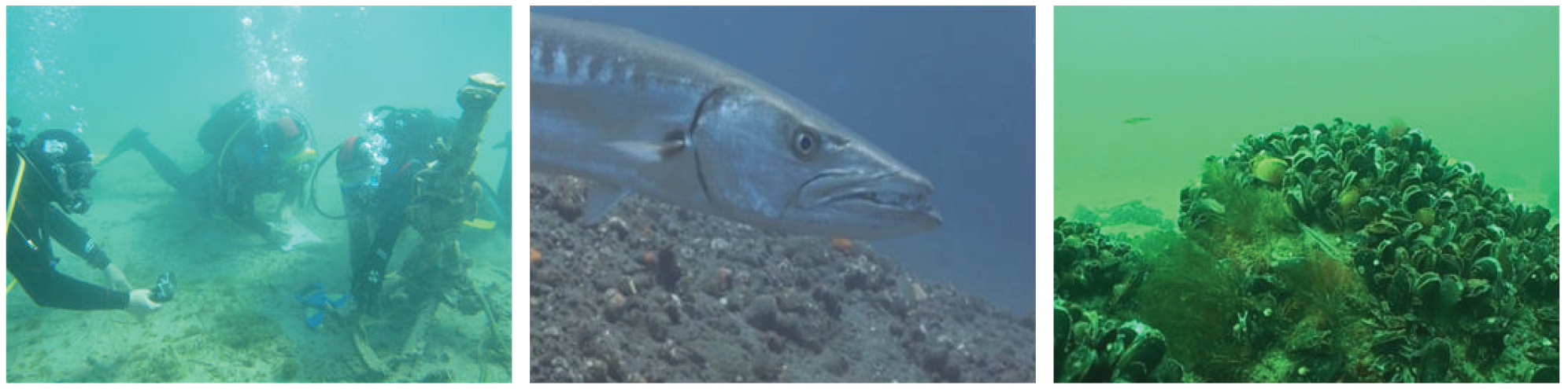
Underwater imaging has found important applications in diverse research areas such as marine biology and archaeology [1,2], underwater surveying and mapping [3], and underwater target detection [4,5]. However, captured underwater images are generally degraded by scattering and absorption. Scattering means a change of direction of light after collision with suspended particles in water, which causes the blurring and low contrast of images. Absorption means light absorbed by suspended particles which depends on the wavelength of each light beam [6]. Because the light with shorter wavelength (i.e., green and blue light) travels longer in water, the underwater images generally have predominantly green-blue hue. Contrast loss and color deviation are the main consequences of underwater degradation processes(e.g., Figure 1), which may cause difficulties for further processing, and it is of considerable interest to remove such distortions.
The goal of underwater image processing is to enhance visibility and rectify the color deviation. In general, the underwater image processing techniques can be divided into two categories, namely, underwater image enhancement and restoration [7,8]. The underwater image enhancement methods, such as histogram equalization [9], white balance [10], pixel stretching [11,12], retinex-based methods [13,14] and fusion-based methods [15,16,17], generally improve image visual effect by modifying image pixels without concerning the physical degradation mechanism of underwater images. These enhancement-based methods do not exploit physical imaging models and consequently they are often inadequate for restoring original scene features, especially color features [8].
On the other hand, underwater image restoration methods aim to recover clear images by exploiting the optical imaging model. The most important task for restoration is to estimate two key model parameters, i.e., transmission and ambient light, which are usually estimated either by prior-based approaches [6,18,19,20,21,22,23,24,25] or by learning-based approaches [26,27,28,29,30]. The prior-based approaches heavily depend on the reliability of certain prior information, such as dark channel prior [18,19,20,21], red channel prior [6], haze-line prior [25] and so on. However, priors generally have their respective limitations, and may not adapt to some conditions. Thus, a mismatch between the adopted prior and the target scene may incur significant estimation error, and consequently recover distorted results [23]. By contrast, the learning-based approaches aim to obtain more robust and accurate estimation by exploring the relations between the underwater images and the corresponding parameters in a data-driven manner, such as [26,27,28,29,30]. To this end, it is essential to have a suitable training dataset and an efficient neural network that can be trained to learn such relations. Unfortunately, the existing networks [26,27,28,29,30] are not capable of estimating the parameters accurately enough and the resulting restored images often suffer from various artifacts; it is also difficult to create a dataset capturing complex and varying underwater environments.
On the basis of the well-known model for underwater physical imaging, we propose a deep convolutional neural network (CNN) model with two parallel branches for underwater image restoration, accompanied by a training dataset in this paper. By exploring the inherent relations between the degraded underwater images and the associated blue channel transmission map as well as global ambient light in a data-driven manner, the proposed CNN can perform more accurate and robust parameter estimation; as a consequence, the restored images exhibit better visibility and more natural color compared to those produced by the state-of-the-art methods.
The contributions of this work are summarized as follows:
(1) We propose a new end-to-end underwater image restoration algorithm using a deep CNN model to improve the contrast and color cast of the recovered images. The whole network consists of two paralleled branches: a transmission estimation sub-network (T-network) and a global ambient light estimation sub-network (A-network), by which the transmission map and the ambient light can be estimated simultaneously. Since in our case no prior information is used to estimate the transmission and ambient light, it avoids the aforementioned mismatch issue commonly encountered in the prior-based methods and helps to improve the accuracy and universality of the estimation method.
(2) The proposed T-network is inspired by the U-shaped structure [31], but also has some additional features. In particular, it uses cross-layer connection and multi-scale estimation to preserve delicate spatial structures and edge features. Specifically, the cross-layer connection is used to compensate for the information loss, especially edge information while the multi-scale estimation helps incorporate local image details from different scales. These two special structures help to produce transmission maps with better edge features and prevent halo artifacts in restoration images. Indeed, good restoration results can be obtained based on the estimated transmission maps without any refinement.
(3) We design a new underwater image synthesizing method, which can produce synthetic images with different blue-green color cast and different degree of clarity based on the underwater image degradation model and the existing depth map datasets, effectively simulating images captured in different underwater environments. This method enables us to create a rich dataset of underwater images for network training.
The rest of this paper is organized as follows: Section 2 reviews the related work. Section 3 describes the proposed method in detail. Section 4 presents the experimental settings and results. Section 5 discusses the design idea underlying the proposed method. Lastly, Section 6 concludes this paper.
2. Related Work
Numerous methods have been proposed to enhance underwater degraded images in the past decade. Roughly speaking, these methods can be classified into two categories, namely, enhancement-based methods [10,11,12,13,14,15,16,17] and restoration-based methods [6,18,19,20,21,22,23,24,25,26,27,28,29,30]. Enhancement-based methods improve the image quality in a specific sense by using an image enhancement technique designed for that purpose. This type of methods can effectively improve the visual effect of the images. However, because the physical degradation principle is not considered and the relationship between degradation degree and scene depth is neglected, the enhancement results can not reflect the true color features of the scene correctly. On the contrary, the restoration-based methods use the constructed underwater imaging model to reverse the degradation process, for which it is necessary to estimate the unknown parameters: transmission and ambient light. If the model is properly constructed and the parameter estimation is accurate, the restored image will be close to the real scene. Depending on how parameter estimation is performed, they can be further divided into prior-based restoration methods and deep-learning-based restoration methods. In the following subsections, we mainly review the related works belonging to these two kinds of restoration methods.
2.1. Prior-Based Restoration Methods
Prior-based restoration methods extract image features through various priors and assumptions, and then estimate transmission and ambient light using these features to achieve image restoration.
In recent years, many methods have been proposed to estimate the transmission map of an underwater image using the Dark Channel Prior (DCP) [18], such as [19]. However, since the red channel rapidly loses intensity in underwater environments, the DCP tends to be violated. Therefore, various modifications of the DCP were proposed for underwater circumstances. For example, Drews et al. [20] proposed the Underwater Dark Channel Prior (UDCP), which ignores the red channel in the calculation of the dark channel; Galdran et al. [6] proposed the Red Channel Prior (RCP) which estimates the transmission by combining the inverse of the red channel and the DCP. Such modifications typically only lead to minor improvements in the accuracy of the estimation of the transmission map resulting due to the decrease in the reliability of the DCP prior. Given the observation that the red channel attenuates much faster than the green and blue ones, Carlevaris-Bianco et al. [21] proposed a new prior which estimates the depth of the scene with the aid of attenuation difference; see also Li et al. [22] for the application of this prior. Based on the same observation, Wang et al. [23] developed a new method, called maximum attenuation identification (MAI), to derive the depth map from degraded underwater images, and Li et al. [24] proposed to estimate medium transmission by reducing the information loss in a local block for red channel. However, due to the reliance on color information, these priors underestimate the transmission of objects with green or blue color. Berman et al. [25] suggested estimating transmission based on the Haze-Line assumption and estimating attenuation coefficient ratios based on the Gray-World assumption. However, this method may fail when the ambient light is significantly brighter than the scene because most pixels will point in the same direction and it is difficult to detect the haze lines.
Theoretically, as the depth in the scene increases, the transmission decreases to zero gradually and the ambient light makes more significant contribution. Thus, image pixels with maximum depth are often used to estimate ambient light as reference pixels. To select these reference pixels accurately, two general approaches have been proposed, which are based on color information and edge information, respectively. Chiang et al. [19] inferred ambient light from the pixel with the highest brightness value in an image. The authors in [6,22,23,24] chose pixels with the red channel intensity much lower than the blue and green ones as references. However, since reference pixels are selected according to color information, objects with same color may interfere in the selection process. Berman et al. [25] proposed to estimate ambient light according to the edge map associated with smooth non-texture areas. However, this method might not be suitable if the image contains a large object with smooth surface. Moreover, sometimes there is no ideal reference pixel in an image. For example, an image photographed from a downward angle may not contain pixels with deep depth.
Overall, the prior-based methods tend to make large estimation errors when the adopted priors are not valid. Lack of reliable priors for generic underwater images has become a significant hurdle impeding further progress in this direction.
2.2. Deep-Learning-Based Restoration Methods
Deep learning techniques have gained increasing popularity in image processing, and have been used for image transmission map estimation in particular [26,27,28]. Deep-learning-based methods rely on neural networks, trained by a large amount of data, to learn the relationship between an image and its associated transmission map. They can avoid, to a certain extent, the estimation errors incurred by invalid priors as seen in the prior-based methods. However, the neural networks that have been proposed so far are all for single-channel transmission estimation, with the implicit assumption that three color channels have the same transmission map. As such, they are only able to correct blurring and low contrast caused by scattering, but not color deviation induced by the discrepancies between the transmission maps of three channels commonly seen in underwater images.
Inspired by DehazeNet [26], Shin et al. [29] proposed an underwater restoration method based on deep learning, which estimates global ambient light and local transmission of underwater images using the same network, and then leverages the estimates to restore the clear image via the optical model. This method uses synthetic data for training. Specifically, the underwater image patches are simulated by adding different color deviation to the clear image patches, and the training label of each image patch is the corresponding transmission value or the ambient light value. Although this method achieves promising results, there are several aspects to be improved. In particular, due to the fact that local image patches are used as the training data (which lack global information) and that the discrepancies between the transmission maps of three channels are ignored in recovery, this method is often not able to estimate the parameters with sufficient accuracy and the restored images tend to suffer from color distortion and low clarify. A similar method was developed by Barbosa et al. [30], which estimates the transmission map and the ambient light respectively using a retrained DehazeNet and a prior proposed by Drews et al. [20].
It is well known that the performances of deep-learning-based methods depend critically on the quality of the training data. The training datasets used in [26,27,28] consist of haze images with no color deviation. The work by Shin et al. [29] uses a large number of training image patches with color deviation not specific to underwater environments, which are known to be mostly blue/green. For the purpose of transmission estimation, Barbosa et al. [30] rendered two 3D scenes and obtained a large set of images by positioning the camera in different locations, which are nevertheless still not sufficient to simulate diverse underwater environments. The lack of suitable training datasets has become a roadblock for the deep-learning-based approach to underwater image restoration.
3. Proposed Method
Aiming to improve the image contrast and color cast, an underwater image restoration approach based on a parallel CNN and the underwater optical model is proposed in this paper. We first briefly review the underwater optical imaging model, then present a detailed description of our proposed two-branch CNN framework and the loss functions used in the optimization. Next, we explain how to use the estimated transmission and global ambient light to restore the underwater images. Lastly, we propose a new underwater image synthesizing method that can be used to build the training datasets.
3.1. Underwater Optical Imaging Model
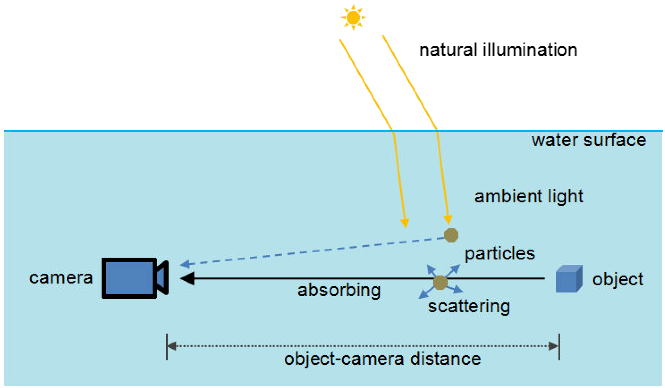
Figure 2 shows a schematic diagram of underwater optical imaging. In underwater photography, the light captured by the camera is mainly composed of two parts. One part of light is scene radiance which attenuates due to absorption of water and scattering of suspended particles. The other part of light is some ambient light reflected into the camera by suspended particles. Following the previous research [19], the simplified underwater optical imaging model can be described as:
where x denotes a pixel in the underwater image and c denotes the color channel, is the image captured by the camera, is the scene radiance, is global ambient light, and is the transmission map which represents the residual energy ratio of the scene radiance reaching the camera.
According to Schechner et al. [32], can be further expressed as:
where c denotes the color channel, is the object-camera distance, and is attenuation coefficient, which is a sum of the absorption coefficient and the scattering coefficient , i.e., .
Underwater image restoration aims to recover from . To this end, and need to be estimated first. Li et al. [24] found that the ratios of the total attenuation coefficients between different color channels in water can be expressed as:
where and are the red-blue and green-blue total attenuation coefficient ratios, respectively. is the wavelength of different color channels with , , equal to 620 nm, 540 nm, and 450 nm, respectively. Note that the transmission maps of the green and red channels, and , are determined by the blue channel transmission map, , as follows:
Therefore, the key issue of underwater image restoration is to estimate and accurately.
3.2. Proposed CNN Framework
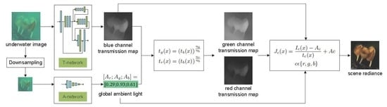
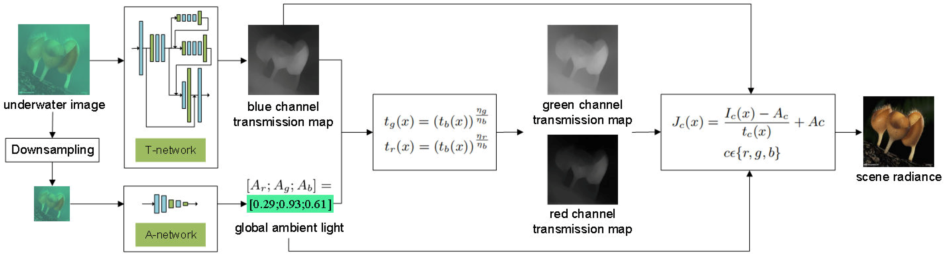
Our approach is to estimate the blue channel transmission and ambient light using two CNN subnetworks, respectively, and then leverage them to restore the clear images. The architecture of our approach is shown in Figure 3. Specifically, the T-network is used to estimate blue channel transmission map of the underwater image, and the A-network is used to estimate global ambient light. The transmission maps of red channel and green channel are then computed using Equation (4). Finally, the clear image is restored by substituting the obtained parameters into the underwater optical imaging model. The details of the A-network and the T-network are introduced as follows:
A-network: As mentioned in Section 2, most of the conventional methods intend to select the pixels with infinite depth to estimate ambient light. However, the accuracy of this selection is often limited by camera angle and jeopardized by some anomalous pixels. To address these issues and improve the robustness of the estimation, we proposed a new global ambient light estimation method based on CNN by learning the mapping between underwater images and their corresponding ambient light.
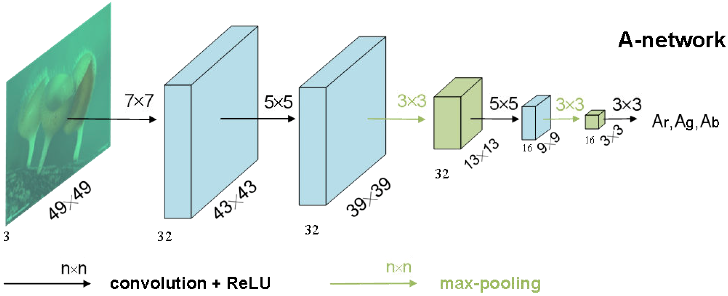
Considering the estimation of global ambient light is much easier than that of transmission, we design a light-weight CNN model called A-network to predict the global ambient light. The illustration of the A-network architecture is given in Figure 4.
The input of A-network is a down-sampled underwater image, and the corresponding output is the global ambient light, which is one pixel vector with three color channels, i.e., [; ; ]. Since the ambient light value is highly related to the global illumination features instead of the local image details, it is sensible to be estimated from a global perspective. In order to avoid the interference of the local details when extracting the global illumination features from the underwater image, the original image is down-sampled first before fed to A-network. Specifically, it is down-sampled to the size of to remove the most details but preserve the major global information as well. Meanwhile, by using an input down-sampled underwater image, the parameters of A-network can be greatly reduced, and the global image information can be learned more easily.
As shown in Figure 4, the A-network consists mainly of two operations: convolution and max-pooling. We use three convolutional layers to extract features and reduce the dimension of feature maps, and use two max-pooling layers to overcome local sensitivity and further reduce the resolution of feature maps. The last layer, which is also a convolutional layer, is used for nonlinear regression. We adopt a larger convolution kernel in the first layer, and then gradually reduce the size of the convolution kernels in the later layers with the decrease of the size of the feature maps. In such a way, a larger receptive field can be obtained and better global information which is related to the ambient light estimation can be learned. In addition, we add a ReLU layer after each convolutional layer to avoid the problems of slow convergence and local minima during the training phase.
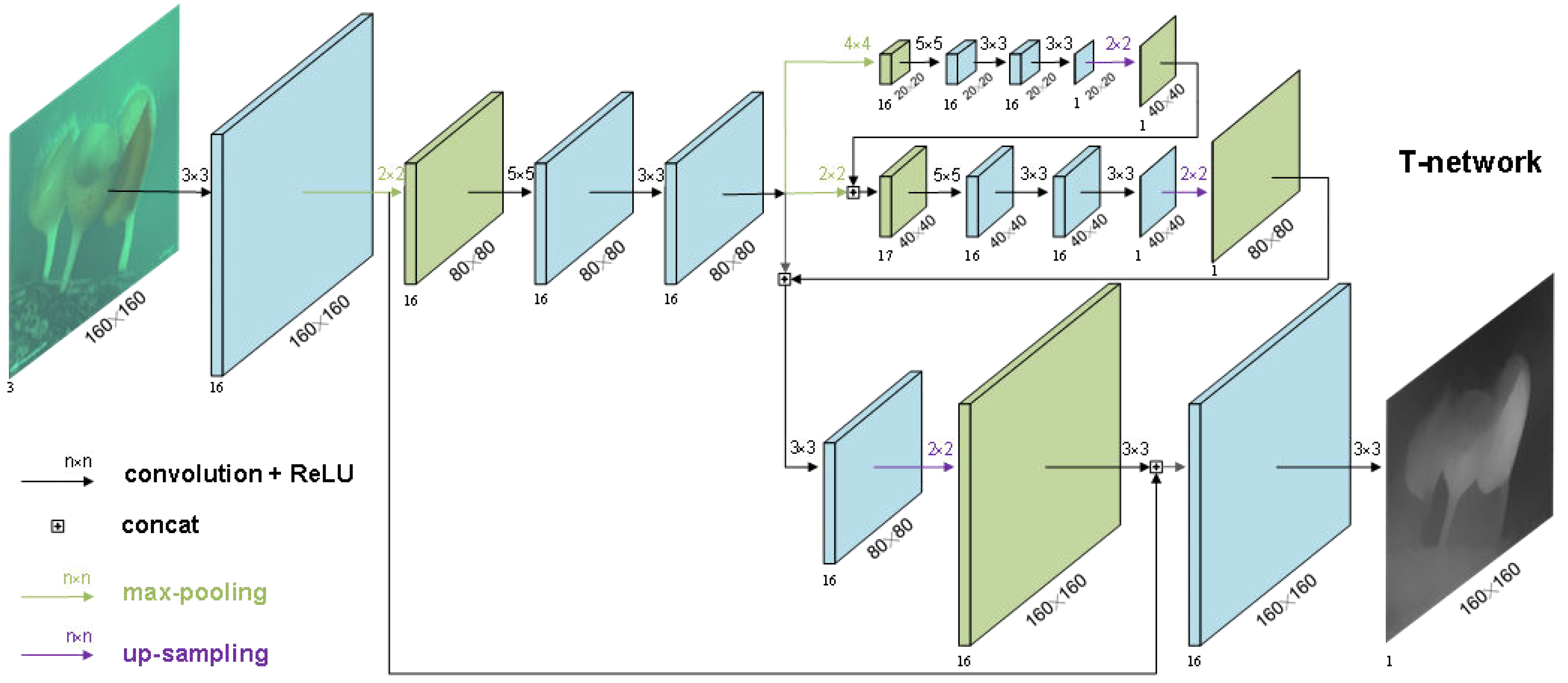
T-network: The existing CNN-based methods for transmission map estimation make the common assumption that the transmission maps of three color channels are the same. However, this assumption does not hold for underwater images. In general, blue light has the best transmission performance in water, and its transmission distribution is more uniform and wider. Based on the existing study of three-channel transmission relationship [24], the proposed method only estimates the blue channel transmission map, which is then leveraged to compute the other two transmission maps using the deterministic relationship among them. Such a two-stage estimation strategy simplifies the network structure and reduces the training complexity. In addition, the existing single channel transmission estimation network can be used for reference.
There are many research results in single channel transmission estimation methods. In [28], Zhao et al. proposed an end-to-end network, named Deep Fully Convolutional Regression Network (DFCRN), which has high accuracy in transmission estimation. The network uses a U-shaped network similar to encoding-decoding structure. In the encoding part, features are extracted. In the decoding part, features are preserved and re-extracted, and the size of output is ensured in this part. Under this U-shaped structure, this network can not only expand the receptive field, reduce the network parameters, but also ensure that the network has better nonlinear learning ability. However, this U-shaped network will lose some detail information, such as edges information, when reducing the size of the feature maps via the pooling layer in the encoding part. This makes the estimated transmission map unable to accurately reflect the edges shape, thus resulting in a halo phenomenon in the subsequent restored image. This phenomenon is common in the existing transmission estimation methods. Therefore, after estimating the transmission map, the edge-preserving filter is often used for refinement.
Building upon DFCRN, we design a new network (i.e., T-network) with enhanced edge preserving capability to estimate the blue channel transmission map, whose architecture is given in Figure 5. The proposed T-network is built by augmenting the basic U-shaped structure with some additional features, such as crosslayer connection and multi-scale estimation. The connection between the first convolutional layer and the penultimate convolutional layer is used to compensate for the information loss, especially edge information because the front layer still retains a lot of detail information, especially more abundant edges information. Moreover, we adopt a multi-level pyramid pooling as the second pooling layer, which helps to estimate the transmission in different scales. Inspired by Ren et al. [33], we fuse multi-scale transmission maps after the multi-level pyramid pooling, which helps to integrate features from different scales into the final result [34]. There is an up-sampling layer after the output of every scale. The output of small scale will be added to the next scale as a feature map. The multi-scale approach provides a convenient way to aggregate local image details associated with different resolutions [33], which helps to preserve edge features and prevent halo artifacts.
3.3. Loss Function
For regression tasks, most of the learning-based methods employ Euclidean loss, i.e., L2-norm loss, for network optimization. In this work, the L2-norm of the difference between the predicted and ground truth ambient light is used as the loss function to optimize the proposed A-network. Specifically, we define
where is L2-norm operation, is the output of the A-network, and is the corresponding ground truth ambient light with i denoting the color channel.
The transmission map estimated using only the L2-norm loss tends to be blurred and lacks high-frequency details, resulting in the loss of edge details. L1-norm loss is used to help to preserve the sharpness of edges and details. Thus, we optimize the T-network by minimizing a weighted combination of the pixel-wise L2-norm loss and L1-norm loss between the predicted transmission map and the corresponding ground truth. After experiments, the weight coefficient of L2-norm loss is 0.7, and the weight coefficient of L1-norm loss is 0.3. In addition, we adopt multi-scale estimation in our T-network, so the output of T-network has three different scales. The final loss function of our T-network can be expressed as the total loss on these three scales:
where is L2-norm operation, is L1-norm operation, N is the number of pixels in the input image, is the output of the T-network, and are small-scale outputs, is the corresponding ground truth transmission map, and are small-scale corresponding ground truth transmission map. is 16 times smaller than . is 64 times smaller than .
3.4. Image Restoration
Once the global ambient light and the blue channel transmission map are estimated by the A-network and the T-network, we can compute the green channel transmission map and the red channel transmission map using Equation (4). Finally, according to Equation (1), the scene radiance can be restored as follows:
where is the image captured by the camera, is the scene radiance, is global ambient light, and is the estimated transmission map with x denoting the pixel index and c denoting the color channel.
It is worth noting that many underwater image enhancement or restoration methods are patch-based, and consequently the resulting estimated transmission maps often suffer from serious block effect. To prevent halo artifacts in restoration images, guided image filtering [35] is often used to refine the transmission map by preserving the edge features. Different from those existing methods, the proposed method directly estimates whole transmission maps using our elaborately designed T-network, which can effectively prevent halos due to its good edge-preserving capability. Indeed, our method is able to produce more accurate estimated transmission maps with clear edges and consequently better restored images even without using guided filtering for post-refinement.
3.5. Synthesizing Underwater Dataset
The quality of the training data plays an important role in deep-learning-based methods. Training of CNN requires a large set of degraded underwater images and the corresponding clean images as well as the associated parameters (e.g., transmission map and global ambient light). It is very difficult, if not impossible, to obtain such a training dataset via experiments. Therefore, we choose to synthesize training images using the underwater optical model and the publicly available depth image datasets. Since underwater images generally have predominantly green-blue hue, we propose a method that can produce synthetic images with similar effects, effectively simulating images captured in various underwater environments. The detailed method is described as follows.
First, we collect clean images and the corresponding depth maps from the existing indoor and outdoor depth image datasets. It is preferable to have clean images with abundant colors and depth maps with clear edges. Next, we generate random blue channel attenuation coefficient , and global ambient light and then synthesize images using the physical model described in Section 3.1. The relationship between the transmission of three channels in [24] is used to reduce unknown parameters. Specifically, we first generate the blue channel attenuation coefficient, and calculate the blue channel transmission via Equation (2); the other two channels then can be calculated via Equation (4) and the underwater image can be generated via Equation (1). Because the red channel attenuates much faster in water, underwater images generally have predominantly green-blue hue. Thus, we assume that is smaller than and , and generate random , and . The dataset generated in this way can be used to train the network to have more accurate estimation of transmission and ambient light of underwater images with different green-blue hue color cast.
4. Experiments
In this section, we first further illustrate the proposed dataset synthesizing method, and then describe the experimental settings, and finally compare the proposed method with several state-of-the-art methods for single underwater image recovery, such as enhancement-based methods (Zhang et al. [12], Fu et al. [13]), prior-based methods (Drews et al. [20], Li et al. [24], Berman et al. [25]), and CNN-based methods (Shin et al. [29]), on the synthetic and real-world underwater images.
4.1. Dataset
Training datasets play an important role in deep-learning-based methods as they are used to learn the mapping between the data and the corresponding labels. Unfortunately, for the underwater image restoration problem, there is no sufficient amount of labelled data for network training, especially considering the diverse underwater environments. Therefore, we propose a method to generate synthetic images that can effectively simulate those captured in various underwater environments. The proposed method makes use of the existing depth image datasets, the underwater optical model and the prior that the red component of ambient light is smaller than blue and green components for under water images.
We choose Middlebury Stereo dataset [36,37] as the indoor depth dataset. In addition, we use clear outdoor images from the Internet and Liu et al. [38]’s depth map estimation model to generate the outdoor depth dataset. We crop images into smaller ones with size of pixels. Following the steps in Section 3.5, we use 477 clean images and corresponding depth maps to generate 13,780 underwater images and their corresponding transmission maps to train the T-network, and 20,670 underwater images and their corresponding ambient light to train the A-network. Note that the training images for the A-network are resized to pixels by nearest interpolation.
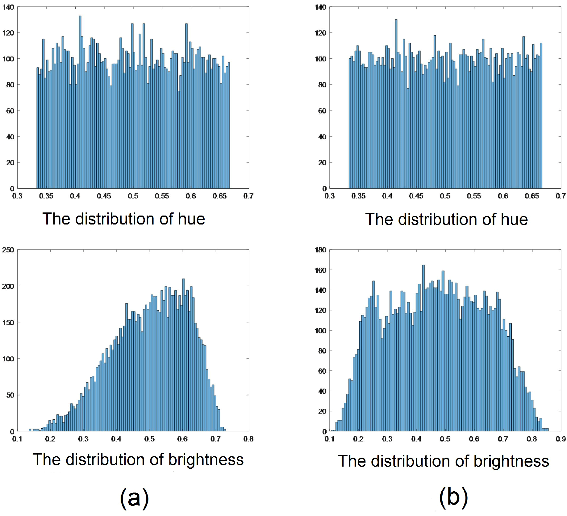
A good underwater dataset not only needs to cover a wide range of scenes in a uniform manner to avoid overfitting. In view of the fact that the diversity of underwater environments is reflected, to a significant extent, in ambient light, we carefully control the statistics of the hue and brightness of ambient light generated by our synthesizing method. First, consider using a uniform distribution defined over a certain range to generate ambient light. As shown in Figure 6a, ambient light generated in this way has an even distribution of green-blue hue color, but an uneven distribution of brightness. Thus, we modify the distribution by increasing the proportion of dark ambient light, the final distribution of is shown in Table 1 and the distribution of ambient light is shown in Figure 6b. It can be seen that our modification yields even distributions of hue and brightness.
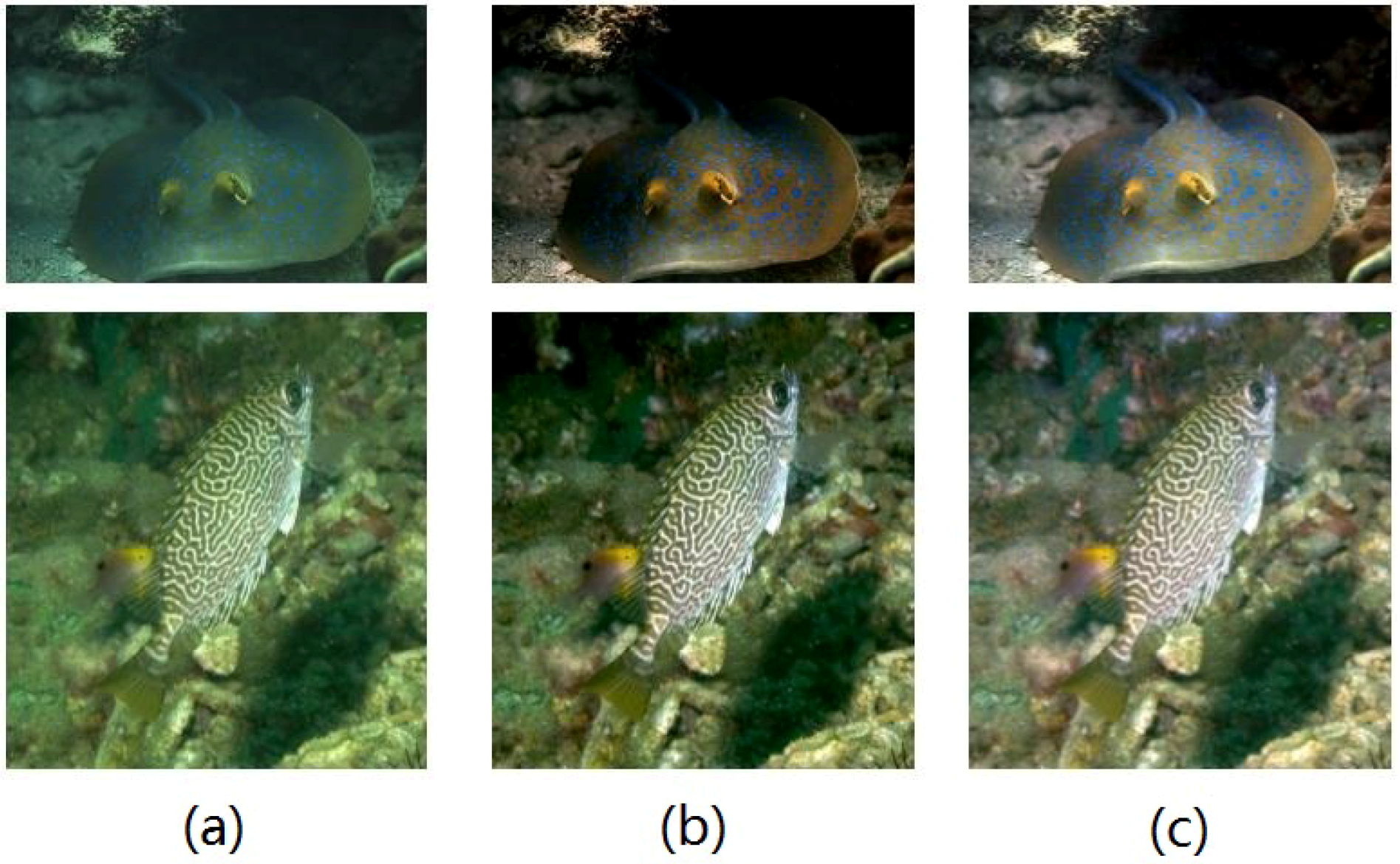
To demonstrate that datasets with evenly distributed hue and brightness improve the training performance, we compare the restoration results based on the datasets generated using the two aforementioned ambient light distributions. The comparison results are showed in Figure 7. It can be seen that the network trained with the dataset generated using the modified distribution performs better, especially on dark underwater images.
4.2. Experimental Settings
The back-propagation algorithm and the stochastic gradient descent (SGD) algorithm are used to train our models.
In our T-network, all the training samples are resized to . The batch size is set as 8. The initial learning rate is 0.001 and decreases by 10% after every 1 k iterations. The optimization is stopped at 20 k iterations. In addition, we set weight decay and momentum to 0.0001 and 0.9, respectively.
In our A-network, all the training samples are resized to . The batch size is set as 128. The initial learning rate is 0.001 and decreases by 10% after every 1 k iterations. The optimization is stopped at 20 k iterations. In addition, we set weight decay and momentum to 0.005 and 0.9, respectively.
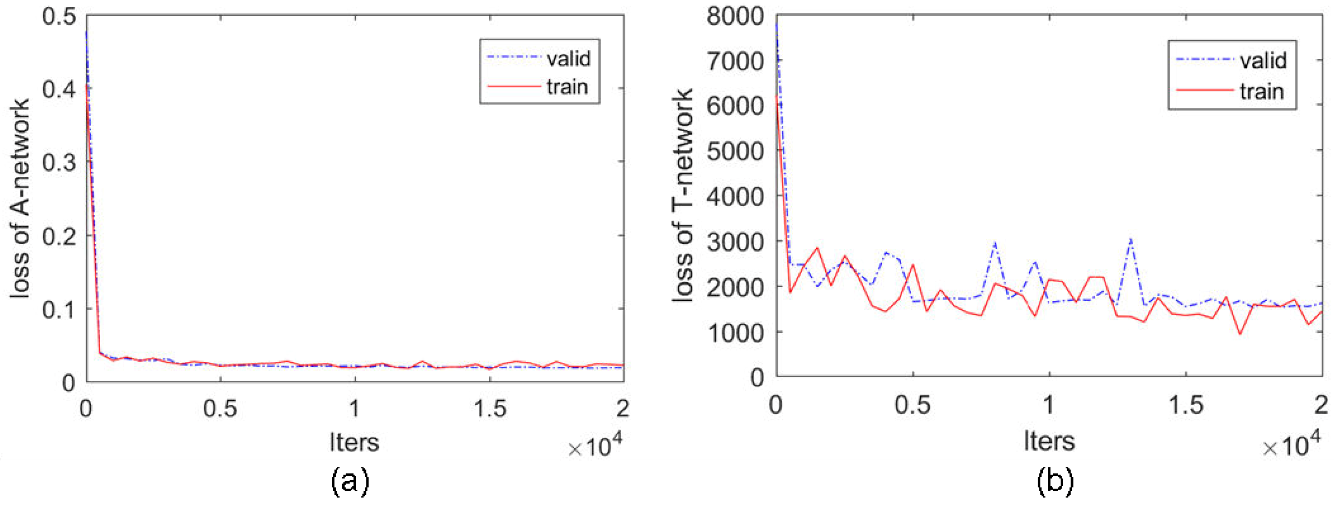
The training and validation loss of A-network and T-network over the training process are shown in Figure 8a,b, respectively. Note that training T-network requires more memory than A-network because the input/output size of T-network is much larger than that of A-network. Due to the memory limits of the device, a much smaller batch size is set in T-network training, which lead to a continuous fluctuation in the training loss curve of T-network, as depicted in Figure 8b. By considering that the validation loss curve of T-network converges after 15 k iterations, we stop the training process at 20 k iterations.
4.3. Comparisons on Synthetic Images
For evaluating performance, we construct a testing dataset of synthesized underwater images. We select 50 images and their depth maps from the NYU Depth dataset [39] and RESIDE dataset [40] (different from those that used for training) to synthesize 50 underwater images with different scenes, color deviation and contrast loss. Then, we evaluate the performance of the proposed method on the testing dataset and make comparisons with several state-of-the-art methods.
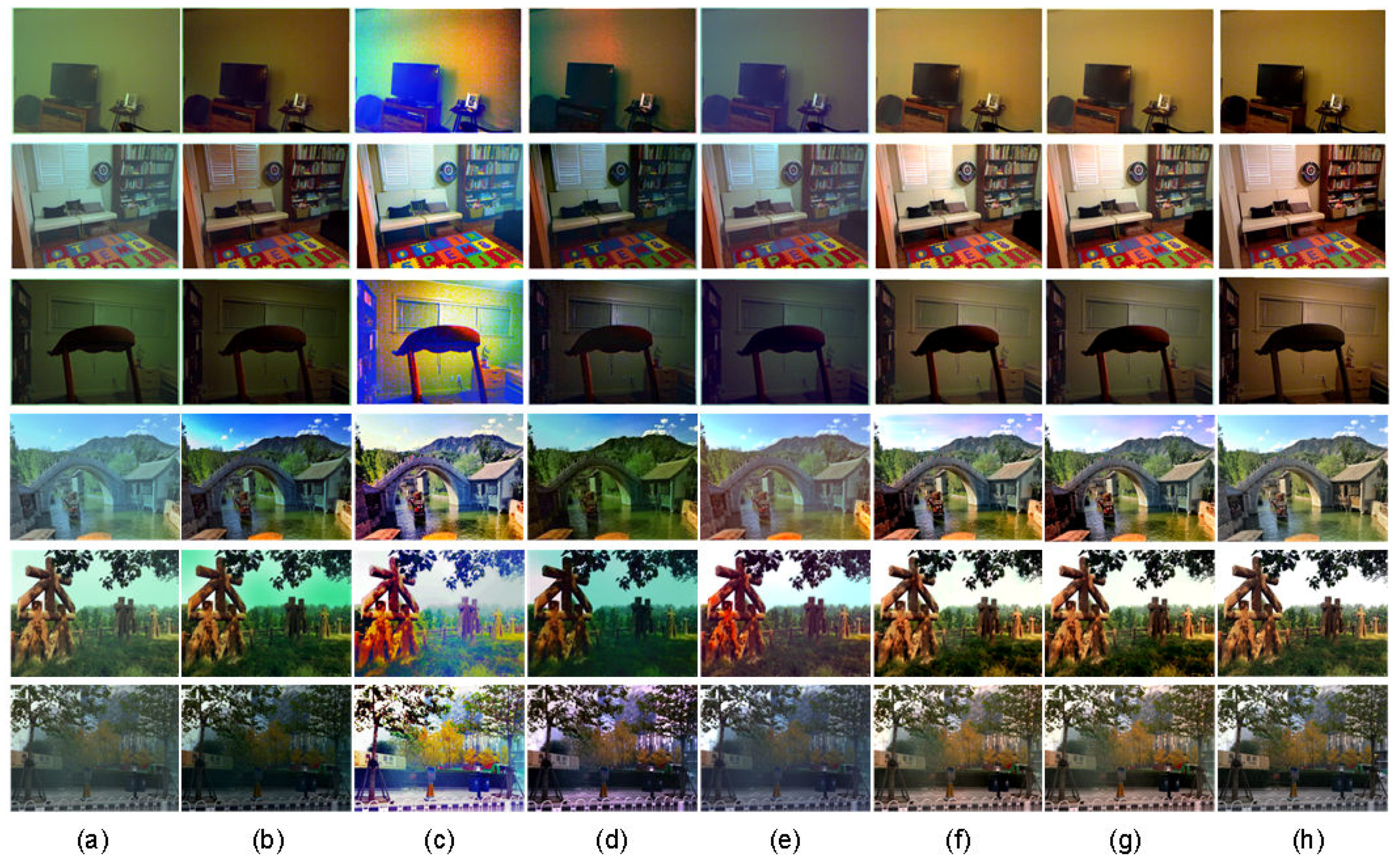
Figure 9 shows visual comparisons of different approaches on the testing dataset. As observed from Figure 9, Drews et al. [20] enhances image contrast to a certain extent, but fails to rectify color deviation sometimes. Li et al. [24] improves the visibility, but tends to produce over-enhanced results, as compared to the ground truth. Berman et al. [25] produces images with better clarity; nevertheless, the results still suffer from certain color deviation. Like our method, Shin et al. [29] also uses CNN to restore underwater images, but their results often exhibit low contrast, less details and color shift. By contrast, our method can not only improve the contrast of the degraded underwater images, but also correct the color deviation properly. Moreover, the images recovered using our method are visually closer to the ground truth clear images than those produced by the competing methods.
It should be noted that, since [20,24,29] are all patch-based, they have to use some edge-preserving filters, such as guided filters, to refine the estimated local transmission in order to suppress the block artifacts. In [25], guided filtering is also adopted to regularize the transmission map because a binary classification of the pixels often results in abrupt discontinuities in the transmission map.
Different from these state-of-the-art approaches, we elaborately design a CNN structure (namely, the T-network) with multi-scale estimation and cross-layer connection for transmission map estimation, which can well preserve edge features of the transmission map. Moreover, our method is designed for full-size input images, not just the local patches. Our network also benefits from the training dataset produced by the new synthesizing method, which can effectively simulate images captured in various underwater environments. As a consequence, our method can obtain more accurate estimation of transmission map and thereby restore images with clear edges. As shown in Figure 9f–h, the difference between our recovered images obtained with and without guided filtering is scarcely perceptible in most cases, and they both are very close to the ground truth. Therefore, guided filtering is inessential for our method as its functionalities have been implicitly realized by the proposed T-network.
Furthermore, we perform a quantitative comparison against the above-mentioned state-of-the-art restoration methods [20,24,25,29] using the Peak Signal-to-Noise Ratio (PSNR), Structural Similarity (SSIM) [41] and a color difference formula CIEDE2000 [42] as evaluation metrics. Specifically, a lager value of PSNR and SSIM, or a smaller value of CIEDE2000 indicates that the recovered image is closer to the corresponding ground truth in terms of statistical errors, image structure and color information, respectively. Table 2 summarizes the average values of SSIM, PSNR and CIEDE2000 for the restored images obtained by different methods. It can be seen that our method, without and with guided filtering (see Ours and Ours+GF in Table 2), outperforms the competing methods on all three metrics by a wide margin. It also shows that guided filtering is inessential for our method.
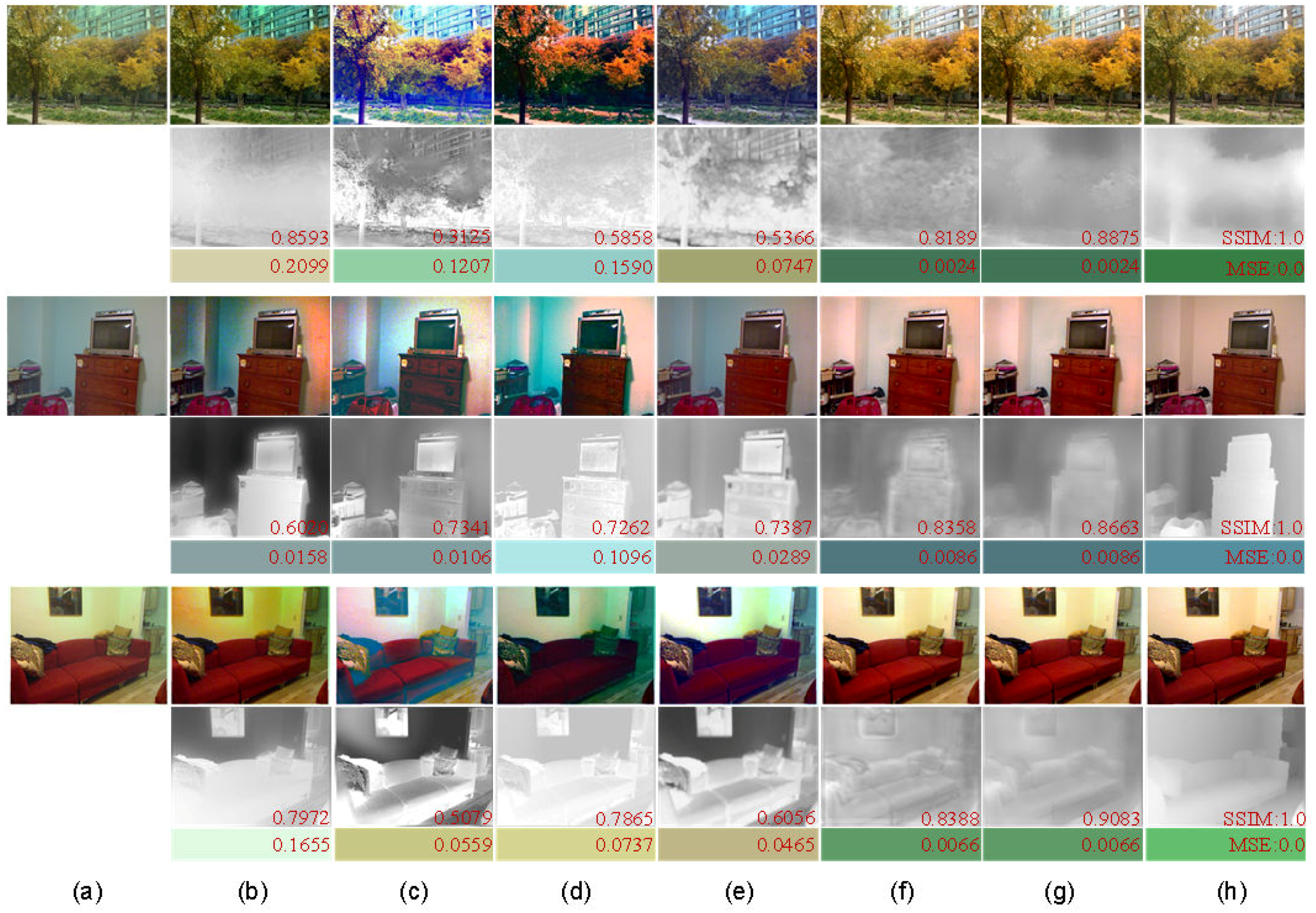
Finally, we compare the aforementioned restoration methods in terms of the accuracy of the estimated transmission light and global ambient light. Figure 10 illustrates the restored images and their correspongding estimated blue-channel transmission and ambient light by different methods. For the convenience of comparison, we visualize each ambient light as a colored bar. Note that [24,25] and ours first estimate single channel transmission, then compute the others; on the other hand, the authors in [20,29] do not take into account the difference between the three channels’ transmission. As such, in Figure 10, the comparison is made only regarding the blue channel transmission.
The accuracy of transmission and ambient light estimation determines the effect of image restoration. In Figure 10b–d, it can be observed that the results of the prior-based restoration methods [20,24,25] depend critically on the validity of priors. Specifically, Drews et al. [20], Li et al. [24] and Berman et al. [25] produce estimating error in some areas of transmission map due to the failure of their adopted priors based on color information. In addition, their estimated ambient light is not accurate, when there are no pixels with the same value as the actual ambient light in underwater scenes or they estimate ambient light at wrong location due to the failure of their adopted priors. Shin et al. [29] proposed a deep-learning-based method uses small local patches instead of full-size images as training samples; as such, it only exploits the local information but ignores the global structure. Owing to the limitation of the training data as well as the network architecture, this method produces relatively large estimation errors, especially regarding the ambient light, as illustrated in Figure 10e. Compared with the above-mentioned methods, our method produces more accurate estimation results. In particular, our estimated transmission maps reflect more correctly the depth relationship between objects, and our estimated ambient light has less color distortions, as shown in Figure 10f–g.
For further comparison, we compute the Mean Squared Error (MSE) of the estimated global ambient light and the SSIM of the estimated transmission maps produced by different methods. It can be seen from the quantitative results shown in Figure 10 that our method gives the most accurate estimation of both the transmission map and the ambient light.
4.4. Comparisons on Real-World Images
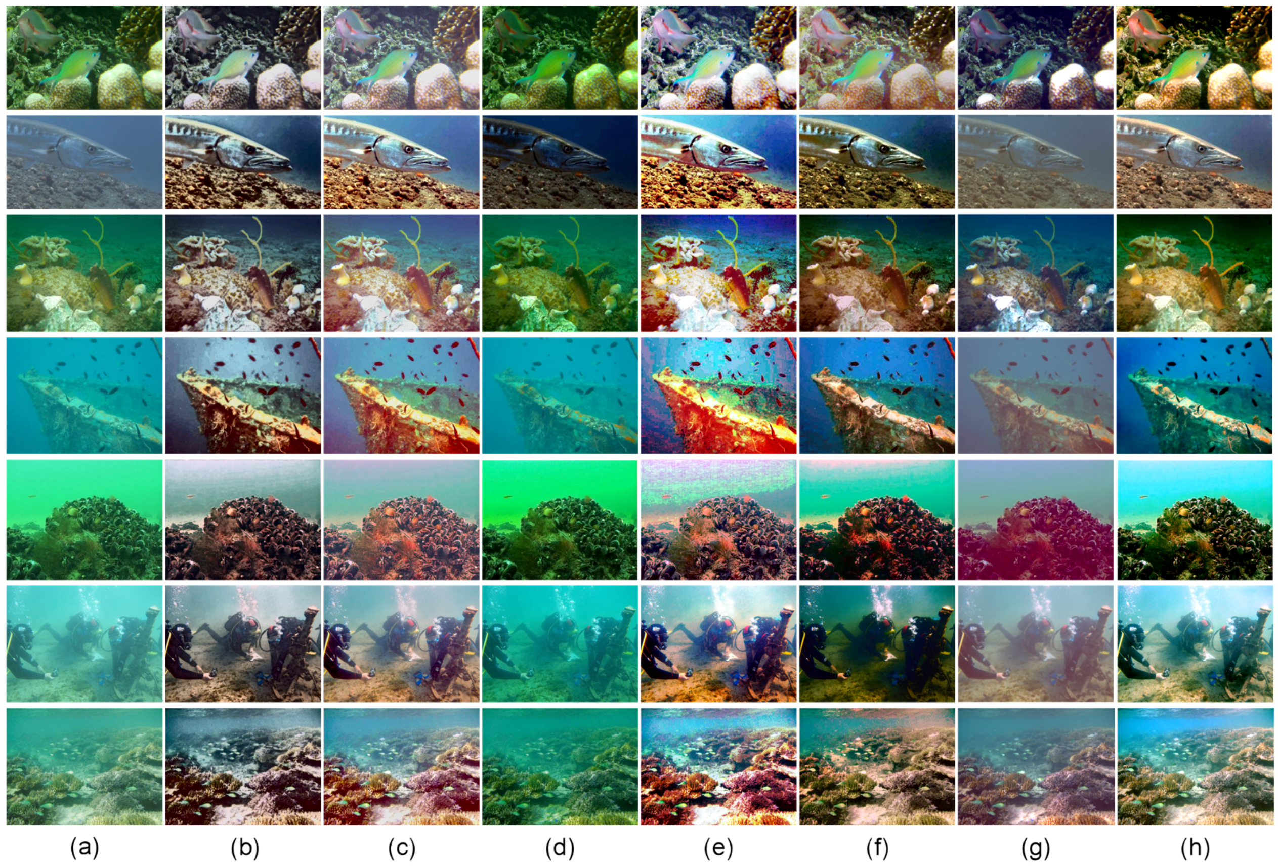
In this part, we conduct several comparisons on real-world underwater images in order to verify the effectiveness of the proposed method. We choose a number of challenging real-world images with diverse underwater scenes and color shift that are commonly used for qualitative comparisons. Figure 11 compares the recovered results of our method against several state-of-the-art methods on real-world images, including four restoration-based methods [20,24,25,29] mentioned in the previous subsection and two representative enhancement-based methods [12,13].
As shown in Figure 11b,c,e, the authors in [12,13,24] succeed in enhancing contrast of the recovered images and enriching the details, but they tend to over-enhance and produce reddish results. The authors in [20] can only increase the contrast of images, but fail to correct color deviation, as depicted in Figure 11d because it assumes that the attenuations of three color channels are the same, which is actually invalid in underwater environments. According to Figure 11f, the authors in [25] perform well on contrast enhancement and color correction, but it generates over-enhanced and over-saturated results when the ambient light is significantly brighter than the scene. It can be seen from Figure 11g that the results of [29] tend to have poor visibility with low contrast and hue distortion due to the inaccurately estimated transmission and ambient light. In contrast, our method produces images with natural color, enhanced contrast, and visually pleasing visibility, as illustrated in Figure 11h. Therefore, although the proposed network is trained using synthetic underwater images, it is capable of delivering more satisfactory restoration results on real-world degraded underwater images as compared to the state-of-the-art methods.
In addition, we use two non-reference image quality metrics to objectively evaluate the recovered underwater images obtained by different methods. One is the Blind/Referenceless Image Spatial Quality Evaluator (BRISQUE) [43], a metric for evaluating possible losses of naturalness in an image because of the presence of distortions. The range of BRISQUE scores is 0 to 100. The score closer to 0 represents the better quality. The other is the Underwater Color Image Quality Evaluation (UCIQE) [44], a metric to quantify the nonuniform color cast and low-contrast that characterize underwater images. A higher UCIQE score represents a better image quality. We use 50 real-world images with diverse underwater environments as a test dataset. Table 3 lists the average BRISQUE scores and UCIQE values for the different methods. As shown in Table 3, the proposed method outperforms the others.
5. Discussion
Among the existing underwater image restoration methods, the authors in [29] is most similar to ours. In particular, both methods use CNN to estimate unknown parameters, transmission and ambient light. In this section, we shall explain the reasons for the competitive advantage of our method.
5.1. Training Set
Both the method by Shin et al. [29] and the proposed one use synthetic underwater images for training. The difference is that in our method the whole underwater images are generated by using the existing depth datasets and the relationship between the transmission maps of three color channels is considered, whereas the work by Shin et al. [29] generates a large number of image blocks with the same depth and ignores the differences in the transmission maps of the three channels. In addition, the underwater image dataset generated by Shin et al. [29] contains a wide range of color cast not specific to underwater images. In contrast, we take into account the fact that the color cast of most underwater images is blue or green and constrain the value of red channel ambient light to the minimum; we are able to generate images containing only a variety of blue-green color cast, yielding a more realistic simulation of underwater images.
Figure 12 shows synthetic samples that simulate images captured in different underwater environments. It can be seen that different ambient light yields different blue-green color deviation, and a larger blue channel attenuation coefficient results in greater contrast loss.
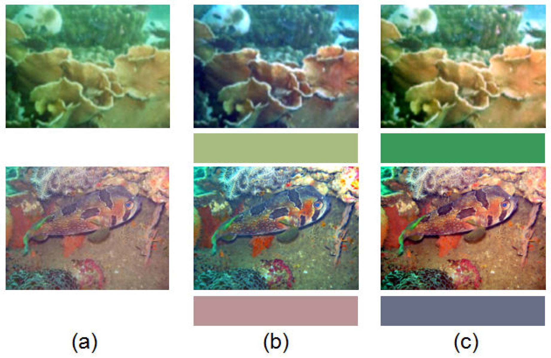
5.2. Ambient Light Estimation
The work by Shin et al. [29] uses the same network structure based on DehazeNet to estimate the ambient light value channel-by-channel. In contrast, we estimate the values of the ambient light of three channels at the same time using the proposed A-network, which reduces the number of parameters. Moreover, underwater images can be considered as a combination of clear images and ambient light images. The proportion of ambient light is reflected in the color cast of underwater images, and is related to depth. Considering that the depth information is helpful for ambient light estimation, we adopt the lower resolution underwater images generated by the depth maps via the underwater optical model as the training samples of the A-network. Since the image details are not important for estimating global ambient light, we reduce the size of A-network training images to improve the training speed. In the work by Shin et al. [29], small local patches (with the same transmission in each patch) are used as the training samples. Due to a lack of global depth information in the training dataset, the estimated ambient light produced by network in [29] is prone to the influence of the overall hue of the image, and the estimation error tends to be large when there is a significant difference between the overall hue of the image and the ambient light (e.g., considering underwater images with minor color deviation and small ambient light contribution, such as those taken from a close range).
Figure 13 compares the ambient light estimation results by [29] and ours. In theory, the hue of ambient light can be inferred from an area in the image with infinite depth. Due to inadequate learning of global depth information, the estimation results of [29] are affected by the color of close-range objects. In contrast, our method can avoid this issue and perform better in terms of color deviation correction.
5.3. Transmission Map Estimation
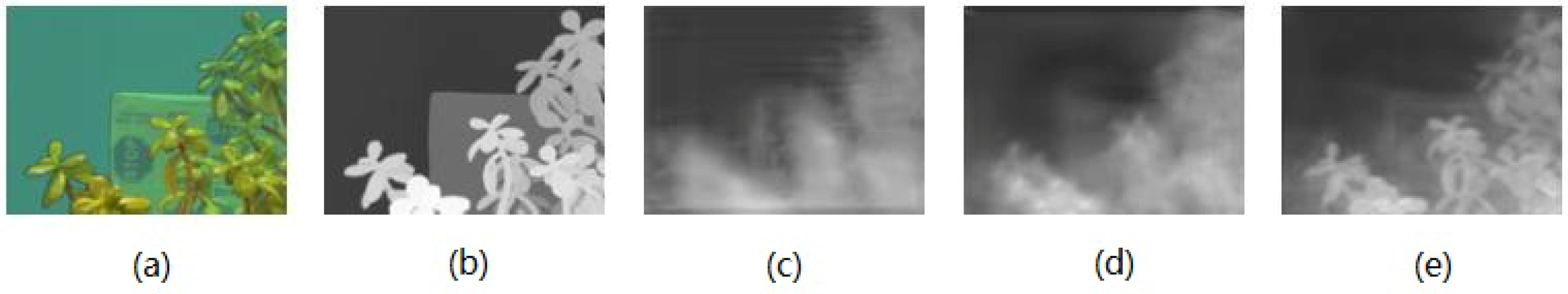
In the work by Shin et al. [29], a large number of small local patches (with the constant transmission map) are used to train the network for transmission map estimation. Because only local information is considered, the estimation results tend to be influenced by color information. In contrast, our network is trained using full-size images, thus acquires the ability to preserve global spatial structures. Moreover, the restoration result will likely suffer from halo artifacts when the depth boundary is not accurately captured in the transmission map. As Ref. [29] is patch-based, the estimated transmission map needs to be refined by guided filtering to prevent serious halo artifacts. However, this is not needed for our method due to the use of cross-layer connection and multi-scale estimation in the proposed T-network. To demonstrate that cross-layer connection and multi-scale estimation are essential for the edge-preserving ability of our T-network, we train three different networks using the same dataset generated by our synthesizing method and compare their respective transmission estimation results in Figure 14. As shown in Figure 14c, the U-shaped structure alone (DFCRN [28]) cannot preserve edge features well. With multi-scale estimation incorporated into the U-shaped structure, the resulting estimation shows more details (Figure 14d). The result further improves when both multi-scale estimation and cross-layer connection are added to the U-shaped (which becomes our T-network)—see Figure 14e. This ablation study clearly shows importance of cross-layer connection and multi-scale estimation.
5.4. Limitations
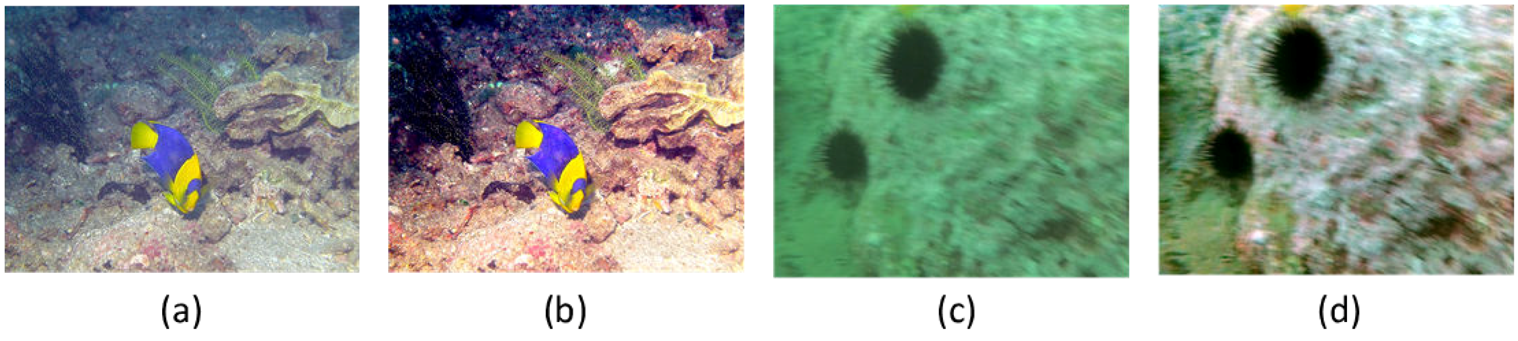
In this work, we adopted a simplified underwater imaging model which just considers the scattering and absorption of the light. Hence, our method could only address the degradation problems induced by scattering and absorption, such as contrast loss and color deviation. However, the real underwater imaging environment is actually very complicated. Some other factors, such as artificial light, water fluctuation and so on, are not taken into account in this simplified imaging model. Therefore, our method fails to properly recover the degraded images caused by these factors. Some failure examples are shown in Figure 15. When the underwater images are taken under the artificial light, our restoration results are prone to be over-compensated because of the incapability of removing the influence of artificial light. When processing the blurry underwater images induced by water fluctuation, our method can only correct the color cast and enhance the contrast, but fails to remove the blur.
To sum up, the imaging model we adopt is a simplified model in a quite ideal underwater environment which assumes imaging in a basically still water environment without artificial light. Thus, strictly speaking, our datasets synthesized by using this model, including training data and testing data, are not realistic enough, which may lead to an over-fitting. In the future work, we will refine the imaging model by considering more factors and build the dataset in a more reasonable way.
6. Conclusions
We have proposed an end-to-end CNN for underwater image restoration, accompanied by a new training dataset. Experimental results indicate that the proposed method can effectively restore natural color and increase contrast of underwater images.
In this work, we have adopted a simplified underwater optical imaging model, where some factors, such as the fluctuation of water, forward scattering and artificial light source are not taken into account. It is of considerable interest to study a more precise model, build a more realistic dataset, and design the corresponding deep-learning-based method.
Author Contributions
Methodology, Y.H., K.W. and X.Z.; software, Y.H.; validation, K.W. and Y.H.; investigation, Y.H. and K.W.; writing—original draft preparation, Y.H. and K.W.; writing—review and editing, K.W., J.C., Y.H. and X.W.; supervision, K.W.; project administration, K.W., X.W. and Y.L.; funding acquisition, X.W., K.W. and Y.L.
Funding
This work was supported in part by the China Postdoctoral Science Foundation (2013M540735), in part by the National Nature Science Foundation of China under Grant 61301291, 61701360, 61502367, 61501346, 61571345, 91538101, 61801359, 61401337, in part by the 111 Project under Grant B08038, in part by Yangtse Rive Scholar Bonus Schemes, in part by Ten Thousand Talent Program, and in part by the Fundamental Research Funds for the Central Universities.
Conflicts of Interest
The authors declare no conflict of interest.
References
- Mahiddine, A.; Seinturier, J.; Boï, D.P.J.; Drap, P.; Merad, D.; Long, L. Underwater image preprocessing for automated photogrammetry in high turbidity water: An application on the Arles-Rhone XIII roman wreck in the Rhodano river. In Proceedings of the 18th International Conference on Virtual Systems and Multimedia, Milan, Italy, 2–5 September 2012; pp. 189–194. [Google Scholar]
- Skarlatos, D.; Agrafifiotis, P.; Menna, F.; Nocerino, E.; Remondino, F. Ground control networks for underwater photogrammetry in archaeological excavations. In Proceedings of the 3rd IMEKO International Conference on Metrology for Archaeology and Cultural Heritage, Florence, Italy, 4–6 December 2019; pp. 23–25. [Google Scholar]
- Menna, F.; Agrafifiotis, P.; Georgopoulos, A. State of the art and applications in archaeological underwater 3D recording and mapping. J. Cult. Herit. 2018, 33, 231–248. [Google Scholar] [CrossRef]
- Čejka, J.; Bruno, F.; Skarlatos, D.; Liarokapis, F. Detecting Square Markers in Underwater Environments. Remote Sens. 2019, 11, 459. [Google Scholar] [CrossRef]
- Wang, X.; Li, Q.; Yin, J.; Han, X.; Hao, W. An Adaptive Denoising and Detection Approach for Underwater Sonar Image. Remote Sens. 2019, 11, 396. [Google Scholar] [CrossRef]
- Galdran, A.; Pardo, D.; Picón, A.; Gila, A. Automatic Red-Channel underwater image restoration. J. Vis. Commun. Image Represent. 2015, 26, 132–145. [Google Scholar] [CrossRef] [Green Version]
- Mangeruga, M.; Bruno, F.; Cozza, M.; Agrafiotis, P.; Skarlatos, D. Guidelines for Underwater Image Enhancement Based on Benchmarking of Different Methods. Remote Sens. 2018, 10, 1652. [Google Scholar] [CrossRef]
- Han, M.; Lyu, Z.; Qiu, T.; Xu, M. A Review on Intelligence Dehazing and Color Restoration for Underwater Images. IEEE Trans. Syst. Man Cybern. Syst. 2018, 99, 1–13. [Google Scholar] [CrossRef]
- Sun, L.; Wang, X.; Liu, X.; Ren, P.; Lei, P.; He, J.; Fan, S.; Zhou, Y.; Liu, Y. Lower-upper-threshold correlation for underwater range-gated imaging self-adaptive enhancement. Appl. Opt. 2016, 55, 8248–8255. [Google Scholar] [CrossRef]
- Henke, B.; Vahl, M.; Zhou, Z. Removing color cast of underwater images through non-constant color constancy hypothesis. In Proceedings of the International Symposium on Image and Signal Processing and Analysis, Trieste, Italy, 4–6 September 2013; pp. 20–24. [Google Scholar]
- Iqbal, K.; Odetayo, M.; James, A.; Salam, R.A.; Talib, A.Z. Enhancing the low quality images using Unsupervised Colour Correction Method. In Proceedings of the IEEE International Conference on Systems Man and Cybernetics, Istanbul, Turkey, 10–13 October 2010; pp. 1703–1709. [Google Scholar]
- Zhang, W.; Li, G.; Ying, Z. A New Underwater Image Enhancing Method via Color Correction and Illumination Adjustment. In Proceedings of the IEEE International Conference on Visual Communications and Image Processing, St. Petersburg, FL, USA, 10–13 December 2017; pp. 1–4. [Google Scholar]
- Fu, X.; Zhuang, P.; Huang, Y.; Liao, Y.; Zhang, X.; Ding, X. A retinex-based enhancing approach for single underwater image. In Proceedings of the IEEE International Conference on Image Processing, Paris, France, 27–30 October 2014; pp. 4572–4576. [Google Scholar]
- Zhang, S.; Wang, T.; Dong, J.; Yu, H. Underwater image enhancement via extended multi-scale Retinex. Neurocomputing 2017, 245, 1–9. [Google Scholar] [CrossRef] [Green Version]
- Ancuti, C.O.; Ancuti, C.; Haber, T.; Bekaert, P. Fusion-based restoration of the underwater imagespages. In Proceedings of the IEEE International Conference on Image Processing, Brussels, Belgium, 11–14 September 2011; pp. 1557–1560. [Google Scholar]
- Lu, H.; Li, Y.; Nakashima, S.; Kim, H.; Serikawa, S. Underwater Image Super-Resolution by Descattering and Fusion. IEEE Access 2017, 5, 670–679. [Google Scholar] [CrossRef]
- Ancuti, C.O.; Ancuti, C.; De Vleeschouwer, C.; Bekaert, P. Color Balance and Fusion for Underwater Image Enhancement. IEEE Trans. Image Process. 2018, 27, 379–393. [Google Scholar] [CrossRef]
- He, K.; Sun, J.; Tang, X. Single image haze removal using dark channel prior. IEEE Trans. Pattern Anal. Mach. Intell. 2011, 33, 2341–2353. [Google Scholar] [PubMed]
- Chiang, J.Y.; Chen, Y. Underwater image enhancement by wave-length compensation and dehazing. IEEE Trans. Image Process. 2012, 21, 1756–1769. [Google Scholar] [CrossRef] [PubMed]
- Drews, P., Jr.; Nascimento, E.R.; Botelho, S.S.C.; Campos, M.F.M. Underwater Depth Estimation and Image Restoration Based on Single Images. IEEE Comput. Graphics Appl. 2016, 36, 24–35. [Google Scholar] [CrossRef] [PubMed]
- Carlevaris-Bianco, N.; Mohan, A.; Eustice, R.M. Initial results in underwater single image dehazing. In Proceedings of the IEEE Conference on OCEANS, Seattle, WA, USA, 20–23 September 2010; Volume 27, pp. 1–8. [Google Scholar]
- Li, C.; Guo, J.; Pang, Y.; Chen, S. Single underwater image restoration by blue-green channels dehazing and red channel correction. In Proceedings of the IEEE International Conference on Acoustics, Speech and Signal Processing, Shanghai, China, 20–25 March 2016; pp. 1731–1735. [Google Scholar]
- Wang, N.; Zheng, H.; Zheng, B. Underwater Image Restoration via Maximum Attenuation Identification. IEEE Access 2017, 5, 18941–18952. [Google Scholar] [CrossRef]
- Li, C.; Guo, J.; Cong, R.; Pang, Y.; Wang, B. Underwater Image Enhancement by Dehazing With Minimum Information Loss and Histogram Distribution Prior. IEEE Trans. Image Process. 2016, 25, 5664–5677. [Google Scholar] [CrossRef] [PubMed]
- Berman, D.; Levy, D.; Avidan, S.; Treibitz, T. Underwater Single Image Color Restoration Using Haze-Lines and a New Quantitative Dataset. arXiv 2018, arXiv:1811.01343. [Google Scholar]
- Cai, B.; Xu, X.; Jia, K.; Qing, C.; Tao, D. DehazeNet: An End-to-End System for Single Image Haze Removal. IEEE Trans. Image Process. 2016, 25, 5187–5198. [Google Scholar] [CrossRef] [PubMed] [Green Version]
- Ren, W.; Liu, S.; Zhang, H.; Pan, J. Single Image Dehazing via Multi-scale Convolutional Neural Networks. In Proceedings of the European Conference on Computer Vision, Amsterdam, The Netherlands, 8–16 October 2016; pp. 154–169. [Google Scholar]
- Zhao, X.; Wang, K.; Li, Y.; Li, J. Deep Fully Convolutional Regres-sion Networks for Single Image Haze Removal. In Proceedings of the IEEE International Conference on Visual Communications and Image Processing, St. Petersburg, FL, USA, 10–13 December 2017; pp. 1–4. [Google Scholar]
- Shin, Y.; Cho, Y.; Pandey, G.; Kim, A. Estimation of ambient light and transmission map with common convolutional architecture. In Proceedings of the IEEE Conference on OCEANS, Monterey, CA, USA, 19–23 September 2016; pp. 1–7. [Google Scholar]
- Barbosa, W.V.; Amaral, H.G.B.; Rocha, T.L.; Nascimento, E.R. Visual-Quality-Driven Learning for Underwater Vision Enhancement. arXiv 2018, arXiv:1809.04624v1. [Google Scholar]
- Laina, I.; Rupprecht, C.; Belagiannis, V.; Tombari, F.; Navab, N. Deeper Depth Prediction with Fully Convolutional Residual Networks. In Proceedings of the IEEE Conference on 3D Vision, Stanford, CA, USA, 25–28 October 2016; pp. 239–248. [Google Scholar]
- Schechner, Y.Y.; Karpel, N. Clear underwater vision. In Proceedings of the IEEE Conference on Computer Vision and Pattern Recognition, Washington, DC, USA, 27 June–2 July 2004; pp. 1536–1543. [Google Scholar]
- Ren, W.; Ma, L.; Zhang, J.; Pan, J.; Cao, X.; Liu, W.; Yang, M. Gated Fusion Network for Single Image Dehazing. arXiv 2018, arXiv:1804.00213. [Google Scholar]
- Zhang, H.; Patel, V.M. Densely Connected Pyramid Dehazing Network. arXiv 2018, arXiv:1803.08396. [Google Scholar]
- He, K.; Sun, J.; Tang, X. Guided image filtering. IEEE Trans. Pattern Anal. Mach. Intell. 2013, 35, 1397–1409. [Google Scholar] [CrossRef] [PubMed]
- Scharstein, D.; Szeliski, R. High-Accuracy Stereo Depth Maps Using Structured Light. In Proceedings of the IEEE Conference on Computer Vision and Pattern Recognition, Madison, WI, USA, 16–22 June 2003; pp. 195–202. [Google Scholar]
- Scharstein, D.; Hirschmuller, H.; Kitajima, Y.; Krathwohl, G.; Nešić, N.; Wang, X.; Westling, P. High-Resolution Stereo Datasets with Subpixel-Accurate Ground Truth. In Proceedings of the German Conference on Pattern Recognition, Aachen, Germany, 7–10 October 2014; pp. 31–42. [Google Scholar]
- Liu, F.; Shen, C.; Lin, G. Deep convolutional neural elds for depth estimation from a single imagepages. In Proceedings of the IEEE Conference on Computer Vision and Pattern Recognition, Boston, MA, USA, 7–12 June 2015; pp. 5162–5170. [Google Scholar]
- Silberman, N.; Hoiem, D.; Kohli, P.; Fergus, R. Indoor Segmentation and Support Inference from RGBD Images. In Proceedings of the European Conference on Computer Vision, Florence, Italy, 7–13 October 2012; pp. 746–760. [Google Scholar]
- Li, B.; Ren, W.; Fu, D.; Tao, D.; Feng, D.; Zeng, W. RESIDE: A Benchmark for Single Image Dehazing. In Proceedings of the IEEE Conference on Computer Vision and Pattern Recognition, Honolulu, HI, USA, 21–26 July 2017. [Google Scholar]
- Wang, Z.; Bovik, A.C.; Sheikh, H.R.; Simoncelli, E.P. Image quality assessment: From error visibility to structural similarity. IEEE Trans. Image Process. 2004, 13, 600–612. [Google Scholar] [CrossRef] [PubMed]
- Luo, M.R.; Cui, G.; Rigg, B. The development of the CIE 2000 colour-difference formula: CIEDE2000. Color Res. Appl. 2001, 26, 340–350. [Google Scholar] [CrossRef]
- Mittal, A.; Moorthy, A.K.; Bovik, A.C. No-Reference Image Quality Assessment in the Spatial Domain. IEEE Trans. Image Process. 2012, 21, 4695–4708. [Google Scholar] [CrossRef] [PubMed]
- Yang, M.; Sowmya, A. An Underwater Color Image Quality Evaluation Metric. IEEE Trans. Image Process. 2015, 24, 6062–6071. [Google Scholar] [CrossRef] [PubMed]
Figure 1.
Examples of underwater images.

Figure 2.
The schematic diagram of underwater optical imaging.

Figure 3.
The architecture of our approach.

Figure 4.
The architecture of A-network.

Figure 5.
The architecture of T-network.

Figure 6.
Hue and brightness distribution of global ambient light. (a) the ambient light generated using a uniform distribution; (b) the ambient light generated using the modified distribution (note that the value of green-blue hue is 0.33–0.66).
Figure 6.
Hue and brightness distribution of global ambient light. (a) the ambient light generated using a uniform distribution; (b) the ambient light generated using the modified distribution (note that the value of green-blue hue is 0.33–0.66).

Figure 7.
The comparison results. (a) underwater images; (b) the restored images based on the dataset generated without the modified ambient light distribution; (c) the restored images based on the dataset generated using the modified ambient light distribution.
Figure 7.
The comparison results. (a) underwater images; (b) the restored images based on the dataset generated without the modified ambient light distribution; (c) the restored images based on the dataset generated using the modified ambient light distribution.

Figure 8.
Training and validation loss over the training process. (a) loss of A-network; (b) loss of T-network.
Figure 8.
Training and validation loss over the training process. (a) loss of A-network; (b) loss of T-network.

Figure 9.
Comparison of different methods on synthetic underwater images. (a) the input synthetic underwater images; (b) the results of Drews et al. [20]; (c) the results of Li et al. [24]; (d) the results of Berman et al. [25]; (e) the results of Shin et al. [29]; (f) our results without the guided filter; (g) our results with the guided filter; (h) the ground truth clear images.

Figure 10.
Comparisons of the restored images and their corresponding estimated blue-channel transmission and ambient light by different methods. Each ambient light is visualized as a colored bar for the convenience of comparison. (a) the input synthetic underwater images; (b) the results of Drews et al. [20]; (c) the results of Li et al. [24]; (d) the results of Berman et al. [25]; (e) the results of Shin et al. [29]; (f) our results without the guided filter; (g) our results with the guided filter; (h) the ground truth clear images.

Figure 11.
Visual comparison for recovered results on real-world underwater images. (a) underwater images; (b) the results of Fu et al. [13]; (c) the results of Zhang et al. [12]; (d) the results of Drews et al. [20]; (e) the results of Li et al. [24]; (f)the results of Berman et al. [25]; (g) the results of Shin et al. [29]; (h) the results of the proposed method.

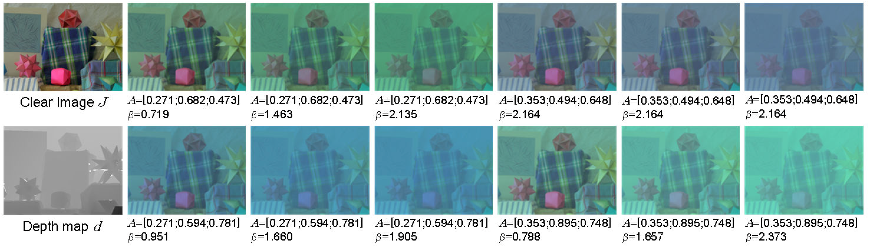
Figure 12.
Synthetic samples. The images in the first column are from Middlebury Stereo dataset. The others are synthetic underwater images with different global ambient light and blue channel attenuation coefficients.
Figure 12.
Synthetic samples. The images in the first column are from Middlebury Stereo dataset. The others are synthetic underwater images with different global ambient light and blue channel attenuation coefficients.

Figure 13.
Comparisons on the estimated ambient light and restoration results. Each ambient light is visualized as a colored bar for the convenience of comparison. (a) underwater images; (b) the results of Shin et al. [29]; (c) the results of the proposed method.
Figure 13.
Comparisons on the estimated ambient light and restoration results. Each ambient light is visualized as a colored bar for the convenience of comparison. (a) underwater images; (b) the results of Shin et al. [29]; (c) the results of the proposed method.

Figure 14.
Transmission map estimation results using different modules. (a) underwater images; (b) ground truth; (c) U-shaped structure (DFCRN); (d) U-shaped structure + multi-scale estimation; (e) U-shaped structure + multi-scale estimation + cross layer connection(our T-network).
Figure 14.
Transmission map estimation results using different modules. (a) underwater images; (b) ground truth; (c) U-shaped structure (DFCRN); (d) U-shaped structure + multi-scale estimation; (e) U-shaped structure + multi-scale estimation + cross layer connection(our T-network).

Figure 15.
Some failure examples. (a) an underwater image taken under the artificial light; (b) our result; (c) a blurry underwater image induced by water fluctuation; (d) our result.
Figure 15.
Some failure examples. (a) an underwater image taken under the artificial light; (b) our result; (c) a blurry underwater image induced by water fluctuation; (d) our result.


Table 1.
Method to generate .
| Distribution | Ratio |
|---|---|
| ; | 6 |
| ; | 2 |
| ; | 1 |
| ; | 1 |
© 2019 by the authors. Licensee MDPI, Basel, Switzerland. This article is an open access article distributed under the terms and conditions of the Creative Commons Attribution (CC BY) license (http://creativecommons.org/licenses/by/4.0/).
Share and Cite
MDPI and ACS Style
Wang, K.; Hu, Y.; Chen, J.; Wu, X.; Zhao, X.; Li, Y. Underwater Image Restoration Based on a Parallel Convolutional Neural Network. Remote Sens. 2019, 11, 1591. https://0-doi-org.brum.beds.ac.uk/10.3390/rs11131591
AMA Style
Wang K, Hu Y, Chen J, Wu X, Zhao X, Li Y. Underwater Image Restoration Based on a Parallel Convolutional Neural Network. Remote Sensing. 2019; 11(13):1591. https://0-doi-org.brum.beds.ac.uk/10.3390/rs11131591
Chicago/Turabian StyleWang, Keyan, Yan Hu, Jun Chen, Xianyun Wu, Xi Zhao, and Yunsong Li. 2019. "Underwater Image Restoration Based on a Parallel Convolutional Neural Network" Remote Sensing 11, no. 13: 1591. https://0-doi-org.brum.beds.ac.uk/10.3390/rs11131591
Note that from the first issue of 2016, this journal uses article numbers instead of page numbers. See further details here.