Article

Using Digital Cameras on an Unmanned Aerial Vehicle to Derive Optimum Color Vegetation Indices for Leaf Nitrogen Concentration Monitoring in Winter Wheat

1
National Engineering and Technology Center for Information Agriculture, Nanjing Agricultural University, Nanjing 210095, China
2
Key Laboratory for Crop System Analysis and Decision Making, Ministry of Agriculture, Nanjing Agricultural University, Nanjing 210095, China
3
Jiangsu Key Laboratory for Information Agriculture, Nanjing Agricultural University, Nanjing 210095, China
4
Jiangsu Collaborative Innovation Center for Modern Crop Production, Nanjing Agricultural University, Nanjing 210095, China
5
School of Engineering, University of California, 5200 Lake Road, Merced, CA 95343, USA
6
Qinghai Science and Technology Information Research Institute Co. LTD, Qinghai 810000, China
*
Author to whom correspondence should be addressed.
Remote Sens. 2019, 11(22), 2667; https://0-doi-org.brum.beds.ac.uk/10.3390/rs11222667
Submission received: 29 September 2019 / Revised: 11 November 2019 / Accepted: 13 November 2019 / Published: 14 November 2019
(This article belongs to the Special Issue Remote Sensing for Precision Nitrogen Management)

Abstract

:
Commercially available digital cameras can be mounted on an unmanned aerial vehicle (UAV) for crop growth monitoring in open-air fields as a low-cost, highly effective observation system. However, few studies have investigated their potential for nitrogen (N) status monitoring, and the performance of camera-derived vegetation indices (VIs) under different conditions remains poorly understood. In this study, five commonly used VIs derived from normal color (RGB) images and two typical VIs derived from color near-infrared (CIR) images were used to estimate leaf N concentration (LNC). To explore the potential of digital cameras for monitoring LNC at all crop growth stages, two new VIs were proposed, namely, the true color vegetation index (TCVI) from RGB images and the false color vegetation index (FCVI) from CIR images. The relationships between LNC and the different VIs varied at different stages. The commonly used VIs performed well at some stages, but the newly proposed TCVI and FCVI had the best performance at all stages. The performances of the VIs with red (or near-infrared) and green bands as the numerator were limited by saturation at intermediate to high LNCs (LNC > 3.0%), but the TCVI and FCVI had the ability to mitigate the saturation. The results of model validations further supported the superiority of the TCVI and FCVI for LNC estimation. Compared to the other VIs derived using RGB cameras, the relative root mean square errors (RRMSEs) of the TCVI were improved by 8.6% on average. For the CIR images, the best-performing VI for LNC was the FCVI (R2 = 0.756, RRMSE = 14.18%). The LNC–TCVI and LNC–FCVI were stable under different cultivars, N application rates, and planting densities. The results confirmed the applicability of UAV-based RGB and CIR cameras for crop N status monitoring under different conditions, which should assist the precision management of N fertilizers in agronomic practices.

Graphical Abstract

1. Introduction

Nitrogen (N) is a component of many important compounds in plants, and thus plays an important role in plant growth [1,2]. Plant growth dominantly depends on the N supply [3]. A deficiency in N would reduce crop photosynthesis, whereas higher rates of N fertilization do not necessarily improve crop yield and can lead to serious water pollution [4,5,6]. Furthermore, leaf N concentration (LNC) is related to the photosynthetic capacity of leaves, and thus allows N fertilizer applications and grain quality to be modeled [7,8]. Therefore, timely quantification of LNC is a prerequisite for fertilization guidance and environmental quality [9,10].
Unmanned aerial vehicle (UAV) platforms have become a promising approach in precision agricultural assessments because they enable the non-destructive measurement of crop growth status, with a very high spatio-temporal resolution [11,12]. Due to their advantages of low cost, light weight, convenient operation, and simple data processing, digital cameras have been commonly deployed on UAVs in crop phenotype research [13]. Compared to other sensors, digital cameras can operate successfully in a range of working environments. Given that adequate image exposure can be set based on the weather conditions, data can be collected under both sunny and cloudy conditions [13]. Therefore, color images can be instantly acquired for researchers and farmers to monitor crop growth status [14].
A consumer-grade RGB camera is an “off-the-shelf” device, with red, green, and blue channels. Because each pixel value in color images can be calculated from the digital number (DN) values of specific bands, color indices can be extracted to accentuate a particular vegetation greenness and identify the vegetation features [14,15]. Hunt et al., [16] used the normalized green–red difference index (NGRDI) from RGB images to estimate the biomass of corn, alfalfa, and soybean, and found a linear correlation between the NGRDI and biomass. Kawashima and Nakatani [17] used a video camera to analyze the color of wheat leaves for estimating chlorophyll content. Woebbecke et al. [18] investigated the capability of several color indices to distinguish vegetation from the background, and found that the excess green vegetation index (ExG) could provide a near-binary intensity image outlining a plant region of interest. Moreover, color indices from RGB cameras containing a large amount of information regarding crop status can be used to estimate the vegetation fraction, plant height, biomass, and yield [19,20,21]. However, many vegetation indices (VIs) proposed for crop status monitoring contain the near infrared (NIR) bands [22,23,24]. Therefore, RGB cameras with a Bayer-pattern array of filters have been modified by replacing either the blue or red channel with a NIR channel to obtain color near-infrared (CIR) images [25]. Based on a newly-developed digital CIR camera system, Hunt et al., [25] found a strong correlation between the green normalized difference vegetation index (GNDVI) and leaf area index (LAI) in winter wheat. This CIR camera system has also been used to assess winter crop biomass [26]. Four VIs, the normalized difference vegetation index (NDVI), enhanced NDVI (ENDVI), GNDVI, and ExG, derived from UAV-based RGB and CIR images, have been shown to be reliable to assess experimental plots [27].
Previous studies have indicated that it is feasible to estimate crop growth status using RGB and CIR images, but few studies have investigated their usability for N status monitoring [12,28]. Firstly, the capability of digital cameras to monitor wheat LNC at different growth stages remains poorly understood. Since the composition of canopy components (e.g., leaves, tassels) and background materials (e.g., soil) varied sharply during whole growth stages of winter wheat [29], the performance of digital cameras on estimating LNC is necessary to be tested across different growth stages. Secondly, it is crucial to investigate the saturation problem of VIs, with varying LNC values. Because the application of N fertilizer has increased recently in China, it is important to effectively monitor LNC under middle to high application levels. Thirdly, the capability of digital cameras for LNC estimation under different conditions is unclear. The relationships among VIs and LNC in cereal crops have been investigated in terms of the mechanisms involved based on hyperspectral remote sensing. Many studies have proposed effective VIs that can be adjusted to variations in growth stage [30] and geographic location [31], and that can reduce the effects of the soil background [32]. Therefore, there is also a need to assess the capability of digital cameras for estimating wheat LNC under different conditions.
The overall objective of this study was to evaluate whether digital cameras mounted on UAVs could be applied to monitor LNC in winter wheat. Five typical VIs derived from RGB images and two widely used VIs derived from CIR images were selected to estimate LNC. Additionally, we developed the true color vegetation index (TCVI) and the false color vegetation index (FCVI) from RGB and CIR images, respectively. Experiments with different wheat varieties, planting densities, and N application rates were conducted in the field to: (1) quantify the relationship between LNC and the VIs from digital imagery at different growth stages, (2) evaluate the saturation sensitivity of the VIs under various LNC levels, and (3) validate the applicability of the LNC estimation models under different treatments.

2. Materials and Methods

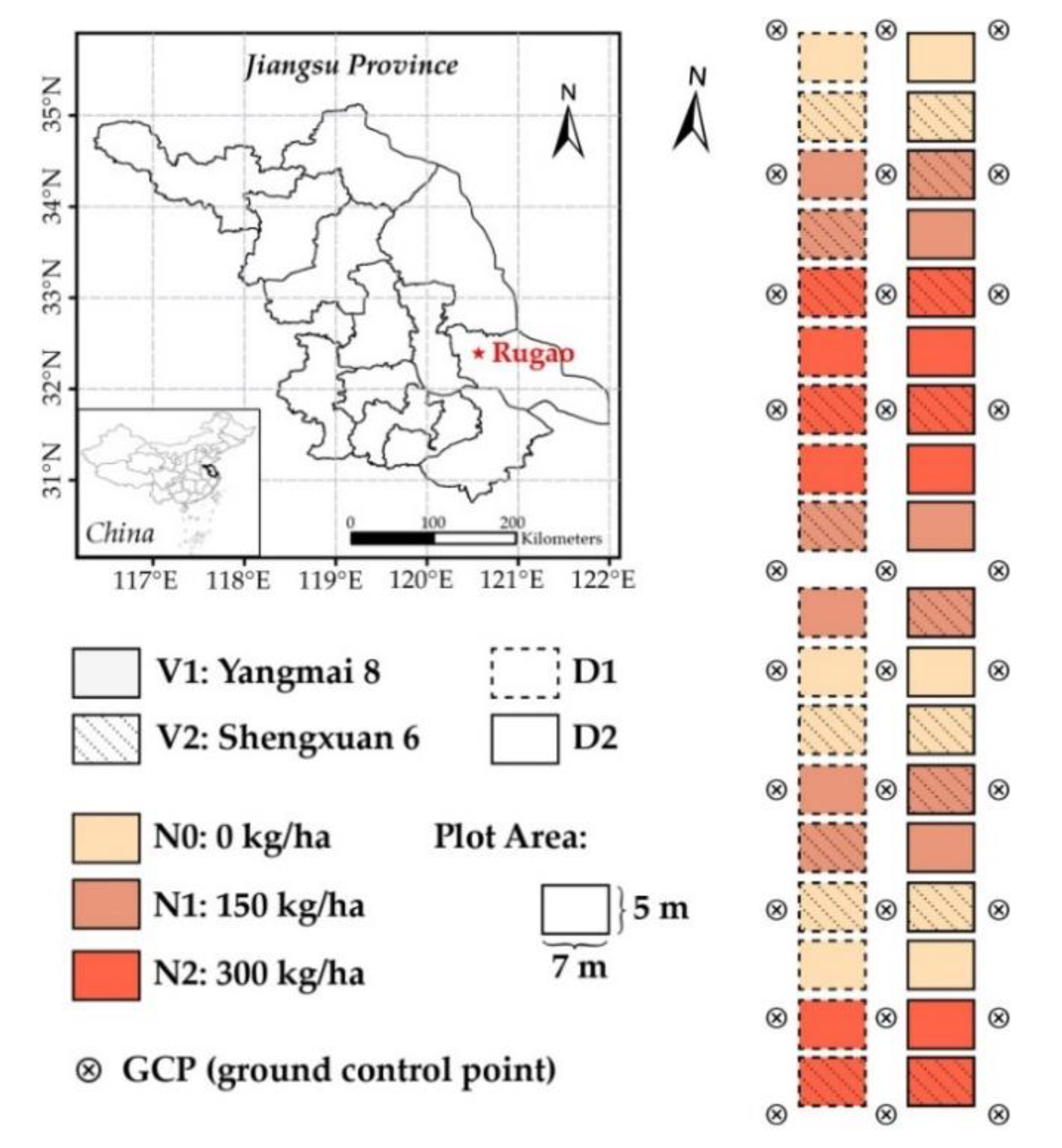
2.1. Study Site and Experimental Design

The study site was located in Rugao City, Jiangsu Province, China (120°45′ E, 32°16′ N), as shown in Figure 1. The regional annual precipitation of this area is around 927.53 mm, with an average annual temperature of 16.59 °C. Two field experiments using winter wheat (Triticum aestivum L.) were designed that included three N application rates, two planting densities (D), and two varieties (V) in two growing seasons (Table 1). In each experiment, a split design was used with three replications and there were 36 plots, each with a plot area of 35 m2 (Figure 1). The basal fertilizer included 120 kg/ha P2O5 and 120 kg/ha K2O and there were three N application rates (0, 150, and 300 kg/ha as urea) applied at the end of October 2013/2014. Compound fertilizer was applied in early March 2014/2015, including N applications at the three different rates. The N fertilizers were applied in 50% as basal fertilizer at the sowing day and in 50% at the jointing stage. All other agronomic management was undertaken according to local wheat production practices.

2.2. Data Acquisition and Processing

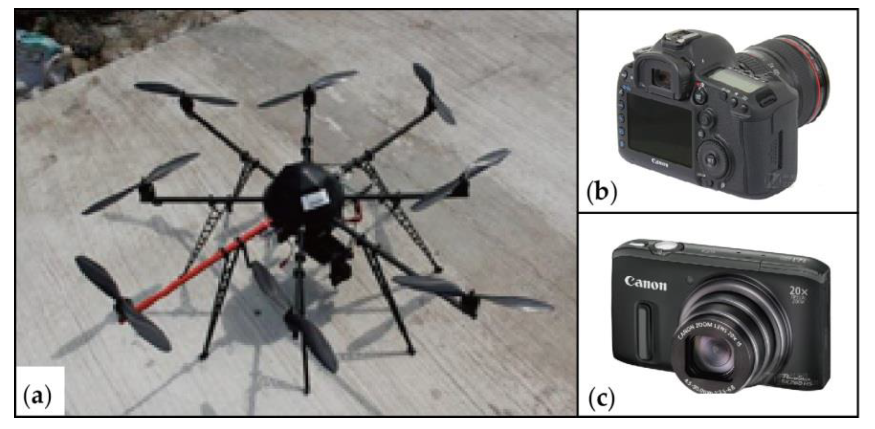
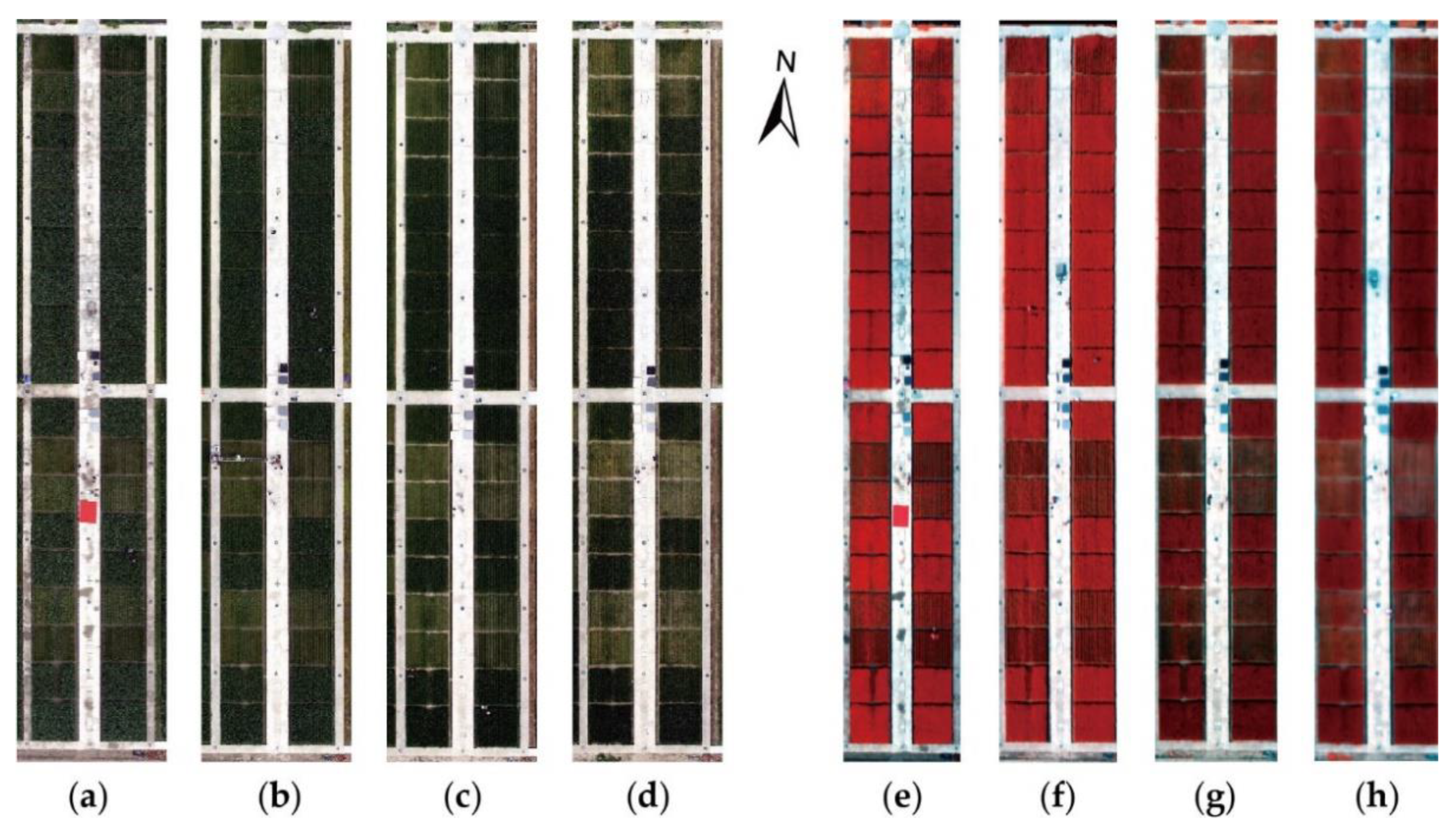
2.2.1. Color Images from Unmanned Aerial Vehicle (UAV)

In this study, an eight-rotor ARF-MikroKopter UAV (Figure 2a) was used as the platform for the UAV-camera system and its specifications are listed in Table 2. A Canon 5D Mark III (Canon Inc., Japan) commercial digital camera (Figure 2b) was mounted on the UAV and took RGB images in continuous mode. The CIR camera was modified from a Canon SX260HS camera (Canon Inc.) by changing the original red channel to a near-infrared channel. The main parameters of the two cameras are described in Table 3. An MC-32 remote control module and a ThinkPad laptop were used to control the autonomous UAV flight. During each flight, the camera was fixed on a two-axis gimbal, with the lens positioned vertically downward at 50 m altitude. Considering the lighting conditions, the exposure time and shutter speed were fixed for each campaign. UAV campaigns were conducted at noon in clear weather under stable light conditions. The spatial resolution of the RGB and CIR imagery was 3 cm. The acquisition dates of these images are listed in Table 4.
Before image pre-processing, the original digital images were screened. We selected images with a heading overlap rate of ~70% and a side overlap rate of ~30%, and excluded images with excessive repetition. The selected images were then pre-processed, including a lens distortion correction, image mosaicking, image registration, and ortho-rectification. First, lens distortion was corrected based on the Brown Model and the correction coefficients were calculated by an Agisoft Lens. Second, image mosaicking was conducted in Photoscan (Airsoft LLC, Russia). Third, image registration was referred to ground control points (GCPs) in the experimental area (see Figure 1). The GCPs were painted on a road surface as black annuluses, with inner and outer diameters of 10 and 50 cm, respectively. The geographic coordinates of the GCPs were determined using a real time kinematic (RTK) GPS system, with an error less than 2 cm in the horizontal direction and less than 3 cm in the vertical direction. Finally, ortho-rectification was automatically performed using Photoscan. Figure 3 shows the processed images from RGB and CIR cameras at the four growth stages.

2.2.2. Determination of Leaf N Concentration (LNC)

Common measures of crop LNC are either area-based (LNCarea, g/m2) or mass-based (LNCmass, %). LNCarea is the N mass per unit leaf area and LNCmass is the ratio of N mass to leaf dry mass. These two measures can be converted between each other through the leaf mass per area (LMA), i.e., LNCarea = LNCmass × LMA [33]. Therefore, LNCarea should be determined based on both LNCmass and LMA measures, while LNCmass can be measured directly in the laboratory. Given its strong connection with photosynthetic capacity [34] and its widespread use in fertilization management [35,36], LNCmass has received more attention and has been estimated from remotely sensed data more often than its counterpart LNCarea [37,38,39,40]. The term LNC hereafter refers to LNCmass.
Ground destructive samplings were taken at critical growth stages of winter wheat (Table 1) on the same dates as the UAV campaigns. Thirty hills of wheat plants were randomly cut above the ground surface of each plot and separated into leaves, stems, and panicles. All leaves were oven-dried at 105 °C for 30 min and then at 80 °C until a constant weight. We then grounded and stored all samples in plastic bags for chemical analysis. The LNC was determined based on the micro-Keldjahl method [41] with SEAL AutoAnalyzer 3 HR (SEAL Analytical, Ltd., German).

2.2.3. Derivation of Vegetation Indices (VIs)

The main VIs derived from digital camera images are summarized in Table 5. For RGB cameras, five widely used color indices were chosen in this study: the NGRDI [42], Kawashima index (IKaw) [17], red green ratio index (RGRI) [43], visible atmospherically resistance index (VARI) [42], and ExG [18]. For the CIR camera, we used the GNDVI [44] and enhanced normalized difference vegetation index (ENDVI), because GNDVI is related to chlorophyll concentration, while the ENDVI was recommended by the company that manufactured the modified cameras (www.maxmax.com) and also can monitor vegetation vigor [27]. The VIs could be categorized into two groups according to the number of channels used. Some were constructed by two channels, such as NGRDI, IKaw, RGRI, and GNDVI. The others (i.e., VARI, ExG, and ENDVI) were established using three channels.
Color vegetation index (CVI) derived from digital imagery is often calculated as ratios of DN values. However, the previous VIs listed in Table 5 were proposed without considering background material, such as soil in the field. Previous studies have suggested that the influence of the soil background can be reduced by adjusting the VIs with a term representing soil brightness [22,28]. Based on the ratio form and an equivalent soil adjustment, the commonly used CVIs from digital cameras can be expressed as:
C V I = ( 1 + L ) ( a 1 R + a 2 G + a 3 B ) ( a 4 R + a 5 G + a 6 B + 255 L )
where G and B are the DN values of the green and blue channels, respectively; R represents the red component of RGB imagery or the near-infrared component of CIR imagery; ai is the coefficient of each channel; and L is a soil background adjustment parameter.
To explore the capability of digital cameras for estimating LNC in wheat, we constructed new CVI from both RGB and CIR images. They were determined by optimizing the values of ai and L based on the cost function J defined as:
J = 1 i = 1 n ( L N C m , i L N C p , i ) 2 i = 1 n ( L N C m , i L N C m , i ¯ ) 2
where LNCm is the measured LNC. LNCp was predicted by the best fitted function of CVI and L N C p ¯ is the average value of LNCp. According to the imaging principle of a Bayer filter, we set the value of ai as an element of {−2, −1, 0, 1, 2}. Based on the setting rules of a soil background adjustment parameter in [22], L ranges from 0 to 1, with intervals of 0.1. The value of L varies by the amount or cover of green vegetation: in very high vegetation regions, L = 0; and in areas with no green vegetation, L = 1. Given that the maximum value of the DN was 255, L was multiplied by 255 in the denominator. All data from Exp. 2 were used in Equation (2). All possible combinations of variables (i.e., ai and L) were traversed, and the corresponding values of J were compared. The values of ai and L in Equation (1) that yield the best J were the optimal variables. Consequently, the TCVI from RGB images and the FCVI from CIR images were determined as follows:
T C V I = ( 1 + 0.4 ) ( 2 R 2 B ) ( 2 R G 2 B + 255 0.4 )
F C V I = ( 1 + 0.5 ) ( 2 N I R + B 2 G ) ( 2 G + 2 B 2 N I R + 255 0.5 )

2.3. Data Analysis and Evaluation

The channel information from digital cameras that constituted the VIs was first analyzed based on the data from Exp. 2. We analyzed how the DN values of different channels changed with the changes of LNC in wheat. To compare and evaluate the performances of different VIs for estimating LNC, the quantitative relationship between the VIs and LNC was analyzed at different growth stages. For all growth stages of winter wheat, the LNC–VI models from both RGB and CIR images were calibrated and validated with a 10-fold cross-validation procedure using the data from Exp. 2. The whole dataset was randomly divided into three equal-sized sub-datasets with two sub-datasets used as the calibration (training) dataset and the rest as the validation (testing) dataset. The process was repeated 10 times [45]. For the CIR cameras, the estimation models were also validated independently with the data from Exp. 1. The performance of the different VIs and models were evaluated using the determination coefficient (R2) and the relative root mean square error (RRMSE).
R 2 = 1 i = 1 n ( O i P i ) 2 i = 1 n ( O i O i ¯ ) 2
R R M S E = 1 n i 1 n ( O i P i ) 2 × 1 O i ¯ × 100 %
where n is the number of samples; Oi is the observed LNC value; and Pi is the estimated value. The saturation sensitivity of the VI versus LNC was evaluated using the index of noise equivalent (NE△LNC) [46,47].
N E Δ L N C = R M S E { V I v s . L N C } d ( V I ) / d ( L N C )
where RMSE{VIvs.LNC} is the root mean square error (RMSE) of the best fit function and the actual LNC value, and d(VI)/d(LNC) is the first derivative of VI with respect to LNC. A higher NE△LNC indicates a lower sensitivity to LNC. The accuracies of the optimal estimation models from RGB and CIR images were compared under different treatments (i.e., different varieties, N application rates, and planting densities) using RRMSE.

3. Results

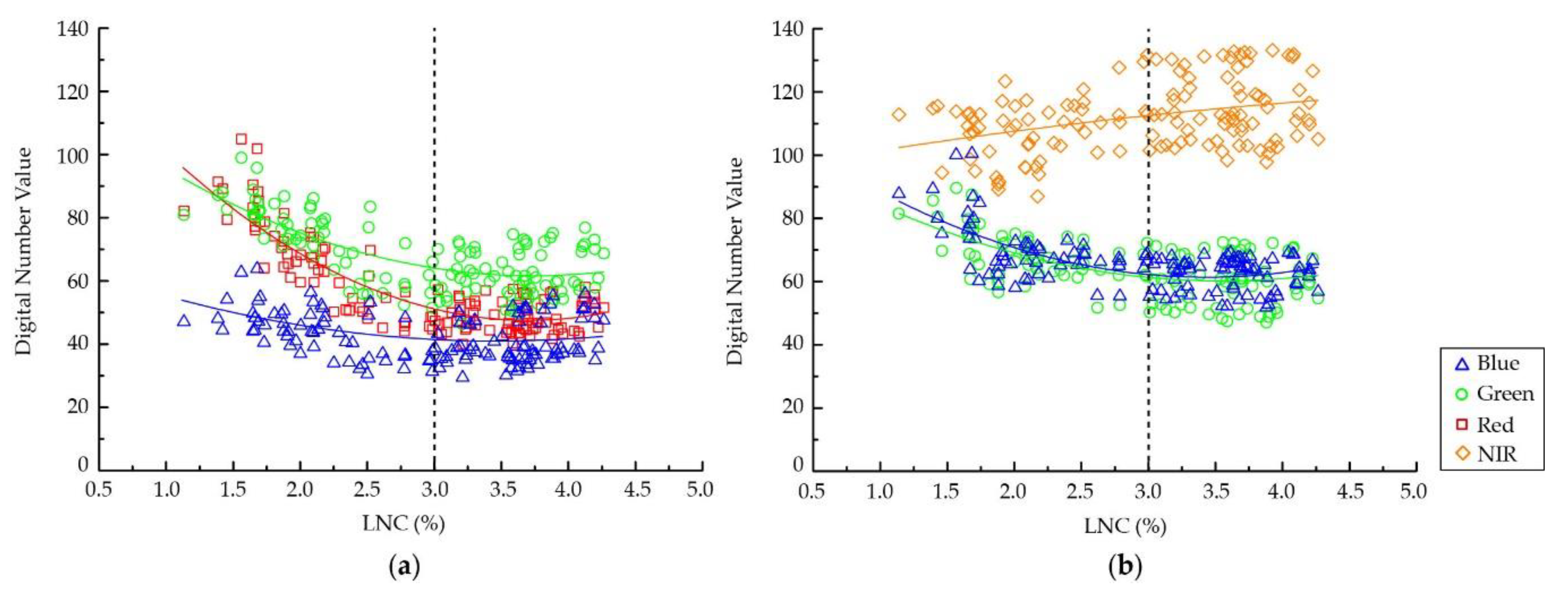
3.1. Changes of Digital Number (DN) Values in Different Channels

Figure 4 shows the changes of DN values in different channels with the variation in LNC for images from the RGB and CIR cameras. The DN values of all channels from the RGB camera decreased when the LNC increased to 3.0%, and then became flatter as the LNC continually increased (Figure 4a). Conversely, the DN values of the near infrared channel from the CIR camera increased as the LNC increased (Figure 4b). The variations of the DN values in the blue and green channels from both cameras were similar, but the values were different. For the RGB camera, the values of the green channel were higher than those of the blue channel. For the CIR camera, the DN values of the green and blue channels were similar.

3.2. Leaf N Concentration (LNC) Estimation Model Constraction and Validation

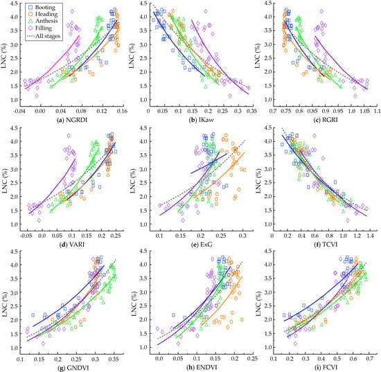
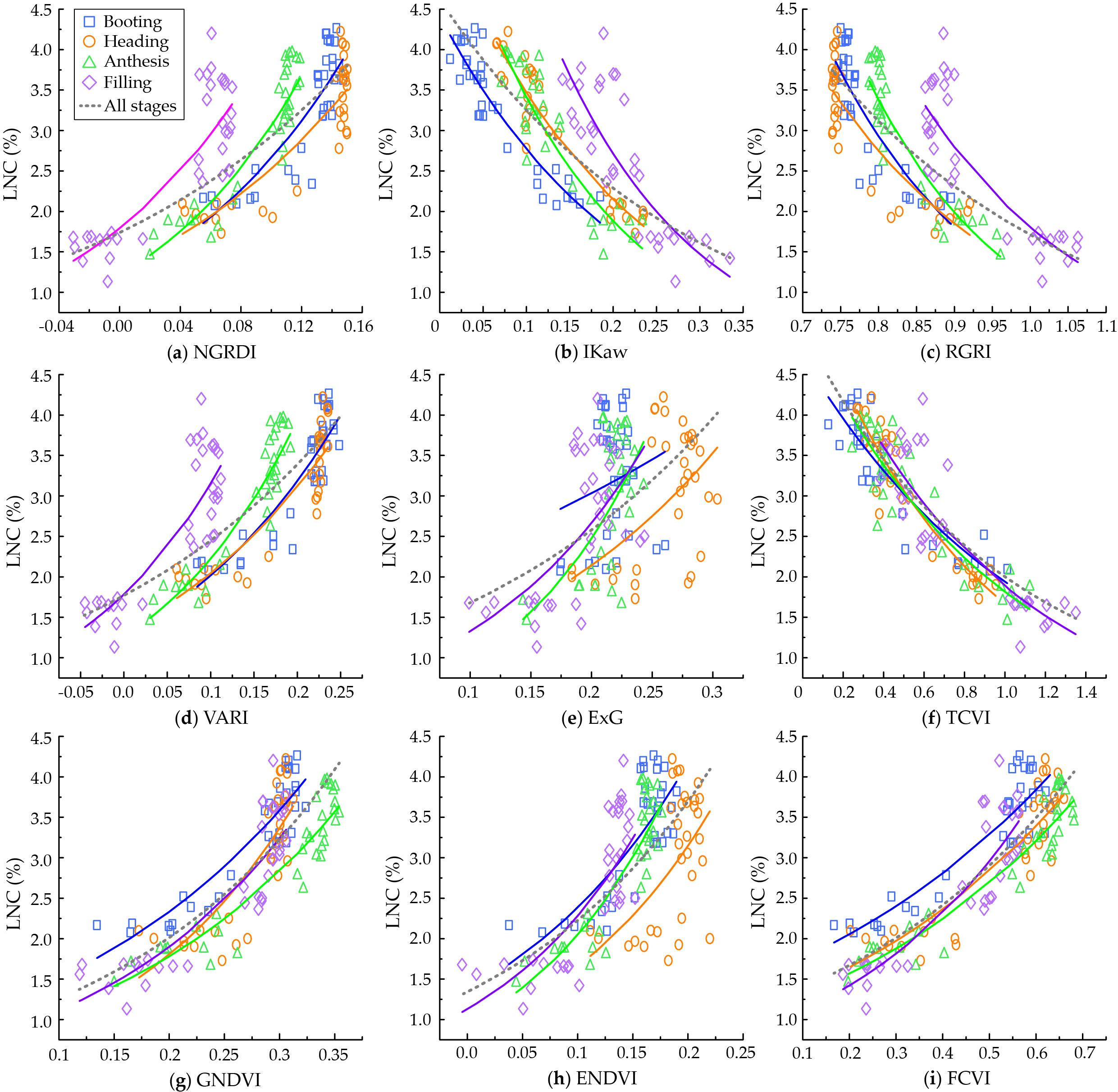
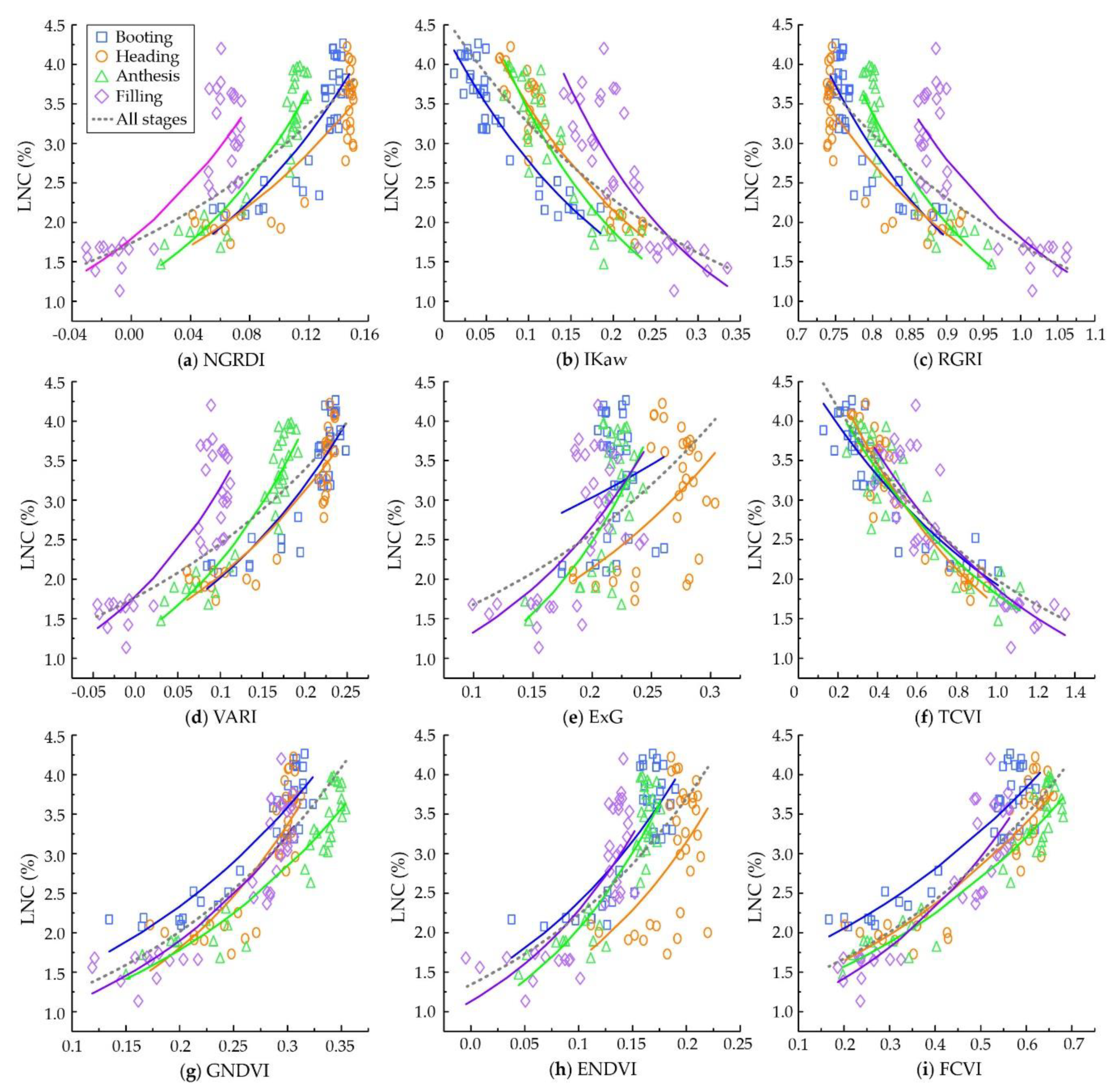
3.2.1. Quantitative Relationships between Leaf N Concentration (LNC) and Vegetation Indices (VIs) at Different Growth Stages

Figure 5 shows the relationship between LNC and the VIs determined from both RGB and CIR images at different growth stages of winter wheat. For the VIs derived from RGB images, the results were quite different (Figure 5a–f). When the LNC increased, the NGRDI, VARI, and ExG increased, while the IKaw, RGRI, and TCVI decreased. The exponential relationship between the ExG and LNC was weak at all four stages (Figure 5e). The relationship between the NGRDI and LNC (Figure 5a) was similar to that between the VARI and LNC, but the fitting curves of the VARI and LNC at the booting and heading stages were stronger than those of the NGRDI and LNC (Figure 5d). Unlike the other VIs, the relationship between the TCVI and LNC was almost identical at all four stages (Figure 5f). For the VIs derived from CIR images, the GNDVI, ENDVI, and FCVI all increased as the LNC increased (Figure 5g–i). The results for the GNDVI and FCVI at each growth stage were similar (Figure 5g,i). The sample points for the relationship between the ENDVI and LNC were distributed along the fitting curves at the booting, anthesis, and filling stages, but at the heading stage the results were scattered (Figure 5h). At intermediate to high LNC levels, the NGRDI, RGRI, VARI, and GNDVI were not sensitive to changes in LNC > 3.0%, especially at the heading stage.
To quantitatively analyze the ability of the VIs to estimate LNC at different growth stages, the R2 and RRMSE values at each growth stage and over all four stages are listed in Table 6. Generally, the results at the filling stage were much worse than at the other three stages, with an RRMSE higher than 15%. In the first three stages, the RRMSE values of most VIs were around 10%. However, the performances of the ExG and ENDVI were much poorer than those of the other VIs, especially at the heading and filling stages. The results for the TCVI and FCVI were not remarkably better than the other VIs at each growth stage, but they were obviously better for all four stages combined. For the RGB camera, the IKaw performed best at the booting and heading stages, and the VARI had the highest R2 and lowest RRMSE values at the anthesis stage. Although the TCVI results were not the most accurate in the first three stages, they were superior to those of the other VIs derived from RGB images at the filling stage. For the CIR camera, the performance of the ENDVI was much poorer than that of the GNDVI and FCVI. The FCVI performed best at each stage, although the RRMSE of 9.5% at the booting stage was slightly higher than the value of 9.1% for the GNDVI. Compared to the VIs from RGB images, the FCVI results were less accurate than those of the IKaw at the first two stages, but were the most accurate at the anthesis and filling stages. For all four stages combined, the performance of the TCVI was remarkable, with an R2 value of 0.852 and RRMSE of 12.1%, followed by the FCVI with an R2 value of 0.792 and RRMSE of 14.0%.

3.2.2. Validation of the Leaf N Concentration (LNC) Models for Wheat

The validation statistics for the LNC models constructed from the different VIs are presented in Table 7. According to the results of the 10-fold cross-validation, the estimation models constructed from the TCVI had the highest accuracy. Compared to the other VIs from the RGB camera, the RRMSEs were improved by 6.32% to 15.76% for LNC based on the TCVI. For CIR images, the statistical values of the FCVI were the best for LNC, followed by the GNDVI. The independent validation indicated that the FCVI was capable of producing accurate LNC estimations at all stages.

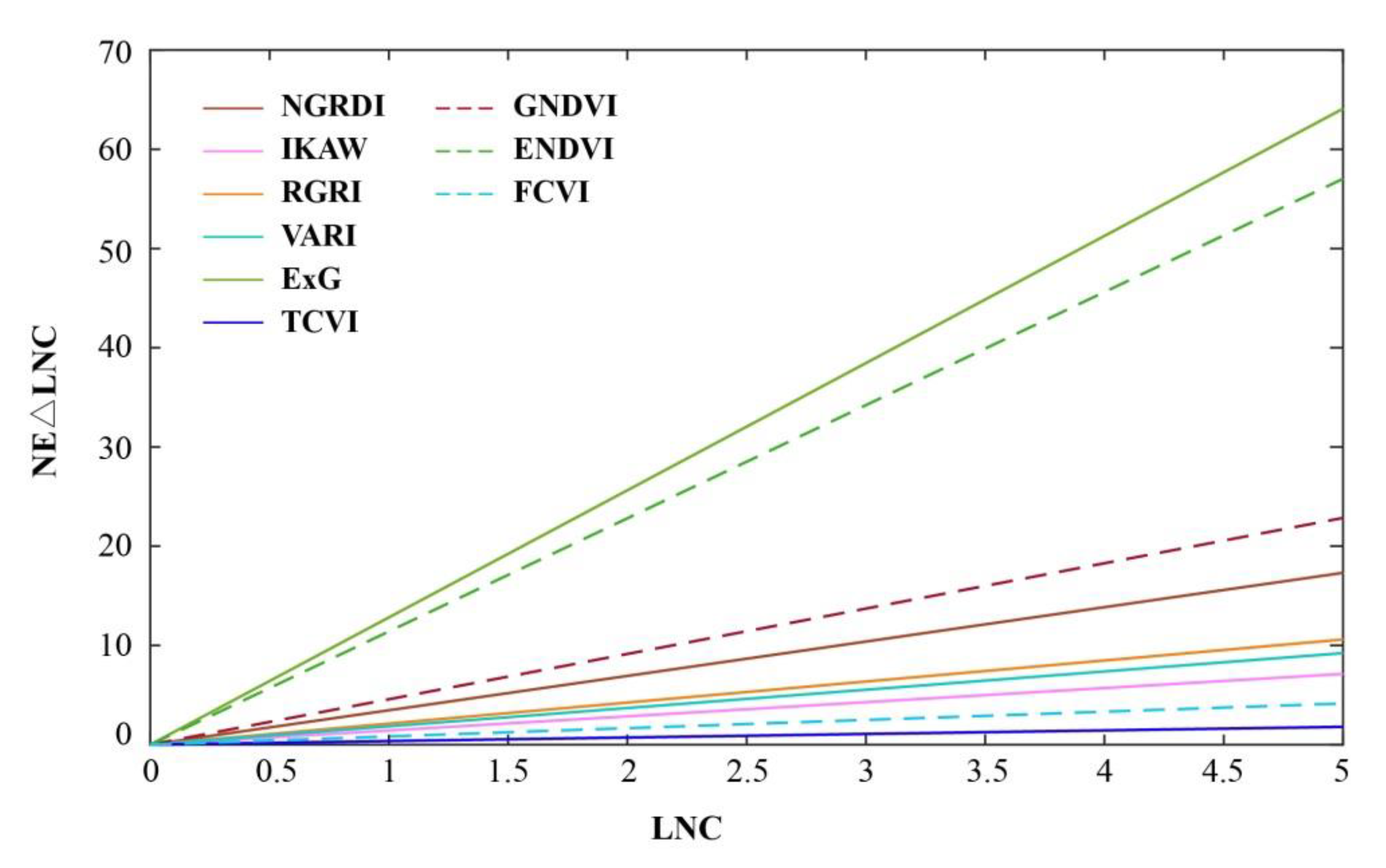
3.3. Saturation Sensitivity of Vegetation Indices (VIs) at Different Leaf N Concentrations (LNCs)

As shown in Figure 6, the saturation of the selected VIs was tested under the LNC range of 0 to 5%. The NE△LNC of ExG increased sharply as the LNC increased. The ExG was the VI with the fastest and largest increase, followed by the ENDVI. When LNC < 3%, the NE△LNC of the IKAW, RGRI, and VARI were similar. However, when LNC > 3%, the NE△LNC of the IKAW increased more slowly than that of the RGRI and VARI. Compared to the other VIs, the NE△LNC of the TCVI and FCVI were much lower, with that of the TCVI being the smallest. The NE△LNC of the TCVI was still the lowest of all the VIs at high LNCs.

3.4. Applicability of the Leaf N Concentration (LNC) Models under Different Treatments

According to the results in Table 6, the optimal LNC estimation models for the whole season from RGB and CIR images were constructed by the TCVI and FCVI, respectively. Table 8 shows a comparison of the optimal estimation models from RGB and CIR images under the different treatments. Generally, the RRMSE values of LNC estimations under the various treatments were lower than 15%.
For the different wheat varieties, the RRMSE values of LNC estimations from RGB images were lower than those from CIR images, with the lowest RRMSE of 9.88% for Shengxuan 6. Under the different N application rates, the LNC models from RGB images performed better than those from CIR images. For both RGB and CIR images, the RRMSE values for N application rates of 150 kg/ha were lower than for the other N application rates. As planting density decreased, the accuracy of LNC estimation from RGB images decreased, while for CIR images it increased. The best results for the lowest planting density were obtained from CIR images, and the lowest RRMSE values for the highest planting density were obtained from RGB images.

4. Discussion

4.1. Performance of the Vegetation Indices (VIs) Derived from Digital Imagery in Estimating Wheat Leaf N Concentration (LNC)

The estimation of VIs is the most common and simplest way to extract information on crop growth status from digital images [27]. Different VIs calculated from different wavelengths highlight various vegetation properties [48,49,50]. Due to the different band combinations and different formulas used, the accuracy of N status estimation varies between the different VIs.
In this study, seven commonly used VIs (i.e., NGRDI, IKAW, RGRI, VARI, ExG, GNDVI, and ENDVI) and two new VIs (i.e., TCVI and FCVI) derived from both RGB and CIR images for estimating LNC were analyzed in wheat. As shown in Table 9, the numerator of the VIs from RGB images consisted of two channels, except ExG. Among them, the numerator of IKaw and TCVI contained the red and blue bands, while the red-green VIs (i.e., NGRDI, RGRI, and VARI) used the red and green bands as the numerator. The results in Figure 5 and Figure 6 indicated that the ability to mitigate the saturation of the red-green VIs under high LNC levels was weakest for IKaw and TCVI. This might be because the red and blue bands are the chlorophyll and carotenoid absorption bands [51]. Given that crops respond to N status mainly by a change in chlorophyll concentration in the leaves [52], VIs using ratios or normalized differences of values acquired in the red and blue bands were significantly related to the N status of crops [53,54,55]. The GNDVI, which is calculated from the normalized difference between values of the green and NIR bands, was also limited by the saturation under intermediate to high LNC levels (Figure 5g and Figure 6). Unlike the GNDVI, the proposed FCVI acquired information in the blue band, which reduced the saturation. Although the ENDVI also used all three bands, its performance in estimating LNC was relatively poor. Therefore, we cannot conclude that a VI incorporating more bands is able to produce more reliable LNC results. The accuracy is dependent on both the band configuration and VI formulation.

4.2. Accuracy and Universality of Leaf N Concentration (LNC) Estimation Models in Wheat

In this study, the LNC estimation models constructed with the TCVI and FCVI were sensitive under varying LNCs (from 0 to 5%) and had a better accuracy under the different treatments. Moreover, they were generalizable from the booting to filling stages of wheat. As the growth stage progressed, dramatic changes in the composition of canopy components and background materials can occur. These changes pose a critical challenge for the timely monitoring of crop N status. For the late stages (booting to filling) in the reproductive period, a single LNC–TCVI or LNC–FCVI model could be fitted, with a high efficiency and low error (Figure 5 and Table 6). Although ExG is mainly used to extract vegetation from different backgrounds and has been widely cited [12,42,56], its performance for estimating N status was very poor, which was consistent with previous results [12]. Previous studies have suggested that adjusting VIs with a term representing soil brightness could reduce the effect of the soil background [22,28]. Given that a soil background adjustment parameter (L) was added to the TCVI and FCVI, they had the potential to reduce the significant effect of soil background during the early stages of the vegetative period.
Due to the limited experiment, we only made an independent validation for the LNC–VI models from CIR images based on Exp. 1, and the LNC–VI models from both RGB images were calibrated and validated with a 10-fold cross-validation procedure using the data from Exp. 2. Since the FCVI and TCVI were developed based on the relationships between CVI and LNC from Exp.2, there is a need to validate their performance with independent measurements under different conditions (i.e., varied crop types, different site conditions and other cameras). Although the coefficients of FCVI and TCVI had been modified, the accuracy of LNC–TCVI or LNC–FCVI models was not always the highest (see Table 6). For example, the IKaw performed best at the booting and heading stages, and the VARI had the highest R2 and lowest RRMSE values at the anthesis stage. However, these relationships may vary with crop type, site condition, and growth stage as influenced by the variation in physiological processes. Therefore, the universality of the LNC estimation models needs to be further verified during the early growth stages and under various conditions.

4.3. Capability of Commercial Digital Cameras for Wheat Leaf N Concentration (LNC) Estimation

The development of simple but efficient methods to monitor crop growth across a wide range of LNCs is urgently needed for precision agriculture in China. This is because the application of N fertilizer has increased in recent years in an attempt to boost production. Therefore, the timely monitoring of crop N status under intermediate to high N application levels is essential to maximize yield. In addition, easy-to-operate and low-cost equipment is required to help the owners of large farms or smallholders with fertilization management. Due to the low price and convenient operation of digital cameras, they have potential application prospects. In this study, UAV campaigns were conducted at noon in clear weather under stable lighting conditions. However, radiation correction should be considered in the future work, especially when experiencing changeable light intensity (e.g., for rice monitoring in summer).
To explore the capability of commercial digital cameras to estimate LNC in wheat, we constructed new VIs (i.e., TCVI and FCVI) from both RGB and CIR images. Because the TCVI and FCVI were based on large amounts of field experimental data under different conditions, they performed reliably in indicating the LNC in wheat. It is suggested that commercial digital cameras have the capability to derive optimum VIs for LNC monitoring in winter wheat. In addition, the performance of RGB images was generally better than that of CIR images (see Table 8). This study supported the widespread agreement that digital cameras are powerful tools for assessing crop growth status and further proved the applicability of UAV-based RGB and CIR cameras for the monitoring of crop N status.

5. Conclusions

The applicability of digital cameras mounted on UAVs for monitoring the LNC of winter wheat was evaluated in this study. Seven commonly used VIs (i.e., NGRDI, IKaw, RGRI, VARI, ExG, GNDVI, and ENDVI) and two proposed VIs (i.e., TCVI and FCVI) were used to estimate LNC at different growth stages of winter wheat. The performances of NGRDI, RGRI, VARI, and GNDVI were limited by saturation at intermediate to high LNCs (i.e., LNC > 3.0%). The accuracy of LNC estimation using ExG was the poorest among the VIs tested, while the optimal models were constructed by the TCVI and FCVI for all stages. The models were then cross-validated with datasets from different cultivars, N application rates, and planting densities. Compared to the other VIs derived from the RGB camera, the RRMSE values of the TCVI were improved by 6.32% to 15.76% for LNC. For the CIR camera, the statistical values of the FCVI were the best for determining LNC (R2 = 0.756, RRMSE = 14.18%). The independent validation also indicated that the FCVI was capable of accurately estimating LNC at all growth stages. In summary, commercial digital cameras mounted on an UAV are feasible for monitoring wheat LNC at the farm-scale, especially under the high N fertilizer applications and different treatments typically used in fields in modern China.
In practical terms, commercial digital cameras are low-cost and easy to operate for researchers and farmers. Although the equipment is applicable, the LNC–VI relationship may vary with crop type, site condition, and growth stage, and may be influenced by variations in physiological processes. Therefore, additional calibrations are needed for different conditions before extending this method to other crops. For example, the use of UAV-based digital cameras for crop N status monitoring should be further investigated during the early stages of the vegetative period. Moreover, fluctuating ambient lighting conditions are an issue that should be addressed in future studies.

Author Contributions

X.Y. and T.C. conceived and designed the experiments. J.J. and H.Z. performed the experiments. J.J. analyzed the data. J.J. and X.Y. wrote the paper. All authors contributed to the interpretation of results and editing of the manuscript.

Funding

This work was supported by grants from the Key Projects (Advanced Technology) of Jiangsu Province (BE2019383), National Natural Science Foundation of China (31671582, 31971780), Jiangsu Qinglan Project, Jiangsu Collaborative Innovation Center for Modern Crop Production (JCICMCP), the Priority Academic Program Development of Jiangsu Higher Education Institutions (PAPD), Qinghai Project of Transformation of Scientific and Technological Achievements (2018-NK-126); Xinjiang Corps Great Science and Technology Projects (2018AA00403), and the 111 project (B16026).

Acknowledgments

We would like to thank former graduate students Yong Liu and Ni Wang for their help with field data collection.

Conflicts of Interest

The authors declare no conflict of interest.

References

  1. Benedetti, R.; Rossini, P. On the use of NDVI profiles as a tool for agricultural statistics: The case study of wheat yield estimate and forecast in Emilia Romagna. Remote Sens. Environ. 1993, 45, 311–326. [Google Scholar] [CrossRef]
  2. Rouse, J.W.J.; Haas, R.H.; Schell, J.A.; Deering, D.W. Monitoring Vegetation Vegetation Systems in the Great Plains with ERTS; NASA: Washington, DC, USA, 1973; Volume 351, p. 309.
  3. Basnyat, B.M.P.; Moulin, A.; Pelcat, Y.; Lafond, G.P. Optimal time for remote sensing to relate to crop grain yield on the Canadian prairies. Can. J. Plant Sci. 2004, 84, 97–103. [Google Scholar]
  4. Hatfield, J.L.; Gitelson, A.A.; Schepers, J.S.; Walthall, C.L.; Pearson, C.H. Application of spectral remote sensing for agronomic decisions. Agron. J. 2015, 100, 117–131. [Google Scholar] [CrossRef]
  5. Ju, X.T.; Xing, G.X.; Chen, X.P.; Zhang, S.L.; Zhang, L.J.; Liu, X.J.; Cui, Z.L.; Yin, B.; Christie, P.; Zhu, Z.L.; et al. Reducing environmental risk by improving N management in intensive Chinese agricultural systems. Proc. Natl. Acad. Sci. USA 2009, 106, 3041–3046. [Google Scholar] [CrossRef]
  6. Mulla, D.J. Twenty-five years of remote sensing in precision agriculture: Key advances and remaining knowledge gaps. Biosyst. Eng. 2013, 114, 358–371. [Google Scholar] [CrossRef]
  7. Hansen, P.; Schjoerring, J.K. Reflectance measurement of canopy biomass and nitrogen status in wheat crops using normalized difference vegetation indices and partial least squares regression. Remote Sens. Environ. 2003, 86, 542–553. [Google Scholar] [CrossRef]
  8. Tan, C.; Guo, W.; Wang, J. Predicting grain protein content of winter wheat based on landsat TM images and leaf nitrogen Content. In Proceedings of the International Conference on Remote Sensing, Environment and Transportation Engineering, Nanjing, China, 24–26 June 2011; pp. 5165–5168. [Google Scholar]
  9. Zhang, F.; Cui, Z.; Fan, M.; Zhang, W.; Chen, X.; Jiang, R. Integrated Soil–Crop System Management: Reducing Environmental Risk while Increasing Crop Productivity and Improving Nutrient Use Efficiency in China. J. Environ. Qual. 2011, 40, 1051. [Google Scholar] [CrossRef]
  10. Miao, Y.; Zhang, F. Long-term experiments for sustainable nutrient management in China. A review. Agron. Sustain. Dev. 2011, 31, 397–414. [Google Scholar] [CrossRef]
  11. Bendig, J.; Yu, K.; Aasen, H.; Bolten, A.; Bennertz, S.; Broscheit, J.; Gnyp, M.L.; Bareth, G. Combining UAV-based plant height from crop surface models, visible, and near infrared vegetation indices for biomass monitoring in barley. Int. J. Appl. Earth Obs. Geoinf. 2015, 39, 79–87. [Google Scholar] [CrossRef]
  12. Zheng, H.; Cheng, T.; Li, D.; Zhou, X.; Yao, X.; Tian, Y.; Cao, W.; Zhu, Y. Evaluation of RGB, Color-Infrared and Multispectral Images Acquired from Unmanned Aerial Systems for the Estimation of Nitrogen Accumulation in Rice. Remote Sens. 2018, 10, 824. [Google Scholar] [CrossRef]
  13. Yang, G.; Liu, J.; Zhao, C.; Li, Z.; Huang, Y.; Yu, H.; Xu, B.; Yang, X.; Zhu, D.; Zhang, X. Unmanned Aerial Vehicle Remote Sensing for Field-Based Crop Phenotyping: Current Status and Perspectives. Front. Plant Sci. 2017, 8, 1111. [Google Scholar] [CrossRef] [PubMed]
  14. Vadrevu, K.P. Introduction to Remote Sensing (FIFTH EDITION); Campbell, J.B., Wynne, R.H., Eds.; Guilford Press: New York, NY, USA, 2013; Volume 28, pp. 117–118. ISBN 978-160918-176-5. [Google Scholar]
  15. Du, M.; Noguchi, N. Monitoring of Wheat Growth Status and Mapping of Wheat Yield’s within-Field Spatial Variations Using Color Images Acquired from UAV-camera System. Remote Sens. 2017, 9, 289. [Google Scholar] [CrossRef]
  16. Hunt, E.R.; Cavigelli, M.; Daughtry, C.S.T.; McMurtrey, J.E.; Walthall, C.L. Evaluation of Digital Photography from Model Aircraft for Remote Sensing of Crop Biomass and Nitrogen Status. Precis. Agric. 2005, 6, 359–378. [Google Scholar] [CrossRef]
  17. Nakatani, M.; Kawashima, S. An Algorithm for Estimating Chlorophyll Content in Leaves Using a Video Camera. Ann. Bot. 1998, 81, 49–54. [Google Scholar]
  18. Woebbecke, D.M.; Meyer, G.E.; Von Bargen, K.; Mortensen, D.A. Color Indices for Weed Identification Under Various Soil, Residue, and Lighting Conditions. Trans. ASAE 1995, 38, 259–269. [Google Scholar] [CrossRef]
  19. Golzarian, M.R.; Frick, R.A.; Rajendran, K.; Berger, B.; Roy, S.; Tester, M.; Lun, D.S. Accurate inference of shoot biomass from high-throughput images of cereal plants. Plant Methods 2011, 7, 2. [Google Scholar] [CrossRef] [PubMed]
  20. Geipel, J.; Link, J.; Claupein, W. Combined Spectral and Spatial Modeling of Corn Yield Based on Aerial Images and Crop Surface Models Acquired with an Unmanned Aircraft System. Remote Sens. 2014, 6, 10335–10355. [Google Scholar] [CrossRef]
  21. Cui, R.-X.; Liu, Y.-D.; Fu, J.-D. [Estimation of Winter Wheat Biomass Using Visible Spectral and BP Based Artificial Neural Networks]. Guang pu xue yu guang pu fen xi = Guang pu 2015, 35, 2596. [Google Scholar] [PubMed]
  22. Huete, A.; Huete, A. A soil-adjusted vegetation index (SAVI). Remote Sens. Environ. 1988, 25, 295–309. [Google Scholar] [CrossRef]
  23. Tucker, C.J. Red and photographic infrared linear combinations for monitoring vegetation. Remote Sens. Environ. 1979, 8, 127–150. [Google Scholar] [CrossRef]
  24. Jordan, C.F. Derivation of Leaf-Area Index from Quality of Light on the Forest Floor. Ecology 1969, 50, 663–666. [Google Scholar] [CrossRef]
  25. Hunt, E.R.; Hively, W.D.; Fujikawa, S.J.; Linden, D.S.; Daughtry, C.S.T.; Mccarty, G.W. Acquisition of NIR-Green-Blue Digital Photographs from Unmanned Aircraft for Crop Monitoring. Remote Sens. 2010, 2, 290–305. [Google Scholar] [CrossRef]
  26. Hunt, E.R.; Hively, W.D.; Mccarty, G.W.; Daughtry, C.S.T.; Forrestal, P.J.; Kratochvil, R.J.; Carr, J.L.; Allen, N.F.; Fox-Rabinovitz, J.R.; Miller, C.D. NIR-Green-Blue High-Resolution Digital Images for Assessment of Winter Cover Crop Biomass. GIScience Remote Sens. 2011, 48, 86–98. [Google Scholar] [CrossRef]
  27. Rasmussen, J.; Ntakos, G.; Nielsen, J.; Svensgaard, J.; Poulsen, R.N.; Christensen, S. Are vegetation indices derived from consumer-grade cameras mounted on UAVs sufficiently reliable for assessing experimental plots? Eur. J. Agron. 2016, 74, 75–92. [Google Scholar] [CrossRef]
  28. Li, Y.; Chen, D.; Walker, C.; Angus, J. Estimating the nitrogen status of crops using a digital camera. Field Crop. Res. 2010, 118, 221–227. [Google Scholar] [CrossRef]
  29. Li, F.; Gnyp, M.L.; Jia, L.; Miao, Y.; Yu, Z.; Koppe, W.; Bareth, G.; Chen, X.; Zhang, F. Estimating N status of winter wheat using a handheld spectrometer in the North China Plain. Field Crop. Res. 2008, 106, 77–85. [Google Scholar] [CrossRef]
  30. Zhu, Y.; Tian, Y.; Yao, X.; Liu, X.; Cao, W. Analysis of Common Canopy Reflectance Spectra for Indicating Leaf Nitrogen Concentrations in Wheat and Rice. Plant Prod. Sci. 2007, 10, 400–411. [Google Scholar] [CrossRef]
  31. Moharana, S.; Dutta, S. Spatial variability of chlorophyll and nitrogen content of rice from hyperspectral imagery. ISPRS J. Photogramm. Remote Sens. 2016, 122, 17–29. [Google Scholar] [CrossRef]
  32. Yao, X.; Ren, H.; Cao, Z.; Tian, Y.; Cao, W.; Zhu, Y.; Cheng, T. Detecting leaf nitrogen content in wheat with canopy hyperspectrum under different soil backgrounds. Int. J. Appl. Earth Obs. Geoinf. 2014, 32, 114–124. [Google Scholar] [CrossRef]
  33. Wright, I.J.; Reich, P.B.; Westoby, M.; Ackerly, D.D.; Baruch, Z.; Bongers, F.; Cavender-Bares, J.; Chapin, T.; Cornelissen, J.H.C.; Diemer, M.; et al. The worldwide leaf economics spectrum. Nature 2004, 428, 821–827. [Google Scholar] [CrossRef]
  34. Evans, J.R. Photosynthesis and nitrogen relationships in leaves of C3 plants. Oecologia 1989, 78, 9–19. [Google Scholar] [CrossRef] [PubMed]
  35. Filella, I.; Serrano, L.; Serra, J.; Peñuelas, J. Evaluating Wheat Nitrogen Status with Canopy Reflectance Indices and Discriminant Analysis. Crop. Sci. 1995, 35, 1400–1405. [Google Scholar] [CrossRef]
  36. Houlès, V.; Guérif, M.; Mary, B. Elaboration of a nitrogen nutrition indicator for winter wheat based on leaf area index and chlorophyll content for making nitrogen recommendations. Eur. J. Agron. 2007, 27, 1–11. [Google Scholar] [CrossRef]
  37. Yao, X.; Huang, Y.; Shang, G.; Zhou, C.; Cheng, T.; Tian, Y.; Cao, W.; Zhu, Y. Evaluation of Six Algorithms to Monitor Wheat Leaf Nitrogen Concentration. Remote Sens. 2015, 7, 14939–14966. [Google Scholar] [CrossRef] [Green Version]
  38. Mutanga, O.; Adam, E.; Adjorlolo, C.; Abdel-Rahman, E.M. Evaluating the robustness of models developed from field spectral data in predicting African grass foliar nitrogen concentration using WorldView-2 image as an independent test dataset. Int. J. Appl. Earth Obs. Geoinf. 2015, 34, 178–187. [Google Scholar] [CrossRef]
  39. Lepine, L.C.; Ollinger, S.V.; Ouimette, A.P.; Martin, M.E. Examining spectral reflectance features related to foliar nitrogen in forests: Implications for broad-scale nitrogen mapping. Remote Sens. Environ. 2016, 173, 174–186. [Google Scholar] [CrossRef]
  40. Ecarnot, M.; Compan, F.; Roumet, P. Assessing leaf nitrogen content and leaf mass per unit area of wheat in the field throughout plant cycle with a portable spectrometer. Field Crop. Res. 2013, 140, 44–50. [Google Scholar] [CrossRef]
  41. Bremner, J.M.; Sparks, D.L.; Page, A.L.; Helmke, P.A.; Loeppert, R.H.; Soltanpour, P.N.; Tabatabai, M.A.; Johnston, C.T.; Sumner, M.E. Nitrogen—Total. Methods Soil Anal. Chem. Methods Part 1996, 72, 532–535. [Google Scholar]
  42. Gitelson, A.A.; Kaufman, Y.J.; Stark, R.; Rundquist, D. Novel algorithms for remote estimation of vegetation fraction. Remote Sens. Environ. 2002, 80, 76–87. [Google Scholar] [CrossRef] [Green Version]
  43. Gamon, J.A.; Surfus, J.S. Assessing Leaf Pigment Content and Activity with a Reflectometer. New Phytol. 2010, 143, 105–117. [Google Scholar] [CrossRef]
  44. Gitelson, A.A.; Kaufman, Y.J.; Merzlyak, M.N. Use of a green channel in remote sensing of global vegetation from EOS-MODIS. Remote Sens. Environ. 1996, 58, 289–298. [Google Scholar] [CrossRef]
  45. Li, H.; Liu, G.; Liu, Q.; Chen, Z.; Huang, C. Retrieval of Winter Wheat Leaf Area Index from Chinese GF-1 Satellite Data Using the PROSAIL Model. Sensors 2018, 18, 1120. [Google Scholar] [CrossRef] [PubMed] [Green Version]
  46. Govaerts, Y.M.; Verstraete, M.M.; Pinty, B.; Gobron, N. Designing optimal spectral indices: A feasibility and proof of concept study. Int. J. Remote Sens. 1999, 20, 1853–1873. [Google Scholar] [CrossRef]
  47. Gitelson, A.A. Remote estimation of crop fractional vegetation cover: The use of noise equivalent as an indicator of performance of vegetation indices. Int. J. Remote Sens. 2013, 34, 6054–6066. [Google Scholar] [CrossRef]
  48. Agapiou, A.; Hadjimitsis, D.G.; Alexakis, D.D. Evaluation of Broadband and Narrowband Vegetation Indices for the Identification of Archaeological Crop Marks. Remote Sens. 2012, 4, 3892–3919. [Google Scholar] [CrossRef] [Green Version]
  49. Li, F.; Mistele, B.; Hu, Y.; Chen, X.; Schmidhalter, U. Reflectance estimation of canopy nitrogen content in winter wheat using optimised hyperspectral spectral indices and partial least squares regression. Eur. J. Agron. 2014, 52, 198–209. [Google Scholar] [CrossRef]
  50. Hunt, E.R., Jr.; Doraiswamy, C.P.; McMurtrey, E.J.; Daughtry, T.C.S.; Akhmedov, B. A visible band index for remote sensing leaf chlorophyll content at the canopy scale. Int. J. Appl. Earth Obs. Geoinf. 2013, 21, 103–112. [Google Scholar] [CrossRef] [Green Version]
  51. Chappelle, E.W.; Kim, M.S.; McMurtrey, J.E., III. Ratio analysis of reflectance spectra (RARS): An algorithm for the remote estimation of the concentrations of chlorophyll A, chlorophyll B, and carotenoids in soybean leaves. Remote Sens. Environ. 1992, 39, 239–247. [Google Scholar] [CrossRef]
  52. Peñuelas, J.; Filella, I. Visible and near-infrared reflectance techniques for diagnosing plant physiological status. Trends Plant Sci. 1998, 3, 151–156. [Google Scholar] [CrossRef]
  53. Peñuelas, J.; Gamon, J.; Fredeen, A.; Merino, J.; Field, C. Reflectance indices associated with physiological changes in nitrogen- and water-limited sunflower leaves. Remote Sens. Environ. 1994, 48, 135–146. [Google Scholar] [CrossRef]
  54. Carter, G.A.; Miller, R.L. Early detection of plant stress by digital imaging within narrow stress-sensitive wavebands. Remote Sens. Environ. 1994, 50, 295–302. [Google Scholar] [CrossRef]
  55. Peñuelas, J.A.; Gamon, J.; Griffin, K.L.; Field, C.B. Assessing community type, plant biomass, pigment composition, and photosynthetic efficiency of aquatic vegetation from spectral reflectance. Remote Sens. Environ. 1993, 46, 110–118. [Google Scholar] [CrossRef]
  56. Lamm, R.D.; Slaughter, D.C.; Giles, D.K. Precision Weed Control System for Cotton. Trans. ASAE 2002, 45, 231–238. [Google Scholar]
Figure 1. The study site of field experiments with two winter wheat varieties (V1, V2), two planting densities (D1, D2) and three nitrogen application rates (N0, N1, N2) in Rugao City, Jiangsu Province, China.
Remotesensing 11 02667 g001
Figure 2. The unmanned aerial vehicle (UAV) camera system: (a) ARF-MikroKopter UAV, (b) normal color (RGB) camera (Canon 5D Mark III) and (c) color near-infrared (CIR) camera (Canon SX260HS).
Remotesensing 11 02667 g002
Figure 3. The digital images from normal color (RGB) (ad) camera and color near-infrared (CIR) (eh) at the booting (a,e), heading (b,f), anthesis (c,g) and filling (d,h) stages. Red-green-blue and near infrared (NIR)-red-green channels are presented as RGB for RGB and CIR cameras.
Remotesensing 11 02667 g003
Figure 4. Changes of digital number values in different channels of (a) normal color (RGB) images and (b) color near-infrared (CIR) images with leaf N concentration (LNC) in winter wheat.
Remotesensing 11 02667 g004
Figure 5. Leaf N concentration (LNC) (%) plotted against different vegetation indices (VIs) at different growth stages of winter wheat. (a) normalized green-red difference index (NGRDI), (b) Kawashima index (IKaw), (c) red green ratio index (RGRI), (d) visible atmospherically resistance index (VARI), (e) excess green vegetation index (ExG), (f) true color vegetation index (TCVI), (g) green normalized difference vegetation index (GNDVI), (h) enhanced normalized difference vegetation index (ENDVI), (i) false color vegetation index (FCVI). Statistics are given in Table 6.
Remotesensing 11 02667 g005
Figure 6. Sensitivity of the selected vegetation indices (VIs) to leaf N concentration (LNC).
Remotesensing 11 02667 g006
Table 1. Experimental Designs and Sampling Dates.
ExperimentYearWheat VarietiesN Application Rates (kg/ha)Plot Area (m2)Planting Density (plants/ha)Sampling Dates
Exp.12013–2014V1: Yangmai 8
V2: Shengxuan 6
N0: 0
N1: 150
N2: 300
7 × 5D1: 3.0 × 10⁶
D2: 1.5 × 10⁶
9/15/23 April
6 May
Exp.22014–2015V1: Yangmai 8
V2: Shengxuan 6
N0: 0
N1: 150
N2: 300
7 × 5D1: 2.4 × 10⁶
D2: 1.5 × 10⁶
8/17/25 April
6 May
Table 2. Specifications of ARF-MikroKopter Unmanned Aerial Vehicle (UAV).
ParameterValue
Weight (without batteries)2050 g
Size73 (width) × 73 (length) × 36 (height) cm
Battery Wight (4s/5000)520 g
Maximum payload2500 g
Flight duration8~41 min
Temperature range−5 °C ~ 35 °C
Table 3. Main Parameters of Normal Color (RGB) and Near Infrared (NIR-G-B) Cameras.
ParameterValue
RGB CameraCIR Camera
Blue ChannelVisible blue lightVisible blue light
Green ChannelVisible green lightVisible green light
Red ChannelVisible red light
NIR Channel 670–770 nm
Geometric Resolution5760 × 3840 pixel4000 × 3000 pixel
Focal Length24 mm4 mm
Table 4. Acquisition Dates of Unmanned Aerial Vehicle (UAV)-Based Digital Camera Images.
DateGrowth StageRGB ImageryCIR Imagery
Exp. 1 (2014)9 AprilBooting
15 AprilHeading
23 AprilAnthesis
6 MayFilling
Exp. 2 (2015)8 AprilBooting
17 AprilHeading
25 AprilAnthesis
6 MayFilling
Table 5. Formulas and References of Possible Vegetation Indices (VIs).
CameraVINameFormula
RGBNGRDINormalized green red difference index(G−R)/(G+R)
IKawKawashima index(R−B)/(R+B)
RGRIRed green ratio indexR/G
VARIVisible atmospherically resistance index(G−R)/(G+R−B)
ExGExcess green vegetation index(2G−R−B)/(G+R+B)
TCVI 1True Color Vegetation Index1.4*(2R−2B)/(2R−G−2B+255*0.4)
CIRGNDVIGreen normalized difference vegetation index(NIR−G)/(NIR+G)
ENDVIEnhanced normalized difference vegetation index(NIR+G−2B)/(NIR+G+2B)
FCVI 2False Color Vegetation Index1.5*(2NIR+B−2G)/(2G+2B−2NIR+255*0.5)
1 TCVI is the True Color Vegetation Index derived from RGB images. 2 FCVI is the False Color Vegetation Index from CIR images. They are newly conducted in this paper.
Table 6. Relationship between leaf N concentration (LNC) and vegetation indices (VIs) at different growth stages of winter wheat. x and y are VI and LNC, respectively. R2 is the determination coefficient. Relative root mean square error (RRMSE) (%) is the relative root mean square error. The bold values mean the most accurate result of normal color (RGB) and color near-infrared (CIR) cameras for each term.
Growth StageRGB CameraCIR Camera
Normalized Green-Red Difference Index (NGRDI)IKawRed Green Ratio Index (RGRI)VARIExcess Green Vegetation Index (ExG)True Color Vegetation Index (TCVI)Green Normalized Difference Vegetation Index (GNDVI)Enhanced Normalized Difference Vegetation Index (ENDVI)False Color Vegetation Index (FCVI)
BootingFunctiony = 1.19e8xy = 4.42e−4.68xy = 141e−4.84xy = 1.28e4.57xy = 1.81e2.58xy = 4.73e−0.89xy = 0.99e4.3xy = 1.36e5.6xy = 1.5e1.56x
R20.7520.8800.7430.8180.0320.8540.8530.6640.866
RRMSE11.78.311.910.122.59.19.113.89.5
HeadingFunctiony = 1.31e6.56xy = 5.6e−4.79xy = 64.7e−3.95xy = 1.35e4.18xy = 0.79e5.01xy = 5.62e−1.21xy = 0.52e6.25xy = 0.87e6.42xy = 1.15e1.81x
R20.7920.9180.7820.8410.2840.9110.7060.3130.822
RRMSE12.98.613.111.223.88.914.122.911.5
AnthesisFunctiony = 1.21e9.26xy = 6.19e−5.95xy = 237e−5.31xy = 1.25e5.73xy = 0.4e9.17xy = 5.11e−1.04xy = 0.71e4.63xy = 0.95e7.67xy = 1.1e1.79x
R20.8750.8250.8680.8920.4580.8550.8890.8110.911
RRMSE10.611.810.810.021.811.59.712.99.0
FillingFunctiony = 1.79e8.34xy = 9.21e−6.11xy = 143e−4.37xy = 1.78e5.71xy = 0.66e6.98xy = 5.56e−1.08xy = 0.65e5.34xy = 1.13e7.02xy = 0.87e2.45x
R20.7710.7460.7690.7790.4260.8130.8210.6480.849
RRMSE18.518.618.418.127.516.315.220.015.1
AllFunctiony = 1.74e5.21xy = 4.61e−3.52xy = 34.4e−3xy = 1.76e3.27xy = 1.1e4.27xy = 5.09e−1.02xy = 0.77e4.77xy = 1.34e5.08xy = 1.15e1.85x
R20.6310.6590.6340.6510.2520.8520.7440.5070.792
RRMSE18.717.718.618.126.412.115.821.714.0
Table 7. Validation statistics for the leaf N concentration (LNC) estimation models from different vegetation indices (VIs). The bold values mean the most accurate result of normal color (RGB) and color near-infrared (CIR) cameras for each term.
CameraVICross-ValidationIndependent Validation
R2RRMSE (%)R2RRMSE (%)
RGBNormalized Green Red Difference Vegetation Index (NGRDI)0.59118.24
IKaw0.61817.79
Red green ratio index (RGRI)0.60818.66
VARI0.60318.37
Excess green vegetation index (ExG)0.15027.23
True color vegetation index (TCVI)0.84811.47
CIRGreen normalized difference vegetation index (GNDVI)0.72016.130.52323.66
Enhanced normalized difference vegetation index (ENDVI)0.49220.620.20737.99
False color vegetation index (FCVI)0.75614.180.62713.61
Table 8. Relative root mean square error (RRMSE, %) values for leaf N concentration (LNC) estimations based on normal color (RGB) and color near-infrared (CIR) cameras under different treatments.
TreatmentRGB ImageryCIR Imagery
VarietyYangmai 813.9514.69
Shengxuan 69.8813.34
N rates (kg/ha)013.0116.41
15011.2312.61
30011.6413.35
Planting Density (plants/ha)3.0 × 1069.0114.17
1.5 × 10614.4913.87
Table 9. Coefficients for Different Vegetation Indices (VIs).
VICoefficients for Different ChannelsChannelsL
a1a2a3a4a5a6RGB
Normal color (RGB)Normalized green red difference vegetation index (NGRDI)−110110DNredDNgreen 0
IKaw10−1101DNred DNblue0
Red green ratio index (RGRI)100010DNredDNgreen 0
VARI−11011−1DNredDNgreenDNblue0
Excess green vegetation index (ExG)−12−1111DNredDNgreenDNblue0
True color vegetation index (TCVI)20−22−1−2DNredDNgreenDNblue0.4
Color near-infrared (CIR)Green normalized difference vegetation index (GNDVI)1−10110DNnirDNgreen 0
Enhanced normalized difference vegetation index (ENDVI)11−2112DNnirDNgreenDNblue0
False color vegetation index (FCVI)1−21−222DNnirDNgreenDNblue0.5

