Application of Neural Networks for Retrieval of the CO2 Concentration at Aerospace Sensing by IPDA-DIAL lidar

1
Laboratory of Lidar Methods, V.E. Zuev Institute of Atmospheric Optics RAS SB, 1, Academician Zuev square, Tomsk 634055, Russia
2
Department of Automated Control Systems, Tomsk State University of Control Systems and Radioelectronics, 40, prospect Lenina, Tomsk 634050, Russia
*
Authors to whom correspondence should be addressed.
Remote Sens. 2019, 11(6), 659; https://0-doi-org.brum.beds.ac.uk/10.3390/rs11060659
Submission received: 19 February 2019
/
Revised: 11 March 2019
/
Accepted: 14 March 2019
/
Published: 18 March 2019
(This article belongs to the Special Issue Optical and Laser Remote Sensing of the Atmosphere)
Abstract
:Greenhouse gas concentrations are increasing over the past few decades, creating the need to measure their concentration with high accuracy, including for determining their trends, sources, and sinks. In this regard, various methods of regional and global control are being developed. One of the measuring methods is passive satellite method, but they allow for you to get data mainly during the day and outside the poles of the Earth. Another method is active lidar; they require the consideration of various aspects that are related to the technical characteristics of the lidar and methods for solving inverse problems. This article discusses the possibility of using lidars for sensing carbon dioxide from space (orbit 450 km) and from a height of 10 km and 23 km, which presumably corresponds to the aircrafts and balloons. As a method of solving the inverse problem, the method of fully connected neural networks with three layers and pre-training of first layer is considered, allowing for the application of additional data, including the IPDA (Integrated Path Differential Absorption) signal, the scattered DIAL (Differential Absorption Lidar) signal, temperature, and pressure profiles. These estimates show the possibility of measuring the average concentration from an orbit height of 450 km with an error of 0.16%, a resolution of 60 km, with a 50 mJ laser pulse energy, and 1 m diameter telescope. It is also shown that it is possible to obtain the concentration profile, including the near-surface concentration with an error of 2 ppm.
1. Introduction
In recent years, the concentrations of carbon dioxide and methane in the atmosphere have drastically increased. Nowadays, serious efforts of the global scientific society are directed both at the measurement of the concentration of greenhouse gases and at the determination of sources of these gases. In parallel with the widely used passive measurement systems, the development of active lidar systems, in particular, spaceborne ones is planned [1,2,3,4,5,6,7,8,9].
All of the existing passive methods for the determination of the concentration of greenhouse gases conduct open-path integral measurements and mostly operate in daytime. This includes OCO-2 (Orbiting Carbon Observatory), which operates as a part of the so-called afternoon train. The accuracy of OCO-2 is about 0.3%, which corresponds to 1.2 ppm at a concentration of 400 ppm [10,11,12]. Numerical calculations that are conducted by different research teams for possible spaceborne lidar systems provide, on average, comparable results.
In one of the first papers that were devoted to the development of spaceborne IPDA lidar at two wavelengths for sensing of CO2 (carbon dioxide) [1], the authors considered the feasibility of retrieving the near-surface concentration of greenhouse gases (carbon dioxide CO2, methane CH4, and nitrous oxide N2O). The reported technical characteristics of the spaceborne lidar 40/9 mJ pulses over ocean/vegetation and 1.5 m telescope diameter at a height of 450 km allow for the mean concentration of carbon dioxide to be retrieved with an error of 0.2%. However, the influence of the vertical profile of the CO2 concentration on the error was ignored [1].
Currently, these investigations are being continued, and most of them are connected with development of lidar systems for sensing of greenhouse gases from onboard aircraft and spacecraft [2,3,4,5,6]. Thus, for example, NASA’s Goddard Space Flight Center continues to aim efforts at airborne lidars for the measurement of the average concentration of CO2 [2]. The paper [2] that was dated to 2018 considers airborne lidar measurements from heights of 11–13 km in the case of sensing up to the top edge of clouds at heights of 8–10 km, where cirrus clouds are present, and at heights up to 2 km, where there are cumulus clouds. The results of experiments during the flights of 2011, 2013, and 2014 are reported. The lidar employs a tunable laser with 30 wavelengths near the absorption line of 1572.335 nm, with the width of every line of 0.0005 cm−1 and the radiation frequency of 10 kHz. This system is developed as one of prototypes for a spaceborne lidar.
The People’s Republic of China also plans the development of IPDA-CO2 spaceborne lidar [3]. Han et al. in the paper of 2017 [3] consider the errors of retrieval of the average concentration by a similar lidar and present optimal technical characteristics for a possible system. For the measurement framework that is considered in that paper, the error is estimated as from 0.3% to 0.5%, which makes up an error up to 2 ppm for the used average concentration of 400 ppm. In that case, the diameter of the telescope mirror was chosen to be 1 m at a pulse energy of 75 mJ, a frequency of 20 Hz, resolution of 50 km, and wavelengths of 1572.024 nm and 1572.084 nm. The orbital height, in contrast to [1], is 450 km or 705 km, and the surface reflectivity is 0.3 and 0.05.
The works that are related to MERLIN French-German lidar for the sensing of atmospheric methane from onboard a spacecraft [4] are being continued. The launch of this lidar is planned to 2021/2022 [4]. A random error of determination of the mean methane concentration is about 22–27 ppb. The orbital height is 500 km, the laser pulse energy is 9.5 mJ, the frequency is 20 Hz, and the telescope diameter is 69 cm.
The Japan Aerospace Exploration Agency (JAXA) also develops airborne lidars for the sensing of carbon dioxide. Lidar errors in the sensing from heights up to 10 km, in comparison with the data of direct measurements, are analyzed: the average error is found to be 1.5 ppm and the maximal one is 4 ppm [5]. The heterodyning detection system at two wavelengths (1572.992 and 1573.193 nm) with modulation frequencies of 10 and 11 kHz is used. The lidar has a receiving mirror of 11 cm and radiator power of 1.2 W. In addition, the systems for CO2 sensing at wavelengths of nearby 2.05 µm are considered [6].
In 2017, the authors of [1] studied the possibility of the detection of carbon dioxide and methane sources and sinks by a spaceborne lidar [7]. The IPDA system with a laser that has the pulse energy up to 2 mJ and the pulse repetition frequency of 500 Hz is considered as a lidar. The orbital height is 500 km and the surface reflectivity is 0.1 str−1. An ideal detector with zero dark current and the receiving mirror 0.7 m in diameter is considered. The minimal relative error can achieve 5%, which makes up about 20 ppm. Nevertheless, according to the authors’ estimates, this system allows for the retrieval of emission rate for strong CO2 sources, like power plants, where the rate can be ~ 634 kg/s. In [7], the vertical profile of the carbon dioxide concentration is constant (410 ppm) again.
The studies in this field are also performed in Russia, in the V.E. Zuev Institute of Atmospheric Optics, starting from 2010 [8].
In our paper of 2015 [9], we considered the influence of the error due to multiple scattering, as well as the feasibility of multiwavelength sensing of carbon dioxide and methane from onboard a spacecraft with the IPDA lidar. However, as in [1,3], the vertical profile of the gas concentration was ignored. In paper [13], which was published in 2017, the techniques for solution of inverse problems for retrieval of gas concentration profiles at IPDA-DIAL, from an aerostat at a height of 23 km with the use of both genetic algorithms and neural networks were proposed. The comparison with the standard approaches has demonstrated the advantage of computational intelligence methods, and the technology of neural networks has shown itself the best, in particular, in the possibility of invoking a priori data [13]. However, no detailed analysis regarding the possibility of invoking various a priori data is given in [13], for example, using only pressure profiles and only for lidar at a height 23 km. This paper is just aimed at the correction of this shortcoming.
The use of neural networks in lidar sensing is not yet common. Neural networks are mostly used in passive sensing [14,15,16,17,18,19,20,21,22,23]; the corresponding reviews can be found in [24].
Relatively recently, starting from 2016, international authors begin to report the use of neural networks, just in lidar sensing [25,26]. We started these studies as early as in 2002. At their early period, the neural networks already had the widely known problems [27,28] with learning by the backpropagation method, for example, gradient descent to the first layer, which caused the need in the development of the neural network pre-learning algorithm. We have developed and used one such algorithm based on pseudoinverse matrices, both for faster learning and for better operation of the network for some class of problems [24,27,28,29,30].
Today, there are many recommendations regarding the use of neural networks, as well as libraries for deep learning and operation with neural networks (deeplearning4j [31], keras [32], pylearn2 [33], and many others), and many methods are implemented in standard library sets of mathematical software that is used for scientific calculations. Thus, now there are already no significant problems that are associated with applying this technology to a wide class of problems. Nevertheless, the analysis of capabilities of neural networks in a particular topical domain is an important task, in particular, when this technology is applied to a solution of inverse problems of lidar sensing.
2. Materials and Methods
As in [13], a hypothetical lidar with lasers at the on and off wavelengths (1572.025 nm and 1572.185 nm, respectively) that were closest to the wavelengths chosen for spaceborne and airborne lidars in [2,3,4] is considered here. The first wavelength that is taken shifted with respect to the center of the absorption line with regard for the large contribution of differential absorption at low heights [1,8,9] for the more accurate retrieval in the near-surface atmosphere. The lidar measures the radiation that is reflected from the Earth’s surface and scattered in the atmosphere.
The main parameters of the lidar that are used in the numerical experiment are listed in Table 1, with allowance for thermal and shot noise [13]. The equations for calculations with IPDA and the DIAL approach are given below.
2.1. DIAL-IPDA Techniques for Lidar Sensing and Equations for Solution of the Direct and Inverse Problems
2.1.1. Equation for DIAL Sensing
The standard lidar equation in the single-scattering approximation has the following form:
where is the laser pulse energy at the given wavelength, is the transmittance of the receiving system at the given wavelength, is the geometric factor of a lidar, is the area of the receiving system, is the length of the sensing gate, is the laser pulse duration, is the backscattering coefficient at the height z and wavelength , is the concentration of a given gas, is the gas absorption coefficient, and are molecular scattering and aerosol extinction.
If the sensing is conducted at two wavelengths, two signals are divided by each other and the gas concentration is retrieved as:
where is the difference between the coefficients at the on and off wavelengths. The equation is differentiated with respect to the first term. This is an ill-posed problem in the case of a noisy signal. Thus, the previous smoothing of the differentiated function is required.
2.1.2. Consideration of Noise
Subsequently, consider the model of noise that is used by us to calculate model signals and to assess the quality of the methods for a solution of inverse problems
Analog or direct detection devices directly convert the photon flux incident on the detector surface into the measurable current by the generation of sufficient charge through external or internal amplification of the signal. To take the noise into account, we can use the signal-to-noise ratio SNR, which is close to the current-to-noise ratio CNR for direct detection devices at the large number of accumulated pulses.
The average CNR (current-to-noise ratio) for every wavelength can be calculated as
where is the power of return signal (with neglected background), is the amplification coefficient of the detector, is the detector sensitivity in A·W−1, and is the number of accumulated pulses. Average fluctuations of the current can be determined as
where is the electric passband, is the electron charge, is the excess noise factor caused by the internal properties of an amplifier, is the dark current density, is the resistance with feedback, is the density of noise of the input current, is the absolute temperature, is the density of noise of the input voltage, is the equivalent capacity of the detector, including the capacity of the amplifier and wires, and is the background signal that is caused by the scattered and reflected solar radiation of thermal radiation in the spectral range of detection, which is not fully rejected by the filters.
The reflected background signal can be calculated, as follows:
where is the energy brightness of the solar radiation incident on the Earth (0.005–0.25 W m−2 nm−1), is the area of the spot covered by the detector, is the reflection coefficient of the Earth’s surface (for the wavelength range 1.5–1.6 µm, the coefficient of the land/sea surface is taken to be 0.08/0.33 sr−1), is the width of the detector filter passband, is the optical transmittance at the path in the given wavelength range, is the scattering in the direction to the detector at the height , is the signal cutoff distance, and is the height of the lidar platform. The background noise being high at the intense daytime solar radiation should be taken into account. Therefore, in the future, it is reasonable to consider an increase in the height of the platform (this is associated with the need to solve the problem of large wind speeds at such heights) or to carry out the sensing in the evening hours or at night (for the Siberian region, where the daytime is limited, this technology may be worthwhile). Passive methods mostly provide daytime measurements on the global scale. An advantage of high-orbit systems is associated with the relatively low level of background noise, although with the significant decrease in the level of the useful signal. In addition, to decrease the background noise, it is necessary to use narrow-band filters, for example, to replace the 1-nm filter with the filter having the passband of 0.5 nm and smaller, or to use the large size of the vertical interval of accumulation of the scattered signal in the DIAL scheme, or to narrow down the detector field-of-view angle and the divergence of the launched beam.
2.1.3. Equation for IPDA Sensing
In the case of a reflecting object, the lidar equation somewhat transforms to the following form:
where the volume backscattering coefficient is replaced with the differential albedo (in sr−1) characterizing the energy and angular distribution of the reflected optical signal, is the solid angle. Here, is the pulse radiation energy at the wavelength , is the effective time of detection of the reflected signal, and is the instrumental function. In the approximation of the ideal Lambert surface, in some cases, the simplified equation is admissible, where is the target albedo. In the processing of a signal that is reflected from a dense target, the parameter , which accounts for the time distribution of the reflected pulse, acquires a significant role in Equation (6). In the general case, this parameter depends on the laser pulse duration , the time of detector response to the pulse , where is the electric passband of the detection-amplification system, and the pulse expansion time ΔtT that is caused by the surface structure. For the analytical description of these broadening effects, the Gauss distribution is traditionally used, and the effective pulse length is determined, being based on the convolution theorem as a geometric sum of individual half-widths: , where , Δh is the effective height of the target within the pulse spot (tilt of the surface with respect to the normal of laser ray incidence), and c is the speed of light.
The sought value of follows directly from Equation (6), as
where are the differential optical depths that are caused by aerosol extinction and the absorption by other gases.
Traditional outdoor measurements are usually restricted to an estimation of the average concentration of pollutant or greenhouse gases:
where is the differential absorption coefficient of a gas. However, this equation is not suitable in the situation of sensing at different heights, when the coefficient varies as a function of pressure and height.
To estimate the concentration at a certain height, we can use the average concentration profile and reconstruct the concentration at any height with the following approximate equation:
where is the average profile of the gas concentration, is the pressure at the height , and is the differential absorption coefficient.
Below, we provide some methods of machine learning, which, along with standard retrieval methods, can be used to solve the inverse problem of lidar sensing. Here, the methods of Tikhonov regularization [34] and optimal parametrization [35] will not be considered, but you can find references to these methods [34,35].
2.2. Neural Network Method
Artificial neural networks are, in some ways, a mathematical analogue of biological neural networks (NN) [36]. There are many types of NN: multilayered fully connected neural networks, convolutional neural networks, radial basis neural networks, supervised and unsupervised, fuzzy NN, with feedbacks, and without feedbacks. In our case, the forward propagation supervised learning NN without feedback is considered, which can be considered to be a kind of device that allows for you to build the necessary approximation dependence according to the training examples that are offered to it, where the input vector is assigned to an output vector. When implementing the NN method, it is important to choose a training method, the number of layers, the type of neurons, and also to create a training sample. The creation of a training sample is a separate and complex task, requiring the selection of relevant examples on the one hand and reflecting a complete set of situations, and at the same time not very large in volume. In some cases, the advantage of neural networks is the ability to generalize the situation in terms of examples; in general, this is the task of machine learning, which consists of obtaining an algorithm while using the training method and training set that can adequately solve the problem in other examples. Verification is usually based on a test sample. For learning, the backpropagation algorithm is often used; to speed up its work, we pre-train the first linear neural layer (with a linear activation function) while using the pseudo-inverse matrix method, and then retrain the error back-propagation method; in some cases, it is effective to use random weights and save the network with the smallest error, as well as cross-validation. It is also possible to use the standard backpropagation algorithm with a descent rate of 0.1–0.5 and normalization data in the range from 0 to 1.
2.3. Pseudo-Inverse Method
As an approximation algorithm, we will use the model of the parametric algorithm of sample-trained examples , as follows; let us call it the cubic model:
where , , , - limit to m, - matrix of parameters that define the model of the algorithm, the dimension , - size of vector , - response vector to the input object description , - the number of training cases (the dimension of the training sample).
To describe the learning method, we introduce the matrix:
where - matrix of input training vectors of dimension , respectively, the matrices and - contain the transformed elements of the matrix in the same positions, according to (10).
The matrices are found by iterative sweep. In some cases, the 1–10 sweep cycles are enough:
where output training response matrix .
Pre-calculated matrices from the linear model:
Subsequently, the matrix and are calculated from the quadratic model. The matrices definition of a quadratic model is also implemented by iterative sweeping according to the formulas:
For the general case, when the model is defined through the degrees of the input descriptions of the vector to the degree inclusive (the “polynomial model”), we can write:
where - fit matrix .
The iterative formula for determining the matrix of parameters is defined as:
is the number of matrices of fit, with powers of the input descriptions of the vector.
Put and calculate the initial approximations of the matrices for the case of the number of matrices of fit , thus, it is possible for us to obtain a recursive calculation procedure. Further, the remaining matrices are sequentially calculated while using the new obtained matrices, starting from the last one to the first.
To calculate the inverse matrices, we use our own procedure that is based on the Gauss method with regularization, we recommend taking the regularization coefficient of the order of 1,0·10−12. Just for the adequate operation of the procedure, it is necessary to sample the training in a random order and to perform the counting procedure several times to obtain the smallest error on the learning sample. For our problem, a linear model is enough, with .
2.4. Genetic Algorithm
As is well known, the genetic algorithm relates to evolutionary bionic methods for solving optimization problems. Based on the heuristic assumption that the selection of the best solutions and carrying out mathematical analogs of biological crossing and mutation will yield the best solution and the global optimum, with a high probability. To familiarize yourself with the genetic algorithm, we will direct the reader to one of its authors [37]. As the main method of choosing solutions for crossing, a sample of two solutions from the population is used: the fit function (the function that is used for breeding, the fitness function), for which is less than the average value in the population. During the selection operation, any individual with a fit function that is greater than the average value is removed from the population. The fitting function itself is calculated, as follows for the case of IPDA:
where - is the desired individual, or solution, - base profiles of relative concentration of CO2, - profile offset const in ppm, and - vector of weight coefficients (normalized by one).
To account for the DIAL signals, the following fitness function is proposed, while taking into account the noise in the DIAL signal:
where - the level of the square of the error of the differential optical depth at a given height of receiving the signal and - the number of heights from which the signal was received.
Accounting for the DIAL error of the signal is due to the fact that the noise level contained in it is much higher than the relative noise level in the signal reflected from the Earth, thus its information content is lower, and fitting the signal to the DIAL signal noise eliminates the greater information content of the reflected signal. If this noise is not taken into account, then the recovery error when used in combination with DIAL and IPDA or just DIAL will be higher than with just the IPDA signal. In the general case, it is desirable to take into account the noise level while using the priority factor in the terms of expression (19). This article discusses the option that is indicated in expression (19), so it is necessary to know the level of optical thickness error at each height. From the point of view of Equations (18) and (19), this is a typical optimization problem that can be solved not only by a genetic algorithm, but also while using other optimization methods. In this case, the advantage of the genetic algorithm is that there is no need to either modify the function that is being optimized or to calculate derivatives.
2.5. Learning Samples for Neural Network
Here, we consider the atmospheric model and the parameters of the lidar system (Table 1) that is used to create the training samples.
Here, the variable parameters are the height of the lidar platform, sensing in night-or daytime, emitting effective reflection height of the surface, laser pulse energy (taken identically for the on and off wavelengths), and the detection angle.
As in [13], the atmospheric situations with different CO2 concentration profiles are taken into account based on the measurements reported in [38,39]. The data of the atmospheric model on pressure and temperature for several years are taken from the data for 2012–2016 of NRLMSISE-00 Model 2001 [40,41].
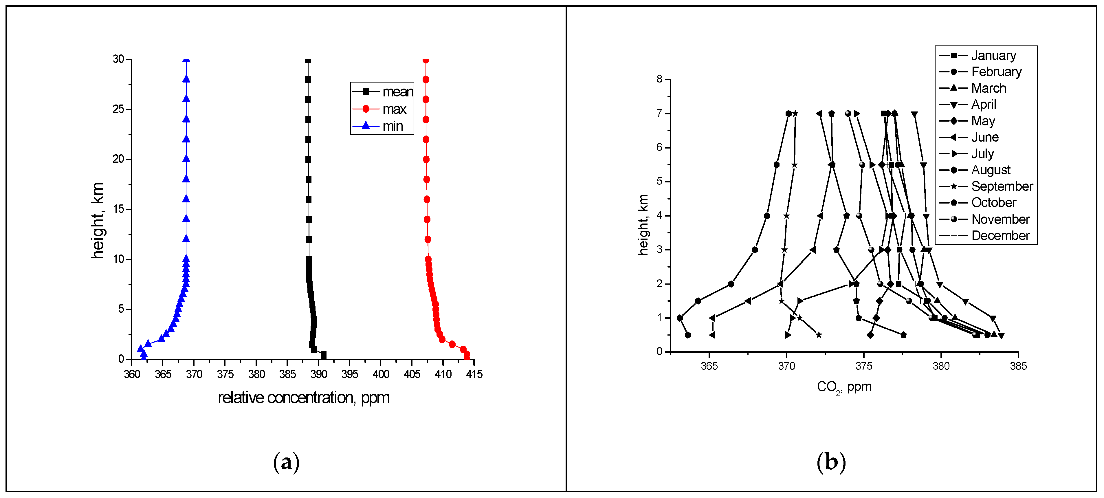
The standard IAO model [42] was employed for other gases. The Krekov–Rakhimov model [43] was used as an optical aerosol model. The near-surface relative concentration of CO2 varies from 360 to 415 ppm, with regard for the growth of the carbon dioxide concentration in the last decade (Figure 1). For example, in [7], the value of 410 ppm was taken for the estimation of the lidar capabilities. As the vertical concentration profiles of CO2 in the troposphere, we take the results of monthly observations in Western Siberia by IAO SB RAS (Institute of atmospheric optics Russian Academy of Science, Siberian branch) aircraft An2-30 Optic [38,39]. The greatest fluctuations in the concentration of carbon dioxide are observed at altitudes of 0.5–2 km [38,39].
We use the direct simulation, that is, normal noise corresponding to the signal-to-noise ratio with regard for the shot and thermal noise is superimposed onto every signal, and then the inverse problem is solved [13].
Subsequently, the learning of neural networks is performed with signals at different atmospheric situations as examples. In addition, the algorithm of pre-learning that is based on pseudo-inverse matrices (as developed by us) and the backpropagation algorithm are invoked. When assessing the possibilities of retrieval, the data on reflected signals, data on scattered DIAL signals, and the pressure and temperature profiles (that is, the most complete set of available a priori data) are considered as input data for the network.
When learning examples are formed, it is desirable to perform pre-normalization with allowance for some shift (10%) from the minimal and maximal values [13]:
where - unnormalized -th input or output value of -th learning sample.
For the learning, we took 5000 training examples and 5000 test examples. With fewer learning examples in the sample, the standard deviation of the error for different training samples is more than 0.1 ppm. The test examples were separately formed from the learning sample and not included in it. In addition, the cross-test sample of 500 examples was used. This sample serves for testing the network operation in the process of learning. The coefficients of the neural network, at which the network provides the smallest average error, both for the cross-test sample and for the learning sample, are taken. It should be noted that the formation of learning examples takes up to three days at a 2.4-MHz processor, with an allowance for the readout of data on the pressure, temperature, concentration of carbon dioxide, and other gases, as well as with calculations of the absorption coefficients with regard to the Voigt profile.
A three-layer neural network, with the number of neurons in the first layer being twice as large as the number of network inputs, is used. Reflected signals, refracted signals, pressure, and temperature up to 10 km with a step of 0.5 km serve as input data for the network. The data on the reflected signal are duplicated according to the amount of data regarding temperature and pressure if we use regularization when obtaining a pseudo-inverse matrix by adding a random uniform value with zero mean to the matrix of input values, and then do not duplicate when using the Tikhonov regularization method (although the results are not very different). Correspondingly, the number of inputs can reach 100 (up to 100 neurons in the first layer) and the number of neurons in the second layer is twice as large as that in the first one. The sigmoid function of neuron activation is used.
3. Results
The first experiment performed uses data on reflected, scattered signals, and all a priori data on the pressure profile and temperature profiles.
Table 2 provides the results for different high-altitude platforms at the effective reflection height of 50 m, pulse energy of 50 mJ,, and passband of 1 nm. The table presents data for the average weighted relative concentration . To calculate the standard deviation of the error, a statistical estimate was made and 20 training and test samples were created, on which the network was trained and the error was calculated for each of the neural networks. As expected, the error when probing from lower heights falls. At the same time, when probing from altitudes of 10 km, a decrease in the error also occurs, due to the use of a back-scattered signal.
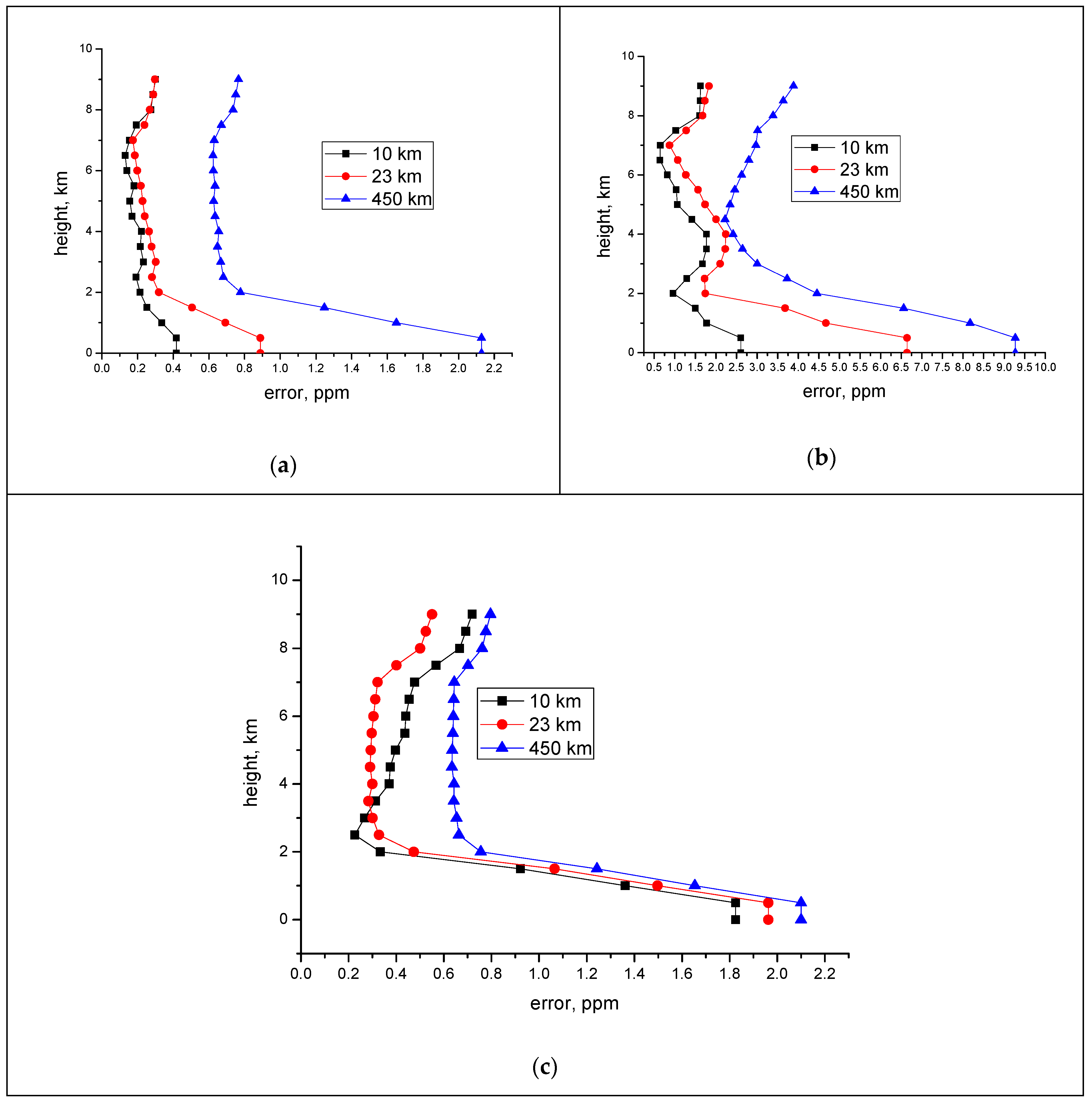
Figure 2 shows the average and the maximal errors of retrieval of the relative concentration at the different heights that the platform with the installed lidar is located at. The results of carbon dioxide concentration errors were obtained for the case of using data on the profile of temperature, pressure, and the back scattered and reflected signal.
If the average error is reconstructed with an acceptable accuracy, then the error of retrieval of the relative concentration at the given height is far larger, especially at low heights.
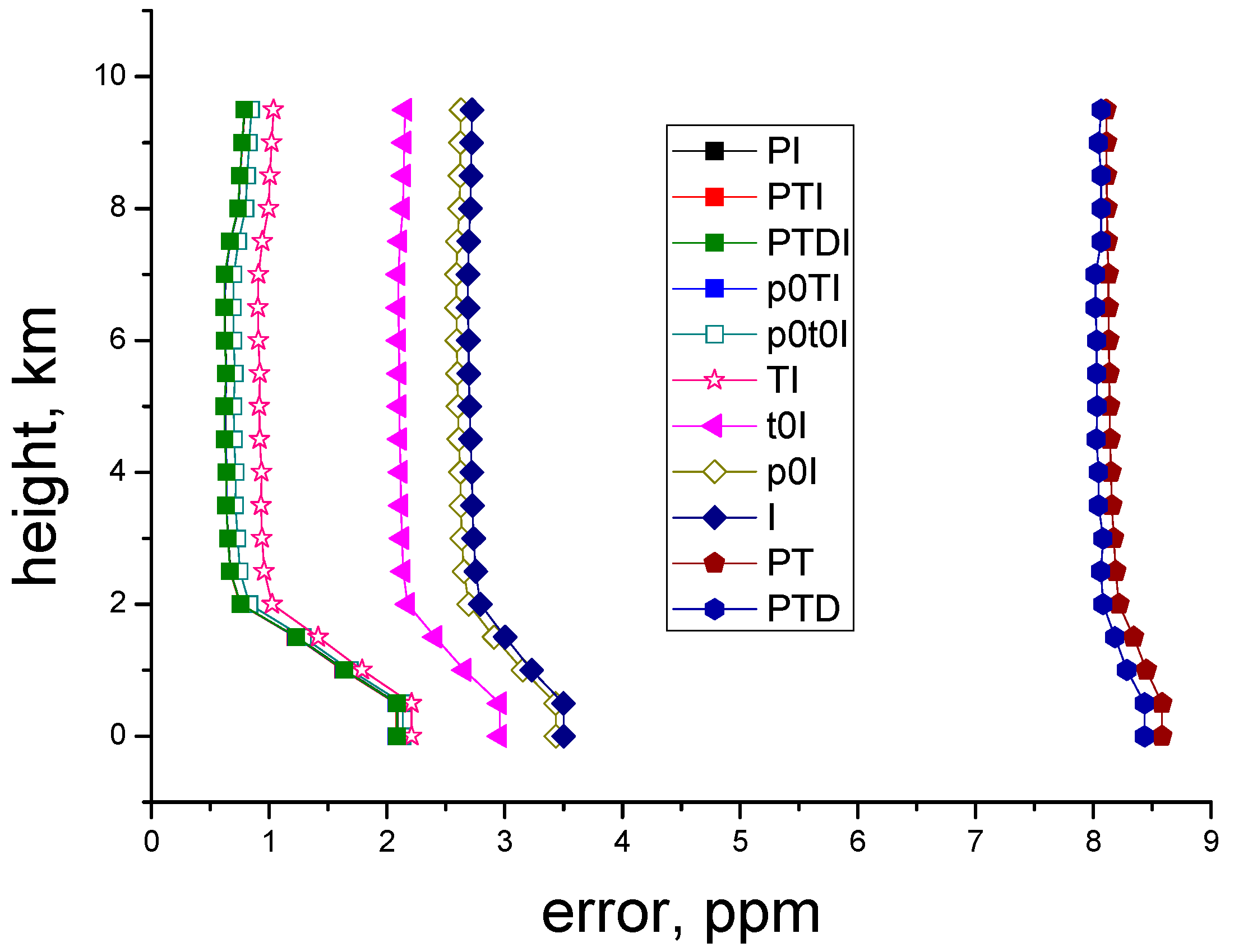
For the next experiments, we have chosen several variants of the types of input data and their combinations. The temperature profile, pressure profile, profile of the ratio of on and off scattered signals (DIAL), and profile of the ratio of two reflected signals (IPDA) serve as the main combined parameters. These combinations are presented below. Here, n means that the n data for heights are taken. If 0, then one value is taken, for temperature, this value is taken near the Earth’s surface.
- Pressure (n) + IPDA.
- Pressure (n) + Temperature (n) + IPDA.
- Pressure (n) + Temperature (n) + DIAL (n) + IPDA.
- Pressure (0) + temperature (n) + IPDA.
- Pressure (0) + Temperature (0) + IPDA.
- Temperature (n) + IPDA.
- Temperature (0) + IPDA.
- Pressure (0) + IPDA.
- IPDA.
- Pressure (n) + Temperature (n)
- Pressure (n) + Temperature (n) + DIAL (n)
Figure 3 depicts the errors of operation of the neural network as functions of the used set of initial data. It is obvious that the best results are obtained for the first situation, when both the IPDA and the DIAL signals are used, as well as the data on the pressure and temperature at all heights, that is, at the use of all a priori data. The errors in the cases where the profiles of temperature and pressure are used and the errors in the cases where only the pressure at the surface level and the temperature profile are used, as well as in the cases of only the pressure profile, practically coincide (approximately, 2.15 ppm on the surface). A little bit worse results (2.3 ppm on the surface) are obtained for the case where only the temperature profile and the signals are used. The worst results are obtained for the case when only the IPDA signal or the IPDA signal along with the DIAL signal is used. The worst case is the use of only the DIAL signal, even if together with the temperature and pressure profiles, when the error of the near-surface relative concentration is 7 ppm. Thus, the use of the DIAL signal at the sensing from a spacecraft makes no sense.
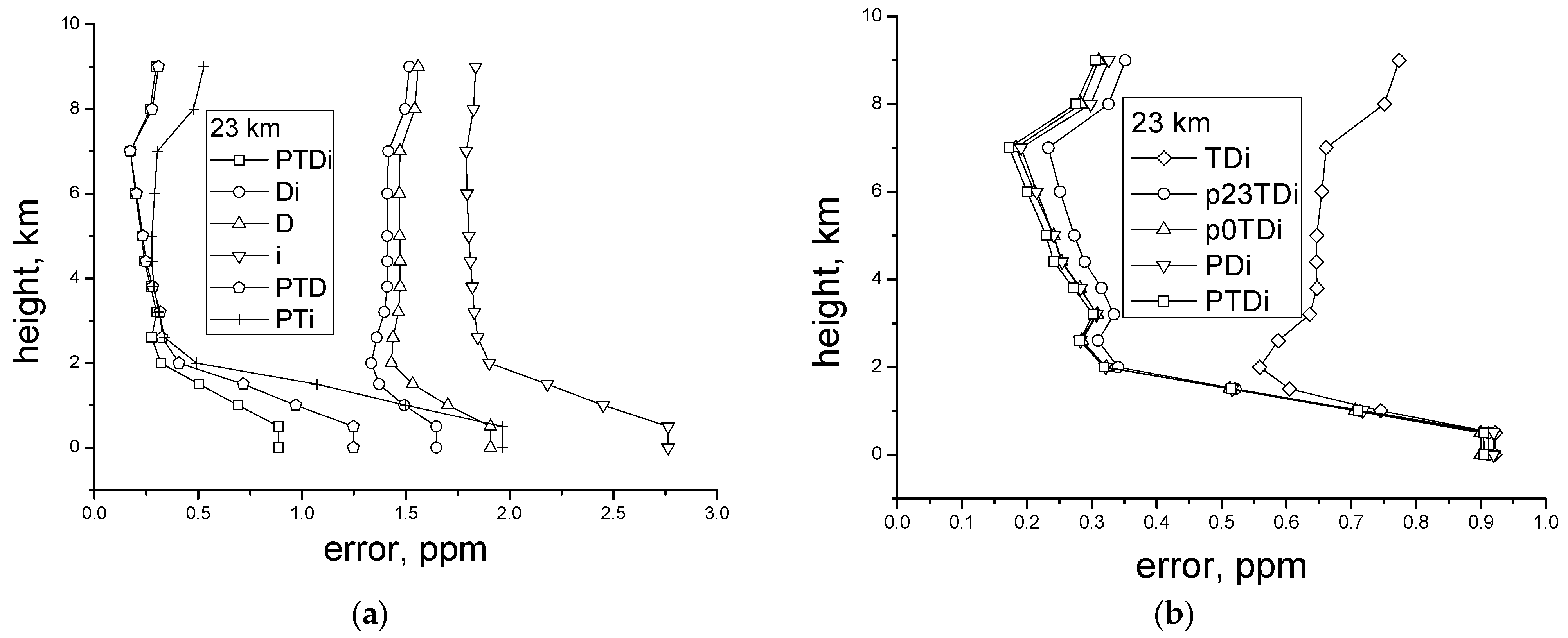
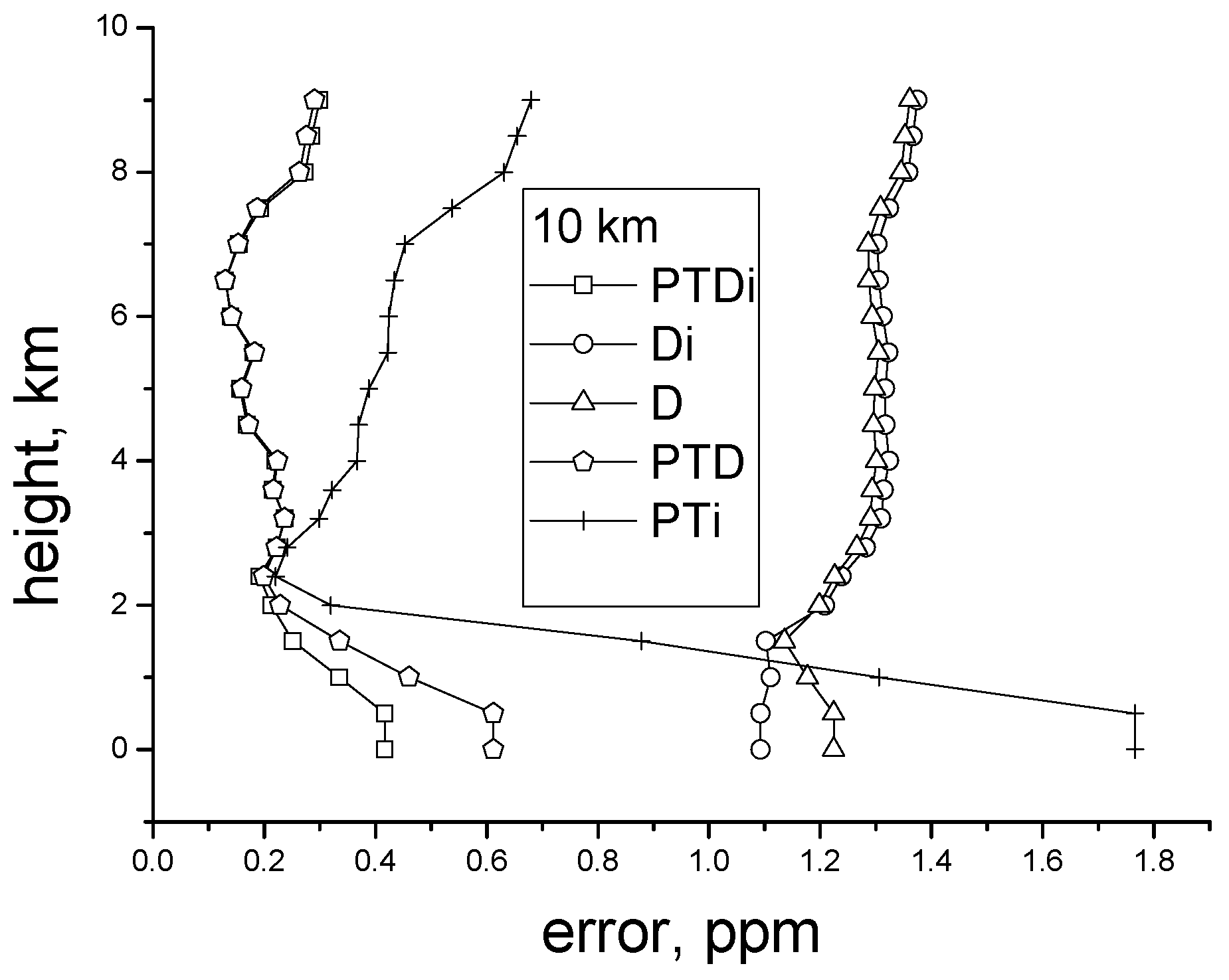
Below, we consider the possibilities of the neural network for the retrieval of the profiles of relative carbon dioxide concentration at the lidar height of 23 km and 10 km (Figure 4a,b). Here, for comparison, we use the examples in which the laser pulse energy is 100 mJ, that is, twice as high as in the previous examples. This test demonstrates at which characteristics the error that is smaller than 1 ppm can be attained at near-surface heights in the case of sensing from 23 and 10 km. The sensing from a 23-km platform assumes the use of a stratospheric aerostat, while for the sensing from 10 km, an aerostat or aircraft can be used.
Thus, the best results were obtained for the situation that all a priori data are known. In this case, the average achievable error at the near-surface heights is smaller than 1 ppm–0.8 ppm. The worst results are attained when the data only on the DIAL or IPDA signals are used. The combination of both the DIAL and IPDA signals provides an improvement in accuracy. In this case, the DIAL signals give the higher accuracy in comparison with the IPDA signals, both with and without the use of the pressure and temperature profiles. It should be noted that the laser pulse duration is taken to be 30 ns. Therefore, in this case, the DIAL signal provides a weighty contribution to the possibility of retrieval of the concentration profile. In total, the knowledge regarding a priori data on the pressure and temperature profiles improves the possibility of retrieval by 1–1.5 ppm in accuracy when compared to the case when these data are unknown. At the same time, the knowledge of only the IPDA signal or only the DIAL signal does not allow for the concentration at the near-surface heights to be retrieved with an error that is smaller than 1 ppm. This retrieval is only possible with the joint use of DIAL and IPDA at the known pressure and temperature profiles. At heights above 2 km with the known pressure and temperature profiles, the errors are practically identical in the cases when the signals of different types are used separately or together. With the use of only the temperature profile, the error is higher (Figure 4b). The use of the pressure at a height of 23 km gives a slightly larger error than the use of the entire pressure profile and the temperature or the pressure at a height of 0 km.
The same conclusions are true for the sensing from a height of 10 km, but only the error is more than halved in comparison with the sensing from 23 km (Figure 5). Thus, for such systems, the technical requirements can be decreased more than twice.
It should be noted that, when only the reflected signal is used, the retrieval of the profile is characterized by the much higher error than the retrieval of the average concentration. In addition, generally, the vertical profile of the concentration significantly affects the error of retrieval of the vertical profile and, thus, the accuracy of retrieval of the near-surface concentration, but its effect on the error of retrieval of the average concentration is less significant.
4. Discussion
The obtained results show the possibility of application of neural networks in the problem of estimating both the concentration profile of carbon dioxide and mean concentration, as well as the possibility of simultaneously estimating both the profile and the mean concentration was investigated. This technology allows for use of supplementary data, including the profile of pressure and temperature. As expected, in accordance with the barometric height formula, it is sufficient to use either a pressure profile or a temperature profile and pressure value at a certain altitude point, in which case the determination errors are almost identical.
Obviously, invoking a priori data on the pressure profile leads to a considerable increase in the accuracy of retrieval. The data on temperature also give higher accuracy, but only by 0.2–0.4 ppm. If the data regarding the temperature profile are combined with the data on the near-surface pressure, then the error is comparable with that at the known entire pressure profile and temperature. At the sensing from heights of 23 and 10 km, the joint use of DIAL and IPDA signals provides better results in accuracy than the separate use of DIAL or IPDA signals. The use of DIAL signals is impractical at the sensing from onboard a spacecraft.
For more accurate measurements, it is essential to know the pressure profile or the temperature profile with the pressure being known at some near-surface height.
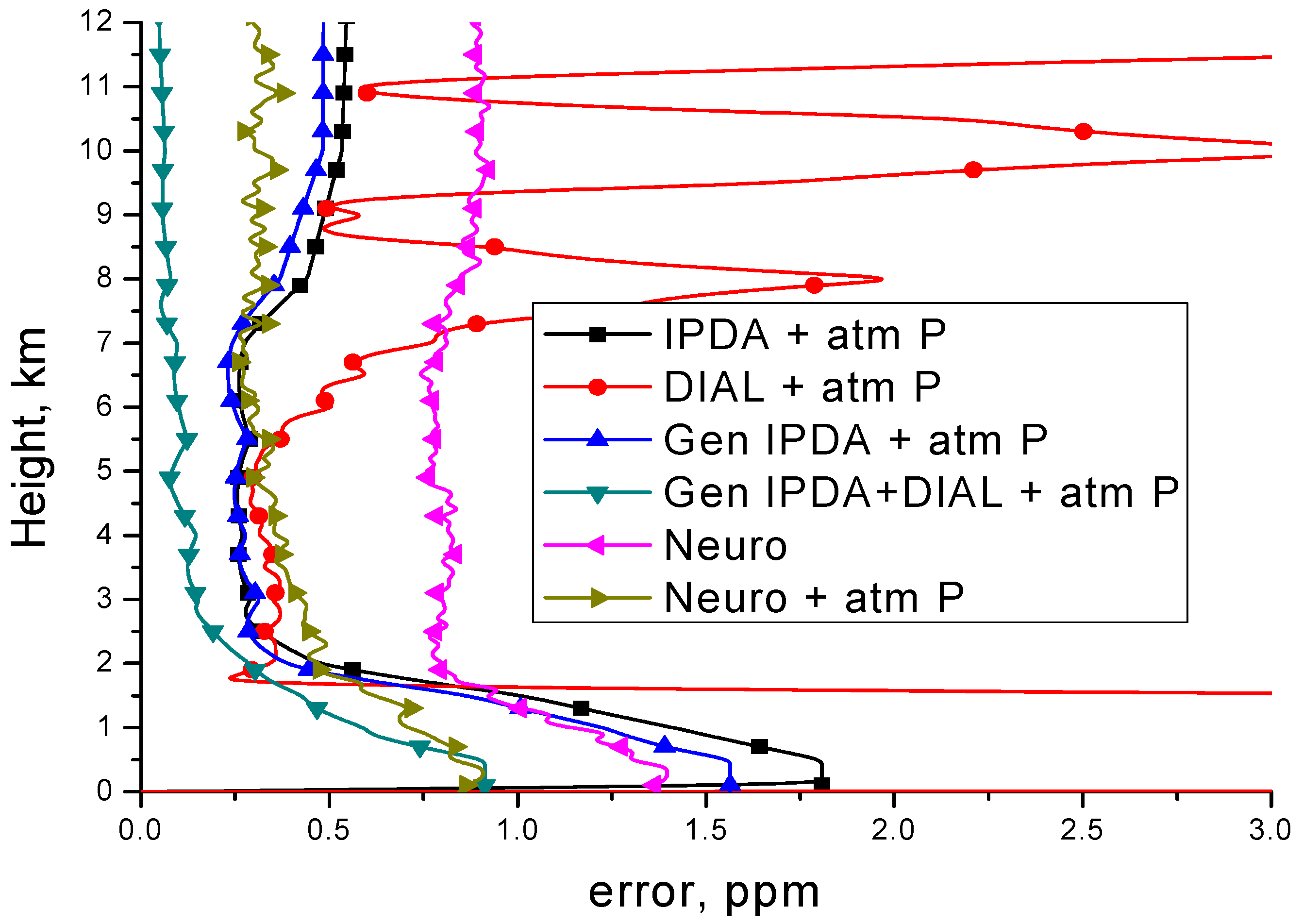
Part of our research has already been devoted to the study of the use of lidars for probing carbon dioxide, both from the side of the space platform and the balloon. For example, in [9], it was shown that the differential signal processing scheme on and off neutralizes the effect of multiple scattering. Multiple scattering slightly influences the signal power, even in the presence of fogs and clouds when the lidar is in high orbit. Besides, we considered the possibility of using not only direct detection, but also heterodyne detectors [44]. Our further research is aimed at the use of modulated laser emission, and taking into account the height of the surface above the territory of Siberia and Russia, to compile a map of measurement errors of both the mean and near-surface concentrations, and to develop search algorithms for sources of greenhouse gases, including methane. As methods, we are using machine learning and computational intelligence approaches, such as neural networks and genetic algorithms. For these problems, they allow for improving estimation capabilities in noise conditions and systematic errors. For example, comparing standard resolving approaches and computational intelligence methods was carried out in [13]; the application of computational intelligence algorithms increased the retrieval possibility of carbon dioxide concentration profile (Figure 6).
It shows how, when sounding from a height of 23 km, even while using a known profile, it is difficult to use standard approaches to estimate the concentration profile. Even the preliminary smoothing of the DIAL signal results in significant errors at the boundaries of height intervals, and the use of an IPDA signal using a set of base altitude vectors still provides a large error. Work [13] allowed for us to draw a conclusion regarding the significant effect of the profile’s altitude profile on the error of estimation the near-surface concentration. In general, the use of neural networks is limited by the possible difficulties in creating training samples, respectively, the adequate modeling of signals, and creating a data bank of atmospheric situations. To avoid binding to the signal power, the input of the neural network was given the ratio of signals on and off.
5. Conclusions
Our studies demonstrate the possibility of lidar application in the sensing of carbon dioxide from onboard a spacecraft orbiting at a height of 450 km, with an error of retrieval of the average relative concentration of 0.65 ppm or 0.15–0.16% (which is twice as high as the OСO-2 capabilities) up to 10 km at the laser pulse energy of 50 mJ, the receiving mirror 1 m in diameter, and 400 accumulated pulses, corresponding to the resolution of 60 km at the spacecraft velocity of 7.5 km/s. The error of the relative concentration at heights up to 2 km is 2 ppm, which imposes more rigorous requirements on the technical characteristics of a lidar for achieving higher accuracy at these heights.
The capabilities in the accuracy of retrieval of the average concentration at the sensing from heights of 23 km and 10 km with the same technical characteristics are two and three times higher, respectively.
The application of neural networks in the retrieval of the concentration allows for us to use additional a priori information and relate various input and output data.
Author Contributions
G.GM. was responsible for the statement of the problem, the results discussion, the conceptualization. A.Y.S. was responsible for developing methods and algorithms, setting up a numerical experiment, numerical modeling, solving an inverse problem, programming and analyzing results.
Funding
This research received no external funding.
Acknowledgments
This work was supported by the federal target program “Research and development in priority areas of development of the Russian scientific and technological complex for 2014-2020”.
Conflicts of Interest
The authors declare no conflict of interest.
References
- Ehret, G.; Kiemle, C.; Wirth, M.; Amediek, A. Space-borne remote sensing of CO2, CH4, and N2O by integrated path absorption lidar: A sensitivity analysis. J. Appl. Phys. 2008, 90, 593–608. [Google Scholar] [CrossRef]
- Mao, J.; Ramanathan, A.; Abshire, J.B.; Kawa, S.R.; Riris, H.; Allan, G.R.; Rodriguez, M.; Hasselbrack, W.E.; Sun, X.; Numata, K.; et al. Measurement of atmospheric CO2 column concentrations to cloud tops with a pulsed multi-wavelength airborne lidar. Atmos. Meas. Tech. 2018, 11, 127–140. [Google Scholar] [CrossRef]
- Han, G.; Ma, X.; Liang, A.; Zhang, T.; Zhao, Y.; Zhang, M.; Gong, W. Performance Evaluation for China’s Planned CO2-IPDA. Remote Sens. 2017, 9, 768. [Google Scholar] [CrossRef] [Green Version]
- Ehret, G.; Bousquet, P.; Pierangelo, C.; Alpers, M.; Millet, B.; Abshire, J.B.; Bovensmann, H.; Burrows, J.P.; Chevallier, F.; Ciais, P.; et al. MERLIN: A French-German Space Lidar Mission Dedicated to Atmospheric Methane. Remote Sens. 2017, 9, 1052. [Google Scholar] [CrossRef] [Green Version]
- Sakaizawa, D.; Kawakami, S.; Nakajima, M.; Tanaka, T.; Morino, I.; Uchino, O. An airborne amplitude-modulated 1.57 μm differential laser absorption spectrometer: Simultaneous measurement of partial column-averaged dry air mixing ratio of CO2 and target range. Atmos. Meas. Tech. 2013, 6, 387–396. [Google Scholar] [CrossRef]
- Menzies, R.T.; Spiers, G.D.; Jacob, J. Airborne Laser Absorption Spectrometer Measurements of Atmospheric CO2 Column Mole Fractions: Source and Sink Detection and Environmental Impacts on Retrievals. J. Atmos. Ocean. Technol. 2014, 31, 404–421. [Google Scholar] [CrossRef]
- Kiemle, C.; Ehret, G.; Amediek, A.; Fix, A.; Quatrevalet, M.; Wirth, M. Potential of Spaceborne Lidar Measurements of Carbon Dioxide and Methane Emissions from Strong Point Sources. Remote Sens. 2017, 9, 1137. [Google Scholar] [CrossRef] [Green Version]
- Matvienko, G.G.; Krekov, G.M.; Sukhanov, A.Y. Space-borne remote sensing of greenhouse gases by IPDA lidar: A potentialities estimate. In Proceedings of the 25th International Laser Radar Conference, St. Petersburg, Russia, 5–9 July 2010. [Google Scholar]
- Babchenko, S.V.; Matvienko, G.G.; Sukhanov, A.Y. Assessing the possibilities of sensing CH4 and CO2 greenhouse gases above the underlying surface with satellite-based IPDA lidar. Atmos. Ocean. Opt. 2015, 28, 37–45. [Google Scholar] [CrossRef]
- Connor, B.; Bösch, H.; McDuffie, J.; Taylor, T.; Fu, D.; Frankenberg, C.; O’Dell, C.; Payne, V.H.; Gunson, M.; Pollock, R.; et al. Quantification of uncertainties in OCO-2 measurements of XCO2: Simulations and linear error analysis. Atmos. Meas. Tech. 2016, 9, 5227–5238. [Google Scholar] [CrossRef]
- Wunch, D.; Wennberg, P.O.; Osterman, G.; Fisher, B.; Naylor, B.; Roehl, C.M.; O’Dell, C.; Mandrake, L.; Viatte, C.; Kiel, M.; et al. Comparisons of the Orbiting Carbon Observatory-2 (OCO-2) XCO2 measurements with TCCON. Atmos. Meas. Tech. 2017, 10, 2209–2238. [Google Scholar] [CrossRef]
- Orbiting Carbon Observatory-2 (OCO-2). Home Page. Available online: https://ocov2.jpl.nasa.gov/mission/quickfacts/ (accessed on 30 September 2018).
- Sukhanov, A.Y. Airborne DIAL-IPDA lidar sensing of carbon dioxide inverse problem solution on basis bionic methods. Optika Atmosfery i Okeana 2017, 30, 589–597. (In Russian) [Google Scholar]
- Frate, F.D.; Schiavon, G. A combined natural orthogonal functions/neural network technique for radiometric estimations of atmospheric profiles. Radio Sci. 1998, 33, 405–410. [Google Scholar] [CrossRef]
- Frate, F.D.; Schiavon, G. Neural networks for retrieval of water vapor and liquid water from radiometric data. Radio Sci. 1998, 33, 1373–1386. [Google Scholar] [CrossRef]
- Frate, F.D.; Schiavon, G. Nonlinear principal component analysis for the radiometric inversion of atmospheric profiles by using neural networks. IEEE Trans. Geosci. Remote Sens. 1999, 37, 2335–2342. [Google Scholar] [CrossRef]
- Hadji-Lazaro, J.; Clerbaux, C.; Thria, S. Inversion algorithm using neural networks to retrieve atmospheric CO total columns from high-resolution nadir radiances. J. Geophys. Res. 1999, 104, 23841–23854. [Google Scholar] [CrossRef]
- Frate, F.D.; Casadio, S.; Zehner, C. Retrieval of ozone profiles by using GOME measurements and a neural network algorithm. In Proceedings of the IEEE 2000 International Geoscience and Remote Sensing Symposium. Taking the Pulse of the Planet: The Role of Remote Sensing in Managing the Environment, IGARSS’2000, Honolulu, HI, USA, 24–28 July 2000; pp. 250–253. [Google Scholar]
- Jimenez, C.; Eriksson, P. A neural network technique for inversion of atmospheric observation from microwave limb sounders. Radio Sci. 2001, 36, 941–945. [Google Scholar] [CrossRef]
- Jimenez, C.; Eriksson, P.; Askne, J. Non-linear inversion of Odin sub-mm observation in the lower stratosphere by neural networks. Radio Sci. 2000, 200, 503–514. [Google Scholar] [CrossRef]
- Aires, F.; Prigent, C. A new neural network approach including first guess for retrieval of atmospheric water vapor, cloud liquid water path, surface temperature, and emissivities over land from satellite microwave observations. J. Geophys. Res. 2001, 106, 14887–14907. [Google Scholar] [CrossRef] [Green Version]
- Aires, F. Neural network uncertainly assessment using Bayesian statistics with application to remote sensing: 1. Network weights. J. Geophys. Res. 2004, 109, D10303. [Google Scholar] [CrossRef]
- Aires, F. Neural network uncertainly assessment using Bayesian statistics with application to remote sensing: 2. Output errors. J. Geophys. Res. 2004, 109, D10303. [Google Scholar] [CrossRef]
- Sukhanov, A.Y. Algorithms, Methods, and Software for Solution of Problems of Lidar Sensing of the Atmosphere. Ph.D. Thesis, Tomsk State University of Control Systems and Radioelectronics, Engineering Sciences, Tomsk, Russia, 2006; 151p. (In Russian). [Google Scholar]
- Mamun, M.M.; Müller, D. Retrieval of Intensive Aerosol Microphysical Parameters from Multiwavelength Raman/HSRL Lidar: Feasibility Study with Artificial Neural Networks. Atmos. Meas. Tech. 2016, 46. [Google Scholar] [CrossRef]
- Berdnik, V.V.; Loiko, V.A. Neural networks for aerosol particles characterization. J. Quant. Spectrosc. Radiat. Transf. 2016, 184, 135–145. [Google Scholar] [CrossRef]
- Krekov, G.M.; Krekova, M.M.; Lisenko, A.A.; Sukhanov, A.Y. Identification of minor pathogenic admixtures in the atmosphere based on the method of artificial neural networks, Siberian Aerosols. In Proceedings of the 15th Workshop, Tomsk, Russia, 2008; p. 41. [Google Scholar]
- Sukhanov, A.Y. On the algorithm of pre-learning of a neural network as applied to some inverse problems of lidar sensing, Atmospheric and Ocean Optics. Atmospheric Physics. In Proceedings of the XXII International Symposium, Tomsk, Russia, 30 June–3 July 2016; IAO SB RAS: Tomsk, Russia, 2016; pp. C45–C48, ISBN 978-5-94458-159-4. [Google Scholar]
- Sukhanov, A.Y.; Krekov, G.M. Recognition of fluorescence spectra of bacteria and polyaromatic hydrocarbons. In Proceedings of the All-Russian Conference on Mathematical Methods of Image Recognition, Petrozavodsk, Russia, 11–17 September 2011; MAKS Press: Moscow, Russia, 2011; pp. 514–517. [Google Scholar]
- Kataev, M.Y.; Sukhanov, A.Y. Capabilities of the neural network method for retrieval of the ozone profile from lidar data. Atmos. Ocean. Opt. 2003, 16, 1020–1023. [Google Scholar]
- DeepLearning4j. Deep Learning for Java. Home Page. Available online: https://deeplearning4j.org/ (accessed on 20 September 2018).
- Keras: The Python Deep Learning library. Home Page. Available online: https://keras.io/ (accessed on 20 September 2018).
- Goodfellow, I.J.; Warde-Farley, D.; Lamblin, P.; Dumoulin, V.; Mirza, M.; Pascanu, R.; Bergstra, J.; Bastien, F.; Bengio, Y. Pylearn2: A machine learning research library. arXiv, 2013; arXiv:1308.4214. [Google Scholar]
- Tikhonov, A.N.; Arsenin, V.Y. Solution of Ill-Posed Problems; Winston & Sons: Washington, DC, USA, 1977; 258p, ISBN 0-470-99124-0. [Google Scholar]
- El’nikov, A.V.; Zuev, V.V.; Kataev, M.Y.; Marichev, V.N.; Mitsel, A.A. Sounding of stratospheric ozone with an UV bifrequency DIAL: Methods for solving the inverse problem and results of the field experiment. Atmos. Ocean. Opt. 1992, 5, 362–369. [Google Scholar]
- Galushkin, A.I. (Ed.) Neural Network Theory; Springer: Berlin, Germany, 2007; pp. 1–52. ISBN 978-3-540-48125-6. [Google Scholar]
- Holland, J.H. (Ed.) Adaptation in Natural and Artificial Systems; University of Michigan Press: Ann Arbor, MI, USA, 1975; 183p. [Google Scholar]
- Arshinov, M.Y.; Belan, B.D.; Davydov, D.K.; Krekov, G.M.; Fofonov, A.V.; Babchenko, S.V.; Inoue, G.; Machida, T.; Maksutov, S.; Sasakawa, M.; et al. The dynamics in vertical distribution of greenhouse gases in the atmosphere. Optika Atmosfery i Okeana. 2012, 25, 1051–1061. (In Russian) [Google Scholar]
- Arshinov, M.Y.; Belan, B.D.; Davydov, D.K.; Inouye, G.; Maksyutov, Sh.; Machida, T.; Fofonov, A.V. Vertical distribution of greenhouse gases above Western Siberia by the long-term measurement data. Atmos. Ocean. Opt. 2009, 22, 316–324. [Google Scholar] [CrossRef]
- Labitzke, K.; Barnett, J.J.; Edwards, B. Handbook MAP 16; Edwards, B., Ed.; University of Illinois: Urbana, IL, USA, 1985; 320p. [Google Scholar]
- Hedin, A.E. Extension of the MSIS Thermospheric Model into the Middle and Lower Atmosphere. J. Geophys. Res. 1991, 96, 1159–1172. [Google Scholar] [CrossRef]
- Komarov, V.S. (Ed.) Statistical Models of Temperature and Gaseous Constituents of the Atmosphere; Gidrometeoizdat: Leningrad, Russia, 1986; 264p. [Google Scholar]
- Balin, Y.S.; Borovoi, A.G.; Burlakov, V.D.; Dolgii, С.I.; Klemasheva, M.G.; Konoshonkin, A.V.; Kokhanenko, G.P.; Kustova, N.V.; Marichev, V.N.; Matvienko, G.G.; Nevzorov, A.A.; Nevzorov, A.V.; et al. Lidar Monitoring of Cloud and Aerosol Fields, Minor. Gaseous Constituents, and Meteorological Parameters of the Atmosphere; Matvienko, G.G., Ed.; IAO SB RAS: Tomsk, Russia, 2015; 450p, ISBN 978-5-94458-156-3. [Google Scholar]
- Matvienko, G.G.; Sukhanov, A.Y. Space-borne remote sensing of CO2 by IPDA lidar with heterodyne detection: Random error estimation. Proc. SPIE 2015, 9680, 96804I. [Google Scholar]
Figure 1.
Range of variability of the relative concentration for creation of examples of the learning and test samples. (a). Example of monthly averaged data for multiyear measurements of carbon dioxide concentration profiles from 1997 to 2008 over western Siberia (b).
Figure 1.
Range of variability of the relative concentration for creation of examples of the learning and test samples. (a). Example of monthly averaged data for multiyear measurements of carbon dioxide concentration profiles from 1997 to 2008 over western Siberia (b).

Figure 2.
Average (a) and maximal (b) errors of retrieval of the relative concentration at the given height (Neural Network method). Standard IPDA method error (c).
Figure 2.
Average (a) and maximal (b) errors of retrieval of the relative concentration at the given height (Neural Network method). Standard IPDA method error (c).

Figure 3.
Absolute average errors of retrieval of the profiles of relative carbon dioxide concentration at the sensing from the height of 450 km.
Figure 3.
Absolute average errors of retrieval of the profiles of relative carbon dioxide concentration at the sensing from the height of 450 km.

Figure 4.
Retrieval for different combinations of input data (P is for the pressure profile, T is for the temperature profile, D is for the profile of the ratio of DIAL signals, and i is for the ratio of IPDA signals) (a), and errors of retrieval with the use of combinations of the pressure and temperature profiles (b).

Figure 5.
Error of sensing from a height of 10 km.

Figure 6.
Comparison of inverse tasks resolving algorithms based on the use of neural networks (Neuro), genetic algorithms (Gen), and the standard approach (IPDA, DIAL with using pressure profile atmP).
Figure 6.
Comparison of inverse tasks resolving algorithms based on the use of neural networks (Neuro), genetic algorithms (Gen), and the standard approach (IPDA, DIAL with using pressure profile atmP).


Table 1.
Parameters of the Lidar System.
| Parameter | Value |
|---|---|
| M, detector amplification coefficient | 20 |
| Q, quantum efficiency | 0.8 |
| B, passband, MHz | 3 |
| detector sensitivity | 1.012 |
| , laser pulse duration, ns | 30 |
| Pulse energy, J | 0.05, 0.1 |
| Divergence angle of laser radiation, mrad | 0.1 |
| Detector angle, mrad | 0.2 |
| F, excess noise factor | 4.3 |
| iD, dark current density, fA/Hz0.5 | 160 |
| i0, noise density of amplifier input current, fA/Hz0.5 | 4 |
| u0, voltage density of amplifier input current, nV/Hz0.5 | 3 |
| T, absolute temperature, K | 290 |
| RF, resistance, Mohm | 1 |
| Cdet, equivalent capacity of the detector system, pF | 4 |
| , height, km | 10, 23, 450 |
| Radius of receiving telescope, m | 0.5 |
| Number of accumulated pulses | 400 |
| Filter width, nm | 1 |
| , reflection coefficient, sr−1 | 0.08 |
| Energy brightness of solar radiation, mW/m2/nm | 5-day, 5 × 10⁻⁴-night |
Table 2.
Results of Numerical Experiment on Retrieval of the Relative CO2 Column Concentration (Pulse Energy of 50 mJ, 400 Pulses).
Table 2.
Results of Numerical Experiment on Retrieval of the Relative CO2 Column Concentration (Pulse Energy of 50 mJ, 400 Pulses).
| Platform Height | Weighted Average Error, ppm | Standard Deviation of Error, ppm | Weighted Maximal Error, ppm | Standard IPDA Method Error, ppm |
|---|---|---|---|---|
| 450 km | 0.64 | 0.09 | 3 | 0.67 |
| 23 km | 0.31 | 0.06 | 1.5 | 0.35 |
| 10 km | 0.125 | 0.02 | 1.0 | 0.21 |
© 2019 by the authors. Licensee MDPI, Basel, Switzerland. This article is an open access article distributed under the terms and conditions of the Creative Commons Attribution (CC BY) license (http://creativecommons.org/licenses/by/4.0/).
Share and Cite
MDPI and ACS Style
Matvienko, G.G.; Sukhanov, A.Y. Application of Neural Networks for Retrieval of the CO2 Concentration at Aerospace Sensing by IPDA-DIAL lidar. Remote Sens. 2019, 11, 659. https://0-doi-org.brum.beds.ac.uk/10.3390/rs11060659
AMA Style
Matvienko GG, Sukhanov AY. Application of Neural Networks for Retrieval of the CO2 Concentration at Aerospace Sensing by IPDA-DIAL lidar. Remote Sensing. 2019; 11(6):659. https://0-doi-org.brum.beds.ac.uk/10.3390/rs11060659
Chicago/Turabian StyleMatvienko, Gennadii G, and Alexander Ya Sukhanov. 2019. "Application of Neural Networks for Retrieval of the CO2 Concentration at Aerospace Sensing by IPDA-DIAL lidar" Remote Sensing 11, no. 6: 659. https://0-doi-org.brum.beds.ac.uk/10.3390/rs11060659
Note that from the first issue of 2016, this journal uses article numbers instead of page numbers. See further details here.