Inundation Extent Mapping by Synthetic Aperture Radar: A Review

Abstract

Recent flood events have demonstrated a demand for satellite-based inundation mapping in near real-time (NRT). Simulating and forecasting flood extent is essential for risk mitigation. While numerical models are designed to provide such information, they usually lack reference at fine spatiotemporal resolution. Remote sensing techniques are expected to fill this void. Unlike optical sensors, synthetic aperture radar (SAR) provides valid measurements through cloud cover with high resolution and increasing sampling frequency from multiple missions. This study reviews theories and algorithms of flood inundation mapping using SAR data, together with a discussion of their strengths and limitations, focusing on the level of automation, robustness, and accuracy. We find that the automation and robustness of non-obstructed inundation mapping have been achieved in this era of big earth observation (EO) data with acceptable accuracy. They are not yet satisfactory, however, for the detection of beneath-vegetation flood mapping using L-band or multi-polarized (dual or fully) SAR data or for urban flood detection using fine-resolution SAR and ancillary building and topographic data.

1. Introduction

Near-real-time (NRT) inundation extent mapping during flood events using remote sensing data is vital to support rescue and damage recovery decisions and to facilitate rapid assessment of property loss and damage. It also provides a two-dimensional reference for validating and calibrating real-time numerical modeling, including flood risk analysis at a regional to global scale [1,2,3]; flood event prediction at a small scale [4,5,6,7]; and the tradeoff evaluation between the accuracy and complexity of hydrodynamic simulation [8,9,10,11]. It is, moreover, a validation source for geomorphological analysis of flood vulnerability [12,13,14,15,16]. Retrieved inundation extent can also be converted to inundation depth [17,18,19,20].

Both optical sensors and passive and active microwave sensors can be used for inundation mapping, offering different levels of capacity, accuracy, and solution difficulty. By means of water indices, optical remote sensing data can be used to extract water surfaces straightforwardly and reliably. As long-term, fine-resolution satellite data (such as Landsat data) are accumulated and new satellites (such as Sentinel-2) are started to serve, optical remote sensing methods are contributing significantly to the delineation of global and regional water surfaces [21,22,23,24]. The validity of optical observations is limited, however, by clouds and unclear weather conditions, which are common during flood events.

Microwave remote sensing techniques, on the other hand, have good penetration through the atmosphere and therefore can provide more efficient measurement. Pixel water fraction estimated from passive microwave measurement—the brightness temperature—features low spatial (~25 km, ¼ degree) but fine temporal resolution (daily) [25,26]. The result is, therefore, usually downscaled up to 90 meters by topography [27] and/or optical sensor-derived water probability [28]. Such downscaling mechanisms may be valid for fluvial inundation at global and regional scale but can be problematic for small pluvial flooding at local scale.

By detecting the scattering mechanism, synthetic aperture radar (SAR) can be used to map inundation under almost any weather condition at fine to very fine spatial resolution (from 30 m to <1 m). As an active sensor, SAR works nocturnally as well. The retrieval algorithms using SAR data are more difficult to design than the sensors discussed above, and purely automated algorithms that require zero human interference are so far rare. With the growing availability of remote sensing data and the development of retrieval techniques, the automation and reliability of SAR data are expected to emerge soon.

This study focuses on evaluating existing inundation mapping algorithms, using SAR data developed from 1980 to the present. Given that the data, study areas, and validation methods vary among studies, we primarily evaluate algorithms, along with some recently emergent approaches, according to four criteria: automation, robustness, applicability, and accuracy.

2. Techniques to Produce SAR Inundation Maps

2.1. Principles

Change in surface roughness is the key to detecting inundation using SAR data. Where the ground surface is covered with water, its low roughness exhibits almost ideal reflective scattering, in strong contrast to the scattering of natural surfaces in dry conditions. Consequently, different scattering mechanisms can cause two opposing changes in the total backscattering intensity: dampening and enhancement.

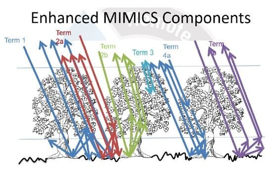
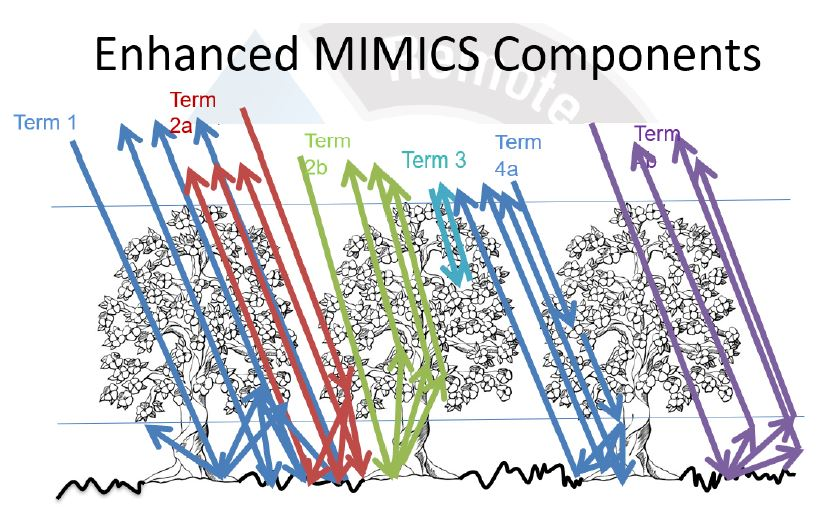
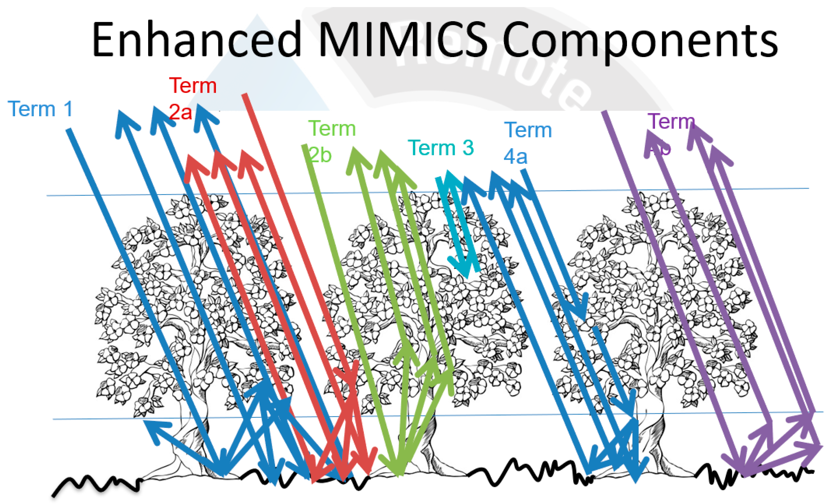
In the case of an open flood where water is not obscured by vegetation or buildings, dampening occurs because most of the scattering intensity is concentrated in the forward direction, whereas the back direction is very weak. In vegetated areas, different scattering mechanisms can happen, depending on the vegetation structure and submerge status. In fully submerged locations, scattering dampening occurs as in an open flood, while scattering enhancement is observed in partially or unsubmerged locations because the dihedral scattering dominates. The backscattering components of vegetation (with a canopy layer) are derived in the enhanced Michigan microwave canopy scattering (enhanced MIMICS) model by Shen et al. [29] from the first-order approximation of the vectorized radiative transfer (VRT) equation [30,31].

As shown in Figure 1, the vegetation-ground system can be conceptualized by three layers from top to bottom: the canopy layer (C), the trunk layer (T), and the rough ground surface (G). Term 1 (G-C-G) in the figure, for instance, refers to the wave scattered by the ground surface after it penetrates the canopy, which is then scattered by the canopy back to the ground and is finally scattered back to the sensor after penetrating the canopy. Term 7 (direct scattering) indicates that the scattering process on the ground surface only occurs once between the two penetrations of the canopy.

A trunk is usually modeled by a cylindrical structure whose length is much greater than its diameter. Term 4a (T-G-C) in Figure 1 represents the scattering wave that consecutively penetrates the canopy layer first, is scattered forward by the trunk, is scattered back in the antenna’s direction, and, finally, penetrates the trunk and canopy layer. Term 4b (C-G-T) represents the scattering wave in the reverse order; under physical optical approximation, its forward scattering (in all azimuth directions) dominates. As a result, in 4a and 4b, only the forward scattering from the trunk is retained. If G is rough, the ground scattering energy is distributed to the upper hemisphere, and the forward direction is not very strong. When flooded, the ground surface is close to ideally smooth, and the forward scattering is significantly enhanced, which, in turn, significantly enhances 4a and 4b.

Another principle is to utilize interferometric SAR (InSAR) formed from repeated passes to detect non-obstructed flooded areas by identifying the loss of coherence over water surfaces [32,33,34,35]. However, coherence may only be used as the primary indicator where the background exhibits strong coherence, such as in highly developed urban areas whereas can only be used as a complementary source because the surface of a water body is not the only kind of area that loses coherence—the background is full of low-coherence areas, such as vegetation, shadow [36]. Similarly, utilizing differential InSAR (DInSAR) pairs from repeated tracks to detect inundation depth may only be feasible over background areas of strong coherence, which is not the case of beneath-vegetated inundation or non-obstructed inundation in natural areas.

Both non-obstructed flood and beneath-vegetation inundation can occur in natural areas; in urban areas, both non-obstructed-flood dampening effects and L-shaped-caused enhancement can be observed. A horizontal smooth inundated surface together with a vertical building can form an L-shaped corner reflector [37], which can be a strong scatterer when illuminated by the radar antenna. In addition, more areas can be shadowed by buildings than by natural terrain, resulting in greater uncertainty about flood detection in urban areas.

2.2. Error Sources

We attribute commonly seen errors to three sources: water-like surfaces, noise-like speckle, and geometric correction.

Water is not the only surface that exhibits close-to-specular scattering. Smooth surfaces at the scale of the measuring wavelength and shadowed areas share almost identical scattering properties with water surfaces; we refer to them hereafter as water-like surfaces. Water-like surfaces vary slightly with frequency and flood mapping algorithms. With sufficiently little roughness relative to wavelength, even bare soil can be misidentified as water. In procedures to detect non-obstructed water, water-like surfaces can create “false positives” or “over-detection.”

Noise-like speckle is encountered for almost all SAR applications and, in many, is considered a major disadvantage of SAR images over optical images. For example, unlike optical images, noncommercial SAR images with 5–10 m resolution, may not be suitable for detecting headwater flood. Since the floodplain of headwater may be only one or a few pixels wide, the water pixels can be contaminated severely by speckle and surrounding strong scatterers. Speckle is not real noise. The formation of speckle was well explained by Lee and Pottier [38] (p. 101): As “the distances between the elementary scatterers and the radar receiver vary due to the random location of scatterers, the received waves from each scatterer, although coherent in frequency, are no longer coherent in phase. A strong signal is received if wavelets are added relatively constructively, while a weak signal is received if the waves are out of phase.” As a result, homogeneous and continuous areas exhibit strong inhomogeneity in SAR images. As the sample number decreases with the improvement of spatial resolution, the backscattering of a pixel may not, be represented well by a known fully developed speckle model which increases the difficulty in classification. Although many SAR filtering techniques are developed, most of them reduces noise at the price of damaging image details, which can also propagate to inundation mapping. Modern techniques such as the selection of the optimal filter [39] and machine learning may offer some advanced way in suppressing speckle.

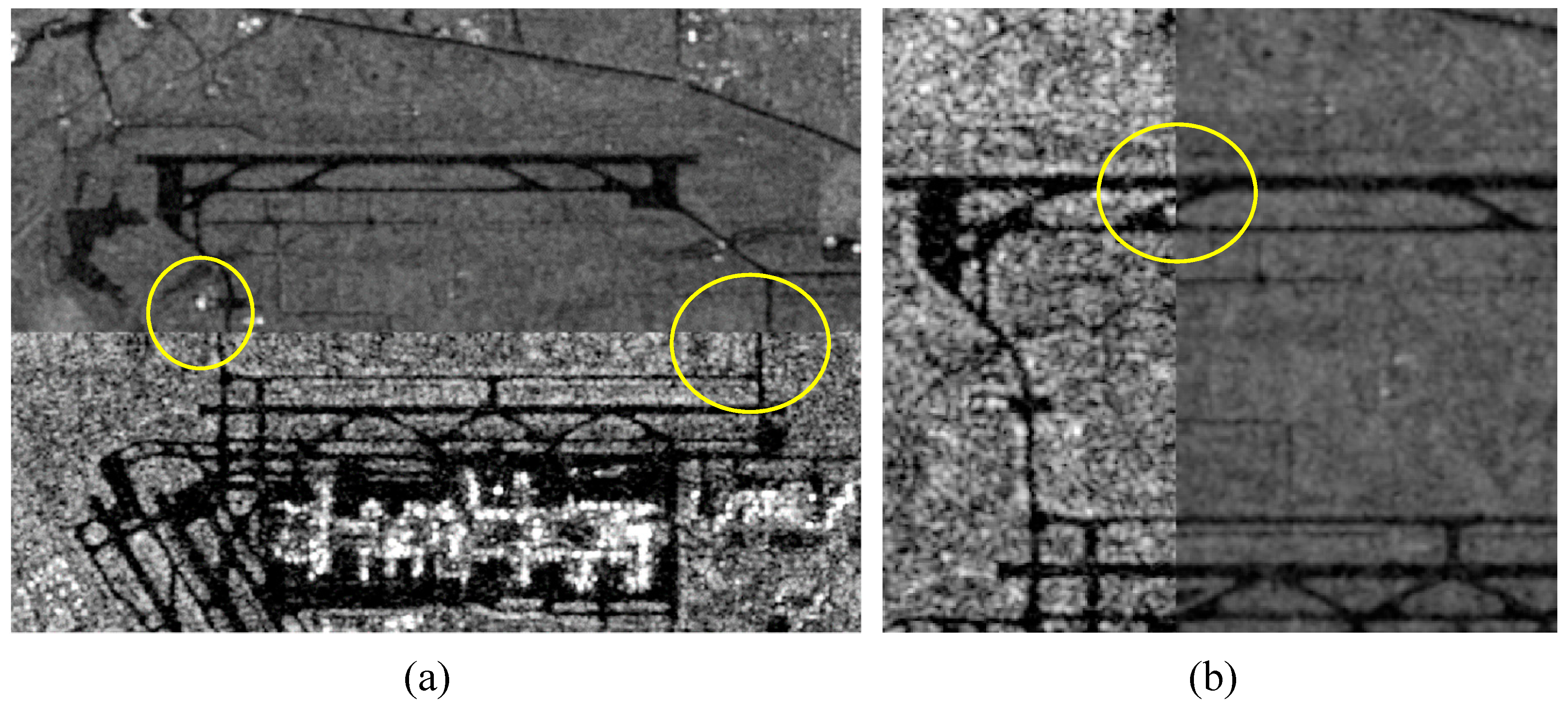
The original geometry of SAR images is range-azimuth. To be georeferenced, SAR images are often corrected to ground distance before high-level products are generated. Limited by the accuracy of input elevation data, the geometric correction algorithm, and orbit accuracy, it is common to see location errors at the level of a few pixels, as demonstrated in Figure 2. The offset in 10-pixel order in Figure 2 reflects the cumulatively geometric error of using Sentinel-1 images from different orbits, which can be significantly reduced using image pairs from the same orbit.

3. Relative Strengths and Limitations of Existing Techniques

3.1. Approaches

SAR-based inundation mapping methods are usually more complex than those based on optical sensors because of the processes added to mitigate the error propagated from one or more of the error sources mentioned above. Consequently, one study may consist of several different approaches introduced in the following.

3.1.1. Supervised Versus Unsupervised Methods

Mapping water extent is a matter of classification using supervised or unsupervised approaches. Supervised classification methods require a training set consisting of labeled inundated areas or core water locations and their corresponding pixels extracted from SAR data. Using training sets, mappers can achieve better accuracy without deeply understanding the physics of the data signal before designing an algorithm [40,41,42,43,44,45,46]. Drawbacks are at least twofold, however, the generation of training sets cannot be automated, and the algorithm has local dependence—that is, a classifier well-trained over one area may not work well in another.

Pulvirenti et al. [47] developed an “almost automatic” fuzzy logic classifier, which used fixed thresholds determined by a theoretical scattering model to classify pixels automatically or to use human-labeled samples. This method has proved reasonably accurate, but the automatic classification requires a microwave scattering model and introduces modeling uncertainty, while the human labeling of samples is time consuming. These drawbacks of supervised methods may be circumvented through the use of three unsupervised methods: threshold determination, segmentation, and change detection.

3.1.2. Threshold Determination

The specular reflective properties of non-obstructed water have driven many efforts [48,49,50,51] to determine a threshold below which pixels are identified as water. A single threshold may not hold well in large-area water bodies [52] or for the whole swath of a SAR image since it suffers from the heterogeneity of the environment, caused by wind-roughening and satellite system parameters [53]. Martinis and Rieke [54] demonstrated the temporal heterogeneity of the backscattering of permanent water bodies, implying the temporal variability of the threshold. To address the spatial variability, Martinis, Twele and Voigt [53] applied a split-based approach (SBA) [55], together with an object-oriented (OO) segmentation method [56]. Matgen et al. [51] introduced a histogram segmentation method, and Giustarini et al. [49] generalized the calibration process.

Essentially, a threshold-based approach needs to have either a bimodal image histogram (Figure 2 in Matgen, Hostache, Schumann, Pfister, Hoffmann and Savenije [51]) or some sample data to initialize the water distribution. To deal with non-bimodal histograms, manually drawing regions of interest (ROIs) is the most straightforward solution, but it impedes automation. For automation, SBA [53] ensures that only the splits showing a bimodal histogram (of water and non-water pixels) are used to derive a global threshold. On the other hand, Lu et al. [57] loosened the bimodal histogram restriction by initializing the water distribution using a “core flooding area” automatically derived from change detection, using multi-temporal SAR images. As change detection using only a single dry reference is sensitive to speckle and location error (see the subsection on change detection), the method may be affected. Furthermore, the threshold globalization of the method can be difficult.

More recently, dual-polarized (the common configuration of many active sensors) and fully polarized SAR data are utilized for threshold segmentation. After sampling pixels of high water probability from the global water occurrence map [58], and then removing out-of-bound samples by matching the peak, and 99% confidence interval of the sample histogram and the ${\chi }^2$ distribution, Shen et al. [59] automatically optimized the Wishart distribution and the probability density threshold of water in the dual-polarized domain. Since the water class is initialized before the threshold determination, this method is not restricted to bimodal histograms.

3.1.3. Segmentation

In contrast to pixel-based threshold determination, image segmentation techniques that group connected homogeneous pixels into patches can provide information at the object level—that is, at a higher level than the pixel—and are therefore believed to be more resistant to speckle because they utilize morphological information instead of radiometric information alone. The active contour method (ACM; [60,61]) allows a certain amount of backscattering heterogeneity within a water body and incorporates morphological metrics, such as curvature and tension. Martinis et al. [53] have applied OO segmentation [56] with SBA to reduce false alarms and speckle. Heremans et al. [62] compared the ACM and OO and concluded that the latter delineated the water areas more precisely than the former, which tend to overestimate their extension. Pulvirenti et al. [63] developed an image segmentation method consisting of dilution and erosion operators to remove isolated groups of water pixels and small holes in water bodies, which are believed to be caused by speckle. Giustarini et al. [49], Matgen et al. [51] and Lu et al. [57] employed the region growing algorithm (RGA) to extend inundation areas from detected water pixels. RGA starts from seeding pixels and then keeps absorbing homogenous pixels from neighbors until no more homogenous pixels exist in neighboring areas.

3.1.4. Change Detection

Change detection approaches traditionally refer to techniques for comparing pre- and in-flood backscattering intensities to detect changes in pixels caused by flooding [48,50,57,64,65]. One or more prior- and post-flood SAR image or images are needed; we refer to this hereafter as “dry reference.” The principle behind change detection techniques is straightforward, and the techniques should, theoretically, be effective in overcoming the first source of error—over-detection on water-like surfaces—as was shown by Giustarini et al. [49,51]. In the past, however, limited by their availability, change detection traditionally used only two SAR images. As a result, the aforementioned second-geometric error can only be avoided by limiting the using SAR images obtained from the same orbit or by indireclty evaluating the change from binary water mask; and the third error sources—speckle-caused noise—could compromise the effectiveness [66]. Shen et al. [59] have proposed an improved change detection (ICD) method that employs multiple (~5) pre-flood SAR images and a multi-criteria approach to reject false positives caused by water-like bodies and to reduce the effect of speckle.

More generally, change detection can be extended to the use of multiple dry references [59,67], the comparison of binary water maks [59], or InSAR coherence. The loss of InSAR coherence might be a more promising signature than the enhancement of intensity to detect buildings surrounded by inundation [33,34,35]. We refer to buildings surrounded by inundation as flooded buildings for simplicity, which should not be understood as flooded building floor or basement because satellite remote sensing images cannot detect the internal of buildings.

Besides isolating inundated areas from permanent (or, more precisely, preexisting) water areas, change detection techniques have been used to initialize water pixel sets before thorough detection [53,57], especially when full automation is an objective and no a priori water information is available. Change detection methods can also be used to detect flood beneath vegetation, as described in the next section.

3.1.5. Visual Inspection/Manual Editing Versus Automated Process

As discussed above, SAR-derived inundation results are affected by many error sources, which can hardly be eliminated by most algorithms. Visual inspection and manual editing could help in drawing training ROIs [42] and reducing false positives/negatives. As manual editing requires an overwhelmingly large workforce, it however, cannot be applied to rapid response to flood disasters, especially during back-to-back flood events. Studies aiming to improve automation include Pulvirenti et al. [47], Giustarini et al. [49], Matgen et al. [51], Martinis et al. [53], Horritt [60]; Horritt et al. [61], Pulvirenti et al. [63], Horritt et al. [68]; and Pulvirenti et al. [69].

3.1.6. Unobstructed, Beneath-Vegetation Flood Versus Urban Flood

Inundation detection over vegetated areas, partially submerged wetlands, and urban areas has gained attention recently. Theoretically, scattering is enhanced during flood time if a trunk structure exists. Ormsby et al. [70] evaluated the backscattering difference caused by flooding under canopy. Martinis and Rieke [54] analyzed the sensitivity of multi-temporal/multi-frequency SAR data to different land covers and concluded that X-band can only be used to detect inundation beneath sparse vegetation or forest during the leaf-off period, while L-band, though characterized by better penetration, has a very wide range of backscattering enhancement, which also obscures the reliability of the classification. Townsend [44] utilized ground data to train a decision tree to identify flooding beneath a forest using Radarsat-1 (http://www.asc-csa.gc.ca/eng/satellites/radarsat1/Default.asp). Horritt et al. [68] input the enhanced backscattering at C-band and phase difference of co-polarizations (HH-VV) to the ACM to generate water lines from selected known open water (ocean) and coastal dryland pixels. The area between the dry contour and open water was considered as flooded vegetation. Pulvirenti et al. [42] trained a set of rules using visually interpreted ROIs to extract flooded forest and urban areas from COSMO-SkyMed SAR data. Pulvirenti et al. [69] combined a fuzzy logic classifier [47] and segmentation method [63] to monitor flood evolution in vegetated areas using COSMO-SkyMed (http://www.e-geos.it/cosmo-skymed.html).

Given its potential for flood detection under vegetation, most studies have adopted a supervised classification, which can hardly be automated. Specifically, the enhanced dihedral scattering of vegetation cannot be considered as a single class because of different vegetation species, structure, and leaf-off and leaf-on conditions. Such heterogeneity makes it difficult to determine automatically a threshold of backscattering enhancement. In other words, the issue in detecting floods beneath vegetation is identifying multiple classes from an image, the automation of which is more challenging than identifying a single class.

Until now, few studies have been made available on flood mapping in urban areas [33,34,35,49,53,71,72], and only a handful [33,34,35,73] investigated the use of dihedral scattering to extract flooded buildings using either the intensity enhancement or the loss coherence. Because of the vertical structure of many buildings, the challenges in detecting urban inundation using intensity enhancement share some similarities with those of identifying floods under vegetation. An additional challenge arises from asymmetric building structure as compared to the symmetric structure of vegetation. Such enhancement only occurs when the radar line of sight (LoS) is orthogonal to the horizontal alignment of the building face [33,35]. Consequently, utilizing intensity enhancement cannot guarantee complete detection of flooded buildings and requires to know the geometry, orientation, and even material of buildings, and the direction of illumination [74]. Such more ancillary data may not always be available. In contrast, the loss of coherence, though can be created by the dihedral scattering, may still work when the LoS moves away from the orthogonal direction. Either the enhancement or the presence of water, breaks the original backscattering arrangement of building pixels, causing the decrease of coherence. Moreover, smooth artificial surfaces and shadowing areas may also create over-detection which need to be masked out from detection. At present, the major challenge to an operational system for urban flood mapping is still data availability. Ultra-fine resolution data (~1 m) such as TerraSAR-X (https://directory.eoportal.org/web/eoportal/satellite-missions/t/terrasar-x) and COSMO-SkyMed (http://www.e-geos.it/cosmo-skymed.html) are less accessible than free datasets.

3.2. Selected Studies of Combined Approaches

Many operational agencies are dedicated to providing NRT flood maps based on SAR, including the International Charter Space and Major Disasters (https://disasterscharter.org/web/guest/home), the United Nations Institute for Training and Research (UNITAR, https://unitar.org/unosat/), the Copernicus Emergency Management Service (EC EMS, https://emergency.copernicus.eu/mapping/ems/emergency-management-service-mapping), the European Space Agency (ESA, http://www.esa.int/Our_Activities/Observing_the_Earth/Copernicus/Sentinel-1), the German Aerospace Center (DLR https://www.dlr.de/), the Centre d’Etudes Spatiales de la BIOSphère (CESBIO, http://www.cesbio.ups-tlse.fr/index_us.htm), and the Canada Space Agency (CSA, http://www.asc-csa.gc.ca/eng/satellites/disasters.asp). Despite this, past studies have only partially addressed the operational demands of real-time inundation mapping in terms of automation and accuracy. Often, tedious human intervention to reduce over-detection, as well as filtering to reduce under-detection caused by strong scatter disturbances and speckle-caused noise, are needed when using satellite SAR data for inundation mapping. As our space is limited, we selected from the studies mentioned above some representative ones for in-depth analysis to show how and why different methods can be combined and the strengths and limits of such combinations. These are summarized below.

Martinis et al. [53] applied SBA [55] to determine the global threshold for binary (water and non-water) classification. In SBA, a SAR image is first divided into splits (sub-tiles) to determine their individual thresholds using the Kittler and Illingworth (KI) method [75], global minimum, and quality index. Then, only qualified splits showing sufficient water and non-water pixels are selected to get the global threshold. The OO segmentation algorithm (implemented in e-cognition software) is used to segment the image into continuous and non-overlapping object patches at different scales. Then the global threshold is applied to each object. Eventually, topography is used as an option to fine-tune the results.

SBA is employed to deal with the heterogeneity of SAR backscattering from the same object in time and space. The intention of applying the OO segmentation algorithm is to reduce false alarms and speckle noise. OO was, however, originally designed for high-resolution optical sensors, which have no consideration of noise like speckle and water-like areas. The fine-tuning procedure can only deal with floodplain extended from identified water bodies, leaving inundated areas isolated from known water sources. To avoid the drawback of fixing tile size to SAR images of different places and resolution [53,55,76], Chini et al. [77] propose the hierarchical SBA (HSBA) method with variable tile size, and they post-processed the binary water mask derived by HSBA using RGA and CD, similar to Giustarini et al. [49], Matgen et al. [51].

The ACM, also known as the snake algorithm [60], was, to the authors’ knowledge, the first image segmentation algorithm designed for SAR data. It allows a certain amount of backscattering heterogeneity, while no smoothing across segment boundaries occurs. A smooth contour is favored by the inclusion of curvature and tension constraint. The algorithm spawns smaller snakes to represent multiple connected regions. The snake starts as a narrow strip moving along the course of a river channel, ensuring it contains only flooded pixels. Overall, it can deal with low signal-to-noise ratio.

Horritt et al. [68] used ACM to map waterlines under vegetation. They started from known pure ocean pixels to map the active contour of open water and then to map the second active contour, which was the waterline beneath vegetation. Two radar signatures—the enhanced backscattering at C-band and the HH-VV phase difference at L-band—forced the ACM. Unlike the OO method, which aggregates objects from the bottom (pixel level) to the top, the segmentation in ACM requires seeding pixels, whose detection is difficult in an automated approach. In addition, similar to RGA, ACM cannot detect inundated areas isolated from a known water body.

To assess flooding beneath vegetation, Pulvirenti et al. [63] developed an image segmentation method using multi-temporal SAR images and utilized a microwave scattering model [78] that combines matrix doubling [30,31] and the integral equation model (IEM) [31,79] to interpret the object backscattering signatures. The image segmentation method dilutes and erodes multi-temporal SAR images using different window sizes. Then, an unsupervised classification is carried out at the pixel level. The object patches are formed based on connected pixels of the same class. Eventually, the trend of patch scattering can be compared with canonical values simulated by a scattering model to derive the flood map.

Pulvirenti et al. [47] proposed a fuzzy logic–based classifier to incorporate texture, context, and ancillary data (elevation, land cover, and so on), as an alternative to thresholding and segmentation methods. Eventually, they combined the segmentation and fuzzy logic classifier [69] by using backscattering change and backscattering during flooding as input for densely vegetated areas. The thresholds of the membership functions were fine-tuned with a scattering model. The use of image segmentation reduces the disturbance by speckle; the use of multi-temporal trend takes into account the progress of the water receding process, and the comparison with a scattering model sounds more objective and location independent than a supervised classification or empirical thresholds. The adopted image segmentation may, however, reduce the inundation extent detail, and it does not guarantee the removal of speckle. Scattering models require detailed vegetation information (moisture, height, density, canopy particle orientation and size distribution, trunk height, and diameter) and ground soil information (moisture, roughness) as input; these data are heterogeneous in space and usually not available.

Pulvirenti et al. [33] and Chini et al. [34] argued the advantages of utilizing the loss of coherence as the primary signature of flooding buildings over the enhancement of intensities [73], as has been briefly summarized in Section 2.1, Section 3.1.4 and Section 3.1.6. To rule out false positives created by vegetated areas, Chini et al. [35] first identified buildings by thresholding temporally averaged intensities using the HSBA method, in conjunction with (via logical OR) thresholding temporally averaged coherence. Then they masked out layover and shadowed areas by using the local incidence angle to prevent false alarms there. As stated in [80] both polarized intensities and coherence exhibit contrasting behaviors over built-up and vegetated areas. Over vegetated areas with naturally distributed scatterers, as modeled by the Freeman-Durden three-component decomposition [38,81], volume scattering contributes significantly to both co- and cross-polarized intensities while the dihedral scattering only contributes to co-polarizations. Whereas over built-up areas, modeled by the Yamaguchi four-component decomposition [38,82], the helix component contains the correlated contribution from dihedral scattering to both co- and cross-polarizations. For coherence, buildings show persistent strong values, while vegetation does not.

Toward automation, Matgen et al. [51] developed the M2a algorithm to determine the threshold that makes the non-water pixels (below the threshold) best fit a gamma distribution—a theoretical distribution of any given class in a SAR image. They then extended flooded areas using RGA from detected water pixels using a larger threshold—99 percentile of the “water” backscatter gamma distribution—arguing that flood maps resulting from region growing should include all “open water” pixels connected to the seeds. Then they applied a change detection technique to backscattering to reduce over-detection within the identified water bodies caused by water-like surfaces, as well as to remove permanent water pixels.

Based on the same concept, Giustarini et al. [49] developed an iterative approach to calibrate the segmentation threshold, distribution parameter, and region growing threshold (M2b). They applied the same segmentation threshold to the dry reference SAR image to obtain the permanent water area. They claimed, however, that if the intensity distribution of the SAR image were not bimodal, the automated threshold determination might not work.

Lu et al. [57] used a changed detection approach, first to detect a core flood area that contained a more plausible but incomplete collection of flood pixels, and then to derive the statistical curve of the water class to segment water pixels. The major advantage of this approach is that a bimodal distribution is not compulsory. In practice, a non-bimodal distribution often occurs. The change detection threshold might be difficult to determine and globalize.

Assuming even prior probability of flooded and non-flooded conditions, Giustarini et al. [83] computed probabilistic flood maps that characterize the uncertainty of flood delineation. The probability reported in this study, however, related to the uncertainty neither in extent nor in time. Rather, it was the uncertainty of a SAR image classification based on backscattering.

Taking advantage of big earth observation (EO) data, the two most recent studies—Cian et al. [67] and Shen et al. [59]—implemented full automation of inundation retrieval. With the CD principle underpinning both methods, they employed multiple dry references instead of one supported by operational satellite SAR data for multiple years.

Cian et al. [67] developed two CD-based flood indices, the Normalized Difference Flood Index (NDFI) and the Normalized Difference Vegetated Flood Index (NDVFI), assuming a number of revisits for each pixel in dry conditions was available:

$$\mathrm{NDFI}=\frac{mean\langle {\sigma }_{ref}^0\rangle -min\langle {\sigma }_{ref}^0, {\sigma }_{flood}^0\rangle }{mean\langle {\sigma }_{ref}^0\rangle +min\langle {\sigma }_{ref}^0, {\sigma }_{flood}^0\rangle }$$

(1)

$$\mathrm{NDFVI}=\frac{mean\langle {\sigma }_{ref}^0\rangle -max\langle {\sigma }_{ref}^0, {\sigma }_{flood}^0\rangle }{mean\langle {\sigma }_{ref}^0\rangle +max\langle {\sigma }_{ref}^0, {\sigma }_{flood}^0\rangle }$$

(2)

Empirical thresholds 0.7 and 0.75 were reported sufficiently stable for generating the inundation mask from NDFI and NDFVI, respectively. In the post-processing, Cian et al. [67] applied dilation and closing morphological operators, a larger than 10-pixel size limit, and a smaller than 5-degree slope limit to the inundation mask to further reduce speckle-caused noise. They concluded the potential for detecting inundation under vegetation was limited.

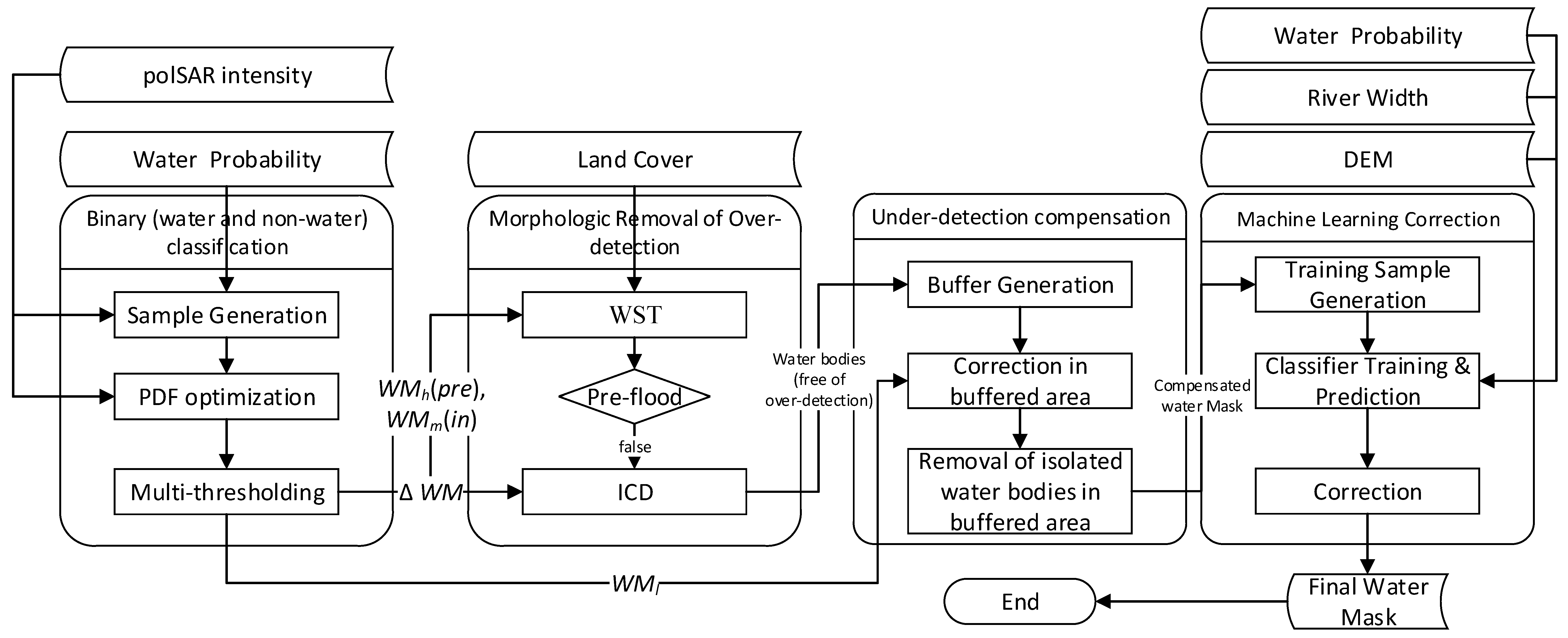
Shen et al. [59] developed a four-step processor, as shown in Figure 3, the Radar Produced Inundation Diary (RAPID), which makes use not only of time series of SAR data, but also the abundance of available high-resolution ancillary satellite products, including land cover classification (LCC) maps from Landsat [84,85], water occurrence from 30-year Landsat images [58], global river width from STRM [86] and Landsat images [87], and fine-resolution hydrography [88,89]. The four steps are as follows:

First, SAR images are classified into water and non-water masks (WMs), based on statistics from polarimetric radar. This binary classification step was inspired by the auto-optimization method by the m2b method [49] and extend to utilizing the dual-polarized SAR data. It removes the assumption of a bimodal distribution made in of m2b by initializing the water PDF using the water occurrence map.

Second, morphological processing runs over the mask, consisting of two operators, water source tracing (WST) and improved CD (ICD), to form inundated water bodies while to remove false positives caused by water-like surfaces. WST and ICD are also designed to detect fluvial and pluvial inundation, respectively. This morphological procedure is different from the post-processing methods in Matgen et al. [51], Chini et al. [77], and Twele et al. [90] in three aspects: (1) in RAPID, a pixel needs either to be accepted by WST or ICD while, in the other studies, the change detection is used to measure the pixels accepted by the RGA, which cannot capture pluvial inundated areas; (2) both WST and ICD utilize object-level information instead of pixel-level information to evaluate whether a detected water body is a false positive; and (3) to prevent the disturbance of calibration error among different SAR images, the change is detected from a binary mask instead of backscattering.

Third, a multi-threshold compensation step is applied to reduce the under-detection within water areas, and, fourth, a machine learning–based refinement is used to remove false negatives created by strong scatterers and to reduce further the noise level in the result. These final two steps in RAPID reduce the error caused by speckle and strong scatterers by utilizing the PDF and physically integrating multi-source remote sensing products instead of brutally applying a filtering technique. Thus, RAPID reduce the noise level without sacrificing resolution to mapping quality.

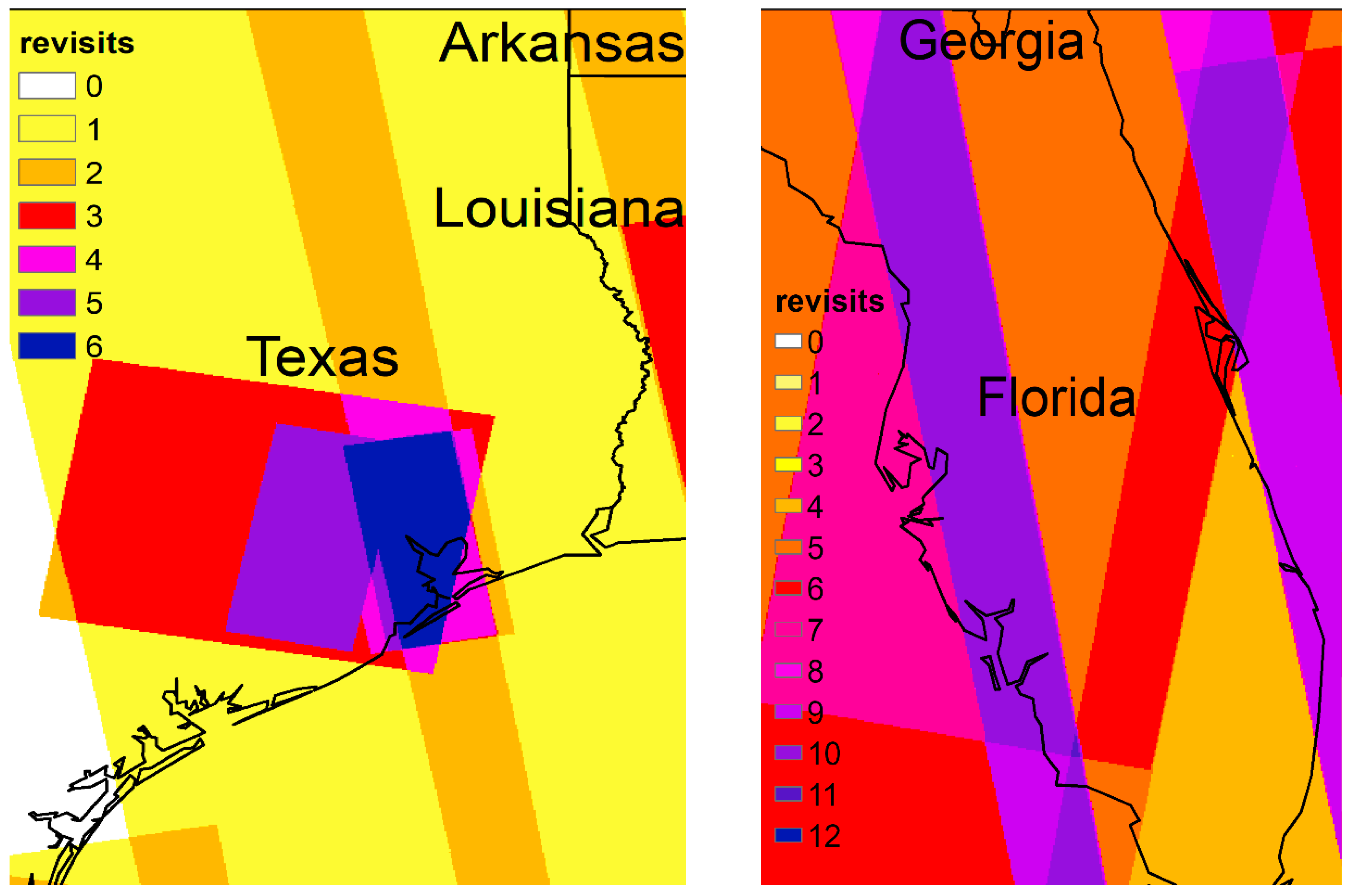
Among available satellites with SAR sensors, Sentinel-1 is the most popular because it is free to use and has relatively short revisiting intervals (six days in Europe and the Hawaiian islands and twelve days everywhere else in the world), three-day in average revisiting tracks (the revisiting intervals of the satellites (S1A and S1B) without the promise of producing the data), and a multi-year data archive dating back to 2014. During an event, the satellites may add extra revisits. As illustrated in Figure 4, for instance, for Hurricane Harvey six revisits were acquired from 27 August to 10 September 2017 in Seabrook area, and for Hurricane Irma eleven revisits from 12 September to 2 November 2017.

4. Summary

This study has reviewed existing principles and methods for inundation mapping using SAR data. As microwave measurements are significantly less disturbed by weather than measurements from optical sensors, SAR has the greater potential for high-resolution flood mapping. Efforts to automate the process leave a number of common errors unaddressed by most of the reviewed studies:

(1) The argument that flood maps resulting from region growing should include all “open water” pixels connected to the seeds may be untrue and lead to instances of under- and over- detection. If captured after the apex, large isolated and scattered flood pockets disconnected from the pre-flooded water bodies can develop at times due to variability in surface elevation and barriers. Limited by image resolution, narrow water paths or paths covered by vegetation may also appear isolated from known core water zones. Water-like areas can be connected to real water bodies as well; airports built, respectively, in Boston along the Atlantic Ocean and in San Francisco along the Pacific Ocean, for example, may be identified as water areas because they are water-like (smooth) and connected to real water bodies.

(2) Change detection at pixel level can eliminate false positives caused by water-like surfaces, but it is sensitive to noise-like speckle and geometric errors. In SAR applications, change detection approaches need to be applied with caution. Change in shadow areas, for instance, can be caused by change in the looking direction. Most studies that have used change detection models (including those reviewed here) have compared backscattering of collocated SAR pixels within and outside the flood period. Backscattering exhibits large heterogeneity in space and time, however, indicating that in a single object (water or non-water), the direct difference in backscattering might have led to erroneous interpretations. In addition, change detection was carried out from the output of RGA. Consequently, isolated inundation areas could not be detected.

(3) Although a speckle model has been taken into account by most studies, false positives and negatives caused by speckle pixels are not effectively reduced by other than brutal filtering techniques. More advanced approaches target on reducing the noisy effects without damaging image details, including selecting the optimal filter, simple morphological operators, multi-thresholding compensation, machine learning refinement and utilization of big EO data.

(4) Most approaches have not been tested in large areas, and their validation is usually limited to small areas along rivers. In particular, the limit of SAR-based mapping in terms of river width has not been reported. Limited by the 5–10 m resolution of noncommercial SAR satellites and the presence of speckle, one should not expect a successful rate in delineating inundation in headwater regions.

In the past decades, measurements based on satellite SAR have shifted from data scarcity to abundance. At present, Sentinel-1 enables new approaches taking advantage of big EO data by offering free and global SAR measurements from a large number of repeated observations. With its six-day revisiting intervals, however, Sentinel-1 alone cannot provide sufficiently frequent revisits for floods of short duration. More frequent scanning of the earth will be implemented by the constellation of SAR satellites (e.g., the four-satellite constellation of Cosmos SkyMed can provide revisits within a few hours) and planned SAR satellites (e.g., the NASA-ISRO SAR Satellite Mission (NISAR), planned to launch in 2020, is designed to provide spatiotemporal resolution of 5–10 m and four to six times per month). Consequently, newly emerging studies utilizing the big EO data have advanced to reduce the summarized error to a great extent.

As the automation of non-obstructed inundation extent has been fully addressed by previous studies, three topics may need further investigation: (1) the retrieval of inundation under vegetation; (2) the retrieval of urban inundation; and (3) the estimation of inundation depth from extent.

References

- Merwade, V.; Rajib, A.; Liu, Z. An integrated approach for flood inundation modeling on large scales. In Bridging Science and Policy Implication for Managing Climate Extremes; Jung, H.-S., Wang, B., Eds.; World Scientific Publication Company: Singapore, 2018; pp. 133–155. [Google Scholar]
- Wing, O.E.; Bates, P.D.; Smith, A.M.; Sampson, C.C.; Johnson, K.A.; Fargione, J.; Morefield, P. Estimates of present and future flood risk in the conterminous united states. Environ. Res. Lett. 2018, 13, 1748–9326. [Google Scholar] [CrossRef]
- Yamazaki, D.; Kanae, S.; Kim, H.; Oki, T. A physically based description of floodplain inundation dynamics in a global river routing model. Water Resour. Res. 2011, 47. [Google Scholar] [CrossRef] [Green Version]
- Hardesty, S.; Shen, X.; Nikolopoulos, E.; Anagnostou, E. A numerical framework for evaluating flood inundation risk under different dam operation scenarios. Water 2018, 10, 1798. [Google Scholar] [CrossRef]
- Shen, X.; Hong, Y.; Zhang, K.; Hao, Z. Refining a distributed linear reservoir routing method to improve performance of the crest model. J. Hydrol. Eng. 2016, 22. [Google Scholar] [CrossRef]
- Shen, X.; Hong, Y.; Anagnostou, E.N.; Zhang, K.; Hao, Z. Chapter 7 an advanced distributed hydrologic framework-the development of crest. In Hydrologic Remote Sensing and Capacity Building, Chapter; Hong, Y., Zhang, Y., Khan, S.I., Eds.; CRC Press: Boca Raton, FL, USA, 2016; pp. 127–138. [Google Scholar]
- Shen, X.; Anagnostou, E.N. A framework to improve hyper-resolution hydrologic simulation in snow-affected regions. J. Hydrol. 2017, 552, 1–12. [Google Scholar] [CrossRef]
- Afshari, S.; Tavakoly, A.A.; Rajib, M.A.; Zheng, X.; Follum, M.L.; Omranian, E.; Fekete, B.M. Comparison of new generation low-complexity flood inundation mapping tools with a hydrodynamic model. J. Hydrol. 2018, 556, 539–556. [Google Scholar] [CrossRef]
- Horritt, M.; Bates, P. Evaluation of 1d and 2d numerical models for predicting river flood inundation. J. Hydrol. 2002, 268, 87–99. [Google Scholar] [CrossRef]
- Liu, Z.; Merwade, V.; Jafarzadegan, K. Investigating the role of model structure and surface roughness in generating flood inundation extents using one-and two-dimensional hydraulic models. J. Flood Risk Manag. 2018, 12, e12347. [Google Scholar] [CrossRef]
- Zheng, X.; Lin, P.; Keane, S.; Kesler, C.; Rajib, A. Nhdplus-Hand Evaluation; Consortium of Universities for the Advancement of Hydrologic Science, Inc.: Boston, MA, USA, 2016; p. 122. [Google Scholar]
- Dodov, B.; Foufoula-Georgiou, E. Floodplain morphometry extraction from a high-resolution digital elevation model: A simple algorithm for regional analysis studies. Geosci. Remote Sens. Lett. IEEE 2006, 3, 410–413. [Google Scholar] [CrossRef]
- Nardi, F.; Biscarini, C.; Di Francesco, S.; Manciola, P.; Ubertini, L. Comparing a large-scale dem-based floodplain delineation algorithm with standard flood maps: The tiber river basin case study. Irrig. Drain. 2013, 62, 11–19. [Google Scholar] [CrossRef]
- Shen, X.; Vergara, H.J.; Nikolopoulos, E.I.; Anagnostou, E.N.; Hong, Y.; Hao, Z.; Zhang, K.; Mao, K. Gdbc: A tool for generating global-scale distributed basin morphometry. Environ. Model. Softw. 2016, 83, 212–223. [Google Scholar] [CrossRef]
- Shen, X.; Anagnostou, E.N.; Mei, Y.; Hong, Y. A global distributed basin morphometric dataset. Sci. Data 2017, 4, 160124. [Google Scholar] [CrossRef] [Green Version]
- Shen, X.; Mei, Y.; Anagnostou, E.N. A comprehensive database of flood events in the contiguous united states from 2002 to 2013. Bull. Am. Meteorol. Soc. 2017, 98, 1493–1502. [Google Scholar] [CrossRef]
- Cohen, S.; Brakenridge, G.R.; Kettner, A.; Bates, B.; Nelson, J.; McDonald, R.; Huang, Y.F.; Munasinghe, D.; Zhang, J. Estimating floodwater depths from flood inundation maps and topography. JAWRA J. Am. Water Resour. Assoc. 2017, 54, 847–858. [Google Scholar] [CrossRef]
- Nguyen, N.Y.; Ichikawa, Y.; Ishidaira, H. Estimation of inundation depth using flood extent information and hydrodynamic simulations. Hydrol. Res. Lett. 2016, 10, 39–44. [Google Scholar] [CrossRef]
- Cian, F.; Marconcini, M.; Ceccato, P.; Giupponi, C.J.N.H.; Sciences, E.S. Flood depth estimation by means of high-resolution sar images and lidar data. Nat. Hazards Earth Syst. Sci. 2018, 18, 3063–3084. [Google Scholar] [CrossRef]
- Shen, X.; Anagnostou, E. Rapid sar-based flood-inundation extent/depth estimation. In Proceedings of the AGU Fall Meeting 2018, Washington, DC, USA, 11–15 December 2018. [Google Scholar]
- Jones, J. The us geological survey dynamic surface water extent product evaluation strategy. In Proceedings of the EGU General Assembly Conference Abstracts, Vienna, Austria, 17–22 April 2016; Volume 18, p. 8197. [Google Scholar]
- Jones, J.W. Efficient wetland surface water detection and monitoring via landsat: Comparison with in situ data from the everglades depth estimation network. Remote Sens. 2015, 7, 12503–12538. [Google Scholar] [CrossRef]
- Heimhuber, V.; Tulbure, M.G.; Broich, M. Modeling multidecadal surface water inundation dynamics and key drivers on large river basin scale using multiple time series of earth-observation and river flow data. Water Resour. Res. 2017, 53, 1251–1269. [Google Scholar] [CrossRef]
- Jones, J.W. Improved automated detection of subpixel-scale inundation—Revised dynamic surface water extent (dswe) partial surface water tests. Remote Sens. 2019, 11, 374. [Google Scholar] [CrossRef]
- Papa, F.; Prigent, C.; Aires, F.; Jimenez, C.; Rossow, W.; Matthews, E. Interannual variability of surface water extent at the global scale, 1993–2004. J. Geophys. Res. Atmos. 2010, 115. [Google Scholar] [CrossRef] [Green Version]
- Prigent, C.; Papa, F.; Aires, F.; Rossow, W.B.; Matthews, E. Global inundation dynamics inferred from multiple satellite observations, 1993–2000. J. Geophys. Res. Atmos. 2007, 112. [Google Scholar] [CrossRef] [Green Version]
- Aires, F.; Papa, F.; Prigent, C.; Crétaux, J.-F.; Berge-Nguyen, M. Characterization and space–time downscaling of the inundation extent over the inner niger delta using giems and modis data. J. Hydrometeorol. 2014, 15, 171–192. [Google Scholar] [CrossRef]
- Takbiri, Z.; Ebtehaj, A.M.; Foufoula-Georgiou, E.J. A multi-sensor data-driven methodology for all-sky passive microwave inundation retrieval. arXiv, 2018; arXiv:1807.03803. [Google Scholar]
- Shen, X.; Hong, Y.; Qin, Q.; Chen, S.; Grout, T. A backscattering enhanced canopy scattering model based on mimics. In Proceedings of the American Geophysical Union (AGU) 2010 Fall Meeting, San Francisco, CA, USA, 13–17 December 2010. [Google Scholar]
- Ulaby, F.T.; Moore, R.K.; Fung, A.K. Microwave Remote Sensing: Active and Passive; Artech House Inc.: London, UK, 1986; Volume 3, p. 1848. [Google Scholar]
- Fung, A.K. Microwave Scattering and Emission Models and Their Applications; Artech House: Cambridge, UK; New York, NY, USA, 1994. [Google Scholar]
- Refice, A.; Capolongo, D.; Pasquariello, G.; D’Addabbo, A.; Bovenga, F.; Nutricato, R.; Lovergine, F.P.; Pietranera, L. Sar and insar for flood monitoring: Examples with cosmo-skymed data. IEEE J. Sel. Top. Appl. Earth Obs. Remote Sens. 2014, 7, 2711–2722. [Google Scholar] [CrossRef]
- Pulvirenti, L.; Chini, M.; Pierdicca, N.; Boni, G. Use of sar data for detecting floodwater in urban and agricultural areas: The role of the interferometric coherence. IEEE Trans. Geosci. Remote Sens. 2016, 54, 1532–1544. [Google Scholar] [CrossRef]
- Chini, M.; Papastergios, A.; Pulvirenti, L.; Pierdicca, N.; Matgen, P.; Parcharidis, I. Sar coherence and polarimetric information for improving flood mapping. In Proceedings of the 2016 IEEE International Geoscience and Remote Sensing Symposium (IGARSS), Beijing, China, 10–15 July 2016; pp. 7577–7580. [Google Scholar]
- Chini, M.; Pelich, R.; Pulvirenti, L.; Pierdicca, N.; Hostache, R.; Matgen, P. Sentinel-1 insar coherence to detect floodwater in urban areas: Houston and hurricane harvey as a test case. Remote Sens. 2019, 11, 107. [Google Scholar] [CrossRef]
- Schumann, G.J.-P.; Moller, D.K. Microwave remote sensing of flood inundation. Phys. Chem. Earthparts A/B/C 2015, 83, 84–95. [Google Scholar] [CrossRef]
- Gray, A.L.; Vachon, P.W.; Livingstone, C.E.; Lukowski, T.I. Synthetic aperture radar calibration using reference reflectors. IEEE Trans. Geosci. Remote Sens. 1990, 28, 374–383. [Google Scholar] [CrossRef]
- Lee, J.S.; Pottier, E. Polarimetric Radar Imaging: From Basics to Applications; CRC: Boca Raton, FL, USA, 2009. [Google Scholar]
- Gomez, L.; Ospina, R.; Frery, A.C. Statistical properties of an unassisted image quality index for sar imagery. Remote Sens. 2019, 11, 385. [Google Scholar] [CrossRef]
- Borghys, D.; Yvinec, Y.; Perneel, C.; Pizurica, A.; Philips, W. Supervised feature-based classification of multi-channel sar images. Pattern Recognit. Lett. 2006, 27, 252–258. [Google Scholar] [CrossRef]
- Kussul, N.; Shelestov, A.; Skakun, S. Grid system for flood extent extraction from satellite images. Earth Sci. Inform. 2008, 1, 105. [Google Scholar] [CrossRef]
- Pulvirenti, L.; Pierdicca, N.; Chini, M. Analysis of cosmo-skymed observations of the 2008 flood in myanmar. Ital. J. Remote Sens. 2010, 42, 79–90. [Google Scholar] [CrossRef]
- Song, Y.-S.; Sohn, H.-G.; Park, C.-H. Efficient water area classification using radarsat-1 sar imagery in a high relief mountainous environment. Photogramm. Eng. Remote Sens. 2007, 73, 285–296. [Google Scholar] [CrossRef]
- Townsend, P.A. Mapping seasonal flooding in forested wetlands using multi-temporal radarsat sar. Photogramm. Eng. Remote Sens. 2001, 67, 857–864. [Google Scholar]
- Töyrä, J.; Pietroniro, A.; Martz, L.W.; Prowse, T.D. A multi-sensor approach to wetland flood monitoring. Hydrol. Process. 2002, 16, 1569–1581. [Google Scholar] [CrossRef]
- Zhou, C.; Luo, J.; Yang, C.; Li, B.; Wang, S. Flood monitoring using multi-temporal avhrr and radarsat imagery. Photogramm. Eng. Remote Sens. 2000, 66, 633–638. [Google Scholar]
- Pulvirenti, L.; Pierdicca, N.; Chini, M.; Guerriero, L. An algorithm for operational flood mapping from synthetic aperture radar (sar) data using fuzzy logic. Nat. Hazards Earth Syst. Sci. 2011, 11, 529. [Google Scholar] [CrossRef]
- Yamada, Y. Detection of flood-inundated area and relation between the area and micro-geomorphology using sar and gis. In Proceedings of the IGARSS’01, IEEE 2001 International Conference on Geoscience and Remote Sensing Symposium, Sydney, NSW, Australia, 9–13 July 2001; pp. 3282–3284. [Google Scholar]
- Giustarini, L.; Hostache, R.; Matgen, P.; Schumann, G.J.-P.; Bates, P.D.; Mason, D.C. A change detection approach to flood mapping in urban areas using terrasar-x. Geosci. Remote Sens. IEEE Trans. 2013, 51, 2417–2430. [Google Scholar] [CrossRef]
- Hirose, K.; Maruyama, Y.; Do Van, Q.; Tsukada, M.; Shiokawa, Y. Visualization of flood monitoring in the lower reaches of the mekong river. In Proceedings of the 22nd Asian Conference on Remote Sensing, Singapore, 5–9 Novembers 2001; p. 9. [Google Scholar]
- Matgen, P.; Hostache, R.; Schumann, G.; Pfister, L.; Hoffmann, L.; Savenije, H. Towards an automated sar-based flood monitoring system: Lessons learned from two case studies. Phys. Chem. Earthparts A/B/C 2011, 36, 241–252. [Google Scholar] [CrossRef]
- Tan, Q.; Bi, S.; Hu, J.; Liu, Z. Measuring lake water level using multi-source remote sensing images combined with hydrological statistical data. In Proceedings of the IGARSS’04, 2004 IEEE International Conference on Geoscience and Remote Sensing Symposium, Anchorage, AK, USA, 20–24 September 2004; pp. 4885–4888. [Google Scholar]
- Martinis, S.; Twele, A.; Voigt, S. Towards operational near real-time flood detection using a split-based automatic thresholding procedure on high resolution terrasar-x data. Nat. Hazards Earth Syst. Sci. 2009, 9, 303–314. [Google Scholar] [CrossRef]
- Martinis, S.; Rieke, C. Backscatter analysis using multi-temporal and multi-frequency sar data in the context of flood mapping at river saale, germany. Remote Sens. 2015, 7, 7732–7752. [Google Scholar] [CrossRef]
- Bovolo, F.; Bruzzone, L. A split-based approach to unsupervised change detection in large-size multitemporal images: Application to tsunami-damage assessment. IEEE Trans. Geosci. Remote Sens. 2007, 45, 1658–1670. [Google Scholar] [CrossRef]
- Baatz, M. Object-oriented and multi-scale image analysis in semantic networks. In Proceedings of the the 2nd International Symposium on Operationalization of Remote Sensing, Enschede, The Netherlands, 16–20 August 1999. [Google Scholar]
- Lu, J.; Giustarini, L.; Xiong, B.; Zhao, L.; Jiang, Y.; Kuang, G. Automated flood detection with improved robustness and efficiency using multi-temporal sar data. Remote Sens. Lett. 2014, 5, 240–248. [Google Scholar] [CrossRef]
- Pekel, J.-F.; Cottam, A.; Gorelick, N.; Belward, A.S. High-resolution mapping of global surface water and its long-term changes. Nature 2016, 540, 418–422. [Google Scholar] [CrossRef]
- Shen, X.; Anagnostou, E.N.; Allen, G.H.; Brakenridge, G.R.; Kettner, A.J. Near real-time nonobstructed flood inundation mapping by synthetic aperture radar. Remote Sens. Environ. 2019, 221, 302–335. [Google Scholar] [CrossRef]
- Horritt, M. A statistical active contour model for sar image segmentation. Image Vis. Comput. 1999, 17, 213–224. [Google Scholar] [CrossRef]
- Horritt, M.S.; Mason, D.C.; Luckman, A.J. Flood boundary delineation from synthetic aperture radar imagery using a statistical active contour model. Int. J. Remote Sens. 2001, 22, 2489–2507. [Google Scholar] [CrossRef]
- Heremans, R.; Willekens, A.; Borghys, D.; Verbeeck, B.; Valckenborgh, J.; Acheroy, M.; Perneel, C. Automatic detection of flooded areas on envisat/asar images using an object-oriented classification technique and an active contour algorithm. In Proceedings of the RAST’03, International Conference on Recent Advances in Space Technologies, Istanbul, Turkey, 20–22 November 2003; pp. 311–316. [Google Scholar]
- Pulvirenti, L.; Chini, M.; Pierdicca, N.; Guerriero, L.; Ferrazzoli, P. Flood monitoring using multi-temporal cosmo-skymed data: Image segmentation and signature interpretation. Remote Sens. Environ. 2011, 115, 990–1002. [Google Scholar] [CrossRef]
- Santoro, M.; Wegmüller, U. Multi-temporal sar metrics applied to map water bodies. In Proceedings of the 2012 IEEE International Conference on Geoscience and Remote Sensing Symposium (IGARSS), Munich, Germany, 22–27 July 2012; pp. 5230–5233. [Google Scholar]
- Bazi, Y.; Bruzzone, L.; Melgani, F. An unsupervised approach based on the generalized gaussian model to automatic change detection in multitemporal sar images. IEEE Trans. Geosci. Remote Sens. 2005, 43, 874–887. [Google Scholar] [CrossRef]
- Landuyt, L.; Van Wesemael, A.; Schumann, G.J.; Hostache, R.; Verhoest, N.E.; Van Coillie, F.M. Flood mapping based on synthetic aperture radar: An assessment of established approaches. IEEE Trans. Geosci. Remote 2018, 57, 1–18. [Google Scholar] [CrossRef]
- Cian, F.; Marconcini, M.; Ceccato, P. Normalized difference flood index for rapid flood mapping: Taking advantage of eo big data. Remote Sens. Environ. 2018, 209, 712–730. [Google Scholar] [CrossRef]
- Horritt, M.S.; Mason, D.C.; Cobby, D.M.; Davenport, I.J.; Bates, P.D. Waterline mapping in flooded vegetation from airborne sar imagery. Remote Sens. Environ. 2003, 85, 271–281. [Google Scholar] [CrossRef]
- Pulvirenti, L.; Pierdicca, N.; Chini, M.; Guerriero, L. Monitoring flood evolution in vegetated areas using cosmo-skymed data: The tuscany 2009 case study. IEEE J. Sel. Top. Appl. Earth Obs. Remote Sens. 2013, 6, 1807–1816. [Google Scholar] [CrossRef]
- Ormsby, J.P.; Blanchard, B.J.; Blanchard, A.J. Detection of lowland flooding using active microwave systems. Photogramm. Eng. Remote Sens. 1985, 51, 317–328. [Google Scholar]
- Mason, D.C.; Davenport, I.J.; Neal, J.C.; Schumann, G.J.-P.; Bates, P.D. Near real-time flood detection in urban and rural areas using high-resolution synthetic aperture radar images. IEEE Trans. Geosci. Remote Sens. 2012, 50, 3041–3052. [Google Scholar] [CrossRef]
- Mason, D.C.; Speck, R.; Devereux, B.; Schumann, G.J.-P.; Neal, J.C.; Bates, P.D. Flood detection in urban areas using terrasar-x. IEEE Trans. Geosci. Remote Sens. 2010, 48, 882–894. [Google Scholar] [CrossRef]
- Mason, D.C.; Giustarini, L.; Garcia-Pintado, J.; Cloke, H.L. Detection of flooded urban areas in high resolution synthetic aperture radar images using double scattering. Int. J. Appl. Earth Obs. Geoinf. 2014, 28, 150–159. [Google Scholar] [CrossRef]
- Ferro, A.; Brunner, D.; Bruzzone, L.; Lemoine, G. On the relationship between double bounce and the orientation of buildings in vhr sar images. IEEE Geosci. Remote Sens. Lett. 2011, 8, 612–616. [Google Scholar] [CrossRef]
- Kittler, J.; Illingworth, J. Minimum error thresholding. Pattern Recognit. 1986, 19, 41–47. [Google Scholar] [CrossRef]
- Martinis, S.; Kersten, J.; Twele, A. A fully automated terrasar-x based flood service. Isprs J. Photogramm. Remote Sens. 2015, 104, 203–212. [Google Scholar] [CrossRef]
- Chini, M.; Hostache, R.; Giustarini, L.; Matgen, P. A hierarchical split-based approach for parametric thresholding of sar images: Flood inundation as a test case. IEEE Trans. Geosci. Remote Sens. 2017, 55, 6975–6988. [Google Scholar] [CrossRef]
- Bracaglia, M.; Ferrazzoli, P.; Guerriero, L. A fully polarimetric multiple scattering model for crops. Remote Sens. Environ. 1995, 54, 170–179. [Google Scholar] [CrossRef]
- Fung, A.K.; Shah, M.R.; Tjuatja, S. Numerical simulation of scattering from three-dimensional randomly rough surfaces. Geosci. Remote Sens. IEEE Trans. 1994, 32, 986–994. [Google Scholar] [CrossRef]
- Chini, M.; Pelich, R.; Hostache, R.; Matgen, P.; Lopez-Martinez, C. Towards a 20 m global building map from sentinel-1 sar data. Remote Sens. 2018, 10, 1833. [Google Scholar] [CrossRef]
- Freeman, A.; Durden, S.L. A three-component scattering model for polarimetric sar data. IEEE Trans. Geosci. Remote Sens. 1998, 36, 963–973. [Google Scholar] [CrossRef]
- Yamaguchi, Y.; Moriyama, T.; Ishido, M.; Yamada, H. Four-component scattering model for polarimetric sar image decomposition. IEEE Trans. Geosci. Remote Sens. 2005, 43, 1699–1706. [Google Scholar] [CrossRef]
- Giustarini, L.; Hostache, R.; Kavetski, D.; Chini, M.; Corato, G.; Schlaffer, S.; Matgen, P. Probabilistic flood mapping using synthetic aperture radar data. IEEE Trans. Geosci. Remote Sens. 2016, 54, 6958–6969. [Google Scholar] [CrossRef]
- Fry, J.A.; Xian, G.; Jin, S.; Dewitz, J.A.; Homer, C.G.; Limin, Y.; Barnes, C.A.; Herold, N.D.; Wickham, J.D. Completion of the 2006 national land cover database for the conterminous united states. Photogramm. Eng. Remote Sens. 2011, 77, 858–864. [Google Scholar]
- Gong, P.; Wang, J.; Yu, L.; Zhao, Y.; Zhao, Y.; Liang, L.; Niu, Z.; Huang, X.; Fu, H.; Liu, S. Finer resolution observation and monitoring of global land cover: First mapping results with landsat tm and etm+ data. Int. J. Remote Sens. 2013, 34, 2607–2654. [Google Scholar] [CrossRef]
- Yamazaki, D.; O’Loughlin, F.; Trigg, M.A.; Miller, Z.F.; Pavelsky, T.M.; Bates, P.D. Development of the global width database for large rivers. Water Resour. Res. 2014, 50, 3467–3480. [Google Scholar] [CrossRef]
- Allen, G.H.; Pavelsky, T.M. Global extent of rivers and streams. Science 2018, 361, 585–588. [Google Scholar] [CrossRef]
- Simley, J.D.; Carswell, W.J., Jr. The National Map—Hydrography; U.S. Geological Survey: Reston, VA, USA, 2009.
- Yamazaki, D.; Ikeshima, D.; Tawatari, R.; Yamaguchi, T.; O’Loughlin, F.; Neal, J.C.; Sampson, C.C.; Kanae, S.; Bates, P.D. A high-accuracy map of global terrain elevations. Geophys. Res. Lett. 2017, 44, 5844–5853. [Google Scholar] [CrossRef] [Green Version]
- Twele, A.; Cao, W.; Plank, S.; Martinis, S. Sentinel-1-based flood mapping: A fully automated processing chain. Int. J. Remote Sens. 2016, 37, 2990–3004. [Google Scholar] [CrossRef]
Figure 1.
Backscattering components from vegetation with a canopy layer in enhanced MIMICS.
Figure 2.
(a) Vertical and (b) horizontal swipe demonstration of the geometric error (circulated tracks) between two Sentinel-1 SAR images georeferenced by Range-Doppler algorithm in Sentinel Application Platform (SNAP) 6.0 software using the Shuttle Radar Topography Mission (STRM) 3’’ DEM data. The background and foreground images were obtained, respectively, over George Bush International Airport, Texas.
Figure 3.
The workflow of RAPID. From the left to the right panels are step 1 (binary classification), 2 (morphological processing consisting of water source tracing (WST) and improved change detection (ICD), 3 (multi-threshold compensation) and 4 (machine-learning-based correction), respectively.
Figure 4.
During Harvey, (a) Sentinel-1 SAR data availability days and coverage in Texas and (b) the inundated times of the Seabrook area.
© 2019 by the authors. Licensee MDPI, Basel, Switzerland. This article is an open access article distributed under the terms and conditions of the Creative Commons Attribution (CC BY) license (http://creativecommons.org/licenses/by/4.0/).
Share and Cite
MDPI and ACS Style
Shen, X.; Wang, D.; Mao, K.; Anagnostou, E.; Hong, Y. Inundation Extent Mapping by Synthetic Aperture Radar: A Review. Remote Sens. 2019, 11, 879. https://0-doi-org.brum.beds.ac.uk/10.3390/rs11070879
AMA Style
Shen X, Wang D, Mao K, Anagnostou E, Hong Y. Inundation Extent Mapping by Synthetic Aperture Radar: A Review. Remote Sensing. 2019; 11(7):879. https://0-doi-org.brum.beds.ac.uk/10.3390/rs11070879
Chicago/Turabian StyleShen, Xinyi, Dacheng Wang, Kebiao Mao, Emmanouil Anagnostou, and Yang Hong. 2019. "Inundation Extent Mapping by Synthetic Aperture Radar: A Review" Remote Sensing 11, no. 7: 879. https://0-doi-org.brum.beds.ac.uk/10.3390/rs11070879
Note that from the first issue of 2016, this journal uses article numbers instead of page numbers. See further details here.