Improving Jujube Fruit Tree Yield Estimation at the Field Scale by Assimilating a Single Landsat Remotely-Sensed LAI into the WOFOST Model

Abstract

Few studies were focused on yield estimation of perennial fruit tree crops by integrating remotely-sensed information into crop models. This study presented an attempt to assimilate a single leaf area index (LAI) near to maximum vegetative development stages derived from Landsat satellite data into a calibrated WOFOST model to predict yields for jujube fruit trees at the field scale. Field experiments were conducted in three growth seasons to calibrate input parameters for WOFOST model, with a validated phenology error of −2, −3, and −3 days for emergence, flowering, and maturity, as well as an R² of 0.986 and RMSE of 0.624 t ha⁻¹ for total aboveground biomass (TAGP), R² of 0.95 and RMSE of 0.19 m² m⁻² for LAI, respectively. Normalized Difference Vegetation Index (NDVI) showed better performance for LAI estimation than a Soil-adjusted Vegetation Index (SAVI), with a better agreement (R² = 0.79) and prediction accuracy (RMSE = 0.17 m² m⁻²). The assimilation after forcing LAI improved the yield prediction accuracy compared with unassimilated simulation and remotely sensed NDVI regression method, showing a R² of 0.62 and RMSE of 0.74 t ha⁻¹ for 2016, and R² of 0.59 and RMSE of 0.87 t ha⁻¹ for 2017. This research would provide a strategy to employ remotely sensed state variables and a crop growth model to improve field-scale yield estimates for fruit tree crops.

1. Introduction

Jujube tree (Zizyphus jujube) is an important economic tree species, which is mainly cultivated in the subtropical and tropical regions in Asia and America with a history of more than 3000 years. The economic jujube forest plays an important role in protecting crops or vegetables grown during the dry season, such as wind break and sand fixation [1]. In addition, its fruit not only has important nutritional value, such as vitamin C, amino acids, carbohydrate, and minerals, but also has significant medical value, like tonic medicine for blood nourishment, and analeptic and palliative uses [2]. The Xinjiang Uygur Autonomous Region of China is the main production area of jujube fruits (>500,000 hectares) due to excellent light and heat conditions. The yield in 2016 is more than 3.2 million tons (Xinjiang Statistical Yearbook, 2017). With the expansion of the cultivated area, the regional scale yield prediction before harvest is essential for national planting policies, food security, and export strategies. More importantly, the field-scale jujube growth and yield estimates before harvest allow farmers to improve yield management decision-making, such as irrigation, fertilization, pruning, and density selection, which is also an important research topic of precision agriculture and forestry.

Cropping systems modelling based on mathematical descriptions expresses and quantifies the crop development process influenced by climate, soil and management conditions, which has been considered as a mature method for yield prediction [3]. Over the past decades, such crop models have been developed for different crops and purposes, and prominent models are WOFOST (WOrld FOod STudies) [4], DSSAT (Decision Support System for Agrotechnology Transfer) [5], EPIC (Environmental Policy Integrated Climate) [6], STICS (Multidisciplinary simulator for standard crops) [7], APSIM (Agricultural Production Systems sIMulator) [8], SWAP (Soil, Water, Atmosphere and Plant) [9], AquaCrop (Crop-water productivity model) [10], and CropSyst (Cropping Systems Simulation Model) [11]. However, the spatial variation of input parameters of such models shall be accounted for when crop yields are estimated over large regions [12]. The uncertainties of soil properties (soil moisture and field capacity, etc.), initial and canopy state variables (sowing date, initial dry weight, LAI, biomass, etc.) may affect the accuracy of crop growth simulation and yield assessment [3,13].

Remote sensing (RS) data can provide information about meteorological, vegetation, and soil conditions in large areas. Initial input parameters, state variables or soil properties for crop model over large areas, such as LAI [14,15,16,17], biomass [18], leaf nitrogen accumulation [19], evapotranspiration [20,21], and soil moisture [22,23,24], can be observed from remote sensing data. These variables have often used to integrate with crop models to adjust and optimize some important input parameters and state variables to improve simulation results at field and regional scales. Remote sensing has also been employed to accurately monitor crop phenology to improve crop model outcomes because phenological information controls crop biomass accumulation length and distribution during growth period [25]. In the last 10–15 years, more new satellite data is available, such as optical remote sensing data with medium and high spatial and temporal resolution (Sentinel-2; Landsat 8; RapidEye; WorldView-2; SPOT-6; GeoEye-1; Huanjing-1; Gaofen-1; et al.) and radar satellite data (ENVISAT, Sentinal-1, ALOS, ALOS-2, RADARSAT-2, TERRASAR-X, COSMO, etc.). They provide more timely and reliable data for crop model inputs [12].

Assimilation methods are often used to integrate remote sensing data into crop growth models, mainly including calibration methods, forcing methods, and updating methods [26,27,28,29]. In general, the main purpose of assimilation is to integrate canopy state variables or soil properties that are closely related to the crop growth process to optimize the key input parameters for the crop model. The methods have been employed to improve the prediction accuracy of crop yields at a regional scale [21,22,30,31,32,33,34,35,36,37] and at a field scale [38,39,40,41,42].

For calibration methods, an optimization algorithm is performed to minimize the difference between the remote sensing observation values and the crop model simulation values for re-calibrating and optimizing input parameters of crop models. The main optimization algorithms include the Maximum Likelihood Solution (MLS) [22], simplex search algorithm [43], Least Squares Method (LSM) [44], Powell’s conjugate direction method (PCDM) [45], Shuffled Complex Evolution (SCE-UA) [21,46], Very Fast Annealing Algorithm (VFSA) [47], and Particle Swarm Optimization Algorithm (PSO) [48]. For forcing methods, the crop model simulation value is directly replaced by the remotely-sensed value as a state variable to improve the simulated result [12], such as LAI, aboveground biomass (AGB), yield, transpiration [17,49,50,51,52] and flowering date [53]. The updating method focuses on continuously updating crop model simulation data, mainly including Kalman Filter (KF) [54,55], Ensemble Kalman Filter (EnKF) [56], Three-Dimensional Variational Data Assimilation (3DVAR) [57], Four-Dimensional Variational Data Assimilation (4DVAR) [58], Particle Filter (PF) [59], and Hierarchical Bayesian Method (HBM) [60,61]. The correct orthogonal decomposition technique and the aggregate square root filtering method in EnKF, 4DVar, PF, and 4DVar (POD4DVar) are used to combine the state variables of the remote sensing data and the crop model with the estimated soil moisture, AGB, LAI, and yield [62,63,64]. In short, it is generally believed that the yield prediction based on crop models can be improved by combining biophysical variables from remotely-sensed data during the growing period [13].

However, almost all crop growth models and assimilation methods have been employed and improved for annual crops, few studies are focused on production simulation and assimilation of perennial fruit trees. Although existing research has confirmed that crop growth model (WOFOST) can be used to simulate jujube growth in field experiments by calibrating input parameters [65], the difference in actual tree age and planting density at different fields may be also uncertain. The difference shows a strong influence on jujube yield. In theory, the initial dry matter weight (TDWI) parameter of the WOFOST model can respond to the effect of these two factors on yield. The main objective of this study was to use remote sensing assimilation method to reduce the uncertainty of key input parameter (TDWI) associated with tree age and planting density and improve yield prediction accuracy at field scale. To accomplish this goal, the following specific objectives were defined:

(1) To calibrate and validate input parameters for jujube simulation based on WOFOST model, and re-calibrate TDWIs for field-scale jujube orchards by forcing LAI derived from Landsat 8 data;

(2) To explore whether a single LAI (near to the max vegetative development stages) obtained from Landsat 8 with medium spatial resolution can improve the yield simulation accuracy for a fruit tree crop;

(3) To evaluate the assimilation performance at field scale by comparing the yield prediction results before and after forcing LAI, as well as directly using remotely-sensed regression methods.

2. Materials and Methods

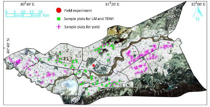
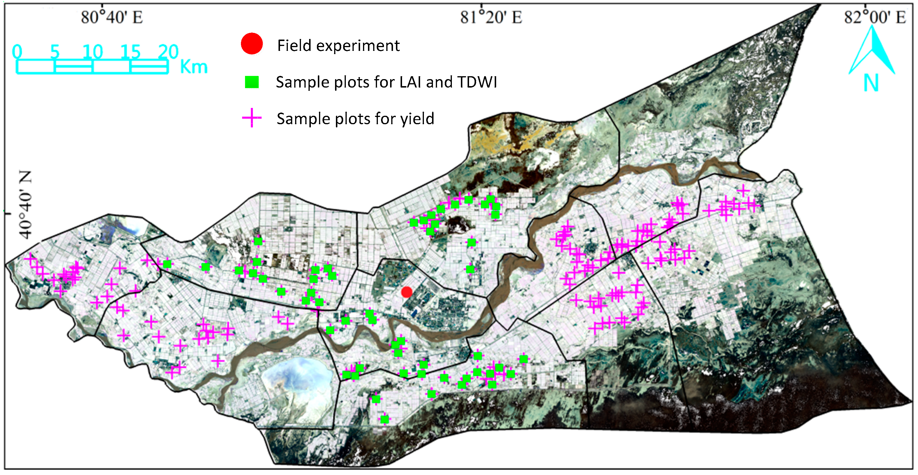
2.1. Study Region

The study was conducted in Alaer City (80°30′E–81°58′E, 40°22′N–40°57′N) in Western China with large planting areas of jujube. This city planted about 50,000 hectares and produces almost one-eighth of the national total dry jujube, and consists of 10 ecoregions. Sampled jujube orchards were cultivated between 2007 and 2014, with a planting density ranging from 2000–10,000 trees per hectare. The climate was arid warm-temperate climate with an average annual rainfall from 40 mm to 98 mm. The soil texture was primarily a sandy loam. An average temperature ranged from 10.6 °C to 29.3 °C during the main growth period (from April–October). The jujube trees usually begin to emerge in mid-April, and the fruits mature in early October and are harvested in early November. Figure 1 shows the study area and the distribution of the field observation spots.

2.2. Research Framework

The core of our strategy was to force a single LAI near to the max vegetative development stages from Landsat 8 remote sensing data into the WOFOST model to improve the jujube yield prediction accuracy at field scale, and compare the forecasting performance before and after the forced LAI, and directly using the remote sensing vegetation index regression method. The research mainly included four key steps.

• Model calibration and yield prediction without forcing LAI: The WOFOST model parameters were calibrated and validated using field experimental data (jujube, soil, and weather data). Default values calculated using the planting density of each orchard multiplied by the average TDWI per tree were input into the calibrated model to predict yields of 181 orchard samples.
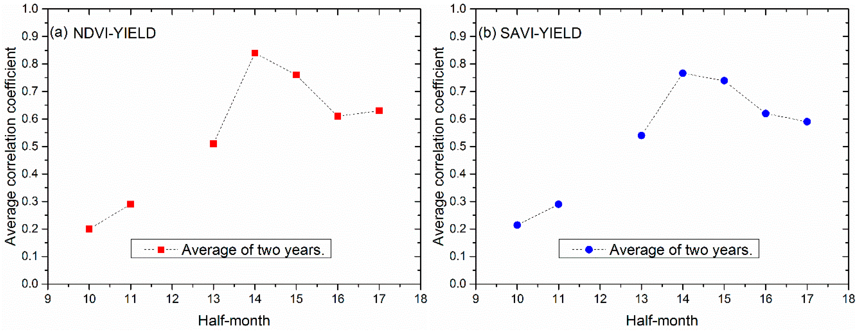
• Yield prediction using remotely-sensed vegetation indices (VIs): The correlations between the vegetation index obtained from Landsat data during the main growing period and yield data were analyzed to determine the best modeling time. A single or composite vegetation index with highest correlation was chosen to establish the yield prediction model for 181 sample spots. The prediction accuracy was cross-validated using two years of yield data.
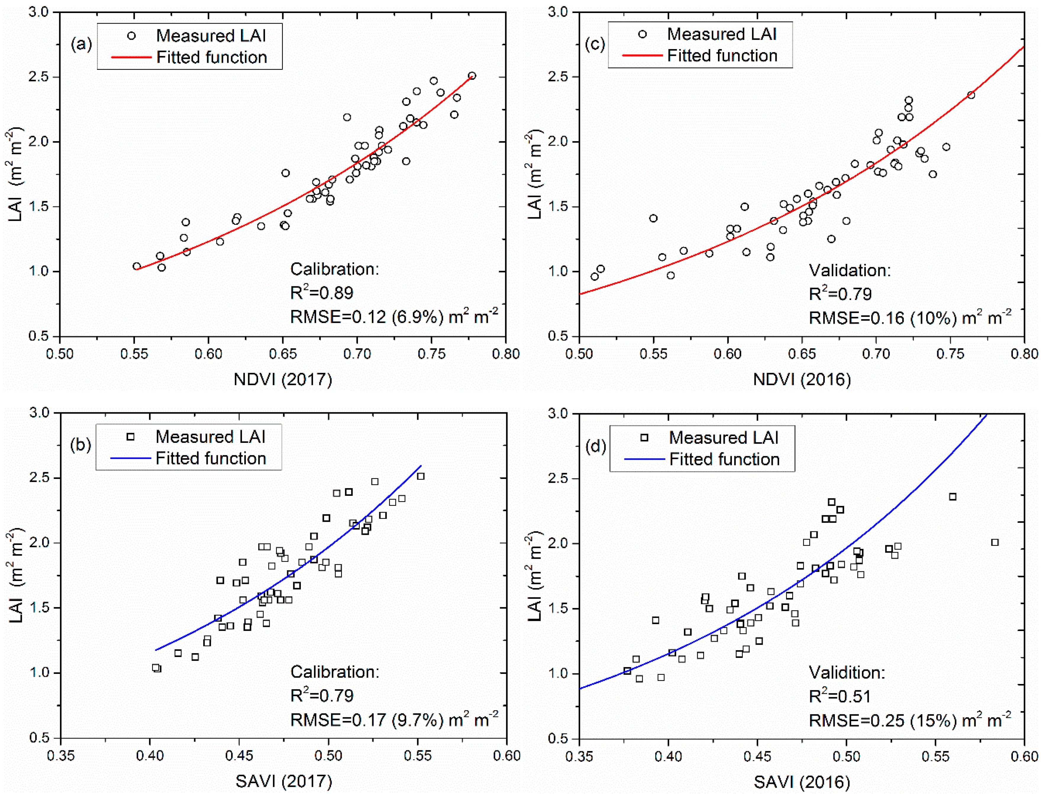
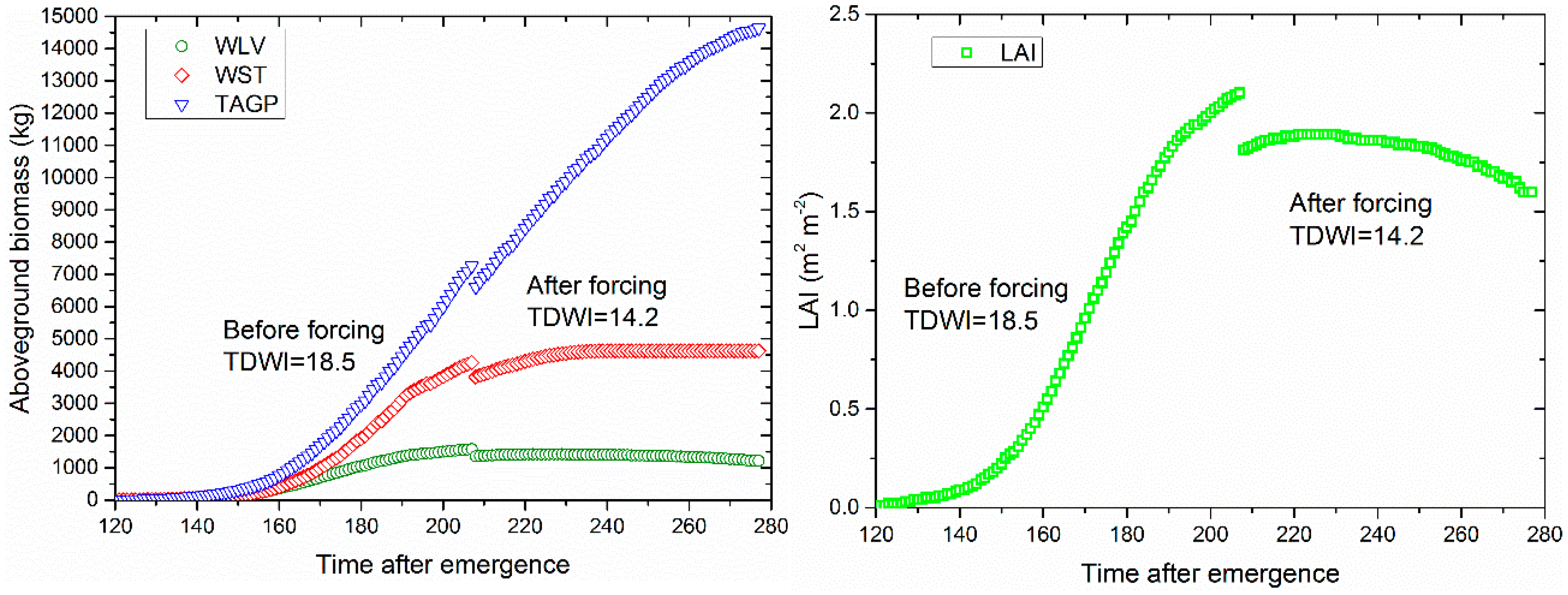
• Yield estimation after forcing LAI: A statistical regression model between LAI and the remotely-sensed vegetation index was firstly established for LAI estimation of 181 samples. Then, a single LAI (near to maximum LAI stages) derived from Landsat data was forced into the calibrated WOFOST model to re-calculate TDWIs, thereby re-driving the model for yield prediction. The yield of 181 samples was re-estimated.
• Accuracy evaluation: In addition to comparing the yield prediction accuracy of the above three methods, the TDWI values of 55 sampled orchards obtained from the assimilation method were also verified and evaluated.

2.3. Description of the WOFOST Model

The WOFOST model was chosen for this study because the model can achieve the quantitative analysis of the growth and production for crops [3]. In addition, in our previous work, the WOFOST model had been evaluated to have the potential to simulate jujube growth and predict yield [66]. It is a mechanistic model that explains crop growth on the basis of the underlying processes, such as phenological development, CO₂-assimilation, transpiration, respiration, and how these processes are influenced by environmental conditions [4]. However, the size of the area where WOFOST can be applied is limited because the crop model’s nonlinear response to the input causes the aggregation effect [66]. In practice, the limitation is resolved by splitting the model spatial domain into small spatial units where the model inputs can be assumed constant. WOFOST includes three operating modes: potential growth, limited growth, and reduced growth. In this study, a potential production pattern was adopted and water stress was not considered because local rainfall was less and jujube water requirements were largely dependent on precision irrigation. LAI is one of the most important state variables in the WOFOST model because it represents the ability of crops to absorb solar radiation, which drives CO₂ assimilation and is a key indicator of crop yield. Three depths in the canopy are selected according to the Gaussian integration method and at those levels the leaf area index, the amount of absorbed radiation, and the leaf CO₂ assimilation are calculated. The total instantaneous assimilation is easily obtained by multiplying the instantaneous assimilation with the total leaf area index [4].

The leaf area index of the three depths can be calculated by using Equation (1):

$$LA{I}_L=\left(0.5+P\sqrt{0.15}\right)LAI\hspace{1em}P=-1, 0, 1$$

(1)

where $LA{I}_L$: Leaf area index at relative distance L in the canopy (ha ha⁻¹)

The light absorbed at a certain depth in the canopy is obtained by Equation (2) with respect to the cumulative leaf area index:

$$I_{a, L}=k\left(1-\rho \right)I_0{e}^{-kLA{I}_L}$$

(2)

where

• I_a: Amount absorbed of specified radiation flux (J m⁻² s⁻¹).
• I_a,L: Amount absorbed of total radiation flux at relative depth L (J m⁻² s⁻¹).
• I₀: Photosynthetically active radiation flux at top of the canopy (J m⁻² s⁻¹).
• k: The extinction coefficient for the PAR flux.
• ρ: Reflection coefficient of the canopy.

The CO₂ assimilation rate can be obtained by introducing the absorbed amount of light into an assimilation-light response function of individual leaves, see Equation (3):

$$A_L=A_m\left(1-e^{\frac{-\epsilon I_a}{A_m}}\right)$$

(3)

where

• A_L: Gross assimilation rate at relative depth L (per unit leaf area) (kg ha⁻¹ h⁻¹).
• A_m: Gross assimilation rate at light saturation (kg ha⁻¹ h⁻¹).
• ε: Initial light use efficiency (kg ha⁻¹ h⁻¹)/(J m⁻¹ s⁻¹).

The total assimilation rate for the whole canopy can be calculated by multiplying the weighted average of the total instantaneous assimilation rates by LAI, see Equation (4):

$$A_C=A_{C,t}\times LAI=\frac{\left(A_{T,L,-1}+1.6A_{T,L,0}+A_{T,L,1}\right)}{3.6}\times LAI$$

(4)

where

• A_C: Total gross assimilation rate for the whole canopy (kg ha⁻¹ h⁻¹).
• A_C,t: Total gross canopy assimilation rate per unit leaf area (kg ha⁻¹ h⁻¹).
• A_T,L,P: Total instantaneous gross assimilation rate at relative depth L (kg ha⁻¹ h⁻¹).
• LAI: Total leaf area of the crop (ha ha⁻¹).

2.4. Study Data

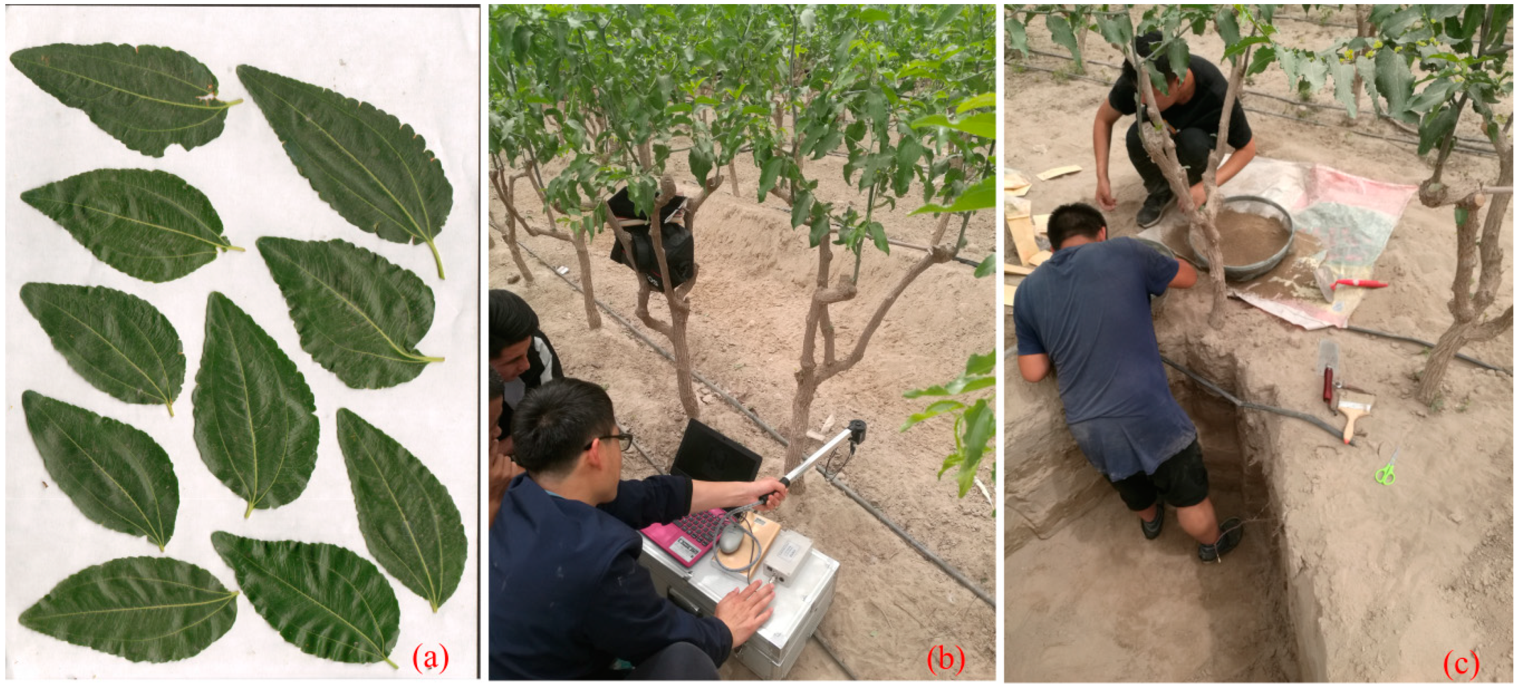
2.4.1. Field Experimental Data for WOFOST Calibration and Validation

In order to calibrate the WOFOST model for our research use, field experiments were conducted in two jujube orchards located in the district of Alaer in Xinjiang, China, during the growing seasons of 2016–2018 (81°13′2″E, 40°34′45″N) (Figure 1, red circle). For crop parameters correction (CV. Jun jujube), emergence, flowering, and maturity dates were recorded. Stems, leaves, fruit dry weight, and LAI were measured ten times each year. LAI in the experimental area were measured using scanning method. First, the collected leaves were tiled onto A4 white paper, then the scanner was used to obtain the tiff format image file and, finally, the leaf area index was calculated using the LA-S Plant canopy analysis system software (WSeen, Hangzhou, China). Figure 2a showed a set of scanned leaves. CO₂ assimilation parameters were obtained from a fitted light response curve based on a rectangular hyperbolic correction model [67]. The net photosynthetic rate was measured with a LI-COR 6400XT portable photosynthesis system (LI-COR, Lincoln, United States). For weather data, daily maximum and minimum temperatures, solar radiation, wind speed at 2 m high, actual vapor pressure, and precipitation were observed using an automatic weather station 500 m from the field experiment. For soil parameters, field capacity, saturated soil moisture content, soil moisture content at wilting point, bulk density, hydraulic conductivity, and water retention parameters were measured before emergence. The depth and weight of the root were sampled by digging a profile (Figure 2c) and measured in the lab.

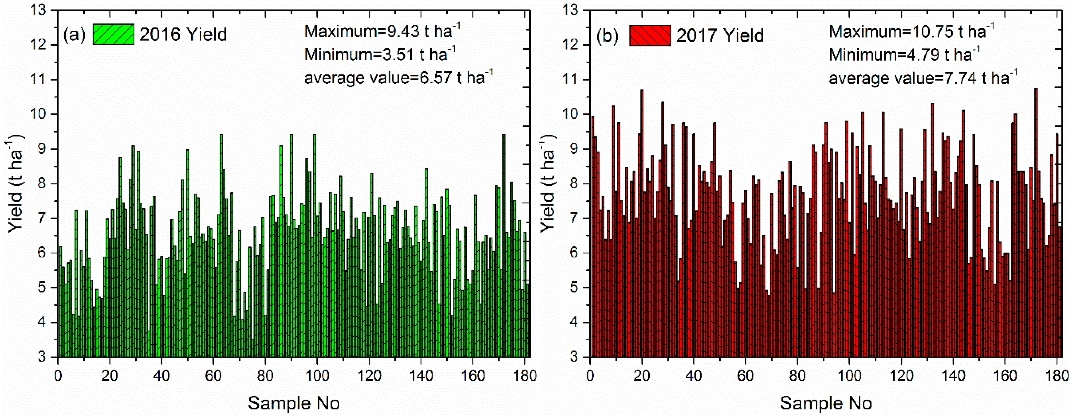
2.4.2. Field-Scale Observation Data for Different Orchards

(1) Yield data for 181 samples

In order to verify the yield prediction performance of the proposed method, the yield data of 181 samples were manually measured after harvesting at the beginning of November, see Figure 3. A small canopy permanent line tree shape was carried out for all sampled orchards to reduce the impact of pruning on research results. All 181 samples accounted for 18,823 pixels in the Landsat satellite imagery. The smallest and largest orchards accounted for 45 and 210 pixels, respectively, with an average of 104. Jujube trees were planted from 2007–2014, including the variability of tree age. The average yield in 2017 was higher than 2016.

(2) TDWI and LAI data for 55 samples

It is difficult to measure TDWIs and LAIs of all 181 samples on the day of the satellite coverage study area. In order to meet the requirements of timeliness, 55 in situ orchards from 181 yield observations in 2016 and 2017 were chosen to measure two key parameters, including TDWI at the true emergence and LAI near to the max vegetative development stages when the Landsat 8 satellite covered the study area. For LAI measurement, each sample plot consisted of four relatively homogeneous subplots (30 m × 30 m) [31]. LAI was measured for six 5 m × 5 m areas uniformly distributed within each subplot by using a fruit tree canopy analyzer (TOP-1300, Zhejiang Top Cloud-agri Technology Co., Ltd., China) calibrated by scanning method (Figure 2b). Average LAI values from the four subplots were calculated to represent the unique LAI value in each sample plot. LAI values measured on 24 July 2016 and 27 July 2017 were used in this study because these two days were the time for the Landsat 8 satellite to cover the study area and near to maximum LAI development stages. The center and edge positions of each sample spot were recorded using the Global Positioning System so that it could be georeferenced to the Landsat 8 remote sensing images. TDWI at emergence was redefined as the weight of the initial new organs (initial buds and roots). The time when the fifth leaf on the bud was unfolded was defined as the time of emergence. The total buds weight for an orchard was calculated by multiplying measuring average buds weight of a tree by the planting density. Then, TDWI values for different orchards were calculated by measuring the dry weight of buds at each orchard and distribution coefficient from field experiment (default value: 70% for buds).

2.5. Calibration of WOFOST Model

The parameters for WOFOST model were calibrated based on collecting data from field detailed experiments. The calibrated parameters were from five sources: measured value, estimated value based on observed data, calibrated value based on measured data, default value from the WOFOST model, fine-tuning values around the default data from the WOFOST model. The calibrated detail and parameters can be found in a previous report from the research team [66]. The phenological development stages, time series of TAGP and LAI were employed to evaluate the calibrated accuracy.

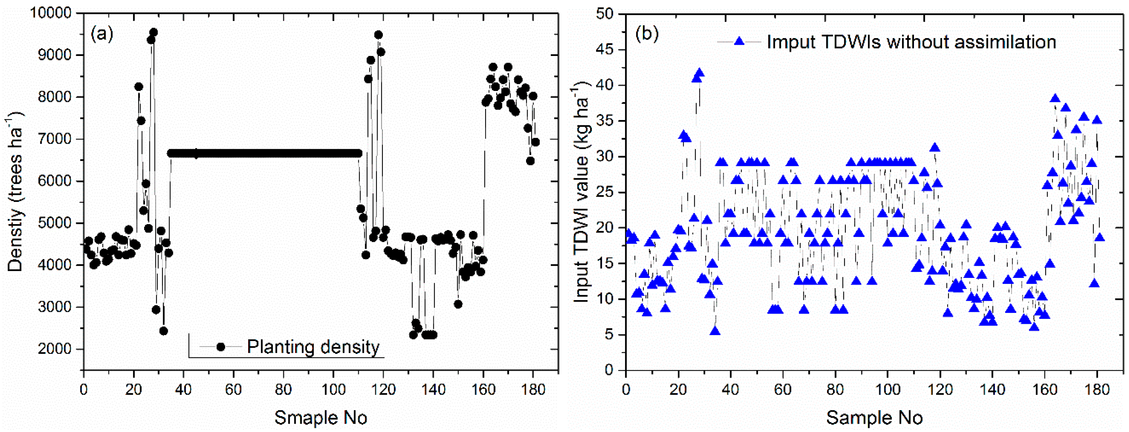
2.6. Input TDWIs for WOFOST Model without Forcing LAI and Yield Estimation

Weather, calibrated jujube data from the field experiment, and soil data were first input into WOFOST model. Based on experimental observations, the TDWI value of each orchard was mainly affected by tree age and planting density. The average TDWI of each tree gradually increased with the increase of the age of the tree, and remained basically unchanged when the tree age is greater than 10. The average TDWI per tree for 3–10 years old was 4.88, 6.24, 9.24, 13.17, 14.28, 16.31, 19.73, and 21.61 g, respectively, based on the measured TDWI values of 148 trees. Planting densities for 181 samples are shown in Figure 4a. The input TDWI values without forcing were calculated using the planting density of each orchard multiplied by the average TDWI per tree with the same tree age (Figure 4b), which were input into the calibrated WOFOST model to respectively simulate the yield for 181 orchards.

2.7. Yield Estimation Using Remotely-Sensed Vegetation Index Regression Method

In each growing season, cloud-free Landsat 8 satellite data during the main growth season were acquired from the USGS (https://earthexplorer.usgs.gov/) (four images for 2016 and six images for 2017). Landsat 8 carried two sensors, the Operational Land Imager (OLI) and the Thermal Infrared Sensor (TIRS). The two sensors can coincidently collect multispectral digital images of the global land surface. Band 4 (red) and 5 (near-infrared) were used in this study for vegetation index extraction. First, the geometric correction was carried out based on the Albers conical equal-area map projection using 50 field-measured ground control points, including road intersection, important building and farmland intersection. The root-mean-square error (RMSE) of the corrected and measured locations was less than one pixel (30 m) for each TM image. Second, the Fast Line-of-sight Atmospheric Analysis of Spectral Hypercubus (FLAASH) model was applied for an atmospheric correction [68]. Third, a border file for Alaer City was used to extract our study area. Finally, NDVI [69] and SAVI [70] for all samples were calculated by Equations (5) and (6), respectively:

$$\mathrm{NDVI}=\frac{{\rho }_{nir}-{\rho }_{red}}{{\rho }_{nir}+{\rho }_{red}}$$

(5)

$$\mathrm{SAVI}=\frac{{\rho }_{nir}-{\rho }_{red}}{{\rho }_{nir}+{\rho }_{red}+L}\times \left(1+L\right)\hspace{1em}\hspace{1em}L=0.5$$

(6)

where ${\rho }_{nir}$ and ${\rho }_{red}$ are the spectral reflectance from the NIR-band (fifth band) and RED-band (fourth band) of Landsat 8 images, respectively.

Firstly, correlations between NDVI, SAVI obtained from Landsat 8 during the main growth season and yields of 181 samples were compared for the best modelling time and vegetation indices (VIs). In addition, the yield prediction performance of max VI, average VI of July and August, average VI from 15 July to 15 August were also tested to expect to get a fit VI. Secondly, the accuracy of four fitted equations between yield and the best VI, including linear, exponential, power and logarithmic models, were compared to determine the equation with highest performance. Finally, data from 181 in situ samples from 2016 and 2017 were used to cross-validate the prediction accuracy for remotely sensed VI regression method.

2.8. Forcing Remotely Sensed LAI and Yield Estimation

Based on 55 observations for LAI, the accuracy of the LAI regression model for 2016 and 2017 was cross-validated. The results showed that the accuracy of the LAI prediction model established using 2017 data was slightly higher than 2016. Therefore, the fitted equation between NDVIs or SAVIs and LAIs was established based on observations from 27 July 2017, and data from 24 July 2016 was used to validate the performance for LAI inversion. The validated VI-LAI model was employed to estimate LAI values for 181 samples. Since heading LAI played the dominant role in improving assimilation accuracy compared with LAI during other phenological stages [31], LAI derived from Landsat 8 data at a near peak vegetative stages (24 July 2016 and 27 July 2017) was forced into the calibrated WOFOST model to re-correct the TDWI value of each sample using the Shuffled Complex Evolution (SCE) optimization algorithm [43]. The cost function was usually set to the sum of the squares or absolute value of the errors between the observed and simulated LAI when multi-temporal observed LAIs were assimilated into the crop growth model [43,46]. In this research, only a single LAI was used in the assimilation, so the cost function (Equation (7)) was constructed as the difference between the simulated and observed values of LAI [46] in order to improve computational efficiency. The SCE was thought to be successful when the cost function was approximately equal to zero:

$$J_{LAI}=LA{I}_{obs}-LA{I}_{sim}$$

(7)

where $J_{LAI}$ was the value of the cost function, $LA{I}_{obs}$ was the value of remotely sensed LAI, $LA{I}_{sim}$ was the value of simulated LAI. The re-correct TDWI value was employed to re-drive the model for yield prediction. The corrected value of the state variable, here LAI, determined the growth rate of the state variables at next time step. Therefore, it was assumed that the final simulated yield was close to the actual value [52].

2.9. Accuracy Evaluation

Coefficient of determination (R²) was used to evaluate the agreement between predicted or simulated values and measured values, see Equation (8). The root mean square error (RMSE) and a normalized root mean square error (NRMSE) were employed to quantify the prediction accuracy, see Equations (9) and (10). The relative bias error (RBE, %) and the % mean absolute error (MAE, %) were also used to evaluate prediction performance, which were shown in Equations (11) and (12), respectively:

$$R^2=1-\frac{{{\displaystyle \sum }}_{i=1}^n{\left(y_i-{\tilde{y}}_i\right)}^2}{{{\displaystyle \sum }}_{i=1}^n{\left(y_i-{\overline{y}}_i\right)}^2}$$

(8)

$$RMSE=\sqrt{\frac{{{\displaystyle \sum }}_{i=1}^n{\left({\tilde{y}}_i-y_i\right)}^2}{n}}$$

(9)

$$NRMSE=\frac{\sqrt{\frac{{{\displaystyle \sum }}_{i=1}^n{\left({\tilde{y}}_i-y_i\right)}^2}{n}}}{{\overline{y}}_{i }}$$

(10)

$$RBE(\%)=\frac{{\tilde{y}}_i-y_i}{y_i}$$

(11)

$$MAE(\%)=\frac{{{\displaystyle \sum }}_{i=1}^n\left|{\tilde{y}}_i-y_i\right|}{n\times {\overline{y}}_{i }}$$

(12)

where ${\tilde{y}}_i$ was the predicted or simulated values, $y_i$ was the observed or measured values, ${\overline{y}}_i$ was the mean of the observed or measured values, and $n$ was the number of samples.

3. Results

3.1. Yield Estimation Using the Remote Sensing Regression Method

Average correlations for two years between a single VI during the main period and yields are shown in Figure 5. The peak correlation based on NDVI or SAVI occurred on the 14th half-month, showing a max value of 0.84 for NDVI, 0.77 for SAVI, respectively. The days were in the main fruit filling period and also close to the maximum vegetative development stages. The results also showed that the average correlation between NDVI and yield was higher than that of SAVI, with a 10% and 3% improvement of 14th and 15th half-months. Therefore, NDVI was employed to establish prediction model for yield. The yield data of 181 in situ samples in two years were also used to cross-validate the prediction accuracy.

Table 1. The comparison of yield prediction performance for several NDVIs.

Index Based on NDVI	Year	Cross-validation (2016 versus 2017)
		R2	NRMSE (%)
14th half-month	2016	0.25	16
	2017	0.33	14.3
Max	2016	0.1	17.5
	2017	0.24	15.3
Average for 7th and 8th month	2016	/	21.3
	2017	/	18.2
Average for 14th and 15th half-month	2016	0.35	14.8
	2017	0.43	13.3

“/” represents that R² is less than zero.

showed a comparison of the yield prediction performance for a single NDVI with highest correlation and composite NDVIs. The average NDVI for 14th and 15th half-months showed better yield prediction ability than single and other composite NDVIs, with a prediction error of 14.8% and 13.3% for 2016 and 2017, followed by NDVI from 14th half-month. Cross-validation prediction equations based on two years of yield data are shown in Equations (13) and (14):

$$2016 \mathrm{validation}:\mathit{yield}=1.01914\times e^{3.06548\times \mathit{NDVI}}$$

(13)

$$2017 \mathrm{validation}:\mathit{yield}=0.77227\times e^{3.33227\times \mathit{NDVI}}$$

(14)

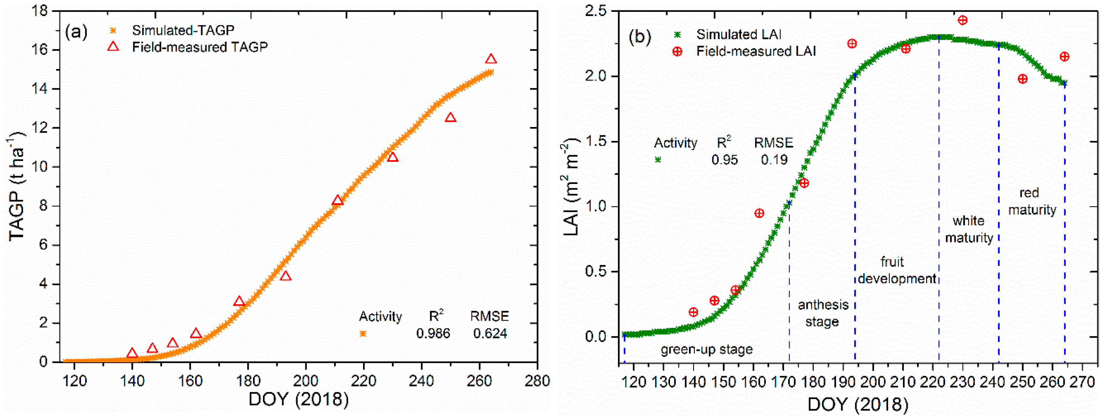
3.2. Calibration of the WOFOST Model

The calibrated main parameters for WOFOST model are shown in

Table 2. Calibrated main model parameters.

Parameter	Description	Value	Units	Source
*Emergence
TBASEM	Lower threshold temperature emergence	10	°C	e
TEFFMX	Max effective temperature emergence	30	°C	e
TSUMEM	Temperature sum from sowing to emergence	230	°C	m-c
*Phenology
TSUM1	Temperature sum from emergence to anthesis	967	°C d−1	m-c
TSUM2	Temperature sum from anthesis to maturity	960	°C d−1	m-c
DTSMTB0	Daily increase in temperature sum as function of at average = 0 °C	0.00	°C d−1	e
DTSMTB100	Daily increase in temperature sum as function of at average = 10 °C	0.00	°C d−1	e
DTSMTB355	Daily increase in temperature sum as function of at average = 35.5 °C	25.5	°C d−1	e
DTSMTB400	Daily increase in temperature sum as function of at average = 40 °C	25.5	°C d−1	e
*Initial parameters
TDWI	Redefine initial total emergence dry weight	/	kg ha−1	m
LAIEM	Leaf area index at emergence	0.0007	ha ha−1	d
RGRLAI	Maximum relative increase in LAI	0.05	ha ha−1 d−1	d
*Green area
SLATB000	Specific leaf area while DVS = 0	0.00165	ha kg−1	m-c
SLATB55	Specific leaf area while DVS = 0.55	0.0013	ha kg−1	m-c
SLATB100	Specific leaf area while DVS = 1	0.0013	ha kg−1	m-c
SLATB200	Specific leaf area while DVS = 2	0.0014	ha kg−1	m-c
SPAN	Life span of leaves growing at 35 °C	60	[d]	e
TBASE	Lower threshold temp. for ageing of leaves	10	°C	e
*CO2 assimilation
KDIFTB00	Extinction coefficient for diffuse visible light at DVS = 0	0.8	\	m-c
KDIFTB200	Extinction coefficient for diffuse visible light at DVS = 2	0.8	\	m-c
EFFTB19.5	Light-use efficiency single leaf at average temp. = Celsius	0.495	kg ha−1 hr−1J−1 m2 s	m-c
EFFTB355	Light-use efficiency single leaf at average temp. = Celsius	0.495	kg ha−1 hr−1J−1 m2 s	m-c
AMAXTB00	Maximum leaf CO2 assimilation. Rate at DVS = 0	39.0	kg ha−1 hr−1	m-c
AMAXTB170	Maximum leaf CO2 assimilation. Rate at DVS = 1.7	39.0	kg ha−1 hr−1	m-c
AMAXTB200	Maximum leaf CO2 assimilation. Rate at DVS = 2	20.0	kg ha−1 hr−1	m-c
TMPFTB10	Reduction factor of AMAX of at 10 ℃	0	\	d
TMPFTB195	Reduction factor of AMAX of at 19.5 ℃	1	\	d
TMPFTB355	Reduction factor of AMAX of at 35.5 ℃	1	\	d
*Conversion of assimilates into biomass
CVL	Efficiency of conversion into leaves	0.732	kg kg−1	m-c
CVO	Efficiency of conversion into storage organs	0.780	kg kg−1	m-c
CVR	Efficiency of conversion into roots	0.690	kg kg−1	m-c
CVS	Efficiency of conversion into stems	0.751	kg kg−1	m-c
*maintenance respiration
Q10	Relative increase in respiration rate per 10 °C temperature increase	2	kg CH2O kg−1 d−1	d
RML	Relative maintenance respiration rate of leaves	0.03	kg CH2O kg−1 d−1	d
RMO	Relative maintenance respiration rate of storage organs	0.01	kg CH2O kg−1 d−1	d-c
RMR	Relative maintenance respiration rate of roots	0.01	kg CH2O kg−1 d−1	d
RMS	Relative maintenance respiration rate of stems	0.015	kg CH2O kg−1 d−1	d-c
*Partitioning parameters
FRTB00	Fraction of above-ground dry matter to roots at DVS = 0	0.3	kg kg−1	m-c
FRTB154	Fraction of above-ground dry matter to roots at DVS = 1.54	0.0	kg kg−1	m-c
FLTB00	Fraction of above-ground dry matter to leaves at DVS = 0	0.67	kg kg−1	m-c
FLTB012	Fraction of above-ground dry matter to leaves at DVS = 0.12	0.31	kg kg−1	m-c
FLTB022	Fraction of above-ground dry matter to leaves at DVS = 0.22	0.41	kg kg−1	m-c
FLTB032	Fraction of above-ground dry matter to leaves at DVS = 0.32	0.55	kg kg−1	m-c
FLTB051	Fraction of above-ground dry matter to leaves at DVS = 0.51	0.4	kg kg−1	m-c
FLTB097	Fraction of above-ground dry matter to leaves at DVS = 0.97	0.15	kg kg−1	m-c
FLTB100	Fraction of above-ground dry matter to leaves at DVS = 1.00	0.1	kg kg−1	m-c
FSTB00	Fraction of above-ground dry matter to stems at DVS = 0	0.33	kg kg−1	m-c
FSTB012	Fraction of above-ground dry matter to stems at DVS = 0.12	0.69	kg kg−1	m-c
FSTB022	Fraction of above-ground dry matter to stems at DVS = 0.22	0.59	kg kg−1	m-c
FSTB032	Fraction of above-ground dry matter to stems at DVS = 0.32	0.45	kg kg−1	m-c
FSTB051	Fraction of above-ground dry matter to stems at DVS = 0.51	0.6	kg kg−1	m-c
FSTB097	Fraction of above-ground dry matter to stems at DVS = 0.97	0.85	kg kg−1	m-c
FSTB100	Fraction of above-ground dry matter to stems at DVS = 1.00	0.43	kg kg−1	m-c
FSTB145	Fraction of above-ground dry matter to stems at DVS = 1.45	0.2	kg kg−1	m-c
FOTB100	Fraction of above-ground dry matter to storage organs at DVS = 1.00	0.47	kg kg−1	m-c
FOTB145	Fraction of above-ground dry matter to storage organs at DVS = 1.45	0.8	kg kg−1	m-c
FOTB164	Fraction of above-ground dry matter to storage organs at DVS = 1.64	1.0	kg kg−1	m-c
FOTB200	Fraction of above-ground dry matter to storage organs at DVS = 2.00	1	kg kg−1	m-c
*Death rates
RDRSTB00	Relative death rate of stems at DVS = 0	0	\	e
RDRSTB200	Relative death rate of stems at DVS = 2.0	0	\	e

d, default; e, estimated; m, measured; m–c, calibrated on the basis of the measured data; d–c, fine tuning around default data. TDWIs for different orchards were re-calibrated by using forcing LAI.

. The phenological development time was firstly calibrated based on effective accumulated temperature, with a validated error of −2, −3, and −3 days for emergence, flowering and maturity, respectively. The simulated total aboveground biomass (TAGP) and leaf area index (LAI) agreed well with the field-measured values, showing a validated R² of 0.986 (Figure 6a) and 0.95 (Figure 6b), respectively. The prediction errors (RMSE) were 0.624 t ha⁻¹ and 0.19 m² m⁻², respectively. Yield and total biomass differences between simulated and observed were found to be 4.8% and 4%, respectively.

TDWI strongly influences the initial growth rate and represents an obvious uncertainty in the WOFOST model [4]. The trajectory of the effect of TDWI on simulated LAI during the growing season and yield is shown in Figure 7. The simulated maximum LAI and yield showed an increasing trend with the increase of TDWI, and the ratio of the increase was gradually decreasing. However, when the simulated LAI was above a certain threshold, the simulated yield will decrease. Since the excessive LAI will cause the light energy at the bottom of the canopy to be intercepted, the photosynthesis efficiency will decrease. Therefore, TDWI was considered as a significant correction parameter while running the model on field-scale orchards with different planting densities and tree ages.

3.3. Remotely-Sensed LAI

The results of the calibrated versus validated LAI based on NDVI and SAVI are shown in Figure 8. In the calibration or validation sets, the LAI regression results using NDVI were higher than using SAVI. Calibrated R² and RMSE were 0.89 and 0.12 (6.9%) m² m⁻² for NDVI, 0.79 and 0.17 (9.7%) m² m⁻² for SAVI, respectively, and the validated R² and RMSE were 0.79 and 0.16 (10%) m² m⁻² for NDVI, 0.51 and 0.25 (15%) m² m⁻² for SAVI, respectively. Previous studies had also confirmed that NDVI may perform better LAI prediction accuracy than SAVI when vegetation coverage was high [31]. The best regression equation for LAI and NDVI is shown in Equation (15):

$$LAI=0.1115\times e^{4.00316\times NDVI}$$

(15)

3.4. Forcing Remotely-Sensed LAI and Yield Estimation

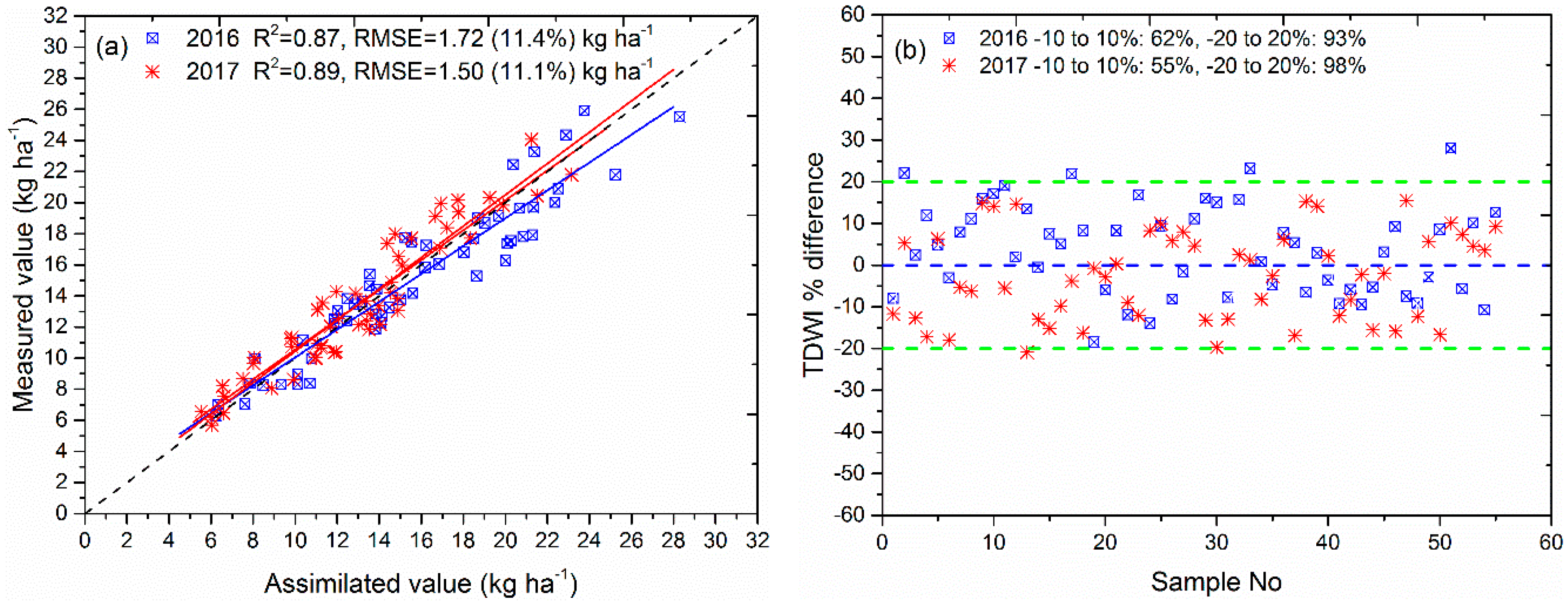
3.4.1. Re-Calibrated TDWI Evaluation after Forcing LAI

Based on TDWI data from 55 samples, the scatterplot of the re-calibrated TDWI after forcing LAI versus measured values is shown in Figure 9a. Agreement metrics demonstrated the calibrated values were well agreed with measured value (R² = 0.87 and R² = 0.89, respectively). The predicted RMSE (NRMSE) were 1.72 (11.4%) and 1.50 (11.1%) kg ha⁻¹ for 2016 and 2017, respectively. The percentage difference of more than half of the samples was between −10% and 10%, with 62% for 2016 and 55% for 2017 (Figure 9b). 93% and 98% of the samples had only a predicted deviation between −20% and 20% for 2016 and 2017, respectively.

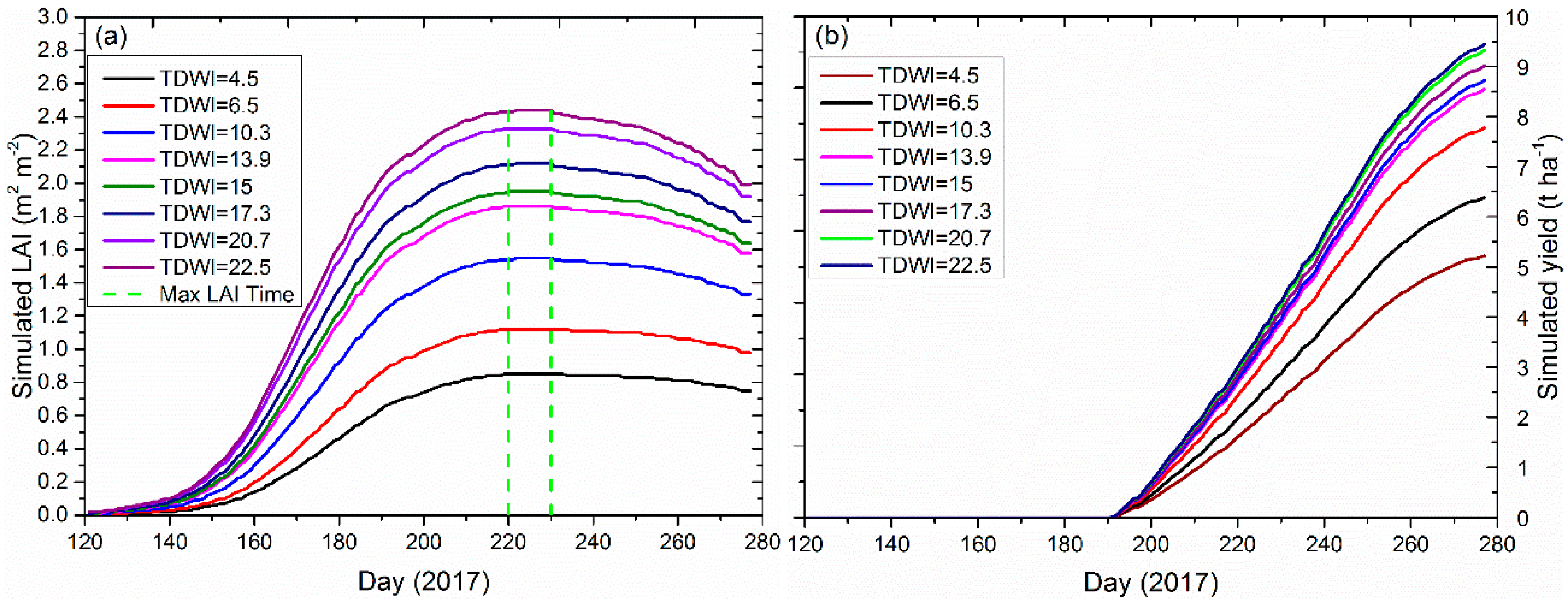
3.4.2. Aboveground Biomass Simulation after Forcing LAI

Taking the third sample as an example, the simulated dry weight of leaves, stems and total above-ground biomass before and after forcing LAI are shown in Figure 10. The values of all growth parameters after forcing became lower than their respective values before forcing. The total aboveground biomass and LAI were reduced from 7255 to 6606 kg ha⁻¹ and 2.1 to 1.81 m² m⁻² at forcing time, respectively. The input TDWI was designed as a default value (see Figure 4b) before assimilation, which was significantly higher than the actual measured value of 13.8 kg ha⁻¹. Therefore, the actual yield and LAI were also overestimated. However, the forced TDWI value had a smaller deviation from the actual value. With these corrections in modelled growth parameters after assimilation, the actual yield per orchard was re-estimated.

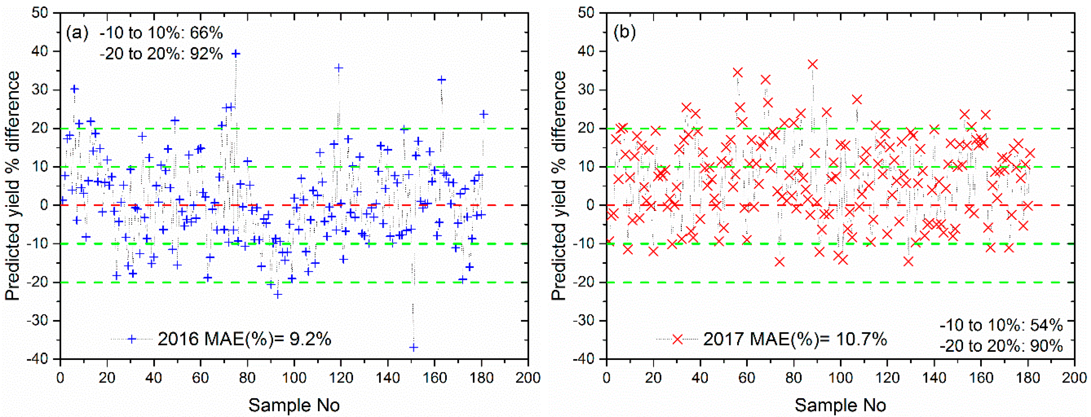
3.4.3. Yield Estimation after Forcing LAI

For forcing method, the % mean absolute error (MAE, %) of simulated yields versus measured values was 9.2% and 10.7% for 2016 and 2017, respectively (Figure 11). The relative % difference (RBE, %) of more than half of the samples was between −10% and 10% (66% for 2016 and 54% for 2017). More than 90% of the samples showed a predicted deviation between −20% and 20%, with values of 92% and 90% for 2016 and 2017, respectively.

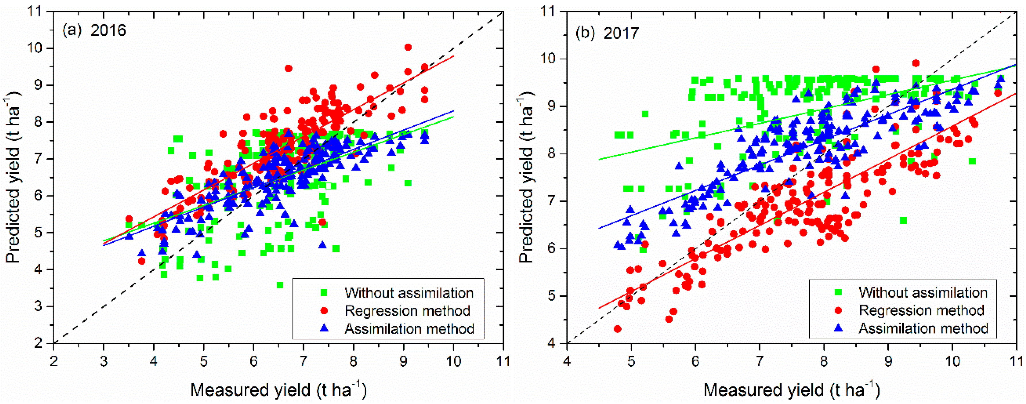
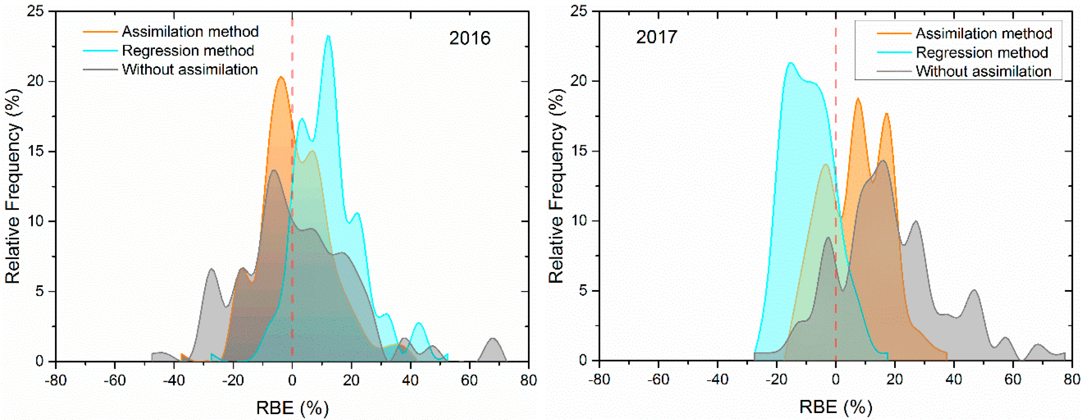
3.5. Comparison of Three Prediction Methods

The scatterplots of the three yield prediction methods, including without assimilation, assimilation and remote sensing regression methods, versus measured values are shown in Figure 12. The simulated yield without forcing LAI was discrete and clearly deviating from the actual value. The results also indicated that there was still a high error for setting the default TDWI value for the same aged jujube orchards. The simulation performance of the model was significantly improved while the LAI near to the maximum vegetative development stages was forced into the calibrated WOFOST model. The remote sensing regression method also showed better ability than the without assimilation method. However, for the assimilation methods, actual yields were overestimated and underestimated at low yields and high yields, respectively. The reason may be that the CO₂ assimilation rate increased with the increase of tree age, and this factor was not considered in this study, which led to the overestimation of the yield at low tree age and underestimation at high tree age.

Figure 13 shows the distributions of RBE (%) values for three prediction methods. The assimilation method resulted in relative bias errors that were distributed more centrally around zero compared with the simulation without assimilation and the remote sensing regression method. The absolute RBE for yield simulation was lower than 15% in 80% and 72% of the samples, lower than 20% in 92% and 90% for 2016 and 2017, respectively. The results also indicated the better performance of the assimilation-based estimation to reproduce the spatial distribution for jujube yields although five and three samples were overestimated and underestimated more than 30% in 2016 and 2017, respectively. The reason may be that simulation results were affected by unconsidered factors of the model, such as pruning and pests and disease protection.

The positive results achieved by assimilation method were also confirmed by the indices of agreement and error between simulated and observed yields (

Table 3. Accuracy comparison of three prediction methods.

Prediction Method	Year	R2	RMSE (%) t ha−1	MAE (%)
Without assimilation	2016	0.09	1.16 (17.6)	14.9
	2017	0.13	1.67 (21.5)	20.3
Remotely sensed average NDVI prediction (cross-validation)	2016	0.35	0.98 (14.8)	13.3
	2017	0.43	1.02 (13.3)	14.9
Forcing LAI (assimilation)	2016	0.62	0.74 (10.9)	9.2
	2017	0.59	0.87 (11.1)	10.7

a. Numbers in brackets are percentages of RMSE to average actual yields

). The assimilation method showed the highest performance, with a R² of 0.62 and RMSE of 0.74 (10.9%) t ha⁻¹ for 2016, and a R² of 0.59 and RMSE of 0.87 (11.1%) t ha⁻¹ for 2017, followed by the remotely-sensed NDVI regression method (R² = 0.35, RMSE = 0.98 (14.8%) t ha⁻¹ for 2016 and R² = 0.43, RMSE = 1.02 (13.3%) t ha⁻¹ for 2017), and finally without assimilation (R² = 0.09, RMSE = 1.16 (17.6%) t ha⁻¹ for 2016 and R² = 0.13, RMSE = 1.67 (21.5%) t ha⁻¹ for 2017). The best MAE values were also achieved by assimilation method, showing an improvement of 31% and 28% versus the remote sensing regression method, and 38% and 47% versus the simulation without assimilation in 2016 and 2017, respectively.

4. Discussion

Previous studies have reported the use of remote sensing (Landsat 7 and 8) vegetation indices to predict fruit crop yields at field scale, showing low relative errors from 6.9% to 11.5% for grape yield prediction [71]. Rahman et al. [72] also explored the potential of WorldView-3 imagery for predicting the yield of mango, showing a R² value ranging from 0.79–0.93 and RMSE from 7.9–9.1 kg tree⁻¹ for three orchards. However, phenology information should be considered when performing crop yield predictions, and a time series of VI shall be useful for crop yield forecasting [73]. In this research, the predicted yield based on the remotely-sensed NDVI was overestimated in 2016 and was underestimated in 2017 (Figure 12, red circle). The reason may be that the length of the 2016 growing season is about 12 days lower than in 2017. However, the effect of phenological length on yield is not considered when the cross-validation based on the remote sensing regression method is performed. In addition, although remote sensing satellites with medium and high spatial resolution have the potential to be used for field-scale yield prediction, it is a challenge to construct a time series of vegetation indices for consideration of phenological information due to low temporal resolution. In contrast, crop growth model can takes into account the growth process of the phenology. However, for the prediction method using the WOFOST model, the predicted yields of most samples are overestimated in 2017. The main reason may be that uncertainty in strongly varying tree age and planting densities may be introduced into the model structure, which may lead to a simulated yield bias for different orchards. For the assimilation method, the TDWI parameter is considered for responding to uncertainty in tree age and planting density for fruit tree crops in this research. An approach forcing the LAI near the peak vegetative stage into a calibrated WOFOST model was attempted to reduce the uncertainty and simulate the yield for a perennial jujube fruit tree crop at the field-scale, showing a well performance (MAE = 9.2% and 10.7% for 2016 and 2017, respectively). However, actual yields are slightly overestimated and underestimated at low yields and high yields in 2016 and 2017, respectively. Two reasons may cause this deviation. The first reason may be that the CO₂ assimilation rate increased with the increase of tree age, and the CO₂ assimilation parameters are set to fixed values in this research, which can lead to overestimation of yield at low tree age and underestimation at high tree age. The second reason may be the genetic varieties of phenological stages and crop characteristics, such as special leaf area (SLATB) and CO₂ assimilation parameters, thereby influencing potential yield. These parameters are expected to be further optimized by assimilation of remote sensing information.

Previous studies have proved that the heading LAI plays a key role in improving assimilation accuracy compared with LAI during other phenological stages [31,52]. In addition, jujube yield is highly correlated with the maximum LAI [74]. In our study, a single LAI near to the maximum LAI stages was also proven to have potential for assimilation to improve yield prediction accuracy. However, a forced method was used in our study, and the assimilation accuracy mainly relied on the accuracy of the state variables obtained by remote sensing. For TM satellite data with a resolution of 30 m, mixed pixels are inevitably present in the process of inverting LAI and predicting yields. In particular, the pixels may be mixed with shelter forests and roads at the edge of the orchard, resulting in a decrease in the accuracy of the observed LAI. There errors from remote sensing observation data may be introduced into crop models when the assimilation is completed. Remote sensing data with higher spatial resolution can provide high-precision state variable estimation and can be recommended for inverting state variables to improve the accuracy of the observed variables. In addition, the combination of higher spatial resolution satellite data and TM satellite data is also expected to improve LAI inversion accuracy and yield prediction capabilities. Although the calibration and updating methods with greater flexibility can minimize the simulation error and the remote sensing inversion error, it requires sufficient observation spots [12]. High spatial resolution satellites typically have low temporal resolution and are often challenging to obtain more efficient observations. Therefore, fully exploiting the potential of a single observational data is valuable for remote sensing assimilation of fruit tree crops planted in a specific region.

In this study, LAI was assimilated into the crop model as the only state variable. Although LAI is an important indicator for canopy light interception and CO₂ assimilation, a single LAI does not accurately express the effect of effective radiation, temperature, nitrogen, and soil moisture content on jujube yield [31]. LAI, biomass, leaf nitrogen accumulation, evapotranspiration, and soil moisture obtained from remote sensing data can be expected to assimilate into calibrated WOFOST model to optimize state variables and improve simulated accuracy for jujube yield. In addition, the WOFOST model is carried out with a potential production simulation. The effects of other factors such as water stress have not been considered. Temporal evolution of LAI and final yields can change with irrigation management and soil properties in different regions. The state variable SM (soil moisture content) can be recommended to respond to water transport conditions in rain-fed or irrigated jujube gardens when the model is carried out in a moisture-limited production simulation [3]. Moreover, differences in plant diseases and pests, nitrogen stress, and jujube genetic parameters are not considered in the study. These several limiting factors can occur in the field, so that the external conditions are beyond the boundary conditions of the effective model range and influence the yield prediction accuracy while carrying out data assimilation [12]. How to respond to these factors in the model will also be a valuable research exploration. Furthermore, the same pruning structure, a small canopy permanent line tree shape, was performed in all sampled orchards to avoid the effect of pruning on the simulation results. For fruit tree crops, an extension of the analysis whether the proposed approach is suitable for jujube orchards with different tree shapes is also needed to be further validated.

5. Conclusions

In this study, the WOFOST process-based growth model was tried to estimate the jujube tree yield at a field scale. The modelling accuracy was enhanced by incorporating a single remotely-sensed LAI near to the max vegetative development periods from Landsat 8 data into the WOFOST model. Research results indicated the recalibrated TDWI by forcing LAI can response to tree age and planting density on yield and represents higher prediction accuracy. The proposed method is a promising way for the use of long-revisit cycle and medium spatial resolution remote sensing satellites for assimilation research. This study can provide an approach that improves fruit tree crop yield estimation at field scale. Note that the proposed method shows a slight deviation in high-yield and low-yield orchards because the effect of tree age on CO₂ assimilation parameters and specific leaf parameters is not considered. In addition, when the model is applied to orchards with different pruning trees, the CO₂ assimilation parameters may also need to be re-corrected. In future research work, the following two research contents can be highlighted:

• Remotely-sensed state variable SM can be recommended to be assimilated into the WOFOST model in response to the effects of irrigation and rainfall on the simulation results.
• The influence of tree age and shapes on CO₂ assimilation parameters and the use of remote sensing data to optimize these parameters are also worth exploring in order to improve simulation accuracy in high-yield and low-yield jujube gardens.

References

1. Ouédraogo, S.J.; Bayala, J.; Dembélé, C.; Kaboré, A.; Kaya, B.; Niang, A.; Somé, A.N. Establishing jujube trees in sub-Saharan Africa: Response of introduced and local cultivars to rock phosphate and water supply in Burkina Faso, West Africa. Agrofor. Syst. 2006, 68, 69–80. [Google Scholar] [CrossRef]
2. Lam, C.T.W.; Chan, P.H.; Lee, P.S.C.; Lau, K.M.; Kong, A.Y.Y.; Gong, A.G.W.; Xu, M.L.; Lam, K.Y.C.; Dong, T.T.X.; Lin, H.; et al. Chemical and biological assessment of Jujube (Ziziphus jujuba)-containing herbal decoctions: Induction of erythropoietin expression in cultures. J. Chromatogr. B Anal. Technol. Biomed. Life Sci. 2015, 1026, 254–262. [Google Scholar] [CrossRef]
3. de Wit, A.; Boogaard, H.; Fumagalli, D.; Janssen, S.; Knapen, R.; van Kraalingen, D.; Supit, I.; van der Wijngaart, R.; van Diepen, K. 25 years of the WOFOST cropping systems model. Agric. Syst. 2019, 168, 154–167. [Google Scholar] [CrossRef]
4. van Diepen, C.A.; Wolf, J.; van Keulen, H.; Rappoldt, C. WOFOST: A simulation model of crop production. Soil Use Manag. 1989, 5, 16–24. [Google Scholar] [CrossRef]
5. Jones, J.W.; Hoogenboom, G.; Porter, C.H.; Boote, K.J.; Batchelor, W.D.; Hunt, L.A.; Wilkens, P.W.; Singh, U.; Gijsman, A.J.; Ritchie, J.T. The DSSAT cropping system model. Eur. J. Agron. 2003, 18, 235–265. [Google Scholar] [CrossRef]
6. Wang, X.; Williams, J.R.; Gassman, P.W.; Baffaut, C.; Izaurralde, R.C.; Jeong, J.; Kiniry, J.R. EPIC and APEX: Model Use, Calibration, and Validation. Trans. ASABE 2012, 55, 1447–1462. [Google Scholar] [CrossRef]
7. Brisson, N.; Gary, C.; Justes, E.; Roche, R.; Mary, B.; Ripoche, D.; Zimmer, D.; Sierra, J.; Bertuzzi, P.; Burger, P.; et al. An overview of the crop model STICS. Eur. J. Agron. 2003, 18, 309–332. [Google Scholar] [CrossRef]
8. Holzworth, D.P.; Huth, N.I.; deVoil, P.G.; Zurcher, E.J.; Herrmann, N.I.; McLean, G.; Chenu, K.; van Oosterom, E.J.; Snow, V.; Murphy, C.; et al. APSIM—Evolution towards a new generation of agricultural systems simulation. Environ. Model. Softw. 2014, 62, 327–350. [Google Scholar] [CrossRef]
9. Van Dam, J.C.; Wesseling, J.G.; Feddes, R.A.; Kabat, P.; Van Walsum, P.E.V.; Van Diepen, C.A. Theory of SWAP version 2.0. Softw. Man. 1997, 153. Available online: https://library.wur.nl/WebQuery/wurpubs/fulltext/222782 (accessed on 1April 2019).
10. Raes, D.; Steduto, P.; Hsiao, T.C.; Fereres, E. Aquacrop-The FAO crop model to simulate yield response to water: II. main algorithms and software description. Agron. J. 2009, 101, 438–447. [Google Scholar] [CrossRef]
11. Stöckle, C.O.; Donatelli, M.; Nelson, R. CropSyst, a cropping systems simulation model. Eur. J. Agron. 2003, 18, 289–307. [Google Scholar] [CrossRef]
12. Jin, X.; Kumar, L.; Li, Z.; Feng, H.; Xu, X.; Yang, G.; Wang, J. A review of data assimilation of remote sensing and crop models. Eur. J. Agron. 2018, 92, 141–152. [Google Scholar] [CrossRef]
13. De Wit, A.; Duveiller, G.; Defourny, P. Estimating regional winter wheat yield with WOFOST through the assimilation of green area index retrieved from MODIS observations. Agric. For. Meteorol. 2012, 164, 39–52. [Google Scholar] [CrossRef]
14. Fang, H.; Liang, S.; Hoogenboom, G.; Teasdale, J.; Cavigelli, M. Corn-yield estimation through assimilation of remotely sensed data into the CSM-CERES-Maize model. Int. J. Remote Sens. 2008, 29, 3011–3032. [Google Scholar] [CrossRef]
15. Jiang, Z.; Chen, Z.; Chen, J.; Liu, J.; Ren, J.; Li, Z.; Sun, L.; Li, H. Application of Crop Model Data Assimilation With a Particle Filter for Estimating Regional Winter Wheat Yields. IEEE J. Sel. Top. Appl. Earth Obs. Remote Sens. 2014, 7, 4422–4431. [Google Scholar] [CrossRef]
16. Nearing, G.S.; Crow, W.T.; Thorp, K.R.; Moran, M.S.; Reichle, R.H.; Gupta, H. Assimilating remote sensing observations of leaf area index and soil moisture for wheat yield estimates: An observing system simulation experiment. Water Resour. Res. 2012, 48. [Google Scholar] [CrossRef]
17. Yao, F.; Tang, Y.; Wang, P.; Zhang, J. Estimation of maize yield by using a process-based model and remote sensing data in the Northeast China Plain. Phys. Chem. Earth 2015, 87–88, 142–152. [Google Scholar] [CrossRef]
18. Jin, X.; Yang, G.; Xu, X.; Yang, H.; Feng, H.; Li, Z.; Shen, J.; Lan, Y.; Zhao, C. Combined multi-temporal optical and radar parameters for estimating LAI and biomass in winter wheat using HJ and RADARSAR-2 data. Remote Sens. 2015, 7, 13251–13272. [Google Scholar] [CrossRef]
19. Huang, Y.; Zhu, Y.; Li, W.; Cao, W.; Tian, Y. Assimilating Remotely Sensed Information with the WheatGrow Model Based on the Ensemble Square Root Filter for Improving Regional Wheat Yield Forecasts. Plant Prod. Sci. 2013, 16, 352–364. [Google Scholar] [CrossRef]
20. Bastiaanssen, W.G.; Ali, S. A new crop yield forecasting model based on satellite measurements applied across the Indus Basin, Pakistan. Agric. Ecosyst. Environ. 2003, 94, 321–340. [Google Scholar] [CrossRef]
21. Huang, J.; Ma, H.; Su, W.; Zhang, X.; Huang, Y.; Fan, J. Jointly Assimilating MODIS LAI and ET Products Into the SWAP Model for Winter Wheat Yield Estimation. IEEE J. Sel. Top. Appl. Earth Obs. Remote Sens. 2015, 8, 4060–4071. [Google Scholar] [CrossRef]
22. Dente, L.; Satalino, G.; Mattia, F.; Rinaldi, M. Assimilation of leaf area index derived from ASAR and MERIS data into CERES-Wheat model to map wheat yield. Remote Sens. Environ. 2008, 112, 1395–1407. [Google Scholar] [CrossRef]
23. Ines, A.V.M.; Das, N.N.; Hansen, J.W.; Njoku, E.G. Assimilation of remotely sensed soil moisture and vegetation with a crop simulation model for maize yield prediction. Remote Sens. Environ. 2013, 138, 149–164. [Google Scholar] [CrossRef]
24. Chakrabarti, S.; Bongiovanni, T.; Judge, J.; Zotarelli, L.; Bayer, C. Assimilation of SMOS soil moisture for quantifying drought impacts on crop yield in agricultural regions. IEEE J. Sel. Top. Appl. Earth Obs. Remote Sens. 2014, 7, 3867–3879. [Google Scholar] [CrossRef]
25. Sakamoto, T.; Yokozawa, M.; Toritani, H.; Shibayama, M.; Ishitsuka, N.; Ohno, H. A crop phenology detection method using time-series MODIS data. Remote Sens. Environ. 2005, 96, 366–374. [Google Scholar] [CrossRef]
26. Delécolle, R.; Maas, S.J.; Guérif, M.; Baret, F. Remote sensing and crop production models: Present trends. ISPRS J. Photogramm. Remote Sens. 1992, 47, 145–161. [Google Scholar] [CrossRef]
27. Singh, R.; de Wit, A.J.W.; Zurita-Milla, R.; Brazile, J.; Schaepman, M.E.; Dorigo, W.A. A review on reflective remote sensing and data assimilation techniques for enhanced agroecosystem modeling. Int. J. Appl. Earth Obs. Geoinf. 2006, 9, 165–193. [Google Scholar]
28. Argent, R. Land Surface Observation, Modeling and Data Assimilation. Environ. Model. Softw. 2014, 57, 248–249. [Google Scholar] [CrossRef]
29. Moulin, S.; Bondeau, A.; Delécolle, R. Combining agricultural crop models and satellite observations: From field to regional scales. Int. J. Remote Sens. 1998, 19, 1021–1036. [Google Scholar] [CrossRef]
30. Curnel, Y.; de Wit, A.J.W.; Duveiller, G.; Defourny, P. Potential performances of remotely sensed LAI assimilation in WOFOST model based on an OSS Experiment. Agric. For. Meteorol. 2011, 151, 1843–1855. [Google Scholar] [CrossRef]
31. Huang, J.; Tian, L.; Liang, S.; Ma, H.; Becker-Reshef, I.; Huang, Y.; Su, W.; Zhang, X.; Zhu, D.; Wu, W. Improving winter wheat yield estimation by assimilation of the leaf area index from Landsat TM and MODIS data into the WOFOST model. Agric. For. Meteorol. 2015, 204, 106–121. [Google Scholar] [CrossRef]
32. Chen, Y.; Zhang, Z.; Tao, F. Improving regional winter wheat yield estimation through assimilation of phenology and leaf area index from remote sensing data. Eur. J. Agron. 2018, 101, 163–173. [Google Scholar] [CrossRef]
33. Huang, J.; Sedano, F.; Huang, Y.; Ma, H.; Li, X.; Liang, S.; Tian, L.; Zhang, X.; Fan, J.; Wu, W. Assimilating a synthetic Kalman filter leaf area index series into the WOFOST model to improve regional winter wheat yield estimation. Agric. For. Meteorol. 2016, 216, 188–202. [Google Scholar] [CrossRef]
34. Huang, J.; Ma, H.; Sedano, F.; Lewis, P.; Liang, S.; Wu, Q.; Su, W.; Zhang, X.; Zhu, D. Evaluation of regional estimates of winter wheat yield by assimilating three remotely sensed reflectance datasets into the coupled WOFOST–PROSAIL model. Eur. J. Agron. 2019, 102, 1–13. [Google Scholar] [CrossRef]
35. Li, H.; Chen, Z.; Liu, G.; Jiang, Z.; Huang, C. Improving winter wheat yield estimation from the CERES-Wheat model to assimilate leaf area index with different assimilation methods and spatio-temporal scales. Remote Sens. 2017, 9, 190. [Google Scholar] [CrossRef]
36. Guo, C.; Zhang, L.; Zhou, X.; Zhu, Y.; Cao, W.; Qiu, X.; Cheng, T.; Tian, Y. Integrating remote sensing information with crop model to monitor wheat growth and yield based on simulation zone partitioning. Precis. Agric. 2017, 19, 55–78. [Google Scholar] [CrossRef]
37. Xie, Y.; Wang, P.; Bai, X.; Khan, J.; Zhang, S.; Li, L.; Wang, L. Assimilation of the leaf area index and vegetation temperature condition index for winter wheat yield estimation using Landsat imagery and the CERES-Wheat model. Agric. For. Meteorol. 2017, 246, 194–206. [Google Scholar] [CrossRef]
38. Gilardelli, C.; Stella, T.; Confalonieri, R.; Ranghetti, L.; Campos-Taberner, M.; García-Haro, F.J.; Boschetti, M. Downscaling rice yield simulation at sub-field scale using remotely sensed LAI data. Eur. J. Agron. 2019, 103, 108–116. [Google Scholar] [CrossRef]
39. Donohue, R.J.; Lawes, R.A.; Mata, G.; Gobbett, D.; Ouzman, J. Towards a national, remote-sensing-based model for predicting field-scale crop yield. F. Crop. Res. 2018, 227, 79–90. [Google Scholar] [CrossRef]
40. Silvestro, P.C.; Pignatti, S.; Pascucci, S.; Yang, H.; Li, Z.; Yang, G.; Huang, W.; Casa, R. Estimating wheat yield in China at the field and district scale from the assimilation of satellite data into the Aquacrop and simple algorithm for yield (SAFY) models. Remote Sens. 2017, 9, 509. [Google Scholar] [CrossRef]
41. Cheng, Z.; Meng, J.; Wang, Y. Improving spring maize yield estimation at field scale by assimilating time-series HJ-1 CCD data into the WOFOST model using a new method with fast algorithms. Remote Sens. 2016, 8, 303. [Google Scholar] [CrossRef]
42. Jin, X.; Li, Z.; Xu, X.; Yang, G.; Wang, J.; Kumar, L. Estimation of winter wheat biomass and yield by combining the aquacrop model and field hyperspectral data. Remote Sens. 2016, 8, 972. [Google Scholar] [CrossRef]
43. Ma, G.; Huang, J.; Wu, W.; Fan, J.; Zou, J.; Wu, S. Assimilation of MODIS-LAI into the WOFOST model for forecasting regional winter wheat yield. Math. Comput. Model. 2013, 58, 634–643. [Google Scholar] [CrossRef]
44. Zhao, Y.; Chen, S.; Shen, S. Assimilating remote sensing information with crop model using Ensemble Kalman Filter for improving LAI monitoring and yield estimation. Ecol. Modell. 2013, 270, 30–42. [Google Scholar] [CrossRef]
45. Fang, H.; Liang, S.; Hoogenboom, G. Integration of MODIS LAI and vegetation index products with the CSM-CERES-Maize model for corn yield estimation. Int. J. Remote Sens. 2011, 32, 1039–1065. [Google Scholar] [CrossRef]
46. Wang, H.; Zhu, Y.; Li, W.; Cao, W.; Tian, Y. Integrating remotely sensed leaf area index and leaf nitrogen accumulation with RiceGrow model based on particle swarm optimization algorithm for rice grain yield assessment. J. Appl. Remote Sens. 2014, 8. [Google Scholar] [CrossRef]
47. Dong, Y.; Chen, L.; Zhao, C.; Wang, J.; Feng, H.; Yang, G. Integrating a very fast simulated annealing optimization algorithm for crop leaf area index variational assimilation. Math. Comput. Model. 2012, 58, 877–885. [Google Scholar] [CrossRef]
48. Ding, C.; Jiang, J.; Wu, L.; Zhao, L.; Liu, X.; Liu, F. The Dynamic Assessment Model for Monitoring Cadmium Stress Levels in Rice Based on the Assimilation of Remote Sensing and the WOFOST Model. IEEE J. Sel. Top. Appl. Earth Obs. Remote Sens. 2015, 8, 1330–1338. [Google Scholar]
49. Hadria, R.; Duchemin, B.; Lahrouni, A.; Khabba, S.; Er-Raki, S.; Dedieu, G.; Chehbouni, A.G.; Olioso, A. Monitoring of irrigated wheat in a semi-arid climate using crop modelling and remote sensing data: Impact of satellite revisit time frequency. Int. J. Remote Sens. 2006, 27, 1093–1117. [Google Scholar] [CrossRef]
50. Schneider, K. Assimilating remote sensing data into a land-surface process model. Int. J. Remote Sens. 2003, 24, 2959–2980. [Google Scholar] [CrossRef]
51. Thorp, K.R.; Hunsaker, D.J.; French, A.N. Assimilating Leaf Area Index Estimates from Remote Sensing into the Simulations of a Cropping Systems Model. Trans. ASABE. 2013, 53, 251–262. [Google Scholar] [CrossRef]
52. Panigrahy, S.; Mukherjee, J.; Chaudhari, K.N.; Parihar, J.S.; Ray, S.S.; Patel, N.K.; Tripathy, R. Forecasting wheat yield in Punjab state of India by combining crop simulation model WOFOST and remotely sensed inputs. Remote Sens. Lett. 2012, 4, 19–28. [Google Scholar]
53. Jongschaap, R.E.E.; Schouten, L.S.M. Predicting wheat production at regional scale by integration of remote sensing data with a simulation model. Agron. Sustain. Dev. 2005, 25, 481–489. [Google Scholar] [CrossRef]
54. Aubert, D.; Loumagne, C.; Oudin, L. Sequential assimilation of soil moisture and streamflow data in a conceptual rainfall-Runoff model. J. Hydrol. 2003, 280, 145–161. [Google Scholar] [CrossRef]
55. Pellenq, J.; Boulet, G. A methodology to test the pertinence of remote-sensing data assimilation into vegetation models for water and energy exchange at the land surface. Agronomie. 2004, 24, 197–204. [Google Scholar] [CrossRef]
56. Crow, W.T.; Wood, E.F. The assimilation of remotely sensed soil brightness temperature imagery into a land surface model using Ensemble Kalman filtering: A case study based on ESTAR measurements during SGP97. Adv. Water Resour. 2003, 26, 137–149. [Google Scholar] [CrossRef]
57. Lorenc, A.C.; Ballard, S.P.; Bell, R.S.; Ingleby, N.B.; Andrews, P.L.F.; Barker, D.M.; Bray, J.R.; Clayton, A.M.; Dalby, T.; Li, D.; et al. The Met. Office global three-dimensional variational data assimilation scheme. Q. J. R. Meteorol. Soc. 2000, 126, 2991–3012. [Google Scholar] [CrossRef]
58. Trémolet, Y. Model-error estimation in 4D-Var. Q. J. R. Meteorol. Soc. 2007, 133, 1267–1280. [Google Scholar] [CrossRef]
59. Moradkhani, H.; Hsu, K.L.; Gupta, H.; Sorooshian, S. Uncertainty assessment of hydrologic model states and parameters: Sequential data assimilation using the particle filter. Water Resour. Res. 2005, 41, 1–17. [Google Scholar] [CrossRef]
60. Sahu, S.K.; Yip, S.; Holland, D.M. Improved space-time forecasting of next day ozone concentrations in the eastern US. Atmospheric Environ. 2009, 43, 494–501. [Google Scholar] [CrossRef]
61. Plant, N.G.; Holland, K.T. Prediction and assimilation of surf-zone processes using a Bayesian network. Coast. Eng. 2010, 58, 119–130. [Google Scholar] [CrossRef]
62. de Wit, A.J.W.; van Diepen, C.A. Crop model data assimilation with the Ensemble Kalman filter for improving regional crop yield forecasts. Agric. For. Meteorol. 2007, 146, 38–56. [Google Scholar] [CrossRef]
63. Bolten, J.D.; Reynolds, C.A.; Crow, W.T.; Zhan, X.; Jackson, T.J. Evaluating the Utility of Remotely Sensed Soil Moisture Retrievals for Operational Agricultural Drought Monitoring. IEEE J. Sel. Top. Appl. Earth Obs. Remote Sens. 2010, 3, 57–66. [Google Scholar] [CrossRef]
64. Li, Y.; Zhou, Q.; Zhou, J.; Zhang, G.; Chen, C.; Wang, J. Assimilating remote sensing information into a coupled hydrology-crop growth model to estimate regional maize yield in arid regions. Ecol. Model. 2014, 291, 15–27. [Google Scholar] [CrossRef]
65. Bai, T.; Zhang, N.; Chen, Y.; Mercatoris, B. Assessing the Performance of the WOFOST Model in Simulating Jujube Fruit Tree Growth under Different Irrigation Regimes. Sustainability 2019, 11, 1466. [Google Scholar] [CrossRef]
66. Principles of WOFOST (Temporal and Spatial Scale). Available online: https://www.wur.nl/en/Research-Results/Research-Institutes/Environmental-Research/Facilities-Products/Software-and-models/WOFOST/Principles-of-WOFOST.htm (accessed on 1 April 2019).
67. Ye, Z.P.; Yu, Q. Comparison of a New Model of Light Response of Photosynthesis with Traditional Models. J. Shenyang Agric. Univ. 2007, 38, 771–775. (In Chinese) [Google Scholar]
68. RSI. ENVI User’s Guide. September 2001 Edition. 2001. Available online: http://www.harrisgeospatial.com/portals/0/pdfs/envi/ENVI_User_Guide.pdf (accessed on 6 May 2018).
69. Pettorelli, N. The Normalized Difference Vegetation Index. 2013. Available online: https://books.google.be/books?hl=zh-CN&lr=&id=FXywAAAAQBAJ&oi=fnd&pg=PP1&dq=Pettorelli,+N.+The+Normalized+Difference+Vegetation+Index&ots=q1av97XPIL&sig=qsBfWEGJ1SbUqJTaFjGP2qVauww&redir_esc=y#v=onepage&q=Pettorelli%2C%20N.%20The%20Normalized%20Difference%20Vegetation%20Index&f=false (accessed on 15 March 2018).
70. Huete, A. A soil-adjusted vegetation index (SAVI). Remote Sens. Environ. 1988, 25, 295–309. [Google Scholar] [CrossRef]
71. Sun, L.; Gao, F.; Anderson, M.C.; Kustas, W.P.; Alsina, M.M.; Sanchez, L.; Sams, B.; McKee, L.; Dulaney, W.; White, W.A.; et al. Daily mapping of 30 m LAI and NDVI for grape yield prediction in California vineyards. Remote Sens. 2017, 9, 317. [Google Scholar] [CrossRef]
72. Rahman, M.M.; Robson, A.; Bristow, M. Exploring the potential of high resolution worldview-3 Imagery for estimating yield of mango. Remote Sens. 2018, 10, 1866. [Google Scholar] [CrossRef]
73. Bolton, D.K.; Friedl, M.A. Forecasting crop yield using remotely sensed vegetation indices and crop phenology metrics. Agric. For. Meteorol. 2013, 173, 74–84. [Google Scholar] [CrossRef]
74. Yang, W.; Gao, J.; Xu, C.; Wu, C.; Jin, Q. The Correlation Analysis of Leaf Area Index and Yield of Red Jujube. Xinjiang Agric. Sci. 2012, 49, 1397–1400. (In Chinese) [Google Scholar]
Figure 1. Study region and observations. Note: The LAI and TDWI sample set is a subset of yield observations.
Remotesensing 11 01119 g001
Figure 2. (a) A set of leaves scanned for LAI measurement. (b) LAI measurement by using a canopy analyzer. (c) Root depth and weight measurement.
Remotesensing 11 01119 g002
Figure 3. Yields (dry weight) of 181 situ sample spots in 2016 (a) and 2017 (b).
Remotesensing 11 01119 g003
Figure 4. (a) Planting densities for 181 samples. (b) Initial TDWI values without assimilation.
Remotesensing 11 01119 g004
Figure 5. Average correlation coefficient for two years between NDVI (a)/SAVI (b) and yields. Half-month 9 was the first half of May.
Remotesensing 11 01119 g005
Figure 6. (a) Simulated versus measured TAGP. (b) Simulated versus measured LAI.
Remotesensing 11 01119 g006
Figure 7. (a) The change trend of LAI versus TDWI. (b) The change trend of Yield versus TDWI.
Remotesensing 11 01119 g007
Figure 8. Calibrated and validated LAI inversion model (ad) based on NDVI and SAVI.
Remotesensing 11 01119 g008
Figure 9. (a) Re-calibrated TDWI for 2016 and 2017 versus measured value. (b) Percent difference for the re-calibrated TDWI.
Remotesensing 11 01119 g009
Figure 10. Simulated dry weight of leaves (WLV), dry weight of stems (WST), dry weight of total aboveground biomass (TAGP), and LAI before and after forcing.
Remotesensing 11 01119 g010
Figure 11. (a) Relative percentage difference for prediction yields for 2016. (b) Relative percentage difference for prediction yields for 2017.
Remotesensing 11 01119 g011
Figure 12. (a) Predicted versus measured yields based on three methods for 2016. (b) Predicted versus measured yields based on three methods for 2017.
Remotesensing 11 01119 g012
Figure 13. Frequency distributions (%) of relative bias error (RBE; %) resulting from the comparison between observed and simulated yields. RBE % = 0% (red line) represented the perfect prediction. Bin size was equal to 5.
Remotesensing 11 01119 g013