Comparison of Sentinel-2 and High-Resolution Imagery for Mapping Land Abandonment in Fragmented Areas


Abstract
:
1. Introduction
2. Data and Methods
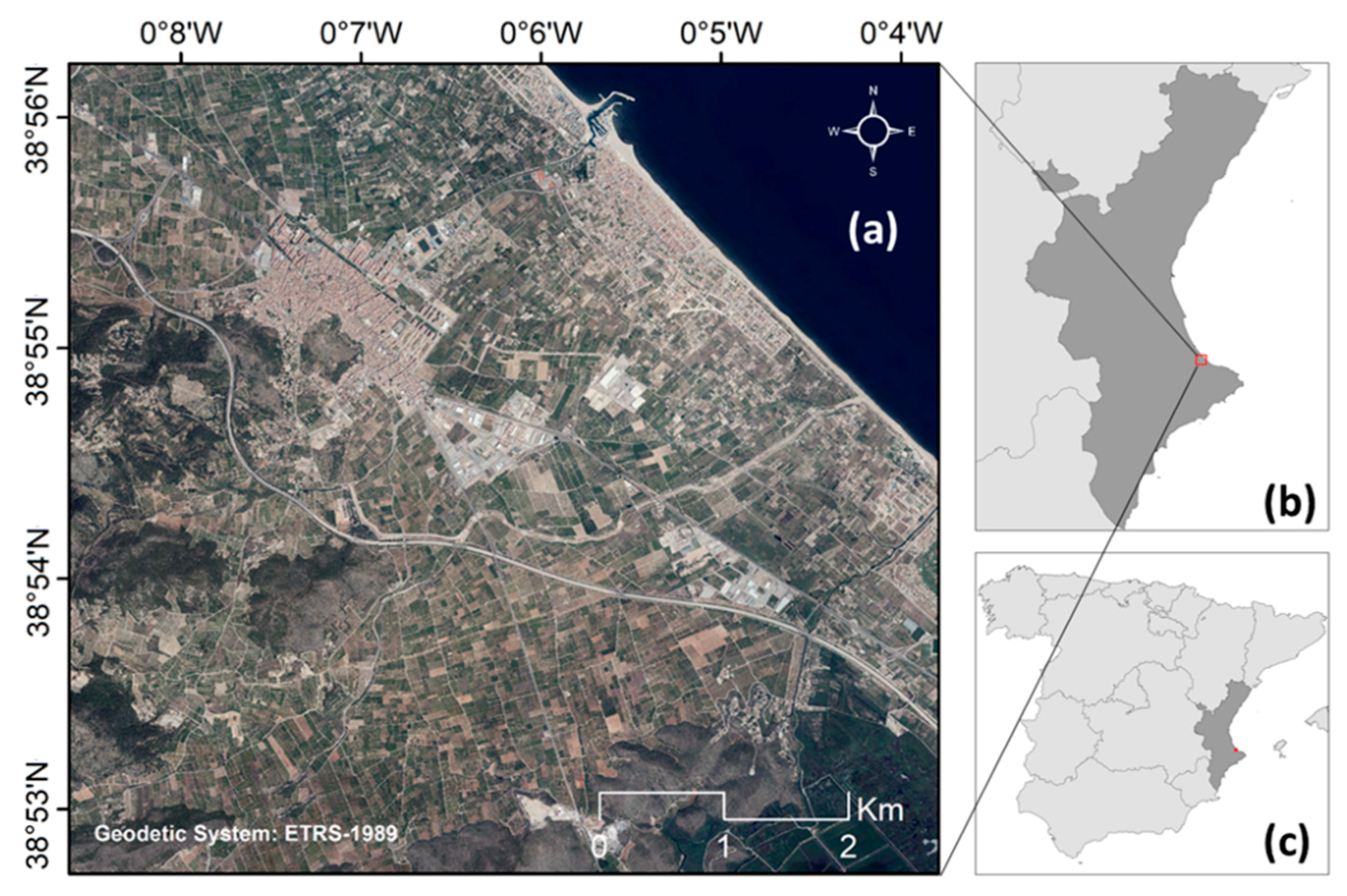
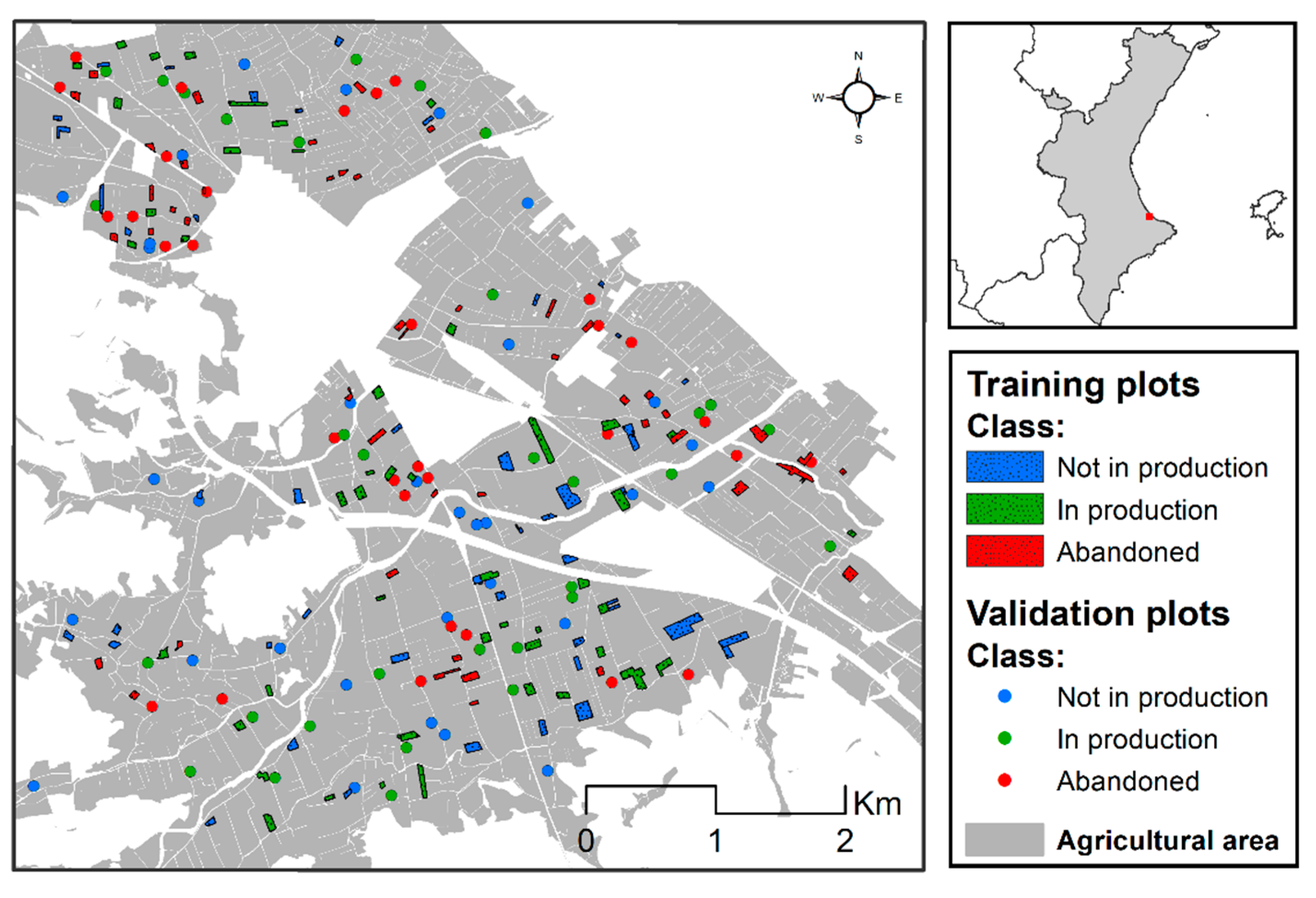
2.1. Study Area
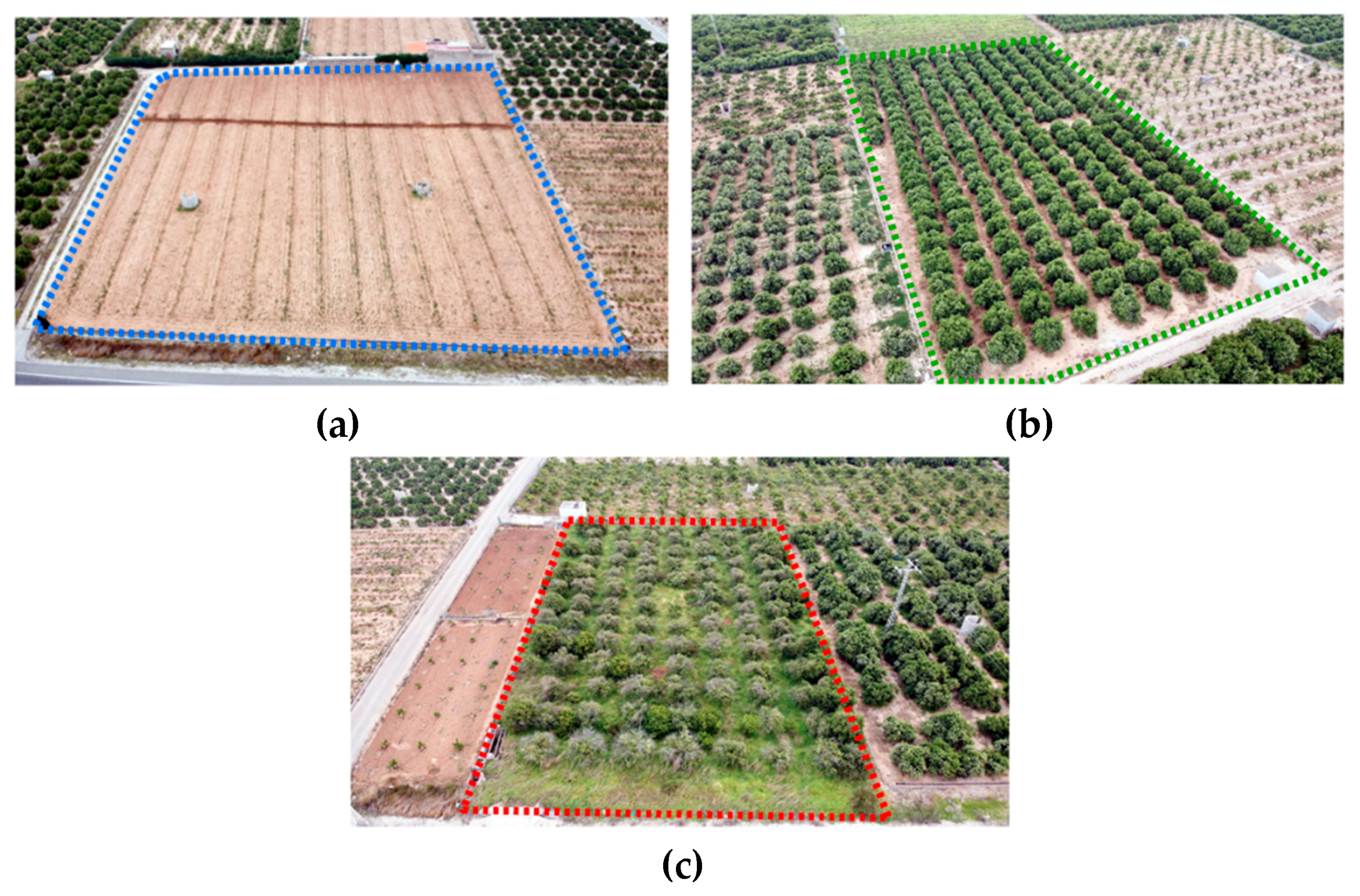
2.2. Land Abandonment Process in Citrus
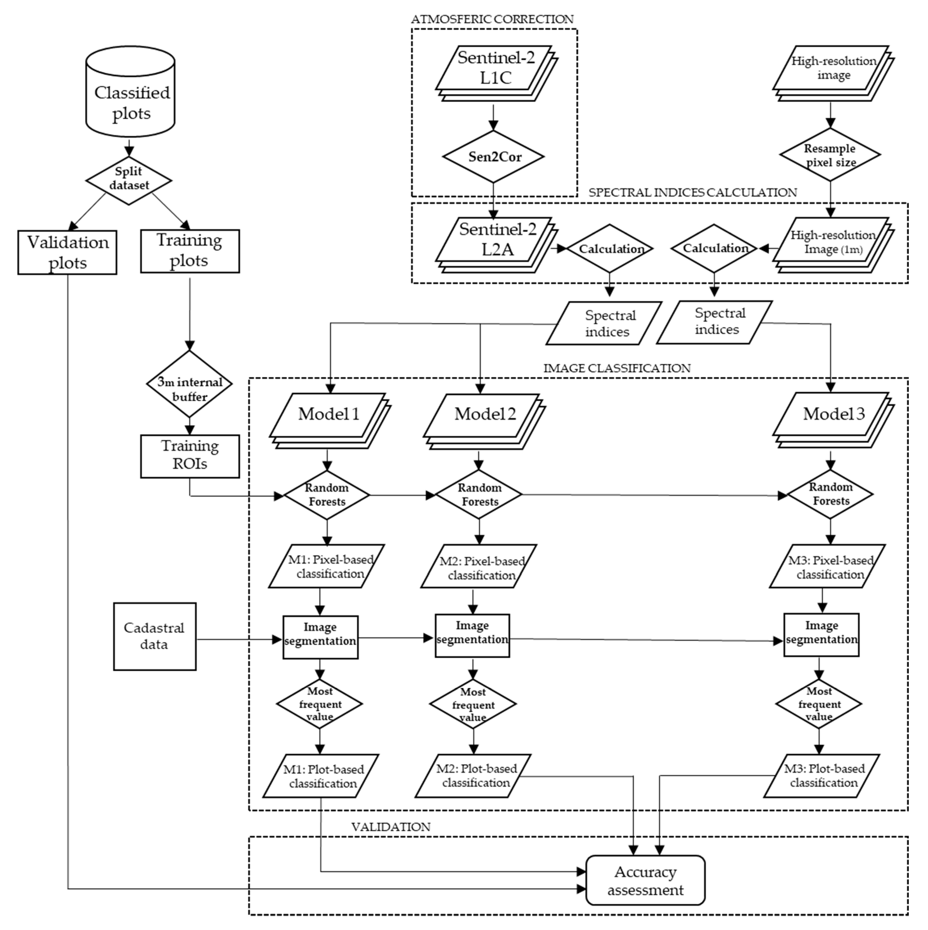
2.3. Data and Processing
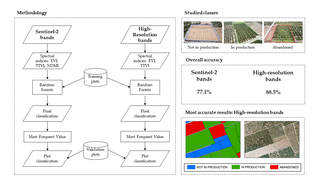
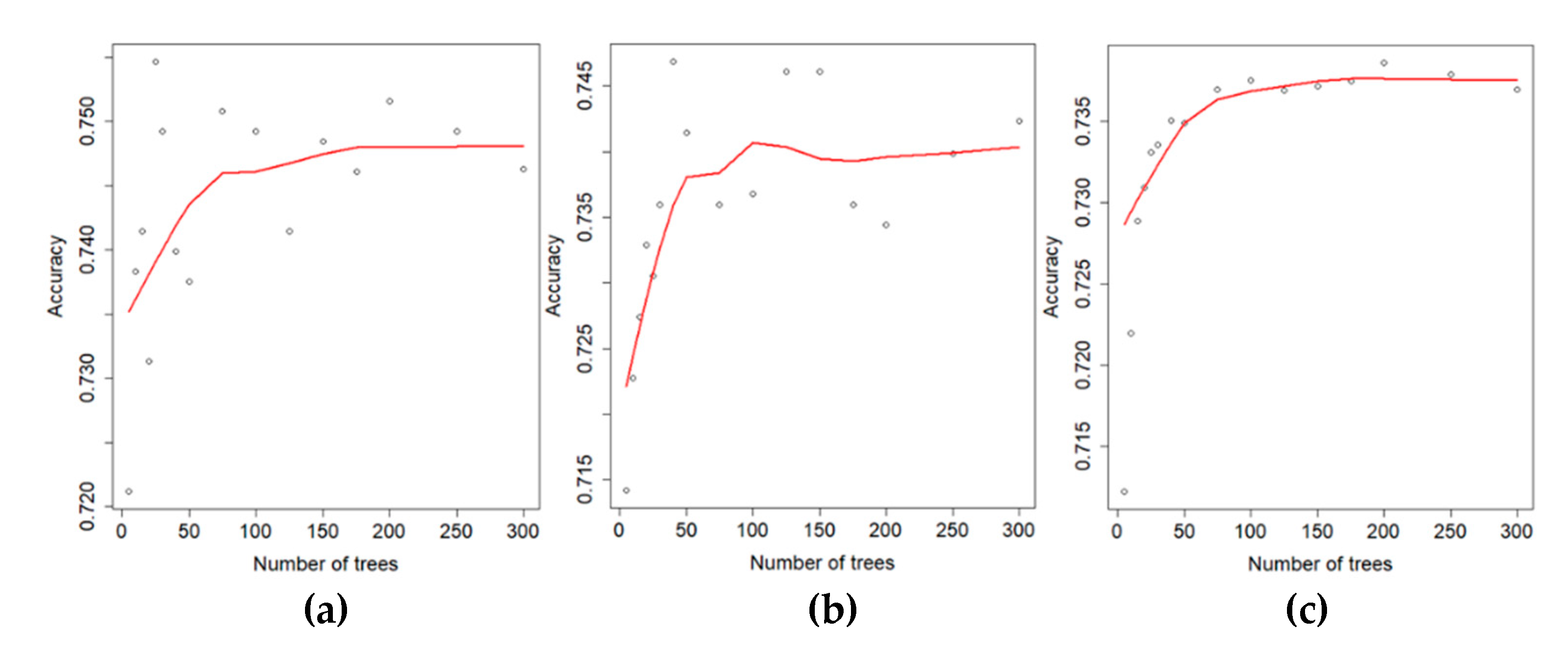
2.4. Classification Algorithm
2.5. Accuracy Assessment and Validation
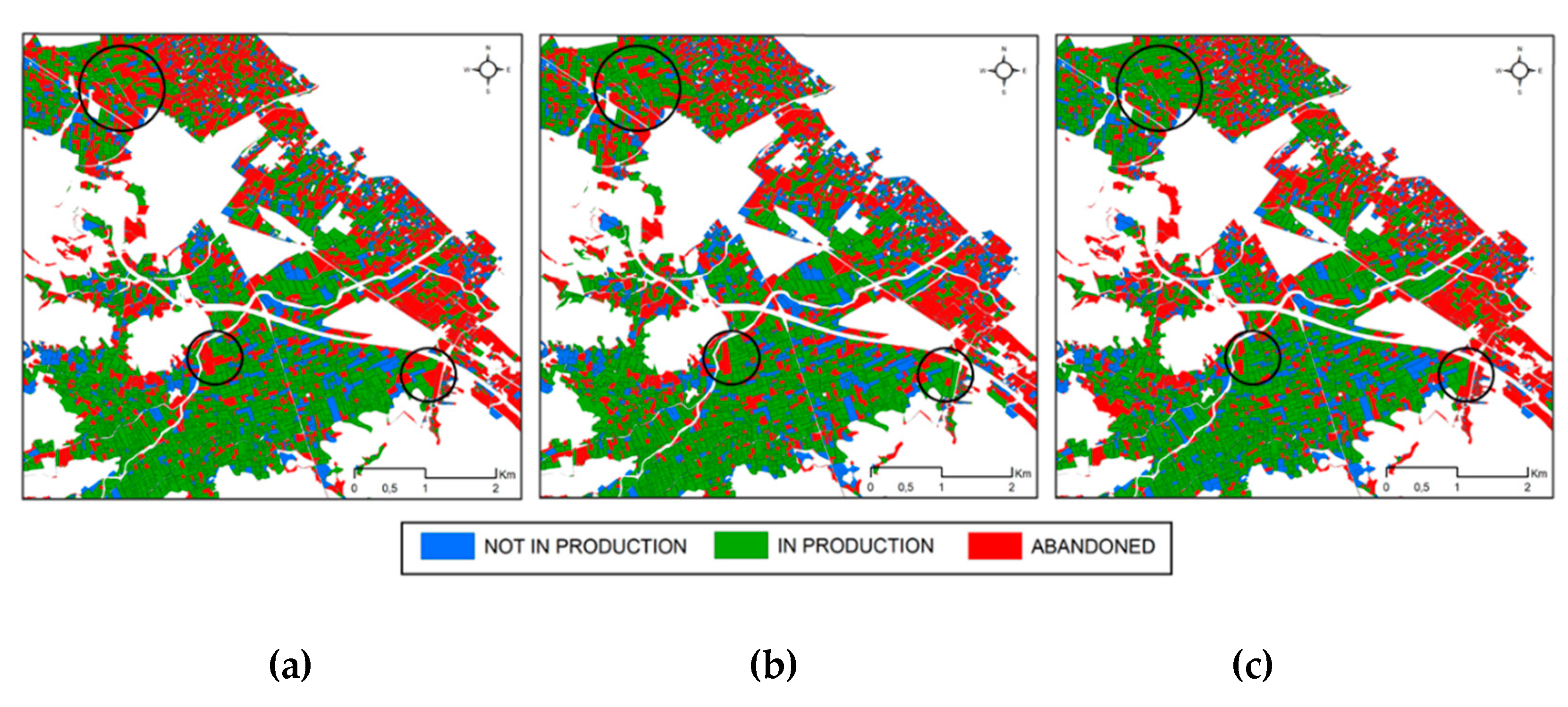
3. Results
4. Discussion
5. Conclusions
Author Contributions
Funding
Conflicts of Interest
References
- MacDonald, D.; Crabtree, J.R.; Wiesinger, T.; Dax, T.; Stamou, N.; Fleury, P.; Lazpita, J.G.; Gibon, A. Agricultural abandonment in mountain areas or Europe: Environmental consequences and policy response. J. Environ. Manag. 2000, 59, 47–69. [Google Scholar] [CrossRef]
- Kosmas, C.; Kairis, O.; Karavitis, C.; Acikalin, S.; Alcalá, M.; Alfama, P.; Atlhopheng, J.; Barrera, J.; Belgacem, A.; Solé-Benet, A.; et al. An exploratory analysis of land abandonment drivers in areas prone to desertification. CATENA 2015, 128, 252–261. [Google Scholar] [CrossRef]
- Corbelle-Rico, E.; Crecente-Maseda, R. Estudio da evolución da superficie agrícola na comarca da Terra Chá a partir de fotografía aérea histórica e mapas de usos, 1956-2004. Recur. Rurais 2018, 4, 57–65. [Google Scholar]
- Baudry, J. Ecological consequences of grazing extensification and land abandonment: Role of interactions between environment, society and techniques. In Land Abandonment and Its Role in Conservation, 1st ed.; Baudry, J., Bunce, R.G.H., Eds.; Options Méditerranéennes: Série A; Séminaires Méditerranéens: Zaragoza, Spain, 1991; Volume 15, pp. 13–19. [Google Scholar]
- Pinto-Correia, T. Land abandonment: Changes in the land use patterns around the Mediterranean basin. Etat de l’Agriculture en Méditerranée. Les sols dans la région méditerranéenne: Utilisation, gestion et perspectives d’évolution. Options Méditerranéennes Série A Séminaires Méditerranéens 1991, 1, 13–19. [Google Scholar]
- Gellrich, M.; Baur, P.; Koch, N.; Zimmermann, E. Agricultural land abandonment and natural forest re-growth in the Swiss mountains: A spatially explicit economic analysis. Agric. Ecosyst. Environ. 2007, 118, 93–108. [Google Scholar] [CrossRef]
- Perpiña-Castillo, C.; Kavalov, B.; Diogo, V. Agricultural Land Abandonment in the EU within 2015–2030; (Technical Report JRC113718); European Commission: Brussels, Belgium, 2018. [Google Scholar]
- Rey-Benayas, J. Abandonment of agricultural land: An overview of drivers and consequences. CAB Rev. Perspect. Agric. Vet. Sci. Nutr. Nat. Resour. 2007, 2, 57. [Google Scholar] [CrossRef] [Green Version]
- Romero-Díaz, A.; Martínez-Hernández, C. Usos del suelo y abandono de tierras de cultivo en el altiplano Jumilla-Yecla (Región de Murcia). In Geoecología, Cambio Ambiental y Paisaje: Homenaje al Profesor José María García-Ruiz; Instituto Pirenaico de Ecología: Zaragoza, Spain, 2014; pp. 461–470. [Google Scholar]
- Árgyelán, T. Abandonment phenomenon in Europe. Acta Univ. Sapientiae Agric. Environ. 2015, 7, 89–97. [Google Scholar] [CrossRef] [Green Version]
- Instituto Valenciano de Investigaciones Agrarias (IVIA). Citricultura Valenciana: Gestión Integrada de Plagas y Enfermedades en Cítricos. Available online: http://gipcitricos.ivia.es/citricultura-valenciana (accessed on 11 May 2020).
- Ministerio de Agricultura y Pesca, Alimentación y Medio Ambiente. ESYRCE: Encuesta Sobre Superficies y Rendimientos; (N.I.P.O.: 013-17-120-0.); Ministerio de Agricultura y Pesca, Alimentación y Medio Ambiente: Madrid, Spain, 2017. [Google Scholar]
- Conselleria de Agricultura, Desarrollo Rural, Emergencia Climática y Transición Ecológica. In Informe del Sector Agrario Valenciano 2019; Generalitat Valenciana: Valencia, Spain, 2020.
- Noguera, J. Viabilidad y competitividad del sistema citrícola valenciano. Boletín Asoc. Geógrafos Españoles 2010, 52, 81–99. [Google Scholar]
- Tomás-Carpi, J.A. La economía valenciana: Modelos de interpretación. In Contribución Invisible de las Mujeres en la Economía: El Caso Específico del Mundo Rural, 1st ed.; Vera, A., Ed.; Instituto De La Mujer: Madrid, Spain, 1977. [Google Scholar]
- Piqueras, J. El Espacio Valenciano. Una Síntesis Geográfica, 1st ed.; Gules: Valencia, Spain, 1999. [Google Scholar]
- Salom, J.; Albertos, J.M. El modelo de desarrollo de la Comunidad Valenciana. In La Comunidad Valenciana en la Europa de las Regiones, 1st ed.; Romero, J.S.J., Vera, F., Eds.; Ariel Geografía: Valencia, Spain, 2001. [Google Scholar]
- Rounsevell, M.D.A.; Reginster, I.; Araújo, M.B.; Carter, T.R.; Dendoncker, N.; Ewert, F.; House, J.I.; Kankaanpää, S.; Leemans, R.; Metzger, M.J.; et al. A coherent set of future land use change scenarios for Europe. Agric. Ecosyst. Environ. 2006, 114, 57–68. [Google Scholar] [CrossRef]
- Verbug, P.H.; Schulp, C.J.E.; Witte, N.; Veldkamp, A. Downscaling of land use change scenarios to assess the dynamics of European landscapes. Agric. Ecosyst. Environ. 2006, 114, 39–56. [Google Scholar] [CrossRef]
- Dubinin, M.; Potapov, P.; Lushchekina, A.; Radeloff, V.C. Reconstructing long time series of burned areas in arid grasslands of southern Russia by satellite remote sensing. Remote Sens. Environ. 2010, 114, 1638–1648. [Google Scholar] [CrossRef]
- Smelansky, I.E. Biodiversity of Agricultural Lands in Russia: Current State and Trends. In UICN–The World Conservation Union; Ladonina, N.N., Gorelova, Y.V., Chernyakhovsky, D.A., Eds.; IUCN Representative Office for Russia and CIS: Moscow, Russia, 2003; p. 52. [Google Scholar]
- Ruiz-Flano, P.; Garcia-Ruiz, J.M.; Ortigosa, L. Geomorphological evolution of abandoned fields. A case study in the Central Pyrenees. CATENA 1992, 19, 301–308. [Google Scholar] [CrossRef]
- Fischer, J.; Hartel, T.; Kuemmerle, T. Conservation policy in traditional farming landscapes. Conserv. Lett. 2012, 5, 167–175. [Google Scholar] [CrossRef] [Green Version]
- Penov, I. The use of irrigation water in Bulgaria’s Plovdiv Region during transition. Environ. Manag. 2004, 34, 304–313. [Google Scholar] [CrossRef]
- Novara, A.; Gristina, L.; Sala, G.; Galati, A.; Crescimanno, M.; Cerdà, A.; Badalamenti, E.; La Mantia, T. Agricultural land abandonment in Mediterranean environment provides ecosystem services via soil carbon sequestration. Sci. Total Environ. 2017, 576, 420–429. [Google Scholar] [CrossRef] [PubMed] [Green Version]
- Cerdà, A.; Ackermann, O.; Terol, E.; Rodrigo-Comino, J. Impact of Farmland Abandonment on Water Resources and Soil Conservation in Citrus Plantations in Eastern Spain. Water 2019, 11, 824. [Google Scholar] [CrossRef] [Green Version]
- Cerdà, A.; Brevik, C.E. The impact of abandonment of traditional flood irrigated citrus orchards on soil infiltration and organic matter. In Geoecología, Cambio Ambiental y Paisaje: Homenaje al profesor José María García-Ruiz; Instituto Pirenaico de Ecología: Zaragoza, Spain, 2014; pp. 267–276. [Google Scholar]
- Rey-Benayas, J.M.; Bullock, J.M. Restoration of Biodiversity and Ecosystem Services on Agricultural Land. Ecosystems 2012, 15, 883–899. [Google Scholar] [CrossRef]
- Navarro, L.M.; Pereira, H.M. Rewilding Abandoned Landscapes in Europe. In Rewilding European Landscapes, 21st ed.; Pereira, H.M., Navarro, L.M., Eds.; Springer: Berlin/Heidelberg, Germany, 2016; Volume 26, pp. 3–25. [Google Scholar]
- Shrivastava, R.J.; Gebelein, J.L. Land cover classification and economic assessment of citrus groves using remote sensing. ISPRS J. Photogramm. Remote Sens. 2007, 61, 341–353. [Google Scholar] [CrossRef]
- Löw, F.; Prishchepov, F.; Waldner, F.; Dubovyk, O.; Akramkhanov, A.; Biradar, C.; Lamers, J. Mapping Cropland Abandonment in the Aral Sea Basin with MODIS Time Series. Remote Sens. 2018, 10, 159. [Google Scholar] [CrossRef] [Green Version]
- Alcántara, C.; Kuemmerle, T.; Prishchepov, A.V.; Radeloff, V.C. Mapping abandoned agriculture with multi-temporal MODIS satellite data. Remote Sens. Environ. 2012, 124, 334–347. [Google Scholar] [CrossRef]
- Estel, S.; Kuemmerle, T.; Alcántara, C.; Levers, C.; Prishchepov, A.V.; Hostert, P. Mapping farmland abandonment and recultivation across Europe using MODIS NDVI time series. Remote Sens. Environ. 2015, 163, 312–325. [Google Scholar] [CrossRef]
- Dara, A.; Baumann, M.; Kuemmerle, T.; Pflugmacher, D.; Rabe, A.; Griffiths, P.; Hölzel, N.; Kamp, J.; Freitag, M.; Hostert, P. Mapping the timing of cropland abandonment and recultivation in northern Kazakhstan using annual Landsat time series. Remote Sens. Environ. 2018, 213, 49–60. [Google Scholar] [CrossRef]
- Müller, D.; Leitão, P.J.; Sikor, T. Comparing the determinants of cropland abandonment in Albania and Romania using boosted regression trees. Agric. Syst. 2013, 117, 66–77. [Google Scholar] [CrossRef]
- Yin, H.; Prishchepov, A.V.; Kuemmerle, T.; Bleyhl, B.; Buchner, J.; Radeloff, V.C. Mapping agricultural land abandonment from spatial and temporal segmentation of Landsat time series. Remote Sens. Environ. 2018, 210, 12–24. [Google Scholar] [CrossRef]
- Kuemmerle, T.; Hostert, P.; Radeloff, V.C.; Linden, S.; Perzanowski, K.; Kruhlov, I. Cross-border Comparison of Post-socialist Farmland Abandonment in the Carpathians. Ecosystems 2008, 11, 614–628. [Google Scholar] [CrossRef]
- Grădinaru, S.R.; Kienast, F.; Psomas, A. Using multi-seasonal Landsat imagery for rapid identification of abandoned land in areas affected by urban sprawl. Ecol. Indic. 2019, 96, 79–86. [Google Scholar] [CrossRef]
- Prishchepov, A.V.; Radeloff, V.C.; Dubinin, M.; Alcantara, C. The effect of Landsat ETM/ETM image acquisition dates on the detection of agricultural land abandonment in Eastern Europe. Remote Sens. Environ. 2012, 126, 195–209. [Google Scholar] [CrossRef]
- Baumann, M.; Kuemmerle, T.; Elbakidze, M.; Ozdogan, M.; Radeloff, V.C.; Keuler, N.S.; Prishchepov, A.V.; Kruhlov, I.; Hostert, P. Patterns and drivers of post-socialist farmland abandonment in Western Ukraine. Land Use Policy 2011, 28, 552–562. [Google Scholar] [CrossRef]
- Szostak, M.; Hawryło, P.; Piela, D. Using of Sentinel-2 images for automation of the forest succession detection. Eur. J. Remote Sens. 2017, 51, 142–149. [Google Scholar] [CrossRef]
- Kanjir, U.; Ðurić, N.; Veljanovski, T. Sentinel-2 Based Temporal Detection of Agricultural Land Use Anomalies in Support of Common Agricultural Policy Monitoring. ISPRS Int. J. Geo-Inf. 2018, 7, 405. [Google Scholar] [CrossRef] [Green Version]
- Proisy, C.; Viennois, G.; Sidik, F.; Andayani, A.; Enright, J.A.; Guitet, S.; Gusmawati, N.; Lemonnier, H.; Muthusankar, G.; Olagoke, A.; et al. Monitoring mangrove forests after aquaculture abandonment using time series of very high spatial resolution satellite images: A case study from the Perancak estuary, Bali, Indonesia. Mar. Pollut. Bull. 2018, 131, 61–71. [Google Scholar] [CrossRef] [PubMed] [Green Version]
- Noi, P.T.; Kappas, M. Comparison of Random Forest, k-Nearest Neighbor, and Support Vector Machine Classifiers for Land Cover Classification Using Sentinel-2 Imagery. Sensors 2017, 18, 18. [Google Scholar]
- Maxwell, A.E.; Warner, T.A.; Fand, F. Implementation of machine-learning classification in remote sensing: An applied review. Int. J. Remote Sens. 2018, 39, 2784–2817. [Google Scholar] [CrossRef] [Green Version]
- Viñals, M.J. Secuencias Estratigráficas y Evolución Morfológica del Extremo Meridional del Golfo de Valencia (Cullera-Dénia). El Cuaternario del País Valenciano, 1st ed.; Universitat de València-AEQUA: Valencia, Spain, 1995. [Google Scholar]
- Viñals, M.J. El Marjal de Oliva-Pego: Geomorfología y Evolución de un Humedal Costero Mediterráneo, 1st ed.; Conselleria de Agricultura y Medio Ambiente, Generalitat Valenciana: Valencia, Spain, 1996.
- R Core Team. R: A Language and Environment for Statistical Computing; R Core Team: Viena, Austria, 2019. [Google Scholar]
- Hijmans, R.J. raster: Geographic Data Analysis and Modeling, R package version 3.1-5; 2020. Available online: https://rdrr.io/cran/raster/ (accessed on 20 June 2020).
- Bivard, R.; Keitt, T.; Rowlingson, B. rgdal: Bindings for the ’Geospatial’ Data Abstraction Library, R package version 1.5-8; 2020. Available online: https://cran.r-project.org/web/packages/rgdal/index.html (accessed on 20 June 2020).
- Richter, R.; Louis, J.; Müller-Wilm, U. Sentinel-2 MSI—Level 2A products algorithm theoretical basis document. Eur. Space Agency 2012, 49, 1–72. [Google Scholar]
- Huete, A.; Justice, C.; Liu, H. Development of vegetation and soil indices for MODIS-EOS. Remote Sens. Environ. 1994, 49, 224–234. [Google Scholar] [CrossRef]
- Thiam, A.K. Geographic Information Systems and Remote Sensing Methods for Assessing and Monitoring Land Degradation in the Sahel Region: The Case of Southern Mauritania. ProQuest Dissertations and Theses. Ph.D. Thesis, Clark University, Worcester, MA, USA, 1998. [Google Scholar]
- Wilson, E.H.; Shader, S.A. Detection of forest harvest type using multiple dates of Landsat TM imagery. Remote Sens. Environ. 2002, 80, 385–396. [Google Scholar] [CrossRef]
- Silleos, N.G.; Alexandridis, T.K.; Gitas, I.Z.; Perakis, K. Vegetation Indices: Advances Made in Biomass Estimation and Vegetation Monitoring in the Last 30 Years. Geocarto Int. 2006, 21, 21–28. [Google Scholar] [CrossRef]
- Huete, A.; Justice, C.; Van Leeuwen, W. MODIS vegetation index (MOD13). Algorithm Theor. Basis Doc. 1999, 3, 1–129. [Google Scholar]
- Huete, A. A soil-adjusted vegetation index (SAVI). Remote Sens. Environ. 1988, 25, 295–309. [Google Scholar] [CrossRef]
- Gitelson, A.A.; Kaufman, Y.J.; Merzlyak, M.N. Use of a green channel in remote sensing of global vegetation from EOS-MODIS. Remote Sens. Environ. 1996, 58, 289–298. [Google Scholar] [CrossRef]
- Breiman, L. Random Forests—Random Features; Technical Report 567; Statistics Department, University of California: Berkeley, CA, USA, 1999. [Google Scholar]
- Breiman, L. Random Forests. Mach. Learn. 2001, 45, 5–32. [Google Scholar] [CrossRef] [Green Version]
- Breiman, L.; Friedman, J.H.; Olshen, R.A.; Stone, C.J. Classification and Regression Trees, 1st ed.; Wadsworth: Monterey, CA, USA, 1984. [Google Scholar]
- Gislason, P.O.; Benediktsson, J.A.; Sveinsson, R.J. Random Forests for land cover classification. Pattern Recognit. Lett. 2006, 27, 294–300. [Google Scholar] [CrossRef]
- Breiman, L. Bagging predictors. Mach. Learn. 1996, 24, 123–140. [Google Scholar] [CrossRef] [Green Version]
- Pal, M. Random forest classifier for remote sensing classification. Int. J. Remote Sens. 2005, 26, 217–222. [Google Scholar] [CrossRef]
- Liaw, A.; Wiener, M. Classification and regression by randomForest. R News 2002, 2, 18–22. [Google Scholar]
- Kuhn, M.; Cont. Caret: Classification and Regression Training, R package version 6.0-84; 2019; Available online: https://cran.r-project.org/web/packages/caret/caret.pdf (accessed on 20 June 2020).
- Congalton, R.G.; Green, K. Assessing the Accuracy of Remotely Sensed Data, 3rd ed.; CRC Press: Boca Raton, FL, USA, 2019. [Google Scholar]
- Radoux, J.; Bogaert, P.; Defourny, P. Overall accuracy estimation for geographic object-based image classification. In Proceedings of the Ninth International Symposium on Spatial Accuracy Assessment in Natural Resources and Environmental Sciences, Leicester, UK, 20–23 July 2010. [Google Scholar]
- Hernando, A.; Tiede, D.; Albrecht, F.T.; Lang, S. Novel parameters for evaluating the spatial and thematic accuracy of land cover maps, International Conference on Geographic Object-Based Image Analysis. In Proceedings of the International Conference on Geographic Object-Based Image Analysis, 4.(GEOBIA), Rio de Janeiro, Brazil, 7–9 May 2012. [Google Scholar]
- Olofson, P.; Foody, G.M.; Herold, M.; Stehman, S.V.; Woodcock, C.E.; Wulder, M.A. Good practices for estimating area and assessing accuracy of land change. Remote Sens. Environ. 2014, 148, 42–57. [Google Scholar] [CrossRef]
- Whiteside, T.G.; Maier, S.W.; Boggs, G.S. Area-based and location-based validation of classified image objects. Int. J. Appl. Earth Obs. Geoinf. 2014, 5, 117–130. [Google Scholar] [CrossRef]
- Morell-Monzo, S.; Membrado-Tena, J.C. Causas y consecuencias del crecimiento urbanístico del litoral valenciano a través de la evolución de los usos del suelo. El caso de Oliva. Cuad. Tur. 2020, 44, 303–326. [Google Scholar] [CrossRef] [Green Version]
- Yang, Z.; Mueller, R. Heterogeneously sensed imagery radiometric response normalization for citrus grove change detection. In Optics for Natural Resources, Agriculture, and Foods; SPIE: Washington, DC, USA, 2007. [Google Scholar]
- Smith, P.; House, J.I.; Bustamante, M.; Sobocka, J.; Harper, R.; Pan, G.; West, P.C.; Clark, J.M.; Adhya, T.; Rumpel, C.; et al. Global change pressures on soils from land use and land management. Glob. Chang. Biol. 2016, 22, 1008–1028. [Google Scholar] [CrossRef]


| Sentinel-2 Imagery (MultiSpectral Instrument) | High-resolution Airborne Imagery (UltraCam Eagle) | |||||
|---|---|---|---|---|---|---|
| Chanel | Band | Central Wavelength (nm) | Spatial Resolution (m) | Band | Central Wavelength (nm) | Spatial Resolution (m) |
| Blue | 2 | 490 | 10 | 3 | 430 | 0.25 |
| Green | 3 | 560 | 10 | 2 | 530 | 0.25 |
| Red | 4 | 665 | 10 | 1 | 620 | 0.25 |
| Red edge 1 | 5 | 705 | 20 | |||
| Red edge 2 | 6 | 740 | 20 | |||
| Red edge 3 | 7 | 783 | 20 | |||
| NIR | 8 | 842 | 10 | 4 | 720 | 0.25 |
| Red edge 4 | 8A | 865 | 20 | |||
| SWIR 1 | 11 | 1610 | 20 | |||
| SWIR 2 | 12 | 2190 | 20 | |||
| Input Variables | Input Variables | Training ROIs (plots) | Samples by Variable (pixels) | N Trees | Selected Variables in Each Bagging | |
|---|---|---|---|---|---|---|
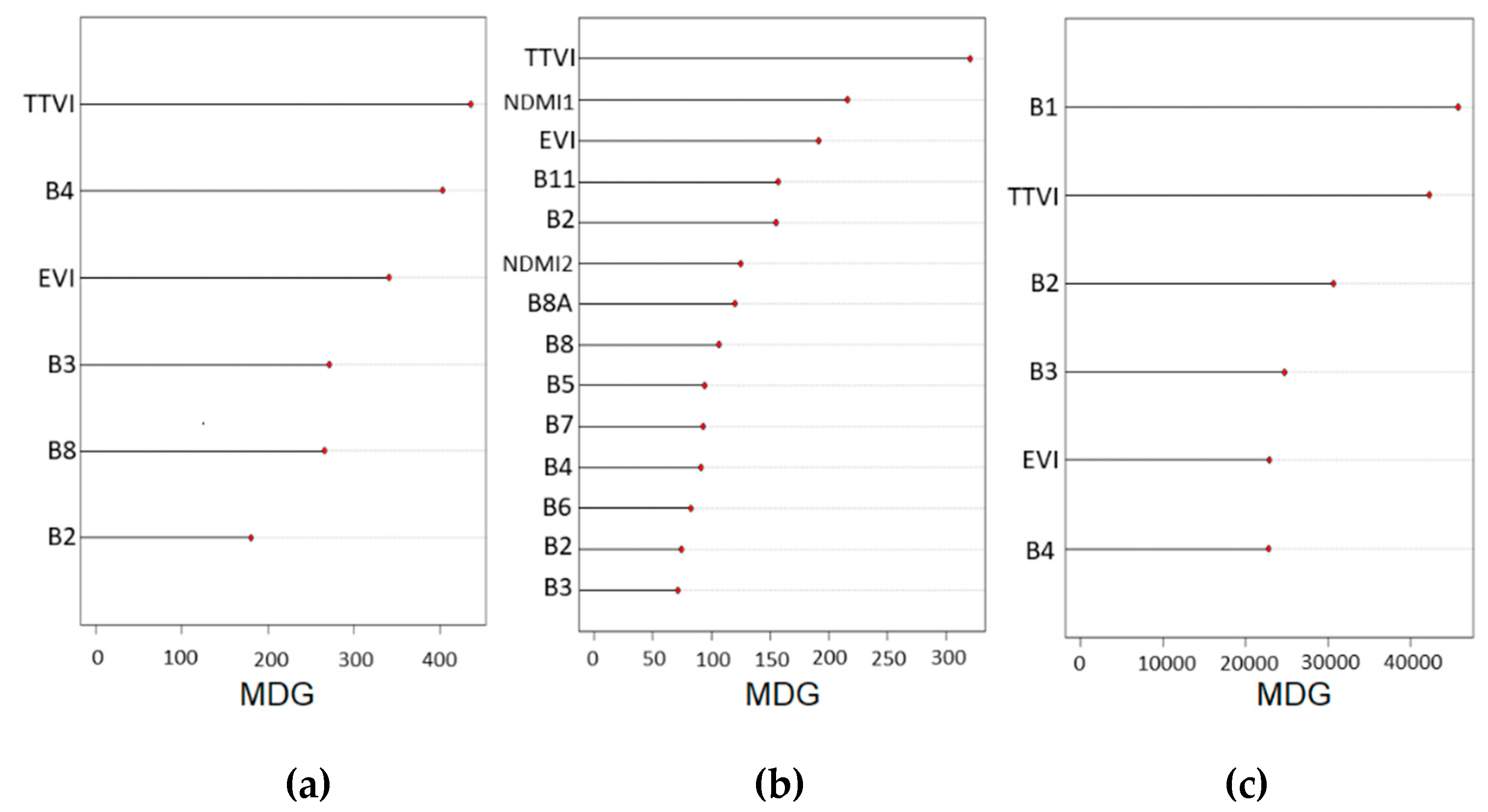
| Model 1 | B2, B3, B4, B8, EVI and TTVI (Sentinel-2) | 6 | 144 | 2847 | 100 | 2 |
| Model 2 | B2, B3, B4, B5, B6, B7, B8, B8A, B11, B12, EVI, TTVI, NDMI1 and NDMI2 (Sentinel-2) | 14 | 144 | 2847 | 100 | 8 |
| Model 3 | B1, B2, B3, B4, EVI and TTVI (High-resolution image) | 6 | 144 | 283,329 | 100 | 2 |
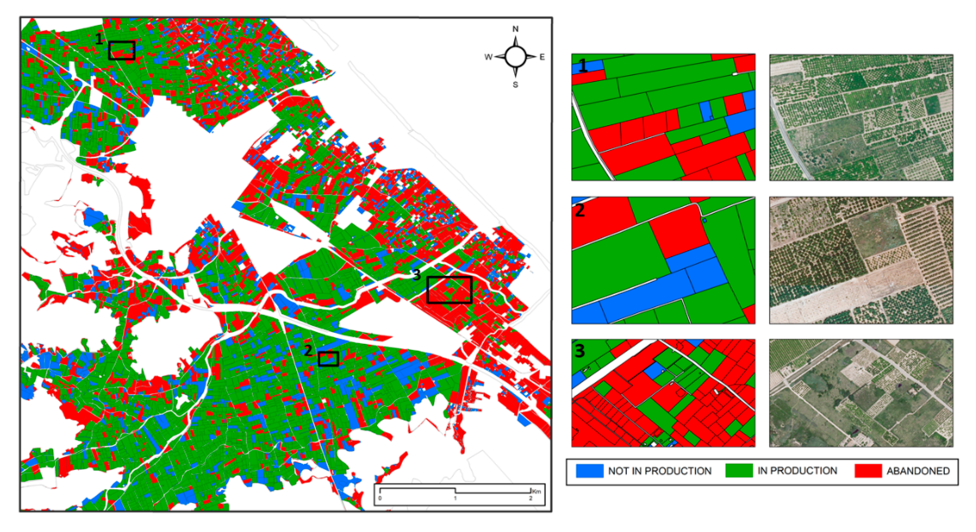
| Not-in-Production Plots | Not-in-Production Surface (%) | In-Production Plots | In-Production Surface (%) | Abandoned Plots | Abandoned Surface (%) | |
|---|---|---|---|---|---|---|
| Model 1 | 2080 | 14.3 | 5069 | 51.0 | 4156 | 34.6 |
| Model 2 | 2308 | 16.0 | 4959 | 51.9 | 4038 | 32.1 |
| Model 3 | 2415 | 15.4 | 4587 | 52.2 | 4303 | 32.2 |
| Overall Accuracy (c.i. 95%) | |
|---|---|
| Model 1 | 77.1% |
| Model 2 | 76.0% |
| Model 3 | 88.5% |
| Model 1 | |||||
| Classified data | Reference Data | ||||
| Not in Production | Inproduction | Abandoned | Total Map | User’s Accuracy | |
| Not in production | 31 | 4 | 2 | 37 | 83.8% |
| In production | 0 | 18 | 5 | 23 | 78.3% |
| Abandoned | 1 | 10 | 25 | 36 | 69.4% |
| Total field | 32 | 32 | 32 | ||
| Producer’s accuracy | 96.9% | 56.3% | 78.1% | ||
| Model 2 | |||||
| Classified Data | Reference Data | ||||
| Not in Production | In Production | Abandoned | Total Map | User’s Accuracy | |
| Not in production | 31 | 3 | 0 | 34 | 91.2% |
| In production | 0 | 17 | 7 | 24 | 70.8% |
| Abandoned | 1 | 12 | 25 | 38 | 65.8% |
| Total field | 32 | 32 | 32 | ||
| Producer’s accuracy | 96.9% | 53.1% | 78.1% | ||
| Model 3 | |||||
| Classified Data | Reference Data | ||||
| Not in Production | In Production | Abandoned | Total Map | User’s Accuracy | |
| Not in production | 32 | 2 | 0 | 34 | 94.1% |
| In production | 0 | 28 | 7 | 35 | 80.0% |
| Abandoned | 0 | 2 | 25 | 27 | 92.6% |
| Total field | 32 | 32 | 32 | ||
| Producer’s accuracy | 100% | 87.5% | 78.1% | ||
© 2020 by the authors. Licensee MDPI, Basel, Switzerland. This article is an open access article distributed under the terms and conditions of the Creative Commons Attribution (CC BY) license (http://creativecommons.org/licenses/by/4.0/).
Share and Cite
Morell-Monzó, S.; Estornell, J.; Sebastiá-Frasquet, M.-T. Comparison of Sentinel-2 and High-Resolution Imagery for Mapping Land Abandonment in Fragmented Areas. Remote Sens. 2020, 12, 2062. https://0-doi-org.brum.beds.ac.uk/10.3390/rs12122062
Morell-Monzó S, Estornell J, Sebastiá-Frasquet M-T. Comparison of Sentinel-2 and High-Resolution Imagery for Mapping Land Abandonment in Fragmented Areas. Remote Sensing. 2020; 12(12):2062. https://0-doi-org.brum.beds.ac.uk/10.3390/rs12122062
Chicago/Turabian StyleMorell-Monzó, Sergio, Javier Estornell, and María-Teresa Sebastiá-Frasquet. 2020. "Comparison of Sentinel-2 and High-Resolution Imagery for Mapping Land Abandonment in Fragmented Areas" Remote Sensing 12, no. 12: 2062. https://0-doi-org.brum.beds.ac.uk/10.3390/rs12122062