Integration of InSAR Time-Series Data and GIS to Assess Land Subsidence along Subway Lines in the Seoul Metropolitan Area, South Korea

Abstract

The aims of this research were to map and analyze the risk of land subsidence in the Seoul Metropolitan Area, South Korea using satellite interferometric synthetic aperture radar (InSAR) time-series data, and three ensemble machine-learning models, Bagging, LogitBoost, and Multiclass Classifier. Of the types of infrastructure present in the Seoul Metropolitan Area, subway lines may be vulnerable to land subsidence. In this study, we analyzed Persistent Scatterer InSAR time-series data using the Stanford Method for Persistent Scatterers (StaMPS) algorithm to generate a deformation time-series map. Subsidence occurred at four locations, with a deformation rate that ranged from 6–12 mm/year. Subsidence inventory maps were prepared using deformation time-series data from Sentinel-1. Additionally, 10 potential subsidence-related factors were selected and subjected to Geographic Information System analysis. The relationship between each factor and subsidence occurrence was analyzed by using the frequency ratio. Land subsidence susceptibility maps were generated using Bagging, Multiclass Classifier, and LogitBoost models, and map validation was carried out using the area under the curve (AUC) method. Of the three models, Bagging produced the largest AUC (0.883), with LogitBoost and Multiclass Classifier producing AUCs of 0.871 and 0.856, respectively.

1. Introduction

Land subsidence is a threat faced by big cities with extensive development that can negatively impact the environment, social systems, and the economy [1]. Subsidence occurs due to geological causes or anthropogenic processes such as massive urban development, infrastructure development [2,3], tunneling [4,5,6], water extraction [7,8,9], and earthquakes [10]. Subsidence has been observed in several metropolitan cities, including Mexico City [11], Shanghai [12], and Jakarta [13,14,15]. The Seoul Metropolitan Area is the center of governance, commerce, and culture in South Korea. It has been extensively developed and is the most densely populated city in Asia [16]. Industrial development and economic growth have led to city developments such as the expansion of subway lines and the construction of many structures and buildings [17]. By examining the potential effects of land subsidence, monitoring of land deformation could be the first step of a mitigation process. Seoul, which has a high population density and extensive developments, is extremely vulnerable to land subsidence. Given the severe negative impacts of subsidence, it necessary to elucidate the factors that cause land subsidence from integrated observations, to assess damage risks and prevent damage to roads, bridge, railways, and other infrastructure.

Monitoring land deformation is essential for reducing losses due to subsidence and developing a sound mitigation plan. With advancements in knowledge and technology, monitoring techniques have improved greatly. Previously, measurements related to land subsidence could be taken using traditional geodetic [15] and leveling methods, which provide precise measurements, but these methods are inefficient and costly compared with satellite-based methods, which cover broader areas and are more cost-efficient. These days, more studies are using satellite-based synthetic aperture radar (SAR) to monitor land deformation. SAR is an advanced remote-sensing technology that has been used worldwide in several applications; it is considered active remote sensing as the sensor emits its own microwaves before recording the backscattered waves [18]. In addition, another advantage of SAR is its flexibility in acquiring data, as it can operate under any weather conditions and all day [19]. Thus, because of its operational flexibility, SAR is considered reliable for damage assessment and risk analysis.

Recently, there has been growing interest in monitoring ground deformation using differential interferometric SAR (DInSAR), which is used to estimate such small deformation. However, this method is often restrained by temporal decorrelation and atmospheric disturbance. Those problems are difficult to eliminate when estimating the representative interferograms of ground deformations [20]. To solve this problem, a long-term InSAR processing approach using a series of data, generally recognized as time-series InSAR analysis. Time-series analysis has been widely used for ground-monitoring projects, such as monitoring urban areas, groundwater, and land subsidence [21,22,23]. An example of InSAR time-series methods that have been developed in recent years is Persistent Scatterer InSAR (PS-InSAR). With time-series data accumulated over long periods of monitoring, deformation can be measured over broader areas, and the occurrence of deformation in an area can be studied with more precision compared to data from conventional InSAR methods. In addition, a prominent advantage of time-series analysis is a reduction in issues related to InSAR, such as temporal decorrelation and atmospheric interference.

In PS-InSAR, multiple large SAR images of the same area are processed, which can extract a number of persistent scatterers (PS) [24]. This method focuses on measuring the level of deformation associated with each of the persistent scatterers, which is a point of high density within an interferogram from a single main image. Therefore, this technique was developed for urban areas, which have more stable scatterers than mountains or forests with distributed scatterers [25]. In recent years, many PSI approaches have been developed and applied in many cases, such as PS-InSAR [26,27,28], Stable Point Network (SPN) [29], Interferometric Point Target Analysis (IPTA) [30,31,32], and Stanford Method of Persistent Scatterers (StaMPS) [33,34]. This method has been applied to measure deformation in several locations such as West Macedonia, Greece [35]; Nile Delta, Egypt [23]; Tuscany and Northern Apennines, Italy [20,36,37]; Mexico City, Mexico [11]; and Guangzhou, China [30,38].

In general, susceptibility maps are generated as part of land-subsidence mapping and modeling. These maps are used to predict and examine areas that are highly vulnerable to land subsidence and are important as part of the initial information used to prevent future land-subsidence events, assuming the same conditions will trigger land subsidence in the future [39]. Land-subsidence analysis largely focuses on elucidating the sources of subsidence, methods of evaluation, understanding subsidence events on a conceptual level, and mapping [40]. Remote sensing and Geographical Information System (GIS) analysis are commonly employed in hazard studies because of the efficiency of these techniques in data collection and analysis [41]. The utility of several GIS methods in terms of generating subsidence-susceptibility maps has been compared using statistical tools such as frequency ratio and weight of evidence [6,37]. Artificial neural networks, random forests, and fuzzy logic have also been applied to assess methods of predicting subsidence susceptibility [42,43,44]. Furthermore, machine-learning techniques have recently attracted attention in the environmental-modeling research community as they are highly efficient and generate improved outcomes.

Previous studies related to land subsidence in Seoul related to the risk analysis of ground subsidence around railways using ANN modeling [45]. However, studies related to land subsidence in Seoul are needed to map the potential for land subsidence and understand the causes that can lead to land subsidence. In this study, we aimed to examine ground deformation within the 2017–2020 time period in the Seoul Metropolitan Area using C-band data from the Sentinel-1 satellite. The velocity of land subsidence and the associated land deformation was investigated via Stanford Method for Persistent Scatterers (StaMPS), and a deformation time-series map was generated. The map was used as input data for a land-subsidence inventory map, which was then used to generate a land-subsidence-susceptibility map. GIS analysis was employed to complement observations of land subsidence in the urban area. Thereafter, the performance of the meta-ensemble methods in terms of land-subsidence-susceptibility modeling was assessed. The LogitBoost, Multiclass Classifier, and Bagging functional models were used as they have been shown to improve the performance of predictive models in several cases of susceptibility map [43,46,47]. Bagging more effectively reduces the bias compared to other ensembles, while LogitBoost is used to solve the overfitting problem [43,48]. Model performance in terms of predicting land-subsidence susceptibility was assessed using training and testing datasets, receiver operating characteristic (ROC), and the area under the curve (AUC). The area under the curve of the roc represents the validation of systems and its ability to predict the correct occurrence or non-occurrence of land subsidence events [49]. The ROC graph is a technique for visualizing, organizing, and selecting classifier based on their performance. Then, the area under the curve is a common method to calculate the area under the curve to compare the classifiers and convert it to the scalar values which represent the performance [50]. By linking time-series data with GIS analysis, the research findings will increase our understanding of crucial factors affecting ground surface areas. The map of ground-deformation risk in an urban area generated in this study reflects the association between subsidence risk and risk factors; this information would help identify areas of high risk and develop environmental action plans and policies.

2. Materials & Methods

2.1. Study Area

Seoul is the capital city of South Korea. It is located in the midwestern region of the Korean Peninsula at 126°59′40″E and 37°33′59″N and covers an area of 605.5 km² [51]. The Han River, which is one of the largest rivers crossing Seoul, divides the city into north and south areas. Seoul has a population of approximately 10 million people with a density of 16,364 people/km², making it one of the most populous metropolitan cities in Asia [52]. The geological setting of Seoul consists of Jurassic granite, Precambrian metamorphic rocks (gneiss and schist), and Quaternary alluvium. Predominantly, coarse-grained, sandy alluvium sequence (<20 m thick) occurs along the Han River and its tributaries [53]. The alluvium is mainly distributed along the Han River and its tributaries, it is composed of coarse- to fine-grained sediments, often with high permeability. The alluvium and soil tend to be thicker close to the river, particularly its lower reaches, and thinner in mountain area [54]. In this study area, there are two types of aquifer unconsolidated alluvium aquifers and bedrock aquifers [17]. The alluvial aquifers are dominantly composed of silt and fine to coarse sands are appearance along the Han river and tributaries. The bedrock aquifers are mainly composed of fractured gneiss, schist, and granite.

As a metropolitan city that has experienced urbanization in recent years, Seoul has experienced many developments such as office, business, and residential buildings. This has an impact on increasing the density of the building in this area. The use of groundwater and other utilities in densely populated areas will have an impact on the weakening of soil conditions in these areas. This condition can indirectly lead to subsidence which can cause many losses, especially in areas with high population density such as Seoul.

Together with the increase in population, the economy has grown quickly, followed by industrial development. To meet the needs of the city inhabitants, Seoul undertook massive developments, including infrastructure, buildings, and transportation networks. At the end of 2019, a total of 23 rapid transit, light metro, commuter rail, and airport rail lines had been integrated into the Seoul Metropolitan Subway system [55]. This system operates in the Seoul Metropolitan Area, including Incheon and some satellite cities in Gyeonggi Province. Several regional lines such as those in Chungnam and Gangwon provinces are also connected to this system. Figure 1 has shown a map of the subway line that has been operating and in the process of construction in the Seoul Metropolitan Area. New transportation routes have since been added, such as the Gimpo Gold-Line in 2019, and the Line 7 and Line 5 extensions to Hanam City is currently under construction and slated to open in 2020. To improve connectivity in this metropolitan area, several future subway lines (until 2028) are still being planned.

In densely populated areas like Seoul, ground subsidence can cause much higher casualties and property damages than in lesser populated areas. For this reason, it is of utmost importance to conduct complete monitoring on the cases of ground subsidence to prevent damages on roads, railroads, and other infrastructures.

2.2. SAR Datasets

In this study, SAR data from Sentinel-1B was used to generate representations of surface deformation. SAR images derived from C-band data can be used to map surface deformation over broad areas while providing time-consistent ground-deformation data. Sentinel-1B has an acquisition cycle of 12 days. We used 93 SAR scenes from descending tracks. The descending datasets are listed in

Table 1. Acquisition dates of data from the Sentinel-1 satellite in descending tracks, the reference date shown in bold text.

No.	Acquisition Date (yyyymmdd)	Days	$\mathbf{B}\perp \left(\mathbf{m}\right){}^1$	No.	Acquisition Date (yyyymmdd)	Days	$\mathbf{B}\perp {\left(\mathbf{m}\right)}^1$	No.	Acquisition Date (yyyymmdd)	Days	$\mathbf{B}\perp \left(\mathbf{m}\right){}^1$
1	20170302	−588	78	32	20180414	−180	102	63	20190421	192	125
2	20170314	−576	128	33	20180426	−168	67	64	20190503	204	187
3	20170326	−564	128	34	20180508	−156	39	65	20190515	216	97
4	20170407	−552	91	35	20180520	−144	17	66	20190527	228	91
5	20170419	−540	61	36	20180601	−132	−2	67	20190620	252	82
6	20170501	−528	83	37	20180613	−120	117	68	20190702	264	160
7	20170513	−516	117	38	20180625	−108	87	69	20190714	276	117
8	20170525	−504	82	39	20180707	−96	65	70	20190807	300	41
9	20170606	−492	121	40	20180719	−84	93	71	20190819	312	100
10	20170618	−480	49	41	20180731	−72	24	72	20190831	324	87
11	20170630	−468	14	42	20180812	−60	67	73	20190912	336	99
12	20170712	−456	91	43	20180824	−48	69	74	20190924	348	112
13	20170805	−444	129	44	20180905	−36	77	75	20191006	360	55
14	20170817	−420	12	45	20180917	−24	62	76	20191018	372	103
15	20170910	−408	78	46	20180929	−12	74	77	20191030	384	64
16	20170922	−384	134	47	20181011	0	0	78	20191111	396	132
17	20171004	−372	105	48	20181023	12	163	79	20191123	408	126
18	20171016	−360	96	49	20181104	24	109	80	20191205	420	66
19	20171028	−348	96	50	20181116	36	106	81	20191217	432	110
20	20171109	−336	71	51	20181128	48	70	82	20191229	444	163
21	20171121	−324	126	52	20181210	60	122	83	20200110	456	176
22	20171203	−312	150	53	20181222	72	190	84	20200203	480	101
23	20171215	−300	148	54	20190103	84	119	85	20200215	492	61
24	20171227	−288	103	55	20190115	96	58	86	20200227	504	70
25	20180108	−276	102	56	20190127	108	96	87	20200310	516	158
26	20180201	−264	159	57	20190208	120	141	88	20200322	528	141
27	20180213	−240	166	58	20190220	132	174	89	20200403	540	80
28	20180225	−228	44	59	20190304	144	157	90	20200415	552	46
29	20180309	−216	−7	60	20190316	156	31	91	20200427	564	63
30	20180321	−204	−35	61	20190328	168	29	92	20200509	576	72
31	20180402	−192	126	62	20190409	180	68	93	20200521	588	56

¹ B$\perp$: Perpendicular Baseline.

, the reference date with zero delta day and zero perpendicular baselines from the descending track is shown on October 11, 2018 as the reference date are shown in bold text.

2.3. StaMPS Processing

One of the known methods for generating time-series data on surface deformation is StaMPS, as it can be used for analysis on the urban area like this study area. This method is commonly recognized on man-made objects such as buildings, infrastructure, and roads in urbanized areas like Seoul. Another major advantage of this method is that it does not require a prior deformation model, thus allowing analysis of different regions and several deformation causes [24].

At the start of PSI-StaMPS analysis, the interferogram process was begun to generate a couple of interferogram images from the 93 SAR scenes in descending track. Prior to interferogram generation, SAR data underwent a co-registration process, in which two SAR images were aligned to subpixel accuracy for accurate determination and noise reduction to form interferometric pairs. The SAR images were then resampled such that the slave images matched the master image. When the co-registration process was complete, the co-registered images were cropped to focus on the study area before the interferogram generation process began. During the interferogram processing stage, a topographical phase was generated. Once the interferogram images were generated, the topographic phase was subtracted from the interferogram using Shuttle Radar Topography Mission digital elevation model (SRTM DEM) as the reference [56]. After the topographic phase was removed, a DInSAR phase was generated, which contained only the deformation phase.

For StaMPS processing, SAR data on 11 October 2018 was chosen as a master image and generated 92 interferograms from the descending track. After generating the interferograms, the StaMPS module was used to calculate the displacements of persistent scatterers. To begin the StaMPS process, phase stability estimation was used to select a subset of pixels based on amplitude analysis. Then, phase stability for each pixel was estimated through phase analysis [57]. Once the phase noise associated with all selected persistent scatterer (PS) pixels was estimated, the selected PS pixels were weeded out to separate the persistent points and noise, then the wrapped phase of the selected pixels was corrected for spatially-uncorrelated look-angle errors in the DEM. After correction, the corrected phase could now be unwrapped, and the PS output was generated. The parameter of the StaMPS process is shown in

Table 2. The parameter in StaMPS processing.

Parameter	Value
DEM	SRTM 1 arc second
Maximum DEM error	20 m
Band-pass phase filter grid size	50
Band-pass phase filter low-pass cutoff	800
Band-pass phase filter low-pass α	1
Band-pass phase filter low-pass β	0.3
Unwrapping algorithm	3D unwrapping
Unwrapping grid cell size	100
Unwrapping Gaussian width	8σ

. Upon completion of the StaMPS process, PS results were plotted in a time-series map and a mean deformation from the line of sight (LOS) map [58,59]. The mean deformation map is converted into vertical deformation data by assuming the horizontal deformation is very small compared to the vertical deformation that causes by land subsidence [60,61]. In recent studies, the vertical deformation was used to monitor land subsidence in several places, therefore horizontal deformation in this study can be assumed as negligible and converted into vertical deformation value [13,14]. The result of vertical deformation will be assigned as a negative value from initial ground-level observation, which indicates the land subsidence measure vertically on that point. The vertical deformation can be calculated using this Equation (1) as follows [62]:

$$\mathrm{V}=\frac{{\mathrm{d}}_{\mathrm{LOS}}}{\cos \mathsf{\theta }}$$

(1)

where ${\mathrm{d}}_{\mathrm{LOS}}$ is the deformation in line of sight and $\mathsf{\theta }$ is the incident angle.

2.4. Generation of Susceptibility Map

The workflow to generate land subsidence susceptibility maps, using machine learning algorithms, is illustrated in Figure 2, the summary of the methodology is as follows:

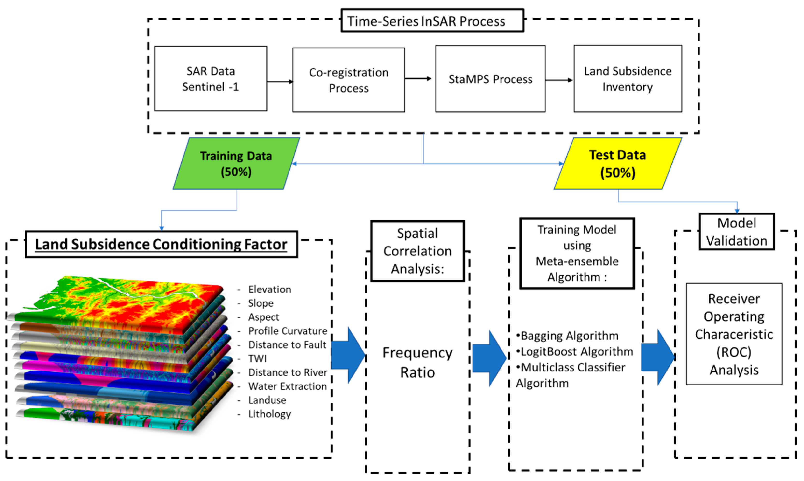
• The land subsidence inventory was generated by analyzing Sentinel-1 SAR datasets from 2017 to 2020 from descending tracks using the time-series InSAR technique based on StaMPS algorithms.
• In order to generate land susceptibility maps, the training and test datasets were prepared by randomly divided the persistent scatterers (PS) points of time series into 50% of training data and 50% of testing datasets to validate the land subsidence susceptibility map. Training data is used to train the machine learning to predict subsidence in our land subsidence susceptibility model. Besides, test data is used to measure the performance, of the algorithm that we used to make the land subsidence susceptibility model. This preparation method of training and testing datasets was used in several studies of land subsidence susceptibility which has optimal results [6,63,64].
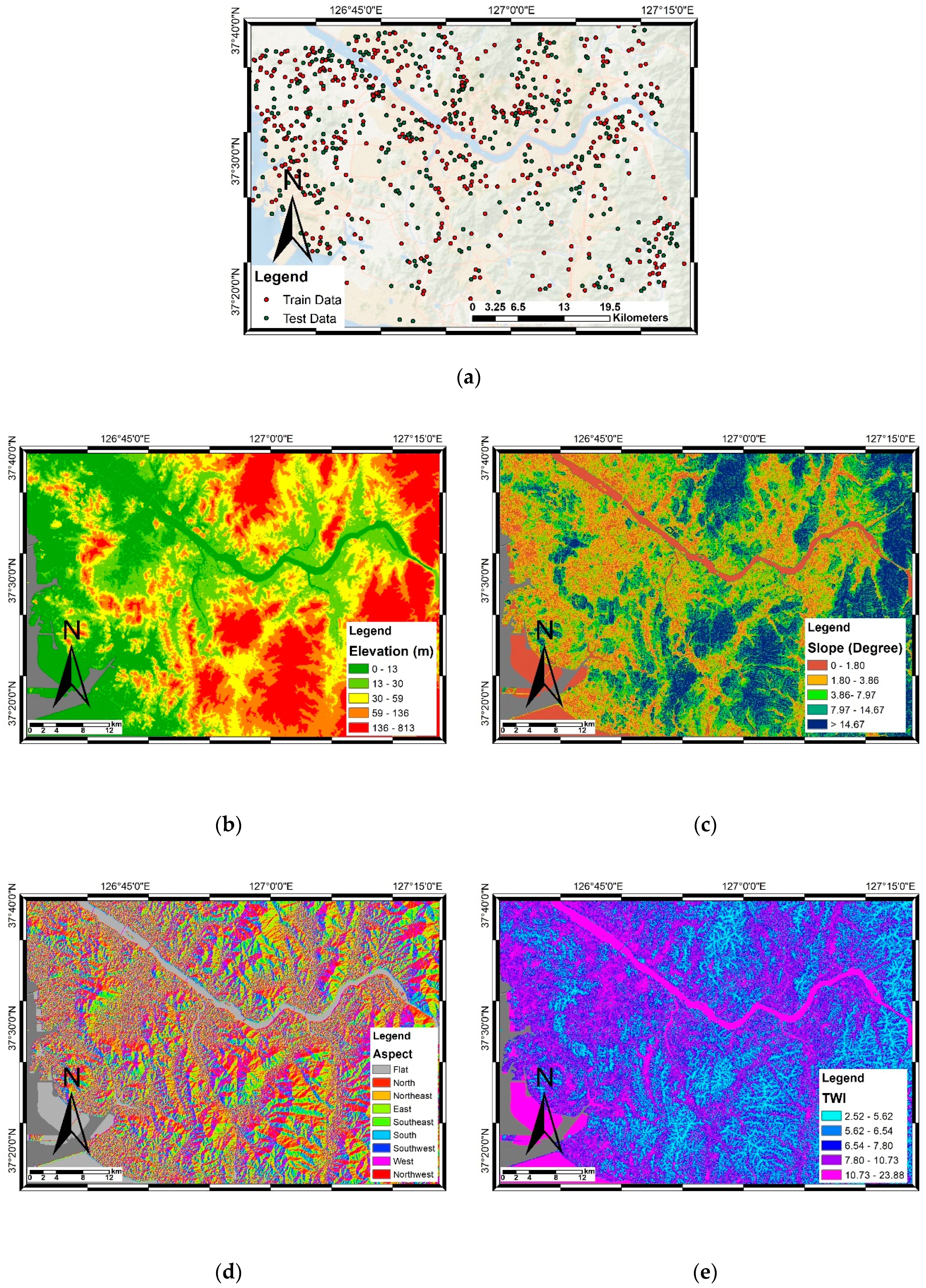
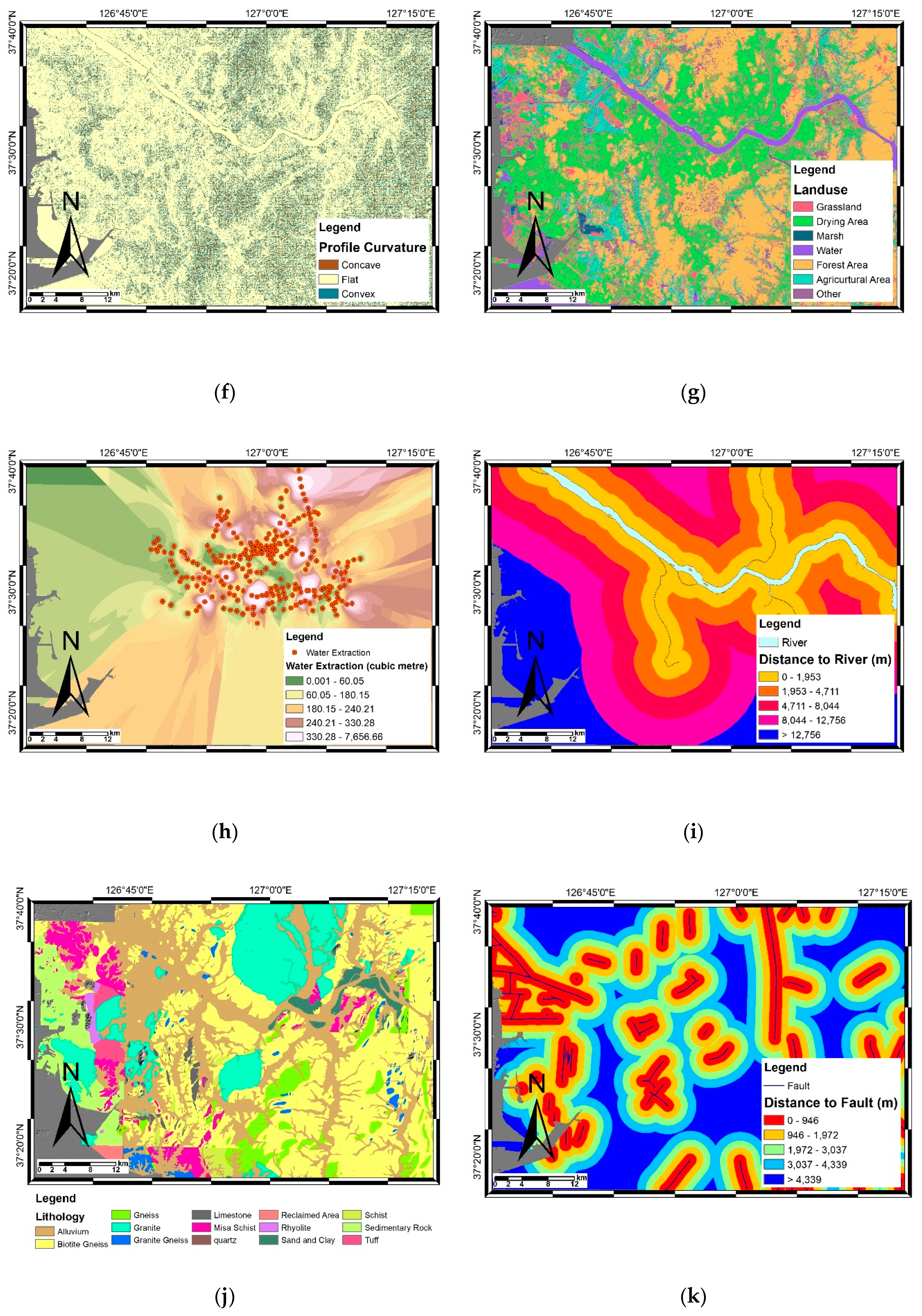
• Preparation of land subsidence conditioning factors: Spatial correlation analysis was applied to assess each factor before the land-subsidence model was generated. In the spatial correlation analysis, the spatial relationship between historical subsidence events, and each factor was examined [65]. Spatial correlation analysis was also used to investigate the weight of each factor class to assess the strength of the relationship between each factor class and subsidence occurrence. Frequency ratios were calculated to reflect spatial correlations by calculating the proportion of cells in which subsidence occurred in each class; then, factors were reclassified. Frequency ratios have been commonly used to determine spatial correlations [40,42,66]. Here, each frequency ratio represents the quantitative relationship between subsidence in a selected class and all subsidence in the area for all classes as a percentage of the entire map [67]. If the ratio is greater than one, the relationship between subsidence and the factor class is considered strong. By contrast, if the ratio is less than one, the spatial relationship is weak [40].
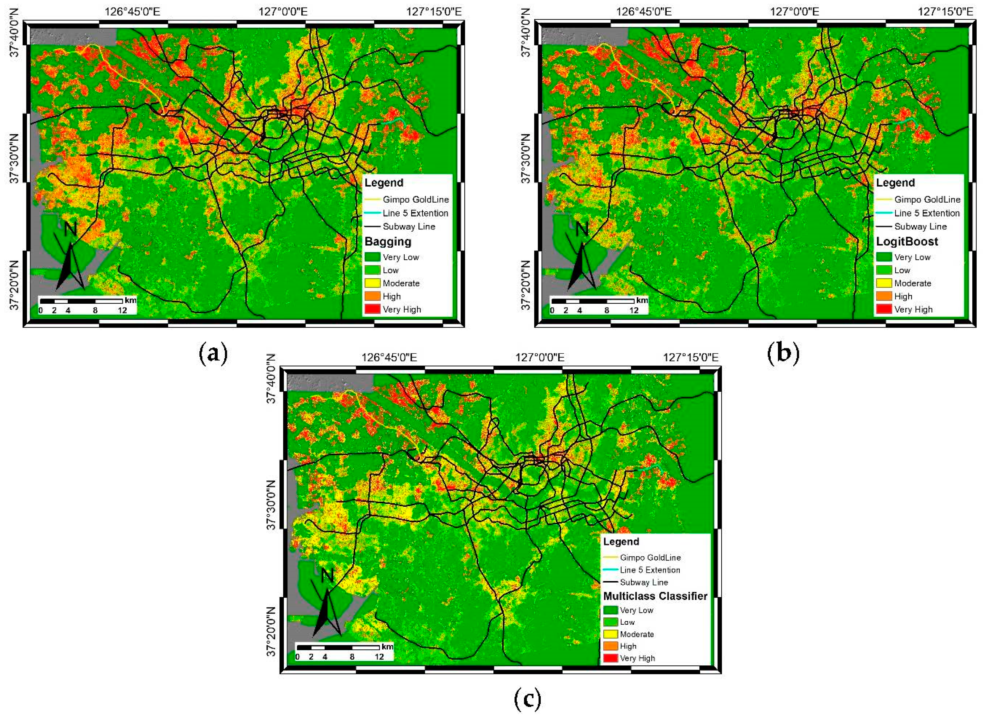
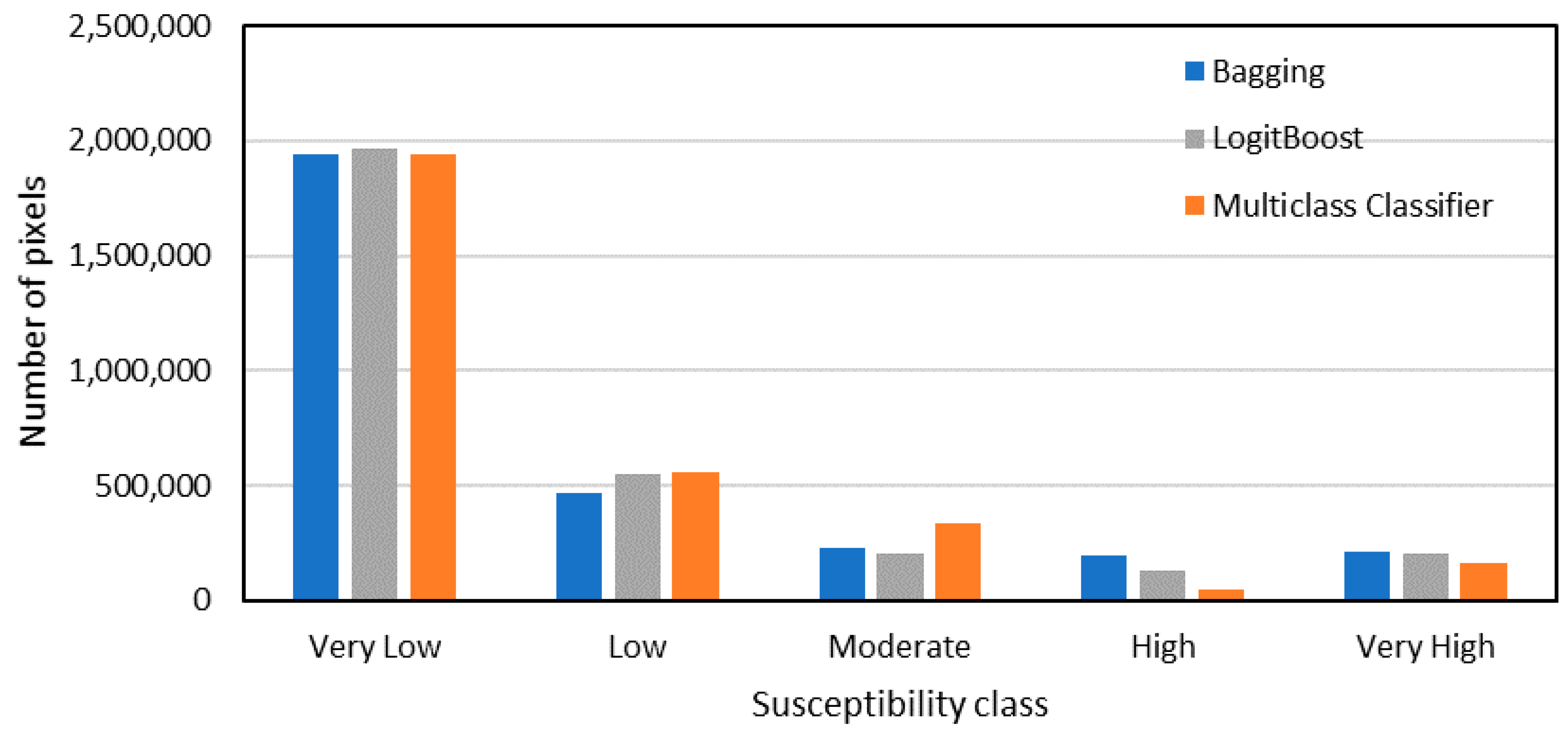
• Generating land subsidence susceptibility map: in this step, we constructed a land subsidence susceptibility map using Bagging, LogitBoost, and Multiclass Classifier algorithms. The land subsidence conditioning factors that consist of frequency ratio values.
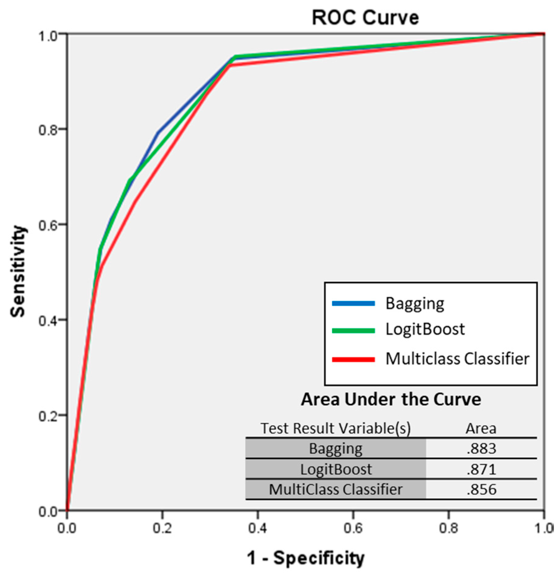
• After the land subsidence susceptibility map was generated, all susceptibility maps were evaluated using ROC analysis.

2.4.1. Bagging

Bagging is a commonly used meta-algorithm that was developed to enhance the stability and accuracy of the machine-learning algorithms used in statistical classification and regression [43]. Bagging was one of the earliest ensemble techniques that used the bootstrap sampling method [68]. The bootstrap method entails apparent random sampling with replacements to generate more than one sample that shapes a training set. Each generated subset is used to assemble a decision tree, with all trees aggregated later into the final model. This improves class accuracy by reducing the variance of class error. We used Bagging to obtain a much improved and more accurate land subsidence model because this algorithm performs well in predicting land subsidence susceptibility, as it is sensitive to small adjustments in the training data and consequently [43,46]. Bagging ensembles more effectively reduce uncertainty and bias compared to other ensembles [69]. In addition, this algorithm is capable of reflecting complex non-linear interaction between land subsidence and related factors, although it lacks a statistical significance test which can limit quantitative hypothesis testing [43]. Bagging first uses a classifier to reduce variance, then carries out classification and regression by relying on bottom-up learning.

2.4.2. LogitBoost

LogitBoost is a boosting algorithm developed by Friedman et al., [70] to reduce bias and variance. The LogitBoost algorithm was modified from AdaBoost, which was the commonly boosting method for handling noisy data that execute additive logistic regression with least-square fits for individual class [48,71]. LogitBoost reduces training errors and enhances classification accuracy [72] by using additive logistic regression for classification with a base-learning regression scheme and an ability to perform multiclass classification. The land subsidence-inventory map was divided into two classes—subsidence occurrence and subsidence non-occurrence—using the following equation [71]:

$$\mathrm{Lc}\left(\mathrm{c}\right)={\displaystyle \sum }_{i=1}^{\mathrm{D}}{\mathsf{\beta }}_i{\mathrm{x}}_i{+\mathsf{\beta }}_0$$

(2)

where D is the number of landslide-dependent factors and ${\mathsf{\beta }}_i$ is the coefficient of the i-th component within input vector $\mathrm{x}$. Probabilities were constructed using the linear logistic regression method, as follows:

$$\mathrm{p}\left(\frac{\mathrm{C}}{\mathrm{x}}\right)=\exp \left(\mathrm{Lc}\left(\mathrm{x}\right)\right)/{\displaystyle \sum }_{{\mathrm{C}}^{\prime }=1}^{\mathrm{C}}{\exp (\mathrm{Lc}}^{\prime }(\mathrm{x}))$$

(3)

where C is the number of classes and the least-square fit $\mathrm{Lc}\left(\mathrm{x}\right)$ is resolved such ${\displaystyle \sum }_{\mathrm{C}=1}{\mathrm{L}}_{\mathrm{C}}^{\mathrm{C}}\left(\mathrm{x}\right)=0$ to set up the least number of instances per node of the logistic model trees.

2.4.3. Multiclass Classifier

Multiclass Classifier is a meta-classifier that is used to process multiclass datasets with two-class classifiers. It is efficient at applying error-correcting output codes to enhance accuracy [47]. In the field of machine learning, multiclass classification can classify events into one of three or more classes. Although several classification algorithms can work with more than two classes with the aid of natural binary algorithms, the conversion to multinomial classifiers requires the use of several strategies. Multiclass classification techniques can be divided into categories such as transformation to binary, extension from binary, and hierarchical classification [73].

2.5. Factors Related to Land Subsidence

The increase in land subsidence occurrence in megacities mainly due to lowered groundwater levels and the presence of heavy buildings [17]. Excessive use of groundwater has an impact on decreasing pore pressure on the soil, coupled with the presence of heavy buildings that lead to further soil compaction [74,75]. A large amount of groundwater leaked, and dewatering accompanies a decrease in groundwater levels. Those conditions weaken the surrounding land and lead to subsidence occurrence. In addition, based on a report by the Seoul government which has conducted field investigations, one of the causes of subsidence is excessive groundwater use and damage to water utilities and sewage [3,17].

A combination of several environmental factors can influence land-subsidence susceptibility. The training data and test data point was chosen from the land subsidence inventory map as shown in Figure 3a. Here, we investigated 10 subsidence-related factors (Figure 3b–k) and evaluated the correlation between each factor and land-subsidence occurrence as shown in

Table 3. Frequency Ratio calculation.

Conditioning Factor	Class/Category	Ratio each Class	Ratio of Occurrence	FR
Elevation	0–13	0.205	0.292	1.424
	13–30	0.206	0.355	1.722
	30–59	0.198	0.228	1.147
	59–136	0.197	0.100	0.510
	136–813	0.194	0.025	0.130
Aspect	Flat	0.066	0.071	1.071
	North	0.113	0.117	1.029
	Northeast	0.127	0.122	0.958
	East	0.125	0.132	1.059
	Southeast	0.128	0.135	1.053
	South	0.125	0.122	0.972
	Southwest	0.135	0.125	0.925
	West	0.124	0.121	0.976
	Northwest	0.056	0.056	0.999
Profile	concave	0.085	0.041	0.480
	flat	0.821	0.900	1.096
	convex	0.094	0.059	0.629
Slope	0–1.8	0.132	0.193	1.460
	1.8–3.86	0.218	0.350	1.601
	3.86–7.97	0.216	0.275	1.273
	7.97–14.67	0.216	0.142	0.656
	> 14.67	0.217	0.040	0.185
Topographic Wetness Index	2.52–5.62	0.207	0.072	0.347
	5.62–6.54	0.224	0.184	0.823
	6.54–7.80	0.228	0.264	1.157
	7.80–10.73	0.216	0.321	1.484
	10.73–23.88	0.125	0.159	1.270
Land use	Drying Area	0.318	0.658	2.069
	Agriculture Area	0.078	0.073	0.929
	Forest Area	0.316	0.049	0.157
	Grassland	0.125	0.148	1.183
	Marsh	0.023	0.007	0.308
	Other	0.058	0.053	0.900
	Water Body	0.081	0.012	0.145
Distance to River (m)	0–1953	0.214	0.294	1.372
	1953–4711	0.218	0.261	1.195
	4711–8044	0.218	0.172	0.786
	8044–12,576	0.215	0.166	0.773
	> 12,576	0.135	0.108	0.801
Groundwater Extraction (m3/day)	0–60	0.108	0.161	1.497
	60–180.15	0.314	0.339	1.081
	180.15–240.21	0.027	0.021	0.782
	241.21–330.28	0.272	0.192	0.706
	> 330.28	0.280	0.287	1.024
Distance to Fault (m)	0–946	0.212	0.252	1.188
	946–1972	0.207	0.213	1.031
	1972–3307	0.203	0.188	0.929
	3307–4339	0.199	0.191	0.960
	> 4339	0.180	0.156	0.868
Lithology	Qa	0.304	0.422	1.385
	PCEbgn	0.054	0.024	0.442
	PCEbngn	0.307	0.223	0.725
	PCEggn	0.011	0.007	0.609
	PCElbgn	0.003	0.000	0.000
	pgr	0.005	0.004	0.809
	Jsgr	0.045	0.068	1.518
	Jbgr	0.054	0.061	1.136
	PCEms	0.043	0.049	1.151
	PCEls	0.006	0.001	0.166
	Kkt	0.003	0.002	0.749
	rc	0.054	0.088	1.615
	PCEagn	0.010	0.002	0.199
	qz	0.001	0.000	0.228
	Qd	0.014	0.019	1.390
	Krh	0.004	0.004	0.992
	Qc	0.001	0.002	1.327
	mgn	0.003	0.000	0.000
	PCEpgn	0.009	0.002	0.215
	Jdgr	0.021	0.006	0.275
	PCEfgn	0.009	0.002	0.243
	PCEbs	0.005	0.002	0.423
	PCElgn	0.007	0.002	0.267
	Kct	0.006	0.004	0.686
	PCEqfgn	0.003	0.000	0.171
	PCEqf	0.003	0.000	0.000
	PCEsch	0.006	0.002	0.319
	PCEqgn	0.004	0.000	0.000
	Qr	0.004	0.004	0.873

below. In the previous studies, land subsidence conditioning factors such as altitude, slope, aspect, plan curvature, profile curvature, lithology, distance to the river, land use, normalized differential vegetation index (NDVI), piezometric data (groundwater drawdown) have been used with the main cause of subsidence in Iran being groundwater drawdown [49]. Another study has evaluated several factors mentioned before to identify land subsidence in the mining area in Malaysia [40]. Reclassification was employed to place subsidence related-factors into several classes using the quantile method to objectively identify and analyze the effect of each class using a specific range of values. The quantile classification method can solve unbalanced distribution by focusing on the equality of domain grids [76]. Thus, the range of each class is automatically determined based on the quantile method.

The derivative feature from the digital elevation model (DEM) contains hydrogeological and topographic conditions such as hydrological zone response, concentration, and containment of runoff volume in the landscape, which directly or indirectly affect the occurrence of land subsidence. The topography features such as elevation, slope, aspect, topographic wetness index (TWI), and profile curvature (Figure 3b–f) data were extracted using SRTM DEM 1 arc second. This feature has been widely used as conditional factors in the land subsidence susceptibility model [37,43,49]. Elevation has a role as a bridge between lithology and rain characteristics in the area. A higher area has a lower probability of additional precipitation than a lower area which has the potential to have high precipitation [49]. The elevation refers to the height of the study area which varies between 0–813 m.

Slope and aspect factor as a secondary feature of DEM may relate to the land subsidence occurrence because it can affect the soil infiltration in the landscape and water utility conditions [77,78]. The groundwater or sewage infiltration through a damaged pipe may erode the soil particles [77]. That condition can indirectly affect soil conditions that lead to land subsidence occurrence.

TWI is a secondary topographic variable that specifies the degree of water accumulation in a certain location; it is commonly used to quantify topographic influence on hydrological processes. The TWI of this study area was prepared based on the DEM and categorized into five classes. Profile curvature is a geomorphic property which shows the flow intensity, the amount of sediment, and erosion [79]. The profile curvature map was categorized into three classes: convex (less than −0.01), flat (−0.01–0.01), and concave (larger than 0.01).

Land-use is related to the ecological conditions and anthropological activities of land subsidence occurrence [80,81]. Variation in land use can explain the highly dissected zones within the region and provide insight into the land subsidence activity that is likely to occur. A land-use map was created based on a digital characteristics map provided by (National Geographic Information Institute) NGII; six land-use categories were analyzed in this study and the map is shown in Figure 3g. Underground water utilities are one of the most frequently cited factors impacting land subsidence [54,82].

Groundwater extraction can correlate to land subsidence event, especially in the underground structure [49]. Groundwater extraction map of this study area was prepared from annual average groundwater outflow data measured in 231 points from Seoul Government. Prior to spatial analysis, data on groundwater extraction should be converted into raster data. The accuracy of the raster map depends on the number of data points; however, the availability of groundwater data was limited in this study. To generate raster maps from these limited data, we applied the inverse distance weighted method to make statistical inferences using observed values before interpolating to create raster maps of groundwater extraction with a 30 m × 30 m cell size as shown in Figure 3h.

In order to evaluate the relationship between groundwater conditions and the occurrence of subsidence, several factors related to groundwater conditions can be evaluated such as distance to rivers [43,83]. The distance to rivers is represented by the proximity of the rivers and drainages in the study area [40]. The distance to the river map was calculated based on the map of the river provided by the National Geographic Information Institute (NGII). Then, buffers around the river were created (measured in meters), then the raster map was divided into five classes as shown in Figure 3i.

The geological parameters of a certain area may influence the occurrence of land subsidence, which is related to the lithological and structural variation which leads to differences in strength and permeability of rocks and soil. Lithology has also been an important feature to understand the land subsidence process by describing the structure of underground materials, as most cases of subsidence occurred on landfills and alluvium layers that have natural consolidation. Besides, the groundwater withdrawal and load from the building induce the compaction rate of the alluvium [17,62]. Any fluid present in the porous medium structure is under pressure because of the weight of the structure above it. If the fluid is withdrawn from below the surface, a decrease in pore pressure can occur, resulting in the loss of the supports and possibly lead to subsidence [74]. The lithology map can be seen in Figure 3j and the description of the lithology is shown in

Table 4. Description of the lithological units in the study area.

Lithology ID	Description	Group
PCEagn	Granular gneiss	Gneiss
PCEfgn	Fine granitic gneiss
mgn	Hybrid gneiss
PCElgn	White matter gneiss
PCElbgn	Lower arcuate gneiss
PCEqfgn	Quartz feldspar gneiss
PCEqf	Filigree gneiss
PCEqgn	Quartz feldspar
Jbgr	Biotite granite	Granite
pgr	Geojeong Pyeonsang Granite
Jsgr	Selenite granite
PCEbgn	Arctic black mica gneiss	Biotite Gneiss
PCEbngn	Biotite Granite
PCEggn	Granitic gneiss	Granite Gneiss
Krh	Rhyolite	Rhyolite
Kkt	Lapiri tuff (mostly fused tuff)	Tuff
PCEls	Limestone	Limestone
Qa	Alluvium	Alluvium
PCEms	Mica schist	Mica schist
PCEsch	Gneiss schist	Schist
PCEbs	Garnet black mica schist, ocular gneiss
rc	Red Sandstone, Conglomerate, Dark Red Conglomerate, Conglomerate.	Sedimentary Rock
Qd	Sand and clay	Sand and Clay
Qc	Rock pieces, sand and clay
qz	Quartzite	quartz
Qr	Reclaimed land	Reclaimed land

.

Figure 3k shows a raster map of distance to the fault which used in this research. The presence of a fault line may weaken the porous medium structure and influence the subsidence occurrence, as in the case of Las Vegas, USA [84]. In this study, we used the fault lines as one of the factors of land subsidence to consider the impact of the fault line and the ground deformation. We performed a buffering distance from the fault line with the data published by the Korean Institute of Geoscience and Mineral Resources (KIGAM) with a 1:50,000 scale then categorized into five classes.

The spatial correlation for each factor was calculated using the frequency ratio and shown in Table 3. For the classes with frequency ratio values close to one or more, it shows a high correlation between subsidence and class of those factors, and vice versa [40]. From this calculation, it is considered that the subsidence has a correlation in the area with characteristics low elevation (0–30 m) and the flat area. The three classes of slope map (0–1.8, 1.8–3.86, 3.86–7.97 degree) and four classes of aspect map (Flat, North, East, Southeast) shows a spatial correlation with the land subsidence from this frequency ratio calculation. In addition, subsidence correlated with the drying area covered by building and non-permeable surface as shown in the land-use factor. Also, the ratio of alluvium (Qa) which dominates appear around the Han river exhibit a correlation with subsidence. Besides, there are six categories from this map that correlate with this calculation of lithology factor too. The land subsidence area has correlated with the fault distance in the area between 0–1972 m. The area with a groundwater extraction rate above 350 m³/day has a spatial correlation with the land subsidence occurrences.

3. Results

The results from the PSI-StaMPS time-series analysis on deformation and the land-subsidence-susceptibility map are presented below. The time-series results were obtained by selecting location points at which subsidence occurred.

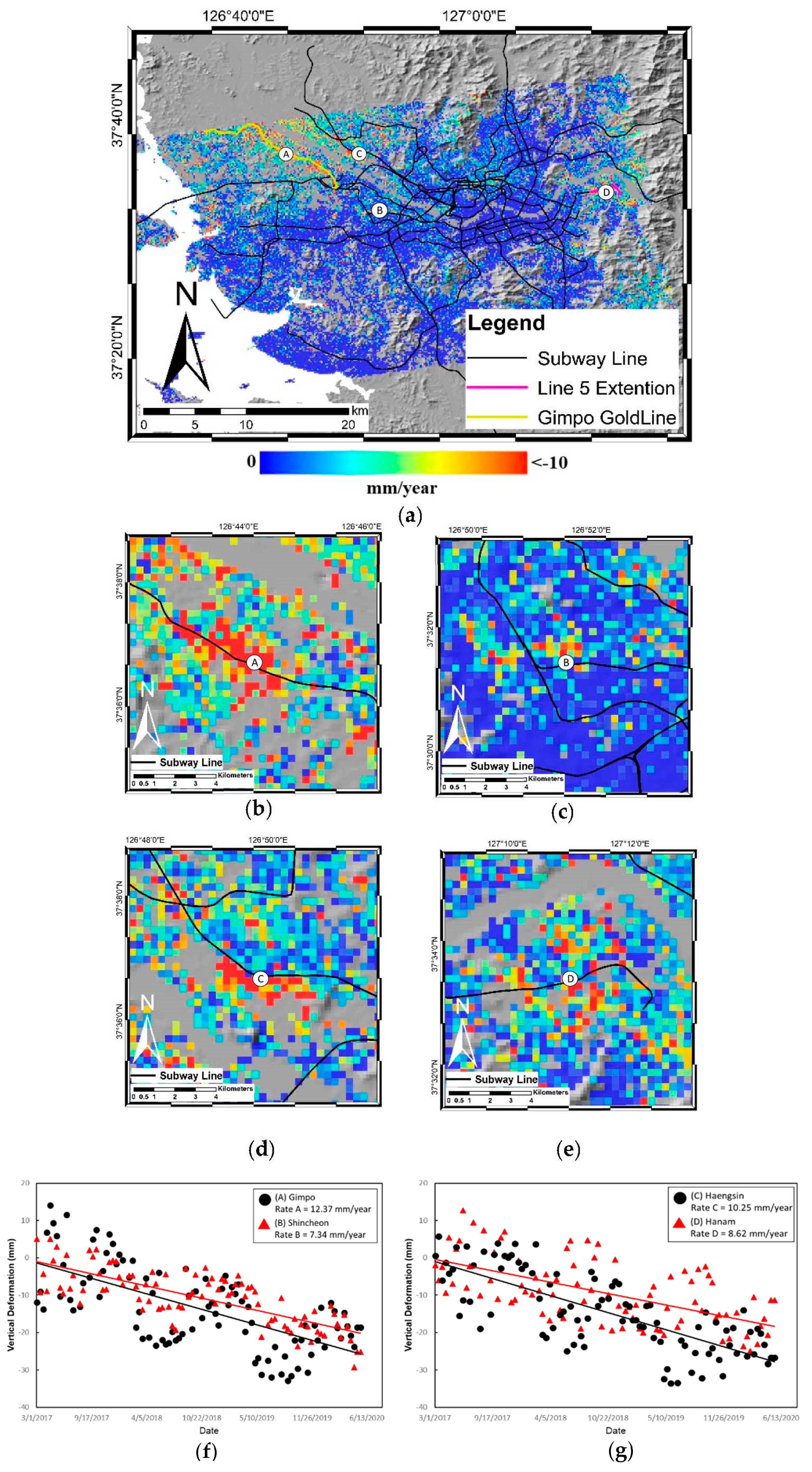
3.1. Land Subsidence Inventory Map

The land subsidence map from the Seoul Metropolitan Area was generated via the PSI-StaMPS method, using InSAR images in descending track captured from 2017 to 2020, and is shown in Figure 4a. To enhance measurement reliability, the vertical deformation map was generated using mean line-of-sight velocity [62]. Zooming locations for each selected point are shown in Figure 4b–e and the time-series graphs of all points are shown in Figure 4f,g.

In Figure 4b, represented the subsidence map in Gimpo the western part of this study area, with the black line indicating the subway line. In this area, especially in point A, there was a subsidence of 33.5 mm recorded with a mean deformation velocity of 12.57 mm/year from 2017 to 2020. The subsidence in Gimpo mostly occurs along the subway line that was newly operational in 2019. In this location, the subsidence is associated with the compressible deposits which consist of alluvium.

As can be seen from Figure 4c, the subsidence was exhibited around the subway line where the Shincheon subway station is located. Point B was recorded the maximum subsidence of up to 29 mm from 2017–2020 with the mean deformation velocity of 7.34 mm/year. This location consists of the intersection of subway line no 5 and subway line no 2, a residential area with high-density building also appears in this area. The subsidence in point B correlates with groundwater extraction and high-density building, as those conditions influence the subsidence rate in this area.

Figure 4d shows an overview of the subsidence near the Haengsin Station, known to be a depot for the metro train. The observation in point C revealed total subsidence of 34.35 mm from 2017 to 2020 and a mean deformation velocity of subsidence of 10.25 mm/year. The location is characterized by alluvium deposit that dominantly appears around the Han river. The geological features in this area show a correlation with the subsidence.

Figure 4e shows the subsidence map in Hanam city, the eastern part of the study area, with a black line indicates the subway line. The StaMPS result in point D shows the maximum subsidence of 26.17 mm from 2017 to 2020 with a mean deformation velocity rate of 8.42 mm/year. Hanam city is an area that has many developments such as residential areas and commercial buildings; subway construction is also being carried out in this area. Land subsidence can be related to underground work and building construction which pumping a large amount the groundwater [85]. In Hanam city, the subsidence is associated with urban land use and groundwater usage of this area.

Figure 4f,g show the time series graph from four selecting points in the study area. Generally, the periodic subsidence appeared in the vertical deformation graph. A possible reason for periodic subsidence in those areas was seasonal variation in the groundwater level and surface water loading. This result occurred due to the seasonal effect of groundwater extraction, where the selected points were surrounded by high-density buildings that mostly used groundwater as a water source. During the high season of groundwater withdrawal, the groundwater level decreased. After the rainy season, the groundwater level will rise and increase the aquifer system recovery (uplift) [84]. Those conditions may influence the deformation velocity in this study area.

3.2. Land Subsidence Susceptibility Map

Land subsidence susceptibility maps were constructed using the training dataset compiled from InSAR time-series data as land subsidence inventory map, ten land subsidence conditioning factors, and three different algorithms. Once the model training process was completed, susceptibility maps were constructed to visualize vulnerability to subsidence in the study area. In the land-subsidence-susceptibility map, each pixel in the study area was assigned a specific subsidence value using the quantile method [47].

Five susceptibility classes were used to reflect vulnerability to land subsidence: very low, low, moderate, high, and very high. Areas of very high susceptibility (marked red in Figure 5a–c) were most frequently found near the Han River and subway lines. The algorithms indicated that the northwestern area is very susceptible to subsidence, which may be due to several factors. For example, the geology of the northwestern area, which is near the Han River, is dominated by alluvium, which likely increases subsidence susceptibility. Most cases of observed subsidence have occurred on alluvium layers exhibiting natural consolidation; additionally, the increasing number of buildings and use of groundwater can exacerbate this condition [15,37,86]. A highly susceptible area was observed in the east, which may be associated with on-going construction in the same area. A few susceptible areas were observed along the northern Han River, mostly comprising high-density buildings and subway stations, but most of the northern area has low-to-moderate susceptibility to subsidence. Groundwater extraction in this area may increase the risk of subsidence, as some areas in which groundwater was extracted are now used for subway stations. Thus, the ground conditions in these areas might have been affected.

Figure 6 shows the distribution of pixels in each susceptibility map generated by the meta-ensemble models. In the land-subsidence-susceptibility map generated using the Bagging model, 63.67% of the area exhibited very low susceptibility to subsidence, whereas 15.53%, 7.55%, 6.42%, and 7.04% of the area exhibited low, moderate, high, and very high susceptibility to subsidence, respectively. In the map constructed using the Multiclass Classifier model, 63.66% and 18.31% of the area exhibited very low and low susceptibility to subsidence, respectively, whereas 10.98%, 1.62%, and 5.42% of the area exhibited moderate, high, and very high susceptibility to subsidence, respectively. Lastly, based on the LogitBoost model, most of the area was not very susceptible to subsidence, with 64.44%, 18.07%, 6.62%, 4.41%, and 6.66% of the map classified as areas of very low, low, moderate, high, and very high susceptibility, respectively. The distribution of pixels in very low class and very high class in Figure 6 has a similar pattern between each algorithm. A very high class can be considered as the subsidence area. Meanwhile, medium and high classes are considered as areas of future land subsidence and very low and low classes are areas with the lowest probability of land subsidence in the future. With this description, it is possible to know the area and the extent of the potential for subsidence that will occur in the future. Generally, the consistency of this model can be evaluated based on the presence of past land subsidence in land subsidence susceptibility classes. The existence of a higher percentage of land subsidence pixels in a higher degree of susceptibility classes indicates higher consistency and vice-versa.

3.3. Model Validation

A good land-subsidence-susceptibility map should be able to predict future subsidence in the target area and provide initial information for preventative actions. To validate our susceptibility maps, the accuracy of all used algorithms in this study was evaluated by ROC curve analysis. ROC curve analysis has been used as a standard way of validating the probability models used to generate land subsidence susceptibility maps, according to the area under the curve (AUC) [6]. The AUC, which ranges from 0.5 to 1, was used to assess model accuracy. An AUC value near 0.5 indicates that a model is inaccurate, whereas a value near 1.0 indicates an ideal model with a good fit [50]. AUCs were calculated to compare model performance, with the model with the highest AUC value was taken to be the best model. The Bagging model produced the largest AUC (0.883), followed by the LogitBoost model (0.871) and the Multiclass Classifier model (0.856) as shown in Figure 7. Thus, the Bagging model generated the best subsidence-susceptibility map in this study. However, all models produced good AUC values, indicating that they all performed well in terms of predicting land-subsidence susceptibility in the study area.

4. Discussion

4.1. Land Subsidence Inventory Map

StaMPS was employed to analyze land subsidence in the Seoul Metropolitan Area, with a deformation time-series map generated for all-terrain in the area based on descending-track data acquired from March 2017 to May 2020. Subsequently, a vertical deformation map was generated from the time-series analysis.

The results indicate that occurrences of subsidence were distributed over several locations in the study area, such as at Gimpo City (Figure 4a, point A). At this location, subsidence occurred near a new subway line that opened in 2019. Subsidence also occurred near a station with two subway lines near the southern Han River; high-density buildings are also found in this area (Figure 4a, point B). Other areas where subsidence occurred include a Seoul metro depot for several subway lines (Figure 4a, point C) and a newly developed area with several recently constructed residential and commercial buildings (Figure 4a, point D). Cases of land subsidence in the Seoul Metropolitan Area almost mostly occurred in the vicinity of subway lines or where the ground was weak. In particular, all areas of subsidence were located near subway lines and stations, implying that subway operation may be associated with subsidence in the study area [38,87]. Additionally, subway-tunnel excavations might have impacted the surrounding soil and the environment. During construction, how underground water is discharged, and the excavation method should be taken into consideration. Further analysis is needed to examine the impacts of construction on land subsidence in this area.

In terms of urbanization, the construction of buildings near subway lines and stations may add to the load on the soil and increase the risk of subsidence. High demand for transportation and urbanization increases the intensity of building construction and the amount of groundwater extracted. Besides, the groundwater extraction to fulfill social demand can influence the subsidence rate in the study area [3,88]. From the time-series deformation graph in Figure 4f, we can see a seasonal variation of subsidence rate in the study area between 2017–2020. It can also be noted that the high subsidence may appear in summer seasons. On the other hand, the subsidence rates lower after the rainy season which appears in July–August [3], the aquifer conditions after the rainy season are expected to have some influence on the subsidence rate. More study based on the water-level data analysis is required to better assess the possibility of the deformation, and further details of the structure and hydrologic parameters of groundwater should be resolved [89]. A combination of InSAR time-series analysis and analysis of hydrology of the area subsidence and the geomechanical parameters of the underlying aquifer structure area is a potential research topic to find out the cause of subsidence.

However, information extraction from the StaMPS technique is sometimes difficult due to a large number of PSs, thereby long interpretation times. The large amounts of PSs may cause several deficiencies in the analysis process, such as a reduction in the extraction of useful information from the dataset. Also, to obtain better time-series analysis results, several optimization steps can be taken for persistent scatterer points [20]. Several optimization methods for selecting PS points have been carried out [20,90]. This, in turn, could serve as a reference for future work on land subsidence studies that could increase efficiency and potentially lead to better deformation analyzes. Further studies should investigate other factors related to land subsidence. The results of GIS analysis are discussed below.

4.2. Land Subsidence Susceptibility Maps

Land subsidence should be mapped accurately to prepare subsidence inventories for target areas as an essential part of susceptibility analysis. To generate a subsidence-inventory map, we used InSAR remote-sensing data, which covered a broad area and were collected efficiently. Moreover, the InSAR time-series (StaMPS) method allows measuring of land subsidence and its rate to be measured to millimeter-level [37]. ArcGIS software was used for database construction, coordinate conversion, overlay analysis, and susceptibility modeling. Subsidence-related factors were identified based on information derived from the literature before susceptibility maps were generated [40,49]. Meta-ensemble machine learning was applied to estimate land-subsidence susceptibility, using three algorithms—Bagging, LogitBoost, and Multiclass Classifier.

Land subsidence susceptibility maps revealed that the northwestern and eastern areas, as well as a small area in the center, were most susceptible to land subsidence. We analyzed subsidence-related factors by comparing general patterns of subsidence with factor maps. The results revealed that most cases of subsidence occurred in areas where the ground consisted of alluvial layers, especially for subsidence that occurred near the Han River. However, there is a potential for subsidence in central areas that have different geological conditions from these two regions which are dominated by the alluvium layer. In this case, there are other factor influences besides geological factors in this subsidence modeling. The central area was assessed as moderately to highly susceptible to subsidence. In this area, there is a high density of buildings, and groundwater had been extracted at several spots near a subway station. Accordingly, groundwater outflow during subway operation could be another cause of land subsidence in this area [91]. If large amounts of groundwater are extracted, the surrounding soil structure may be affected. Thus, the weakened soil may be less able to withstand the pressure from aboveground buildings. Based on spatial distribution analysis, land use and groundwater extraction most strongly influence subsidence. In this study, the groundwater-extraction map was obtained via the interpolation of data on groundwater extraction near the subway infrastructure in Seoul, which might have generated errors in spatial distribution. Access to groundwater data for areas outside Seoul would allow for more accurate analyses of land subsidence.

In addition, several other factors that have not been identified in this study can be evaluated. The selection of these factors is based on the previous literature which may have some differences such as the condition of the area study and the subsidence mechanism. For this reason, additional analysis of factors related to the subsidence mechanism is needed to adjust to several concepts or assumptions of the subsidence mechanism that could potentially occur. However, adding some details such as aquifer conditions and groundwater levels can help evaluate the correlation of these factors and have the potential to improve the land subsidence susceptibility maps.

Susceptibility maps were validated based on ROC curves and AUC values and by comparing map predictions with testing data, which comprised 50% of the total dataset. The results indicate that the meta-ensemble approach performed better than the other approaches. A traditional model based on frequency ratio produced an AUC of 0.844, whereas the AUCs produced by the meta-ensemble models Multiclass Classifier, LogitBoost, and Bagging were 1.2%, 2.7%, and 2.95% larger, respectively. Therefore, these techniques can reduce bias and account for factor weights to improve the accuracy of predictions.

Although all models produced good AUC values and thus performed well in terms of predicting land subsidence in the study area, the susceptibility map constructed using the Bagging model was the most accurate. These results agree well with previous findings that model performance in terms of predicting subsidence improves with the use of machine learning [92]. Therefore, the Bagging model should be used for the susceptibility map. In fact, the Bagging model uses more recently well-organized techniques in soft computing modeling that not only enable improvement of a single classifier but can also deal with complex and high-dimensional modeling problems. Given the complexity of land subsidence and the interaction of several related factors, novel combinations of model-method can considerably improve the accuracy of land subsidence prediction.

5. Conclusions

This study aimed to assess and map land-subsidence susceptibility in the Seoul Metropolitan Area using InSAR data from Sentinel-1 acquired between 2017 and 2020. A deformation time-series map was generated using StaMPS, which revealed that land subsidence occurred in four areas (Figure 4a), with subsidence rates of 6–12 mm/year. Subsidence mostly occurred near subway lines and where a new subway line was being constructed. Besides, the subsidence occurrence in areas with high-density building and heavy groundwater extraction may lead to weakening of the ground.

To identify the factors influencing land subsidence, 10 potential subsidence-related factors were analyzed. Factor maps were overlaid with subsidence maps and each pixel within a layer was evaluated in a GIS environment. The training and testing datasets were prepared from time-series InSAR from the Sentinel-1 SAR dataset using the StaMPS method. Then, the spatial correlation for each factor was calculated using the frequency ratio. Meta-ensemble algorithms (Bagging, LogitBoost, and Multiclass Classifier) were employed to generate land-subsidence-susceptibility maps, and model performance in terms of reliability and prediction accuracy was compared using ROC analysis.

The land-subsidence-susceptibility maps revealed that the northwestern and eastern areas, as well as a small central area, were most vulnerable to land subsidence. The susceptibility of the northwestern and eastern areas most appear in the geological condition which is dominated by alluvium. By contrast, in the central area, which is moderate to highly susceptible, land use and groundwater extraction are the main factors influencing subsidence risk. From the ROC analysis, the AUC produced by each model was computed. All models performed well (AUC > 0.8). Bagging produced the largest AUC of 0.883, followed by LogitBoost (0.871) and Multiclass Classifier (0.856). Compared with the frequency-ratio method, machine-learning models produced more accurate predictions and are thus more appropriate for subsidence analysis in this study area.

Accurate predictions are essential for environmental planning to control and mitigate the impacts of land subsidence. Land-subsidence-susceptibility mapping is a valuable method for identifying areas with a high risk of land subsidence. Despite limitations associated with the datasets used in this study, we demonstrated that the analysis of remote-sensing and GIS spatial data via the machine-learning approach generates reliable and accurate predictions of land subsidence. Further research is needed to determine the effect of aquifer conditions, subway construction and operation on land subsidence. A large dataset of PS points may influence a deficiency in extracting useful information. The optimization approaches for selecting PS points must be proposed to overcome those limitations in future work such as optimization hotspot analysis and other statistic methods [20,90]. Furthermore, with the high complexity of the relationship between land subsidence and other factors, a novel combination of a machine learning and meta-heuristic algorithm as a hybrid method can improve the results of the land subsidence susceptibility map.

References

1. Machowski, R.; Rzetala, M.A.; Rzetala, M.; Solarski, M. Geomorphological and Hydrological Effects of Subsidence and Land use Change in Industrial and Urban Areas. Land Degrad. Dev. 2016, 27, 1740–1752. [Google Scholar] [CrossRef]
2. Jo, Y.-S.; Cho, S.-H.; Jang, Y.-S. Field investigation and analysis of ground sinking development in a metropolitan city, Seoul, Korea. Environ. Earth Sci. 2016, 75, 1353. [Google Scholar] [CrossRef]
3. Lee, H.; Oh, J. Establishing an ANN-based risk model for ground subsidence along railways. Appl. Sci. 2018, 8, 1936. [Google Scholar] [CrossRef] [Green Version]
4. Yuan, C.; Wang, X.; Wang, N.; Zhao, Q. Study on the Effect of Tunnel Excavation on Surface Subsidence Based on GIS Data Management. Procedia Environ. Sci. 2012, 12, 1387–1392. [Google Scholar] [CrossRef] [Green Version]
5. Roccheggiani, M.; Piacentini, D.; Tirincanti, E.; Perissin, D.; Menichetti, M. Detection and monitoring of tunneling induced ground movements using Sentinel-1 SAR interferometry. Remote Sens. 2019, 11, 639. [Google Scholar] [CrossRef] [Green Version]
6. Oh, H.J.; Lee, S. Assessment of ground subsidence using GIS and the weights-of-evidence model. Eng. Geol. 2010, 115, 36–48. [Google Scholar] [CrossRef]
7. Cigna, F.; Osmanoǧlu, B.; Cabral-Cano, E.; Dixon, T.H.; Ávila-Olivera, J.A.; Garduño-Monroy, V.H.; DeMets, C.; Wdowinski, S. Monitoring land subsidence and its induced geological hazard with Synthetic Aperture Radar Interferometry: A case study in Morelia, Mexico. Remote Sens. Environ. 2012, 117, 146–161. [Google Scholar] [CrossRef]
8. Chen, B.; Gong, H.; Chen, Y.; Li, X.; Zhou, C.; Lei, K.; Zhu, L.; Duan, L.; Zhao, X. Land subsidence and its relation with groundwater aquifers in Beijing Plain of China. Sci. Total Environ. 2020, 735, 139111. [Google Scholar] [CrossRef]
9. Amelung, F.; Galloway, D.L.; Bell, J.W.; Zebker, H.A.; Laczniak, R.J. Sensing the ups and downs of Las Vegas: InSAR reveals structural control of land subsidence and aquifer-system deformation. Geology 1999, 27, 483–486. [Google Scholar] [CrossRef]
10. Huang, Y.; Jiang, X. Field-observed phenomena of seismic liquefaction and subsidence during the 2008 Wenchuan earthquake in China. Nat. Hazards 2010, 54, 839–850. [Google Scholar] [CrossRef]
11. Osmanoǧlu, B.; Dixon, T.H.; Wdowinski, S.; Cabral-Cano, E.; Jiang, Y. Mexico City subsidence observed with persistent scatterer InSAR. Int. J. Appl. Earth Obs. Geoinf. 2011, 13, 1–12. [Google Scholar] [CrossRef]
12. Xu, Y.S.; Ma, L.; Shen, S.L.; Sun, W.J. Evaluation de la subsidence en considérant les structures constituant les aquifères de Shanghai, Chine. Hydrogeol. J. 2012, 20, 1623–1634. [Google Scholar] [CrossRef]
13. Ng, A.H.M.; Ge, L.; Li, X.; Abidin, H.Z.; Andreas, H.; Zhang, K. Mapping land subsidence in Jakarta, Indonesia using persistent scatterer interferometry (PSI) technique with ALOS PALSAR. Int. J. Appl. Earth Obs. Geoinf. 2012, 18, 232–242. [Google Scholar] [CrossRef]
14. Chaussard, E.; Amelung, F.; Abidin, H.; Hong, S.H. Sinking cities in Indonesia: ALOS PALSAR detects rapid subsidence due to groundwater and gas extraction. Remote Sens. Environ. 2013, 128, 150–161. [Google Scholar] [CrossRef]
15. Abidin, H.Z.; Djaja, R.; Darmawan, D.; Hadi, S.; Akbar, A.; Rajiyowiryono, H.; Sudibyo, Y.; Meilano, I.; Kasuma, M.A.; Kahar, J.; et al. Land subsidence of Jakarta (Indonesia) and its geodetic monitoring system. Nat. Hazards 2001, 23, 365–387. [Google Scholar] [CrossRef]
16. OECD. Health at a Glance 2013: OECD Indicators; OECD Publishing: Paris, France, 2013. [Google Scholar] [CrossRef] [Green Version]
17. Lee, J.Y.; Kwon, K.D.; Raza, M. Current water uses, related risks, and management options for Seoul megacity, Korea. Environ. Earth Sci. 2018, 77. [Google Scholar] [CrossRef]
18. Hanssen, R.F. Radar Interferometry: Data Interpretation and Error Analysis; Kluwer Academic: New York, NY, USA, 2010; ISBN 9789048156962. [Google Scholar]
19. Kang, Y.; Zhao, C.; Zhang, Q.; Lu, Z.; Li, B. Application of InSAR Techniques to an Analysis of the Guanling Landslide. Remote Sens. 2017, 9, 1046. [Google Scholar] [CrossRef] [Green Version]
20. Lu, P.; Bai, S.; Tofani, V.; Casagli, N. Landslides detection through optimized hot spot analysis on persistent scatterers and distributed scatterers. ISPRS J. Photogramm. Remote Sens. 2019, 156, 147–159. [Google Scholar] [CrossRef]
21. Perissin, D.; Ferretti, A. Urban-target recognition by means of repeated spaceborne SAR images. IEEE Trans. Geosci. Remote Sens. 2007, 45, 4043–4058. [Google Scholar] [CrossRef]
22. Motagh, M.; Shamshiri, R.; Haghshenas Haghighi, M.; Wetzel, H.U.; Akbari, B.; Nahavandchi, H.; Roessner, S.; Arabi, S. Quantifying groundwater exploitation induced subsidence in the Rafsanjan plain, southeastern Iran, using InSAR time-series and in situ measurements. Eng. Geol. 2017, 218, 134–151. [Google Scholar] [CrossRef]
23. Aly, M.H.; Klein, A.G.; Zebker, H.A.; Giardino, J.R. Land subsidence in the Nile Delta of Egypt observed by persistent scatterer interferometry. Remote Sens. Lett. 2012, 3, 621–630. [Google Scholar] [CrossRef]
24. Crosetto, M.; Monserrat, O.; Cuevas-González, M.; Devanthéry, N.; Crippa, B. Persistent Scatterer Interferometry: A review. ISPRS J. Photogramm. Remote Sens. 2016, 115, 78–89. [Google Scholar] [CrossRef] [Green Version]
25. Riddick, S.N.; Schmidt, D.A.; Deligne, N.I. An analysis of terrain properties and the location of surface scatterers from persistent scatterer interferometry. ISPRS J. Photogramm. Remote Sens. 2012, 73, 50–57. [Google Scholar] [CrossRef]
26. Khorrami, M.; Abrishami, S.; Maghsoudi, Y.; Alizadeh, B.; Perissin, D. Extreme subsidence in a populated city (Mashhad) detected by PSInSAR considering groundwater withdrawal and geotechnical properties. Sci. Rep. 2020, 10, 1–16. [Google Scholar] [CrossRef] [PubMed]
27. Yazici, B.V.; Tunc Gormus, E. Investigating persistent scatterer InSAR (PSInSAR) technique efficiency for landslides mapping: A case study in Artvin dam area, in Turkey. Geocarto Int. 2020, 1–19. [Google Scholar] [CrossRef]
28. Jiaxuan, H.; Mowen, X.; Atkinson, P.M. Dynamic susceptibility mapping of slow-moving landslides using PSInSAR. Int. J. Remote Sens. 2020, 41, 7509–7529. [Google Scholar] [CrossRef]
29. Tessitore, S.; Fernández-Merodo, J.A.; Herrera, G.; Tomás, R.; Ramondini, M.; Sanabria, M.; Duro, J.; Mulas, J.; Calcaterra, D. Comparison of water-level, extensometric, DInSAR and simulation data for quantification of subsidence in Murcia City (SE Spain). Hydrogeol. J. 2016, 24, 727–747. [Google Scholar] [CrossRef]
30. Wang, H.; Feng, G.; Xu, B.; Yu, Y.; Li, Z.; Du, Y.; Zhu, J. Deriving spatio-temporal development of ground subsidence due to subway construction and operation in Delta regions with PS-InSAR data: A case study in Guangzhou, China. Remote Sens. 2017, 9, 1004. [Google Scholar] [CrossRef] [Green Version]
31. Khakim, M.Y.N.; Tsuji, T.; Matsuoka, T. Lithology-controlled subsidence and seasonal aquifer response in the Bandung basin, Indonesia, observed by synthetic aperture radar interferometry. Int. J. Appl. Earth Obs. Geoinf. 2014, 32, 199–207. [Google Scholar] [CrossRef] [Green Version]
32. Zhou, C.; Gong, H.; Chen, B.; Gao, M.; Cao, Q.; Cao, J.; Duan, L.; Zuo, J.; Shi, M. Land Subsidence Response to Different Land Use Types and Water Resource Utilization in Beijing-Tianjin-Hebei, China. Remote Sens. 2020, 12, 457. [Google Scholar] [CrossRef] [Green Version]
33. Lu, P.; Han, J.; Hao, T.; Li, R.; Qiao, G. Seasonal Deformation of Permafrost in Wudaoliang Basin in Qinghai-Tibet Plateau Revealed by StaMPS-InSAR. Mar. Geod. 2020, 43, 248–268. [Google Scholar] [CrossRef]
34. Jennifer, J.J.; Saravanan, S.; Pradhan, B. Persistent Scatterer Interferometry in the post-event monitoring of the Idukki Landslides. Geocarto Int. 2020. [Google Scholar] [CrossRef]
35. Tzampoglou, P.; Loupasakis, C. Mining geohazards susceptibility and risk mapping: The case of the Amyntaio open-pit coal mine, West Macedonia, Greece. Environ. Earth Sci. 2017, 76. [Google Scholar] [CrossRef]
36. Tofani, V.; Raspini, F.; Catani, F.; Casagli, N. Persistent Scatterer Interferometry (PSI) Technique for Landslide Characterization and Monitoring. Remote Sens. 2013, 5, 1045–1065. [Google Scholar] [CrossRef] [Green Version]
37. Bianchini, S.; Solari, L.; Del Soldato, M.; Raspini, F.; Montalti, R.; Ciampalini, A.; Casagli, N. Ground Subsidence Susceptibility (GSS) Mapping in Grosseto Plain (Tuscany, Italy) Based on Satellite InSAR Data Using Frequency Ratio and Fuzzy Logic. Remote Sens. 2019, 11, 2015. [Google Scholar] [CrossRef] [Green Version]
38. Ng, A.H.M.; Wang, H.; Dai, Y.; Pagli, C.; Chen, W.; Ge, L.; Du, Z.; Zhang, K. InSAR reveals land deformation at Guangzhou and Foshan, China between 2011 and 2017 with COSMO-SkyMed data. Remote Sens. 2018, 10, 813. [Google Scholar] [CrossRef] [Green Version]
39. Lan, H.X.; Zhou, C.H.; Wang, L.J.; Zhang, H.Y.; Li, R.H. Landslide hazard spatial analysis and prediction using GIS in the Xiaojiang watershed, Yunnan, China. Eng. Geol. 2004, 76, 109–128. [Google Scholar] [CrossRef]
40. Pradhan, B.; Abokharima, M.H.; Jebur, M.N.; Tehrany, M.S. Land subsidence susceptibility mapping at Kinta Valley (Malaysia) using the evidential belief function model in GIS. Nat. Hazards 2014, 73, 1019–1042. [Google Scholar] [CrossRef]
41. Regmi, A.D.; Yoshida, K.; Nagata, H.; Pradhan, A.M.S.; Pradhan, B.; Pourghasemi, H.R. The relationship between geology and rock weathering on the rock instability along Mugling-Narayanghat road corridor, Central Nepal Himalaya. Nat. Hazards 2013, 66, 501–532. [Google Scholar] [CrossRef]
42. Lee, S.; Park, I.; Choi, J.K. Spatial prediction of ground subsidence susceptibility using an artificial neural network. Environ. Manag. 2012, 49, 347–358. [Google Scholar] [CrossRef]
43. Arabameri, A.; Saha, S.; Roy, J.; Tiefenbacher, J.P.; Cerda, A.; Biggs, T.; Pradhan, B.; Thi Ngo, P.T.; Collins, A.L. A novel ensemble computational intelligence approach for the spatial prediction of land subsidence susceptibility. Sci. Total Environ. 2020, 726, 138595. [Google Scholar] [CrossRef] [PubMed]
44. Pradhan, B. A comparative study on the predictive ability of the decision tree, support vector machine and neuro-fuzzy models in landslide susceptibility mapping using GIS. Comput. Geosci. 2013, 51, 350–365. [Google Scholar] [CrossRef]
45. Wu, W.; Zucca, C.; Karam, F.; Liu, G. Enhancing the performance of regional land cover mapping. Int. J. Appl. Earth Obs. Geoinf. 2016, 52, 422–432. [Google Scholar] [CrossRef]
46. Tien Bui, D.; Ho, T.C.; Revhaug, I.; Pradhan, B.; Nguyen, D.B. Landslide Susceptibility Mapping Along the National Road 32 of Vietnam Using GIS-Based J48 Decision Tree Classifier and Its Ensembles. In Cartography from Pole to Pole; Springer: Berlin/Heidelberg, Germany, 2014; pp. 303–317. [Google Scholar]
47. Kadavi, P.R.; Lee, C.W.; Lee, S. Application of ensemble-based machine learning models to landslide susceptibility mapping. Remote Sens. 2018, 10, 1252. [Google Scholar] [CrossRef] [Green Version]
48. Hong, H.; Liu, J.; Zhu, A.X. Modeling landslide susceptibility using LogitBoost alternating decision trees and forest by penalizing attributes with the bagging ensemble. Sci. Total Environ. 2020, 718, 137231. [Google Scholar] [CrossRef] [PubMed]
49. Abdollahi, S.; Pourghasemi, H.R.; Ghanbarian, G.A.; Safaeian, R. Prioritization of effective factors in the occurrence of land subsidence and its susceptibility mapping using an SVM model and their different kernel functions. Bull. Eng. Geol. Environ. 2019, 78, 4017–4034. [Google Scholar] [CrossRef]
50. Fawcett, T. An introduction to ROC analysis. Pattern Recognit. Lett. 2006, 27, 861–874. [Google Scholar] [CrossRef]
51. Kim, Y.Y.; Lee, K.K.; Sung, I.H. Urbanization and the groundwater budget, metropolitan Seoul area, Korea. Hydrogeol. J. 2001, 9, 401–412. [Google Scholar] [CrossRef]
52. Korea, S. Complete Enumeration Results of the 2010 Population and Housing Census; Statistics Korea: Daejeon, Korea, 2011. [Google Scholar]
53. Choi, B.Y.; Yun, S.T.; Yu, S.Y.; Lee, P.K.; Park, S.S.; Chae, G.T.; Mayer, B. Hydrochemistry of urban groundwater in Seoul, South Korea: Effects of land-use and pollutant recharge. Environ. Geol. 2005, 48, 979–990. [Google Scholar] [CrossRef]
54. Chae, G.T.; Yun, S.T.; Kim, D.S.; Kim, K.H.; Joo, Y. Time-series analysis of three years of groundwater level data (Seoul, South Korea) to characterize urban groundwater recharge. Q. J. Eng. Geol. Hydrogeol. 2010, 43, 117–127. [Google Scholar] [CrossRef]
55. Korea, R. KORAIL Sustainability Report 2015; Korea Railroad Corporation: Daejeon, Korea, 2015. [Google Scholar]
56. Farr, T.G.; Rosen, P.A.; Caro, E.; Crippen, R.; Duren, R.; Hensley, S.; Kobrick, M.; Paller, M.; Rodriguez, E.; Roth, L.; et al. The shuttle radar topography mission. Rev. Geophys. 2007, 45. [Google Scholar] [CrossRef] [Green Version]
57. Hooper, A.; Segall, P.; Zebker, H. Persistent scatterer interferometric synthetic aperture radar for crustal deformation analysis, with application to Volcán Alcedo, Galápagos. J. Geophys. Res. Solid Earth 2007, 112. [Google Scholar] [CrossRef] [Green Version]
58. Hooper, A.J. A multi-temporal InSAR method incorporating both persistent scatterer and small baseline approaches. Geophys. Res. Lett. 2008, 35. [Google Scholar] [CrossRef] [Green Version]
59. Sousa, J.J.; Hooper, A.J.; Hanssen, R.F.; Bastos, L.C.; Ruiz, A.M. Persistent Scatterer InSAR: A comparison of methodologies based on a model of temporal deformation vs. spatial correlation selection criteria. Remote Sens. Environ. 2011, 115, 2652–2663. [Google Scholar] [CrossRef]
60. Pepe, A.; Bonano, M.; Zhao, Q.; Yang, T.; Wang, H. The Use of C-/X-Band Time-Gapped SAR Data and Geotechnical Models for the Study of Shanghai’s Ocean-Reclaimed Lands through the SBAS-DInSAR Technique. Remote Sens. 2016, 8, 911. [Google Scholar] [CrossRef] [Green Version]
61. Ren, H.; Feng, X. Calculating vertical deformation using a single InSAR pair based on singular value decomposition in mining areas. Int. J. Appl. Earth Obs. Geoinf. 2020, 92, 102115. [Google Scholar] [CrossRef]
62. Yastika, P.; Shimizu, N.; Abidin, H.Z. Monitoring of long-term land subsidence from 2003 to 2017 in coastal area of Semarang, Indonesia by SBAS DInSAR analyses using Envisat-ASAR, ALOS-PALSAR, and Sentinel-1A SAR data. Adv. Space Res. 2019, 63, 1719–1736. [Google Scholar] [CrossRef]
63. Lee, S.; Park, I. Application of decision tree model for the ground subsidence hazard mapping near abandoned underground coal mines. J. Environ. Manag. 2013, 127, 166–176. [Google Scholar] [CrossRef]
64. Korjus, K.; Hebart, M.N.; Vicente, R. An Efficient Data Partitioning to Improve Classification Performance While Keeping Parameters Interpretable. PLoS ONE 2016, 11, e0161788. [Google Scholar] [CrossRef] [Green Version]
65. Jaafari, A.; Zenner, E.K.; Panahi, M.; Shahabi, H. Hybrid artificial intelligence models based on a neuro-fuzzy system and metaheuristic optimization algorithms for spatial prediction of wildfire probability. Agric. For. Meteorol. 2019, 266–267, 198–207. [Google Scholar] [CrossRef]
66. Kim, K.D.; Lee, S.; Oh, H.J.; Choi, J.K.; Won, J.S. Assessment of ground subsidence hazard near an abandoned underground coal mine using GIS. Environ. Geol. 2006, 50, 1183–1191. [Google Scholar] [CrossRef]
67. Silalahi, F.E.S.; Arifianti, Y.; Hidayat, F. Landslide susceptibility assessment using frequency ratio model in Bogor, West Java, Indonesia. Geosci. Lett. 2019, 6, 1–17. [Google Scholar] [CrossRef] [Green Version]
68. Breiman, L. Bagging predictors. Mach. Learn. 1996, 24, 123–140. [Google Scholar] [CrossRef] [Green Version]
69. Sedano, J.; Gonzalez, S.; Herrero, A.; Baruque, B.; Corchado, E. Mutating network scans for the assessment of supervised classifier ensembles. Log. J. IGPL 2013, 21, 630–647. [Google Scholar] [CrossRef] [Green Version]
70. Friedman, J.; Hastie, T.; Tibshirani, R. Additive logistic regression: A statistical view of boosting. Ann. Stat. 2000, 28, 337–407. [Google Scholar] [CrossRef]
71. Pourghasemi, H.; Gayen, A.; Park, S.; Lee, C.-W.; Lee, S. Assessment of Landslide-Prone Areas and Their Zonation Using Logistic Regression, LogitBoost, and NaïveBayes Machine-Learning Algorithms. Sustainability 2018, 10, 3697. [Google Scholar] [CrossRef] [Green Version]
72. Cai, Y.D.; Feng, K.Y.; Lu, W.C.; Chou, K.C. Using LogitBoost classifier to predict protein structural classes. J. Theor. Biol. 2006, 238, 172–176. [Google Scholar] [CrossRef] [PubMed]
73. Kowsari, K.; Brown, D.E.; Heidarysafa, M.; Meimandi, K.J.; Gerber, M.S.; Barnes, L.E. HDLTex: Hierarchical Deep Learning for Text Classification. In Proceedings of the 16th IEEE International Conference on Machine Learning and Applications, ICMLA 2017, Cancun, Mexico, 18–21 December 2017; Institute of Electrical and Electronics Engineers Inc.: Piscataway, NJ, USA, 2017; pp. 364–371. [Google Scholar]
74. Gambolati, G.; Teatini, P. Geomechanics of subsurface water withdrawal and injection. Water Resour. Res. 2015, 51, 3922–3955. [Google Scholar] [CrossRef]
75. Erban, L.E.; Gorelick, S.M.; Zebker, H.A. Groundwater extraction, land subsidence, and sea-level rise in the Mekong Delta, Vietnam. Environ. Res. Lett. 2014, 9, 084010. [Google Scholar] [CrossRef]
76. Suh, J.; Choi, Y.; Park, H.D. GIS-based evaluation of mining-induced subsidence susceptibility considering 3D multiple mine drifts and estimated mined panels. Environ. Earth Sci. 2016, 75, 1–19. [Google Scholar] [CrossRef]
77. Kim, K.; Kim, J.; Kwak, T.Y.; Chung, C.K. Logistic regression model for sinkhole susceptibility due to damaged sewer pipes. Nat. Hazards 2018, 93, 765–785. [Google Scholar] [CrossRef]
78. Del Giudice, G.; Padulano, R.; Siciliano, D. Multivariate probability distribution for sewer system vulnerability assessment under data-limited conditions. Water Sci. Technol. 2016, 73, 751–760. [Google Scholar] [CrossRef] [PubMed]
79. Yesilnacar, E.; Topal, T. Landslide susceptibility mapping: A comparison of logistic regression and neural networks methods in a medium scale study, Hendek region (Turkey). Eng. Geol. 2005, 79, 251–266. [Google Scholar] [CrossRef]
80. Andaryani, S.; Nourani, V.; Trolle, D.; Dehgani, M.; Asl, A.M. Assessment of land use and climate change effects on land subsidence using a hydrological model and radar technique. J. Hydrol. 2019, 578, 124070. [Google Scholar] [CrossRef]
81. Minderhoud, P.S.J.; Coumou, L.; Erban, L.E.; Middelkoop, H.; Stouthamer, E.; Addink, E.A. The relation between land use and subsidence in the Vietnamese Mekong delta. Sci. Total Environ. 2018, 634, 715–726. [Google Scholar] [CrossRef]
82. Yoo, C. Ground settlement during tunneling in groundwater drawdown environment—Influencing factors. Undergr. Space 2016, 1, 20–29. [Google Scholar] [CrossRef] [Green Version]
83. Arabameri, A.; Lee, S.; Tiefenbacher, J.P.; Ngo, P.T.T. Novel Ensemble of MCDM-Artificial Intelligence Techniques for Groundwater-Potential Mapping in Arid and Semi-Arid Regions (Iran). Remote Sens. 2020, 12, 490. [Google Scholar] [CrossRef] [Green Version]
84. Bell, J.W.; Amelung, F.; Ferretti, A.; Bianchi, M.; Novali, F. Permanent scatterer InSAR reveals seasonal and long-term aquifer-system response to groundwater pumping and artificial recharge. Water Resour. Res. 2008, 44. [Google Scholar] [CrossRef] [Green Version]
85. Lee, J.Y. Lessons from three groundwater disputes in Korea: Lack of comprehensive and integrated investigation. Int. J. Water 2017, 11, 59–72. [Google Scholar] [CrossRef]
86. Notti, D.; Mateos, R.M.; Monserrat, O.; Devanthéry, N.; Peinado, T.; Roldán, F.J.; Fernández-Chacón, F.; Galve, J.P.; Lamas, F.; Azañón, J.M. Lithological control of land subsidence induced by groundwater withdrawal in new urban AREAS (Granada Basin, SE Spain). Multiband DInSAR monitoring. Hydrol. Process. 2016, 30, 2317–2331. [Google Scholar] [CrossRef]
87. Chen, W.F.; Gong, H.L.; Chen, B.B.; Liu, K.S.; Gao, M.; Zhou, C.F. Spatiotemporal evolution of land subsidence around a subway using InSAR time-series and the entropy method. GISci. Remote Sens. 2017, 54, 78–94. [Google Scholar] [CrossRef]
88. Reeves, J.A.; Knight, R.; Zebker, H.A.; Kitanidis, P.K.; Schreüder, W.A. Estimating temporal changes in hydraulic head using InSAR data in the San Luis Valley, Colorado. Water Resour. Res. 2014, 50, 4459–4473. [Google Scholar] [CrossRef]
89. Motagh, M.; Walter, T.R.; Sharifi, M.A.; Fielding, E.; Schenk, A.; Anderssohn, J.; Zschau, J. Land subsidence in Iran caused by widespread water reservoir overexploitation. Geophys. Res. Lett. 2008, 35. [Google Scholar] [CrossRef] [Green Version]
90. Lu, P.; Casagli, N.; Catani, F.; Tofani, V. Persistent scatterers interferometry hotspot and cluster analysis (PSI-HCA) for detection of extremely slow-moving landslides. Int. J. Remote Sens. 2012, 33, 466–489. [Google Scholar] [CrossRef]
91. Seong, J.-H. The Contiguity Ground and Structures Sinkage Analysis of in City Excavation; Korean Geotechnical Society: Seoul, Korea, 2009. [Google Scholar]
92. Rahmati, O.; Golkarian, A.; Biggs, T.; Keesstra, S.; Mohammadi, F.; Daliakopoulos, I.N. Land subsidence hazard modeling: Machine learning to identify predictors and the role of human activities. J. Environ. Manag. 2019, 236, 466–480. [Google Scholar] [CrossRef]
Figure 1. Optical image of Seoul (gray) captured by Sentinel-2 on 19 June 2019 with subway lines superimposed.
Remotesensing 12 03505 g001
Figure 2. The workflow illustration.
Remotesensing 12 03505 g002
Figure 3. Train-test data point and spatial maps of 10 land-subsidence-related factor: train-test data point (a), elevation (b), slope (c), aspect (d), topographic wetness index (TWI) (e), profile curvature (f), land use (g), groundwater extraction (h), distance to river (i), lithology (j), and distance to fault (k).
Remotesensing 12 03505 g003aRemotesensing 12 03505 g003b
Figure 4. (a) Mean vertical deformation map in descending track of the Seoul Metropolitan Area generated from a Hillshade image comprising digital elevation model data from the Shuttle Radar Topography Mission. (b) Zooming of vertical deformation map at points A (Gimpo), (c) point B (Shincheon), (d) points C (Haengsin) and (e) points D (Hanam), (f) Vertical deformation time-series at points A (Gimpo) and B (Shincheon), and (g) points C (Haengsin) and D (Hanam).
Remotesensing 12 03505 g004
Figure 5. Land-subsidence-susceptibility map generated using three algorithms: the (a) Bagging, (b) LogitBoost, and (c) Multiclass Classifier algorithms.
Remotesensing 12 03505 g005
Figure 6. Distribution of pixels classified as areas of very low, low, moderate, high, and very high susceptibility in the land-subsidence-susceptibility maps generated by three machine-learning algorithms.
Remotesensing 12 03505 g006
Figure 7. Receiver operating characteristic (ROC) curves associated with land-subsidence-susceptibility maps generated by three meta-ensemble algorithms (Bagging, LogitBoost, and Multiclass Classifier).
Remotesensing 12 03505 g007