Land Subsidence Susceptibility Mapping in Jakarta Using Functional and Meta-Ensemble Machine Learning Algorithm Based on Time-Series InSAR Data


Abstract
:
1. Introduction
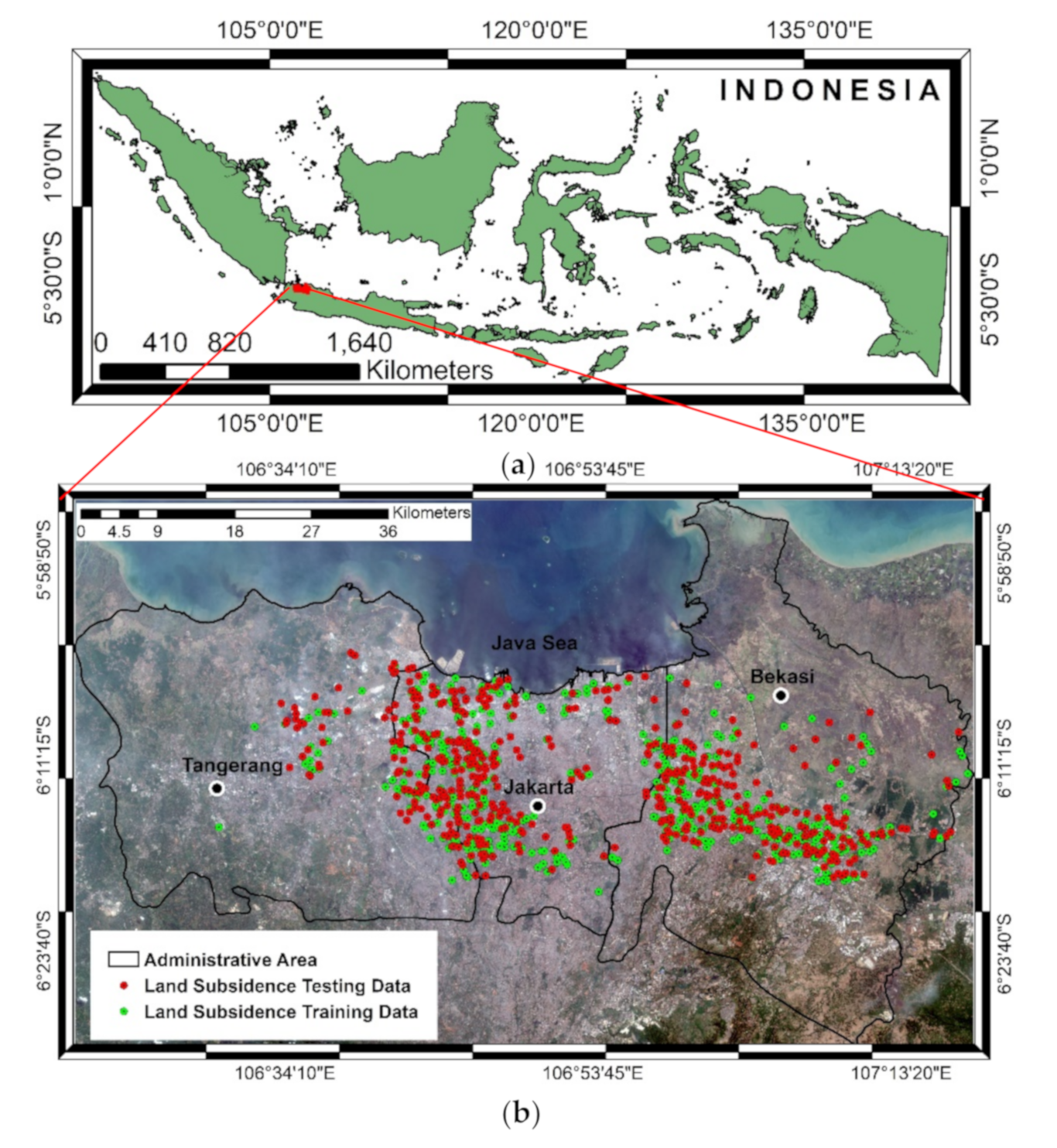
2. Study Area
3. Material and Methods
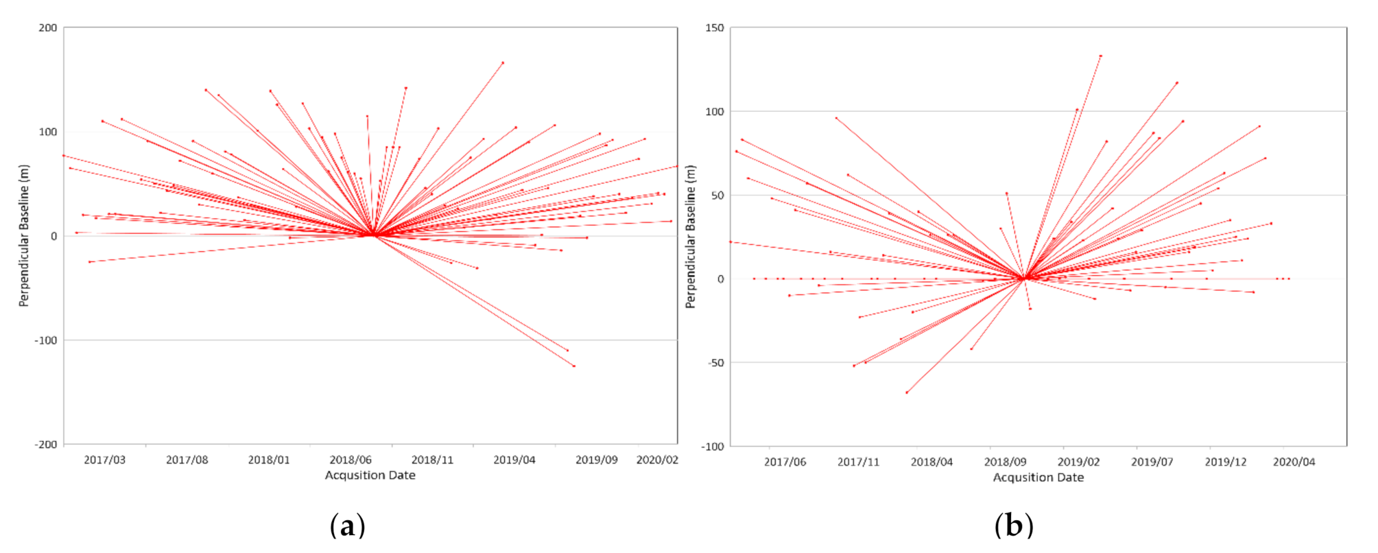
3.1. SAR Datasets
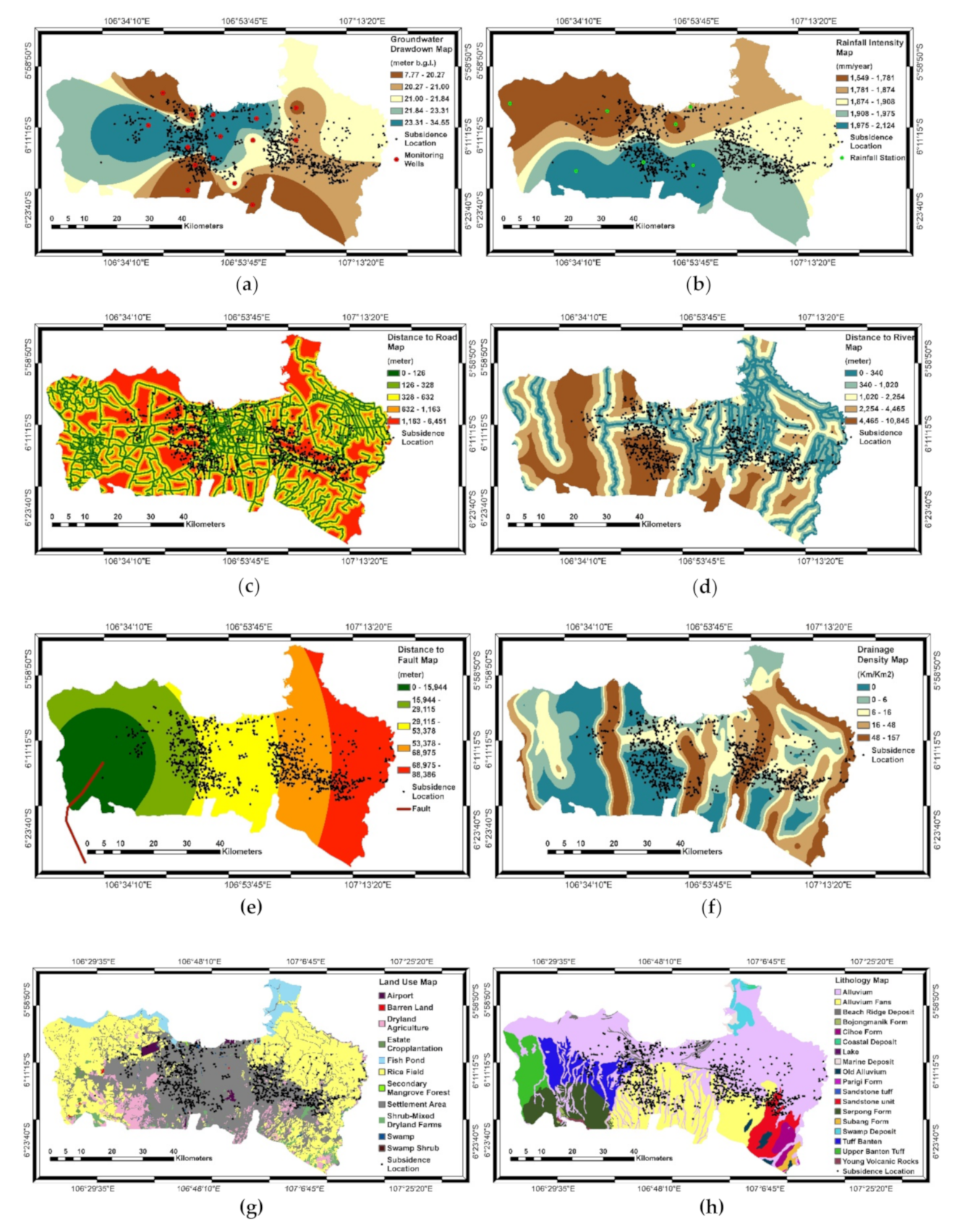
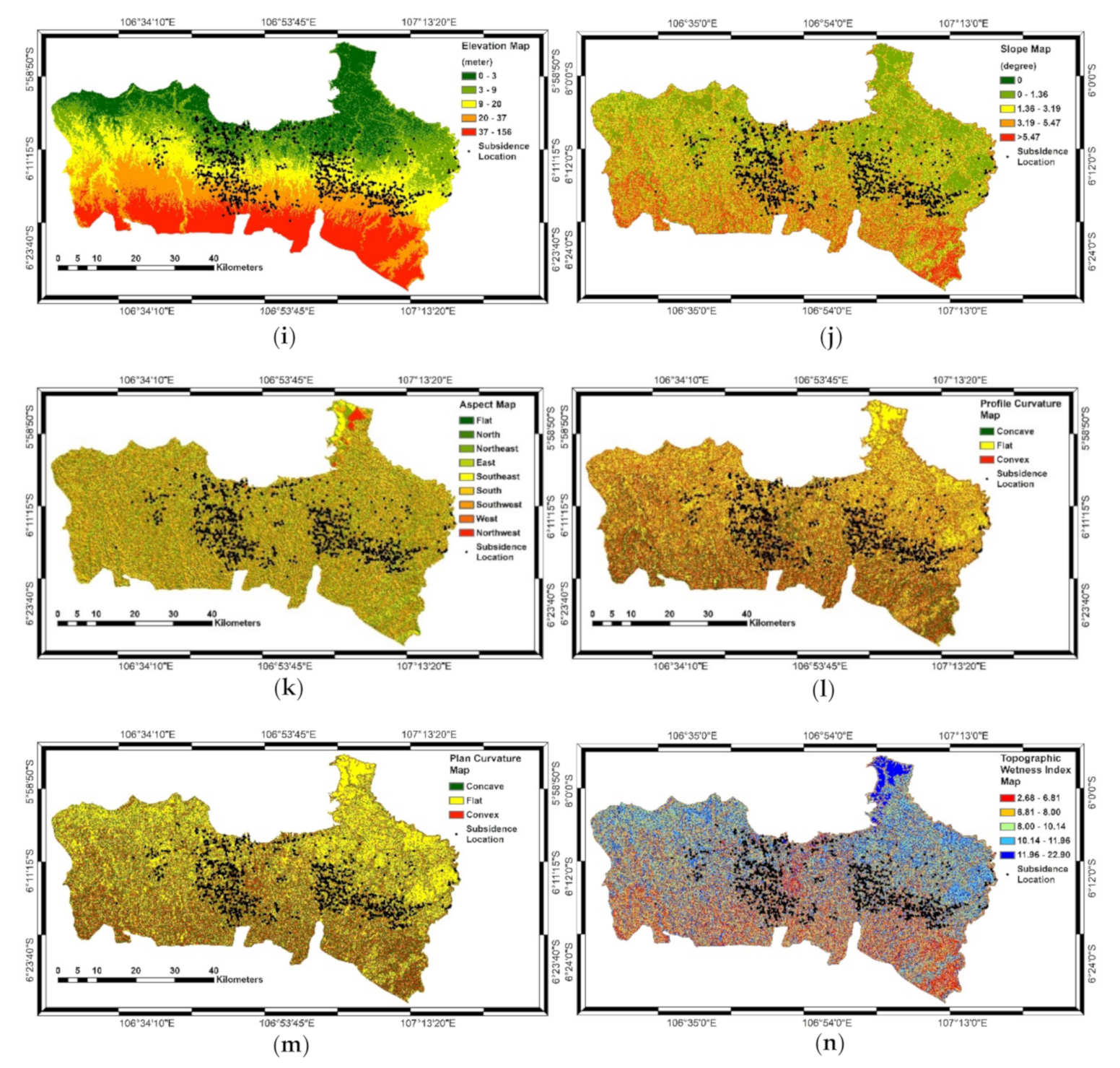
3.2. Land Subsidence Conditioning Factors
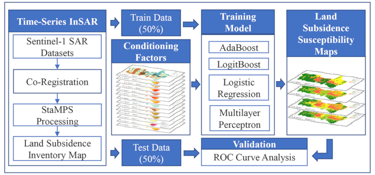
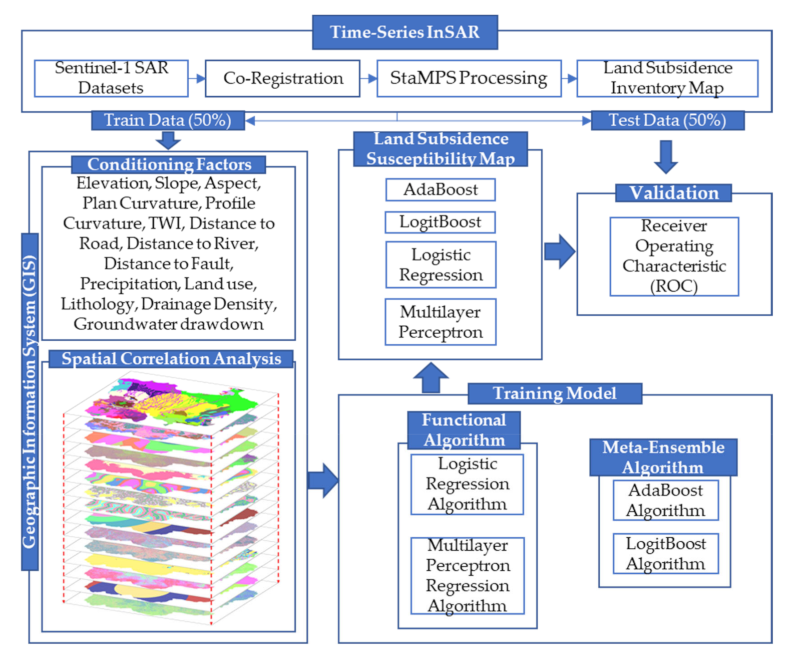
3.3. Illustration of Methodology
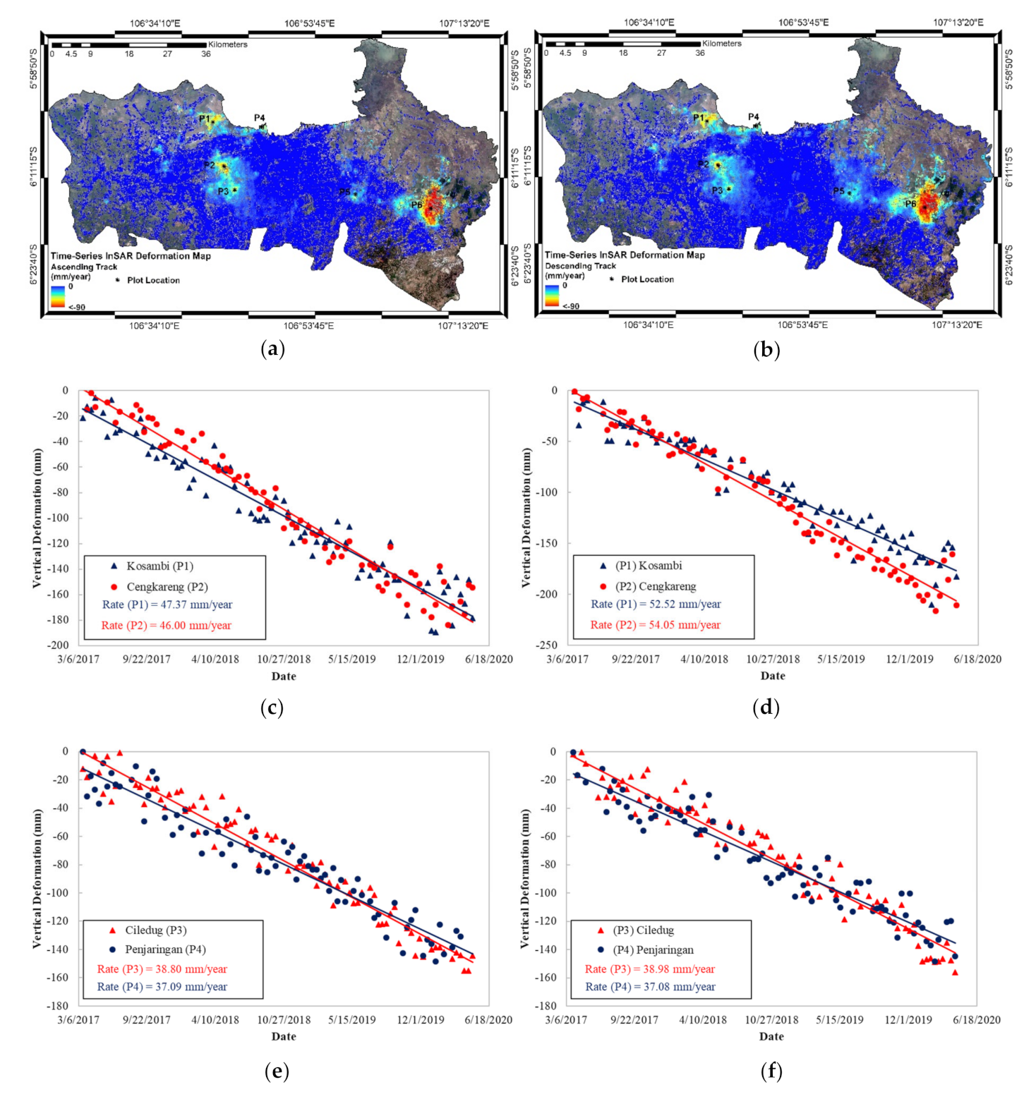
- Land subsidence occurrences were identified by exploiting Sentinel-1 SAR datasets from 2017 to 2020 from both ascending and descending tracks using time-series InSAR techniques based on the StaMPS algorithm. The persistent scatterer points from co-registered single master images showing a deformation value were used as the land subsidence inventory map.
- Preparation of training and testing datasets was conducted by randomly dividing the persistent scatterer (PS) points of time-series InSAR showing a vertical deformation into 50% training data to generate land subsidence susceptibility models and 50% testing data to validate the land subsidence susceptibility map, as done in other studies finding optimal results [28,53]. The distribution of training and test data is shown in Figure 1b.
- Preparation of land subsidence conditioning factors for spatial correlation analysis was done using the frequency ratio method to find the correlation between each factor and land subsidence occurrence [53]. We used each model’s ratio value and then used as the conditioning factors related to land subsidence occurrences. First, the conditioning factors were classified using quantile methods in GIS tools with a similar environment of 30 m cell size for each factor; then, the number of subsidence occurrences in each class was calculated using the cross-tabulation tool in GIS. Next, we calculated the ratio between the percentage of pixels of each conditioning factor class and the percentage of subsidence occurrence pixels to obtain the FR value as follows:
- 4.
- The conditioning factors consisting of frequency ratio values were used to generate land subsidence susceptibility models using two functional algorithms (logistic regression and multilayer perceptron) and two meta-ensemble algorithms (AdaBoost and LogitBoost).
- 5.
- After all land subsidence susceptibility maps were generated, all maps were validated using the test data prepared before and analyzed using ROC curve analysis.
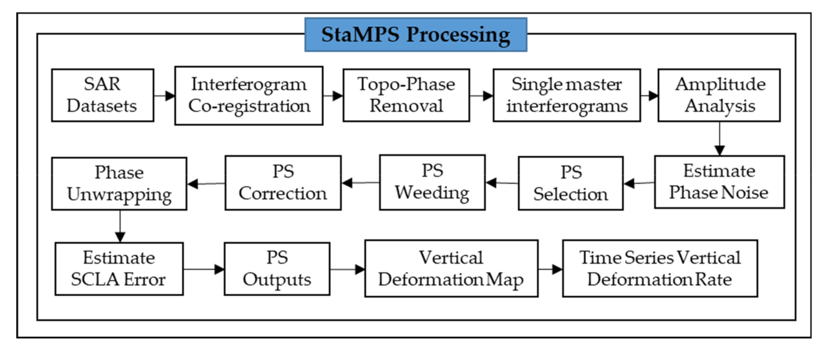
3.4. StaMPS Processing
3.5. AdaBoost
- Start with weights for
- Repeat this step for
- Fit the classifier using weights with the training data;
- Compute
- Set , and renormalize so that
- Output the classifier: .
3.6. LogitBoost
- Start with weights for , and probability estimates ;
- Repeat this step for
- Compute the working response and weights:
- Fit the function by weighted least-squares regression of to using weight
- Update the function as follows:
- Output the classifier: .
3.7. Logistic Regression
3.8. Multilayer Perceptron
4. Results
4.1. Land Subsidence Inventory Map
4.2. Land Subsidence Susceptibility Map
4.3. Model Validation
5. Discussion
5.1. Land Subsidence Inventory Map
5.2. Land Subsidence Susceptibility Map
6. Conclusions
Author Contributions
Funding
Conflicts of Interest
References
- Chaussard, E.; Amelung, F.; Abidin, H.; Hong, S.-H. Sinking cities in Indonesia: ALOS PALSAR detects rapid subsidence due to groundwater and gas extraction. Remote Sens. Environ. 2013, 128, 150–161. [Google Scholar] [CrossRef]
- Machowski, R.; Rzetala, M.A.; Rzetala, M.; Solarski, M. Geomorphological and Hydrological Effects of Subsidence and Land use Change in Industrial and Urban Areas. Land Degrad. Dev. 2016, 27, 1740–1752. [Google Scholar] [CrossRef]
- Abidin, H.Z.; Andreas, H.; Gumilar, I.; Fukuda, Y.; Pohan, Y.E.; Deguchi, T. Land subsidence of Jakarta (Indonesia) and its relation with urban development. Nat. Hazards 2011, 59, 1753–1771. [Google Scholar] [CrossRef]
- Takagi, H.; Esteban, M.; Mikami, T.; Fujii, D. Projection of coastal floods in 2050 Jakarta. Urban Clim. 2016, 17, 135–145. [Google Scholar] [CrossRef]
- Budiyono, Y.; Aerts, J.C.J.H.; Tollenaar, D.; Ward, P.J. River flood risk in Jakarta under scenarios of future change. Nat. Hazards Earth Syst. Sci. 2016, 16, 757–774. [Google Scholar] [CrossRef] [Green Version]
- Abidin, H.Z.; Andreas, H.; Djaja, R.; Darmawan, D.; Gamal, M. Land subsidence characteristics of Jakarta between 1997 and 2005, as estimated using GPS surveys. GPS Solut. 2008, 12, 23–32. [Google Scholar] [CrossRef]
- Abidin, H.Z.; Djaja, R.; Darmawan, D.; Hadi, S.; Akbar, A.; Rajiyowiryono, H.; Sudibyo, Y.; Meilano, I.; Kasuma, M.A.; Kahar, J.; et al. Land subsidence of Jakarta (Indonesia) and its geodetic monitoring system. Nat. Hazards 2001, 23, 365–387. [Google Scholar] [CrossRef]
- Notti, D.; Mateos, R.M.; Monserrat, O.; Devanthéry, N.; Peinado, T.; Roldán, F.J.; Fernández-Chacón, F.; Galve, J.P.; Lamas, F.; Azañón, J.M. Lithological control of land subsidence induced by groundwater withdrawal in new urban AREAS (Granada Basin, SE Spain). Multiband DInSAR monitoring. Hydrol. Process. 2016, 30, 2317–2331. [Google Scholar] [CrossRef]
- Yastika, P.E.; Shimizu, N.; Abidin, H.Z. Monitoring of long-term land subsidence from 2003 to 2017 in coastal area of Semarang, Indonesia by SBAS DInSAR analyses using Envisat-ASAR, ALOS-PALSAR, and Sentinel-1A SAR data. Adv. Space Res. 2019, 63, 1719–1736. [Google Scholar] [CrossRef]
- Fiaschi, S.; Tessitore, S.; Bonì, R.; Di Martire, D.; Achilli, V.; Borgstrom, S.; Ibrahim, A.; Floris, M.; Meisina, C.; Ramondini, M.; et al. From ERS-1/2 to Sentinel-1: Two decades of subsidence monitored through A-DInSAR techniques in the Ravenna area (Italy). GIScience Remote Sens. 2017, 54, 305–328. [Google Scholar] [CrossRef]
- Pradhan, B.; Abokharima, M.H.; Jebur, M.N.; Tehrany, M.S. Land subsidence susceptibility mapping at Kinta Valley (Malaysia) using the evidential belief function model in GIS. Nat. Hazards 2014, 73, 1019–1042. [Google Scholar] [CrossRef]
- Bianchini, S.; Solari, L.; Del Soldato, M.; Raspini, F.; Montalti, R.; Ciampalini, A.; Casagli, N. Ground Subsidence Susceptibility (GSS) mapping in Grosseto plain (Tuscany, Italy) based on satellite InSAR data using frequency ratio and fuzzy logic. Remote Sens. 2019, 11, 2015. [Google Scholar] [CrossRef] [Green Version]
- Arabameri, A.; Saha, S.; Roy, J.; Tiefenbacher, J.P.; Cerda, A.; Biggs, T.; Pradhan, B.; Thi Ngo, P.T.; Collins, A.L. A novel ensemble computational intelligence approach for the spatial prediction of land subsidence susceptibility. Sci. Total Environ. 2020, 726, 138595. [Google Scholar] [CrossRef]
- Abdollahi, S.; Pourghasemi, H.R.; Ghanbarian, G.A.; Safaeian, R. Prioritization of effective factors in the occurrence of land subsidence and its susceptibility mapping using an SVM model and their different kernel functions. Bull. Eng. Geol. Environ. 2019, 78, 4017–4034. [Google Scholar] [CrossRef]
- Oh, H.J.; Lee, S. Integration of ground subsidence hazard maps of abandoned coal mines in Samcheok, Korea. Int. J. Coal Geol. 2011, 86, 58–72. [Google Scholar] [CrossRef]
- Oh, H.J.; Lee, S. Assessment of ground subsidence using GIS and the weights-of-evidence model. Eng. Geol. 2010, 115, 36–48. [Google Scholar] [CrossRef]
- Pradhan, B.; Oh, H.-J.; Buchroithner, M. Weights-of-evidence model applied to landslide susceptibility mapping in a tropical hilly area. Geomat. Nat. Hazards Risk 2010, 1, 199–223. [Google Scholar] [CrossRef]
- Kim, K.D.; Lee, S.; Oh, H.J.; Choi, J.K.; Won, J.S. Assessment of ground subsidence hazard near an abandoned underground coal mine using GIS. Environ. Geol. 2006, 50, 1183–1191. [Google Scholar] [CrossRef]
- Hu, B.; Zhou, J.; Wang, J.; Chen, Z.; Wang, D.; Xu, S. Risk assessment of land subsidence at Tianjin coastal area in China. Environ. Earth Sci. 2009, 59, 269–276. [Google Scholar] [CrossRef]
- Zhi-xiang, T.; Pei-xian, L.; Li-li, Y.; Ka-zhong, D. Study of the method to calculate subsidence coefficient based on SVM. Procedia Earth Planet. Sci. 2009, 1, 970–976. [Google Scholar] [CrossRef] [Green Version]
- Rahmati, O.; Falah, F.; Naghibi, S.A.; Biggs, T.; Soltani, M.; Deo, R.C.; Cerdà, A.; Mohammadi, F.; Tien Bui, D. Land subsidence modelling using tree-based machine learning algorithms. Sci. Total Environ. 2019, 672, 239–252. [Google Scholar] [CrossRef]
- Tien Bui, D.; Shahabi, H.; Shirzadi, A.; Chapi, K.; Pradhan, B.; Chen, W.; Khosravi, K.; Panahi, M.; Bin Ahmad, B.; Saro, L. Land Subsidence Susceptibility Mapping in South Korea Using Machine Learning Algorithms. Sensors 2018, 18, 2464. [Google Scholar] [CrossRef] [PubMed] [Green Version]
- Choi, J.K.; Kim, K.D.; Lee, S.; Won, J.S. Application of a fuzzy operator to susceptibility estimations of coal mine subsidence in Taebaek City, Korea. Environ. Earth Sci. 2010, 59, 1009–1022. [Google Scholar] [CrossRef]
- Jaafari, A.; Panahi, M.; Pham, B.T.; Shahabi, H.; Bui, D.T.; Rezaie, F.; Lee, S. Meta optimization of an adaptive neuro-fuzzy inference system with grey wolf optimizer and biogeography-based optimization algorithms for spatial prediction of landslide susceptibility. Catena 2019, 175, 430–445. [Google Scholar] [CrossRef]
- Park, I.; Choi, J.; Jin Lee, M.; Lee, S. Application of an adaptive neuro-fuzzy inference system to ground subsidence hazard mapping. Comput. Geosci. 2012, 48, 228–238. [Google Scholar] [CrossRef]
- Lee, S.; Park, I.; Choi, J.K. Spatial prediction of ground subsidence susceptibility using an artificial neural network. Environ. Manag. 2012, 49, 347–358. [Google Scholar] [CrossRef]
- Ambrožič, T.; Turk, G. Prediction of subsidence due to underground mining by artificial neural networks. Comput. Geosci. 2003, 29, 627–637. [Google Scholar] [CrossRef] [Green Version]
- Oh, H.-J.; Syifa, M.; Lee, C.-W.; Lee, S. Land Subsidence Susceptibility Mapping Using Bayesian, Functional, and Meta-Ensemble Machine Learning Models. Appl. Sci. 2019, 9, 1248. [Google Scholar] [CrossRef] [Green Version]
- Ferretti, A.; Prati, C.; Rocca, F. Permanent scatterers in SAR interferometry. IEEE Trans. Geosci. Remote Sens. 2001, 39, 8–20. [Google Scholar] [CrossRef]
- Ferretti, A.; Savio, G.; Barzaghi, R.; Borghi, A.; Musazzi, S.; Novali, F.; Prati, C.; Rocca, F. Submillimeter accuracy of InSAR time series: Experimental validation. IEEE Trans. Geosci. Remote Sens. 2007, 45, 1142–1153. [Google Scholar] [CrossRef]
- Hooper, A.; Bekaert, D.; Spaans, K.; Arikan, M. Recent advances in SAR interferometry time series analysis for measuring crustal deformation. Tectonophysics 2012, 514–517, 1–13. [Google Scholar] [CrossRef]
- Hooper, A. A multi-temporal InSAR method incorporating both persistent scatterer and small baseline approaches. Geophys. Res. Lett. 2008, 35. [Google Scholar] [CrossRef] [Green Version]
- Osmanoğlu, B.; Sunar, F.; Wdowinski, S.; Cabral-Cano, E. Time series analysis of InSAR data: Methods and trends. ISPRS J. Photogramm. Remote Sens. 2016, 115, 90–102. [Google Scholar] [CrossRef]
- Osmanoǧlu, B.; Dixon, T.H.; Wdowinski, S.; Cabral-Cano, E.; Jiang, Y. Mexico City subsidence observed with persistent scatterer InSAR. Int. J. Appl. Earth Obs. Geoinf. 2011, 13, 1–12. [Google Scholar] [CrossRef]
- Haji-Aghajany, S.; Amerian, Y. Atmospheric phase screen estimation for land subsidence evaluation by InSAR time series analysis in Kurdistan, Iran. J. Atmos. Solar Terr. Phys. 2020, 205, 105314. [Google Scholar] [CrossRef]
- Yang, C.; Zhang, F.; Liu, R.; Hou, J.; Zhang, Q.; Zhao, C. Ground deformation and fissure activity of the Yuncheng Basin (China) revealed by multiband time series InSAR. Adv. Space Res. 2020, 66. [Google Scholar] [CrossRef]
- Tosi, L.; Da Lio, C.; Teatini, P.; Strozzi, T. Land subsidence in coastal environments: Knowledge advance in the Venice coastland by TerraSAR-X PSI. Remote Sens. 2018, 10, 1191. [Google Scholar] [CrossRef] [Green Version]
- Kim, S.W.; Dixon, T.; Amelung, F.; Wdowinski, S. A time-series deformation analysis from TerraSAR-X SAR data over New Orleans, USA. In Proceedings of the 2011 3rd International Asia-Pacific Conference on Synthetic Aperture Radar, APSAR 2011, Seoul, Korea, 26–30 September 2011; pp. 832–833. [Google Scholar]
- Zhao, Q.; Ma, G.; Wang, Q.; Yang, T.; Liu, M.; Gao, W.; Falabella, F.; Mastro, P.; Pepe, A. Generation of long-term InSAR ground displacement time-series through a novel multi-sensor data merging technique: The case study of the Shanghai coastal area. ISPRS J. Photogramm. Remote Sens. 2019, 154, 10–27. [Google Scholar] [CrossRef]
- Imakiire, T.; Koarai, M. Wide-area land subsidence caused by “the 2011 off the Pacific Coast of Tohoku Earthquake”. Soils Found. 2012, 52, 842–855. [Google Scholar] [CrossRef] [Green Version]
- Hong, S.-J.; Baek, W.-K.; Jung, H.-S. Mapping Precise Two-dimensional Surface Deformation on Kilauea Volcano, Hawaii using ALOS2 PALSAR2 Spotlight SAR Interferometry. Korean J. Remote Sens. 2019, 35, 1235–1249. [Google Scholar] [CrossRef]
- Jo, M.; Osmanoglu, B.; Jung, H.-S. Detecting Surface Changes Triggered by Recent Volcanic Activities at Kīlauea, Hawai’i, by using the SAR Interferometric Technique: Preliminary Report. Korean J. Remote Sens. 2018, 34, 1545–1553. [Google Scholar] [CrossRef]
- Liu, P.; Li, Z.; Hoey, T.; Kincal, C.; Zhang, J.; Zeng, Q.; Muller, J.P. Using advanced inSAR time series techniques to monitor landslide movements in Badong of the Three Gorges region, China. Int. J. Appl. Earth Obs. Geoinf. 2012, 21, 253–264. [Google Scholar] [CrossRef]
- Samsonov, S.; d’Oreye, N.; Smets, B. Ground deformation associated with post-mining activity at the French-German border revealed by novel InSAR time series method. Int. J. Appl. Earth Obs. Geoinf. 2013, 23, 142–154. [Google Scholar] [CrossRef]
- Jung, H.C.; Kim, S.W.; Jung, H.S.; Min, K.D.; Won, J.S. Satellite observation of coal mining subsidence by persistent scatterer analysis. Eng. Geol. 2007, 92, 1–13. [Google Scholar] [CrossRef]
- Ng, A.H.M.; Ge, L.; Li, X.; Abidin, H.Z.; Andreas, H.; Zhang, K. Mapping land subsidence in Jakarta, Indonesia using persistent scatterer interferometry (PSI) technique with ALOS PALSAR. Int. J. Appl. Earth Obs. Geoinf. 2012, 18, 232–242. [Google Scholar] [CrossRef]
- BPS-Statistics of DKI Jakarta Province. DKI Jakarta Province in Figures; Division of Integration Processing and Statistics Dissemination BPS-Statistics of DKI Jakarta Province, Ed.; BPS-Statistics of DKI Jakarta Province: Jakarta, Indonesia, 2020; ISBN 978-602-0922-38-6. [Google Scholar]
- Hudalah, D.; Firman, T. Beyond property: Industrial estates and post-suburban transformation in Jakarta Metropolitan Region. Cities 2012, 29, 40–48. [Google Scholar] [CrossRef]
- Abidin, H.Z.; Andreas, H.; Gamal, M.; Gumilar, I.; Napitupulu, M.; Fukuda, Y.; Deguchi, T.; Maruyama, Y. Edi Riawan Land subsidence characteristics of the Jakarta basin (Indonesia) and its relation with groundwater extraction and sea level rise. Groundw. Response Chang. Clim. 2010, 113–130. [Google Scholar] [CrossRef]
- Arabameri, A.; Lee, S.; Tiefenbacher, J.P.; Ngo, P.T.T. Novel Ensemble of MCDM-Artificial Intelligence Techniques for Groundwater-Potential Mapping in Arid and Semi-Arid Regions (Iran). Remote Sens. 2020, 12, 490. [Google Scholar] [CrossRef] [Green Version]
- Farr, T.G.; Rosen, P.A.; Caro, E.; Crippen, R.; Duren, R.; Hensley, S.; Kobrick, M.; Paller, M.; Rodriguez, E.; Roth, L.; et al. The Shuttle Radar Topography Mission. Rev. Geophys. 2007, 45, RG2004. [Google Scholar] [CrossRef] [Green Version]
- Pourghasemi, H.R.; Beheshtirad, M. Assessment of a data-driven evidential belief function model and GIS for groundwater potential mapping in the Koohrang Watershed, Iran. Geocarto Int. 2015, 30, 662–685. [Google Scholar] [CrossRef]
- Lee, S.; Park, I. Application of decision tree model for the ground subsidence hazard mapping near abandoned underground coal mines. J. Environ. Manag. 2013, 127, 166–176. [Google Scholar] [CrossRef]
- Hooper, A. Persistent scatter radar interferometry for crustal deformation studies and modeling of volcanic deformation. Ph.D. Thesis, Stanford University, Stanford, CA, USA, 2006. [Google Scholar]
- Wegnüller, U.; Werner, C.; Strozzi, T.; Wiesmann, A.; Frey, O.; Santoro, M. Sentinel-1 Support in the GAMMA Software. Procedia Comput. Sci. 2016, 100, 1305–1312. [Google Scholar] [CrossRef] [Green Version]
- Werner, C.; Wegmüller, U.; Strozzi, T.; Wiesmann, A. GAMMA SAR and interferometric processing software. In Proceedings of the ERS—ENVISAT Symposium, Gothenburg, Sweden, 16–20 October 2000. [Google Scholar]
- Crosetto, M.; Monserrat, O.; Cuevas-González, M.; Devanthéry, N.; Crippa, B. Persistent Scatterer Interferometry: A review. ISPRS J. Photogramm. Remote Sens. 2016, 115, 78–89. [Google Scholar] [CrossRef] [Green Version]
- Hooper, A.; Segall, P.; Zebker, H. Persistent scatterer interferometric synthetic aperture radar for crustal deformation analysis, with application to Volcán Alcedo, Galápagos. J. Geophys. Res. Solid Earth 2007, 112, 1–21. [Google Scholar] [CrossRef] [Green Version]
- Sousa, J.J.; Hooper, A.J.; Hanssen, R.F.; Bastos, L.C.; Ruiz, A.M. Persistent Scatterer InSAR: A comparison of methodologies based on a model of temporal deformation vs. spatial correlation selection criteria. Remote Sens. Environ. 2011, 115, 2652–2663. [Google Scholar] [CrossRef]
- Pepe, A.; Bonano, M.; Zhao, Q.; Yang, T.; Wang, H. The Use of C-/X-Band Time-Gapped SAR Data and Geotechnical Models for the Study of Shanghai’s Ocean-Reclaimed Lands through the SBAS-DInSAR Technique. Remote Sens. 2016, 8, 911. [Google Scholar] [CrossRef] [Green Version]
- Floris, M.; Fontana, A.; Tessari, G.; Mulè, M. Subsidence Zonation Through Satellite Interferometry in Coastal Plain Environments of NE Italy: A Possible Tool for Geological and Geomorphological Mapping in Urban Areas. Remote Sens. 2019, 11, 165. [Google Scholar] [CrossRef] [Green Version]
- Ren, H.; Feng, X. Calculating vertical deformation using a single InSAR pair based on singular value decomposition in mining areas. Int. J. Appl. Earth Obs. Geoinf. 2020, 92, 102115. [Google Scholar] [CrossRef]
- Freund, Y.; Schapire, R.E. A Decision-Theoretic Generalization of On-Line Learning and an Application to Boosting. J. Comput. Syst. Sci. 1997, 55, 119–139. [Google Scholar] [CrossRef] [Green Version]
- Kadavi, P.; Lee, C.-W.; Lee, S. Application of Ensemble-Based Machine Learning Models to Landslide Susceptibility Mapping. Remote Sens. 2018, 10, 1252. [Google Scholar] [CrossRef] [Green Version]
- Sprenger, M.; Schemm, S.; Oechslin, R.; Jenkner, J. Nowcasting foehn wind events using the AdaBoost machine learning algorithm. Weather Forecast. 2017, 32, 1079–1099. [Google Scholar] [CrossRef]
- Friedman, J.; Hastie, T.; Tibshirani, R. Additive logistic regression: A statistical view of boosting. Ann. Stat. 2000, 28, 337–407. [Google Scholar] [CrossRef]
- Zhang, G.; Fang, B. LogitBoost classifier for discriminating thermophilic and mesophilic proteins. J. Biotechnol. 2007, 127, 417–424. [Google Scholar] [CrossRef]
- Lee, S. Application of logistic regression model and its validation for landslide susceptibility mapping using GIS and remote sensing data. Int. J. Remote Sens. 2005, 26, 1477–1491. [Google Scholar] [CrossRef]
- Erener, A.; Mutlu, A.; Sebnem Düzgün, H. A comparative study for landslide susceptibility mapping using GIS-based multi-criteria decision analysis (MCDA), logistic regression (LR) and association rule mining (ARM). Eng. Geol. 2016, 203, 45–55. [Google Scholar] [CrossRef]
- Ozdemir, A.; Altural, T. A comparative study of frequency ratio, weights of evidence and logistic regression methods for landslide susceptibility mapping: Sultan mountains, SW Turkey. J. Asian Earth Sci. 2013, 64, 180–197. [Google Scholar] [CrossRef]
- David, W.; Hosmer, J.; Lemeshow, S.; Sturdivant, R.X. Applied Logistic Regression, 3rd ed.; John Wiley & Sons, Ltd.: Hoboken, NJ, USA, 2013. [Google Scholar]
- Pham, B.T.; Tien Bui, D.; Prakash, I.; Dholakia, M.B. Hybrid integration of Multilayer Perceptron Neural Networks and machine learning ensembles for landslide susceptibility assessment at Himalayan area (India) using GIS. Catena 2017, 149, 52–63. [Google Scholar] [CrossRef]
- Gardner, M.W.; Dorling, S.R. Artificial neural networks (the multilayer perceptron)—A review of applications in the atmospheric sciences. Atmos. Environ. 1998, 32, 2627–2636. [Google Scholar] [CrossRef]
- Kim, S.-W.; Wdowinski, S.; Dixon, T.H.; Amelung, F.; Won, J.-S.; Kim, J.W. InSAR-based mapping of surface subsidence in Mokpo City, Korea, using JERS-1 and ENVISAT SAR data. Earth Planets Space 2008, 60, 453–461. [Google Scholar] [CrossRef] [Green Version]
- Fawcett, T. An introduction to ROC analysis. Pattern Recognit. Lett. 2006, 27, 861–874. [Google Scholar] [CrossRef]
- Van Leijen, F.J. Persistent Scatterer Interferometry based on geodetic estimation theory. Ph.D. Thesis, Technische Universiteit Delft, Delft, The Netherlands, 2014. [Google Scholar]
- Colesanti, C.; Ferretti, A.; Novali, F.; Prati, C.; Rocca, F. SAR monitoring of progressive and seasonal ground deformation using the permanent scatterers technique. IEEE Trans. Geosci. Remote Sens. 2003, 41, 1685–1701. [Google Scholar] [CrossRef] [Green Version]
- Smith, R.G.; Knight, R.; Chen, J.; Reeves, J.A.; Zebker, H.A.; Farr, T.; Liu, Z. Estimating the permanent loss of groundwater storage in the southern San Joaquin Valley, California. Water Resour. Res. 2017, 53, 2133–2148. [Google Scholar] [CrossRef]
- Reeves, J.A.; Knight, R.; Zebker, H.A.; Kitanidis, P.K.; Schreüder, W.A. Estimating temporal changes in hydraulic head using InSAR data in the San Luis Valley, Colorado. Water Resour. Res. 2014, 50, 4459–4473. [Google Scholar] [CrossRef]
- Erban, L.E.; Gorelick, S.M.; Zebker, H.A. Groundwater extraction, land subsidence, and sea-level rise in the Mekong Delta, Vietnam. Environ. Res. Lett. 2014, 9. [Google Scholar] [CrossRef]
- Erban, L.E.; Gorelick, S.M.; Zebker, H.A.; Fendorf, S. Release of arsenic to deep groundwater in the Mekong Delta, Vietnam, linked to pumping-induced land subsidence. Proc. Natl. Acad. Sci. USA 2013, 110, 13751–13756. [Google Scholar] [CrossRef] [PubMed] [Green Version]


| No. | Acquisition Date (ddmmyyyy) | DeltaDays | B⊥ (m) | No. | AcquisitionDate (ddmmyyyy) | DeltaDays | B⊥ (m) | No. | Acquisition Date (ddmmyyyy) | DeltaDays | B⊥ (m) |
|---|---|---|---|---|---|---|---|---|---|---|---|
| 1 | 18032017 | −576 | 77 | 32 | 30042018 | −168 | 64 | 62 | 07052019 | 204 | 93 |
| 2 | 30032017 | −564 | 65 | 33 | 12052018 | −156 | −2 | 63 | 19052019 | 216 | 16 |
| 3 | 11042017 | −552 | 3 | 34 | 24052018 | −144 | 28 | 64 | 31052019 | 228 | 20 |
| 4 | 23042017 | −540 | 20 | 35 | 05062018 | −132 | 127 | 65 | 12062019 | 240 | 166 |
| 5 | 05052017 | −528 | −25 | 36 | 17062018 | −120 | 103 | 66 | 06072019 | 264 | 104 |
| 6 | 17052017 | −516 | 17 | 37 | 11072018 | −96 | 95 | 67 | 18072019 | 276 | 44 |
| 7 | 29052017 | −504 | 110 | 38 | 23072018 | −84 | 62 | 68 | 30072019 | 288 | 90 |
| 8 | 10062017 | −492 | 21 | 39 | 04082018 | −72 | 98 | 69 | 11082019 | 300 | −9 |
| 9 | 22062017 | −480 | 21 | 40 | 16082018 | −60 | 75 | 70 | 23082019 | 312 | 1 |
| 10 | 04072017 | −468 | 112 | 41 | 28082018 | −48 | 61 | 71 | 04092019 | 324 | 46 |
| 11 | 09082017 | −432 | 54 | 42 | 09092018 | −36 | 60 | 72 | 16092019 | 336 | 106 |
| 12 | 21082017 | −420 | 91 | 43 | 21092018 | −24 | 55 | 73 | 28092019 | 348 | −14 |
| 13 | 02092017 | −408 | 50 | 44 | 03102018 | −12 | 115 | 74 | 10102019 | 360 | −110 |
| 14 | 14092017 | −396 | 22 | 45 | 15102018 | 0 | 0 | 75 | 22102019 | 372 | −125 |
| 15 | 26092017 | −384 | 43 | 46 | 27102018 | 12 | 53 | 76 | 03112019 | 384 | 19 |
| 16 | 08102017 | −372 | 48 | 47 | 08112018 | 24 | 85 | 77 | 15112019 | 396 | −2 |
| 17 | 20102017 | −360 | 72 | 48 | 20112018 | 36 | 85 | 78 | 27112019 | 408 | 38 |
| 18 | 01112017 | −348 | 43 | 49 | 02122018 | 48 | 85 | 79 | 09122019 | 420 | 98 |
| 19 | 13112017 | −336 | 91 | 50 | 14122018 | 60 | 142 | 80 | 21122019 | 432 | 87 |
| 20 | 25112017 | −324 | 30 | 51 | 26122018 | 72 | 6 | 81 | 02012020 | 444 | 92 |
| 21 | 07122017 | −312 | 140 | 52 | 07012019 | 84 | 74 | 82 | 14012020 | 456 | 40 |
| 22 | 19122017 | −300 | 60 | 53 | 19012019 | 96 | 46 | 83 | 26012020 | 468 | 22 |
| 23 | 31122017 | −288 | 135 | 54 | 31012019 | 108 | 40 | 84 | 07022020 | 480 | 36 |
| 24 | 12012018 | −276 | 81 | 55 | 12022019 | 120 | 103 | 85 | 19022020 | 492 | 74 |
| 25 | 24012018 | −264 | 78 | 56 | 24022019 | 132 | 29 | 86 | 02032020 | 504 | 93 |
| 26 | 05022018 | −252 | 37 | 57 | 08032019 | 144 | −26 | 87 | 14032020 | 516 | 31 |
| 27 | 17022018 | −240 | 15 | 58 | 20032019 | 156 | 26 | 88 | 26032020 | 528 | 41 |
| 28 | 01032018 | −228 | 30 | 59 | 01042019 | 168 | 8 | 89 | 07042020 | 540 | 40 |
| 29 | 13032018 | −216 | 101 | 60 | 13042019 | 180 | 75 | 90 | 19042020 | 552 | 14 |
| 30 | 06042018 | −192 | 139 | 61 | 25042019 | 192 | −31 | 91 | 01052020 | 564 | 67 |
| 31 | 18042018 | −180 | 126 |
| No. | Acquisition Date (ddmmyyyy) | DeltaDays | B⊥ (m) | No. | AcquisitionDate (ddmmyyyy) | DeltaDays | B⊥ (m) | No. | Acquisition Date (ddmmyyyy) | DeltaDays | B⊥ (m) |
|---|---|---|---|---|---|---|---|---|---|---|---|
| 1 | 26032017 | −600 | 22 | 31 | 02042018 | −228 | −20 | 61 | 27052019 | 192 | 24 |
| 2 | 07042017 | −588 | 76 | 32 | 14042018 | −216 | 40 | 62 | 08062019 | 204 | 0 |
| 3 | 19042017 | −576 | 83 | 33 | 26042018 | −204 | 0 | 63 | 20062019 | 216 | −7 |
| 4 | 01052017 | −564 | 60 | 34 | 08052018 | −192 | 26 | 64 | 02072019 | 228 | 16 |
| 5 | 13052017 | −552 | 0 | 35 | 20052018 | −180 | 0 | 65 | 14072019 | 240 | 29 |
| 6 | 06062017 | −528 | 0 | 36 | 13062018 | −156 | 26 | 66 | 07082019 | 264 | 87 |
| 7 | 18062017 | −516 | 48 | 37 | 25062018 | −144 | 26 | 67 | 19082019 | 276 | 84 |
| 8 | 30062017 | −504 | 0 | 38 | 31072018 | −108 | −42 | 68 | 31082019 | 288 | −5 |
| 9 | 12072017 | −492 | 0 | 39 | 24082018 | −84 | −1 | 69 | 12092019 | 300 | 0 |
| 10 | 24072017 | −480 | −10 | 40 | 17092018 | −60 | 0 | 70 | 24092019 | 312 | 117 |
| 11 | 05082017 | −468 | 41 | 41 | 29092018 | −48 | 30 | 71 | 06102019 | 324 | 94 |
| 12 | 17082017 | −456 | 0 | 42 | 11102018 | −36 | 51 | 72 | 18102019 | 336 | 16 |
| 13 | 29082017 | −444 | 57 | 43 | 23102018 | −24 | 0 | 73 | 30102019 | 348 | 19 |
| 14 | 10092017 | −432 | 0 | 44 | 04112018 | −12 | 0 | 74 | 11112019 | 360 | 45 |
| 15 | 22092017 | −420 | −4 | 45 | 16112018 | 0 | 0 | 75 | 23112019 | 372 | 0 |
| 16 | 04102017 | −408 | 0 | 46 | 28112018 | 12 | −18 | 76 | 05122019 | 384 | 5 |
| 17 | 16102017 | −396 | 16 | 47 | 10122018 | 24 | 3 | 77 | 17122019 | 396 | 54 |
| 18 | 28102017 | −384 | 96 | 48 | 22122018 | 36 | 11 | 78 | 29122019 | 408 | 63 |
| 19 | 09112017 | −372 | 0 | 49 | 03012019 | 48 | 0 | 79 | 10012020 | 420 | 35 |
| 20 | 21112017 | −360 | 62 | 50 | 15012019 | 60 | 24 | 80 | 22012020 | 432 | 25 |
| 21 | 03122017 | −348 | −2 | 51 | 27012019 | 72 | 0 | 81 | 03022020 | 444 | 11 |
| 22 | 15122017 | −336 | −23 | 52 | 08022019 | 84 | 1 | 82 | 15022020 | 456 | 24 |
| 23 | 27122017 | −324 | −50 | 53 | 20022019 | 96 | 34 | 83 | 27022020 | 468 | −8 |
| 24 | 08012018 | −312 | 0 | 54 | 04032019 | 108 | 101 | 84 | 10032020 | 480 | 91 |
| 25 | 20012018 | −300 | 0 | 55 | 16032019 | 120 | 23 | 85 | 22032020 | 492 | 72 |
| 26 | 01022018 | −288 | 14 | 56 | 28032019 | 132 | 0 | 86 | 03042020 | 504 | 33 |
| 27 | 13022018 | −276 | 39 | 57 | 09042019 | 144 | −12 | 87 | 15042020 | 516 | 0 |
| 28 | 25022018 | −264 | 0 | 58 | 21042019 | 156 | 133 | 88 | 27042020 | 528 | 0 |
| 29 | 09032018 | −252 | −36 | 59 | 03052019 | 168 | 82 | 89 | 09052020 | 540 | 0 |
| 30 | 21032018 | −240 | −68 | 60 | 15052019 | 180 | 42 |
| Category | Factor | Source |
|---|---|---|
| Hydrological factors | Groundwater drawdown | Groundwater Conservation Center of Indonesia, The Ministry of Energy and Mineral Resources |
| Hydrological factors | Rainfall intensity | Meteorology, Climatology, and Geophysical Agency of Indonesia |
| Land cover factors | Road network | Geospatial Information Agency of Indonesia |
| Hydrological factors | River network | Geospatial Information Agency of Indonesia |
| Geological factors | Faults | Geospatial Information Agency of Indonesia |
| Land cover factors | Land use | The Ministry of Environment and Forestry of Indonesia |
| Geological factors | Lithology | The Ministry of Energy and Mineral Resources |
| Topographical factors | Elevation | DEM SRTM 1 Arc-Second Global |
| Topographical factors | Slope | DEM SRTM 1 Arc-Second Global |
| Topographical factors | Aspect | DEM SRTM 1 Arc-Second Global |
| Geomorphological factors | Profile curvature | DEM SRTM 1 Arc-Second Global |
| Geomorphological factors | Plan curvature | DEM SRTM 1 Arc-Second Global |
| Hydrological factors | Topographic wetness index | DEM SRTM 1 Arc-Second Global |
| No. | Conditioning Factor | Class/Category | Ratio each Class | Ratio of Occurrence | FR |
|---|---|---|---|---|---|
| 1 | Groundwater drawdown (m below ground level) | 7.77–20.27 | 0.1831 | 0.1201 | 0.6561 |
| 20.27–21.00 | 0.2021 | 0.2953 | 1.4616 | ||
| 21.00–21.84 | 0.2361 | 0.2127 | 0.9009 | ||
| 21.84–23.31 | 0.1914 | 0.1282 | 0.6697 | ||
| 23.31–34.55 | 0.1874 | 0.2437 | 1.3003 | ||
| 2 | Rainfall intensity map (mm/year) | 1,549–1,781 | 0.1999 | 0.1009 | 0.5046 |
| 1,781–1,874 | 0.1945 | 0.1635 | 0.8404 | ||
| 1,874–1,908 | 0.1977 | 0.2241 | 1.1338 | ||
| 1,908–1,975 | 0.2090 | 0.3069 | 1.4680 | ||
| 1,975–2,124 | 0.1989 | 0.2047 | 1.0290 | ||
| 3 | Distance to road map (m) | 0–126 | 0.2114 | 0.2201 | 1.0412 |
| 126–328 | 0.1978 | 0.1964 | 0.9931 | ||
| 328–632 | 0.1972 | 0.1943 | 0.9853 | ||
| 632–1,163 | 0.1968 | 0.1964 | 0.9979 | ||
| 1,163–6,451 | 0.1968 | 0.1928 | 0.9795 | ||
| 4 | Distance to river map (m) | 0–340 | 0.2009 | 0.2262 | 1.1262 |
| 340–1,020 | 0.1999 | 0.2369 | 1.1848 | ||
| 1,020–2,254 | 0.1998 | 0.2030 | 1.0159 | ||
| 2,254–4,465 | 0.1997 | 0.1422 | 0.7120 | ||
| 4,465–10,845 | 0.1997 | 0.1917 | 0.9601 | ||
| 5 | Distance to fault map (m) | 0–15,944 | 0.2000 | 0.0386 | 0.1929 |
| 15,944–29,115 | 0.2000 | 0.2029 | 1.0145 | ||
| 29,155–53,378 | 0.2000 | 0.3375 | 1.6874 | ||
| 53,378–68,975 | 0.2000 | 0.2845 | 1.4223 | ||
| 68,975–88,386 | 0.2000 | 0.1366 | 0.6829 | ||
| 6 | Drainage density (km/km2) | 0 | 0.2331 | 0.2408 | 1.0331 |
| 0–6 | 0.1917 | 0.1655 | 0.8632 | ||
| 6–16 | 0.1917 | 0.2071 | 1.0801 | ||
| 16–48 | 0.1917 | 0.2101 | 1.0960 | ||
| 48–157 | 0.1917 | 0.1765 | 0.9206 | ||
| 7 | Land-use map | Airport | 0.0084 | 0.0022 | 0.2644 |
| Barren land | 0.0009 | 0.0004 | 0.4666 | ||
| Dryland agriculture | 0.0594 | 0.0076 | 0.1275 | ||
| Estate crop plantation | 0.0035 | 0.0003 | 0.0739 | ||
| Fish pond | 0.0475 | 0.0012 | 0.0250 | ||
| Rice field | 0.3979 | 0.0650 | 0.1634 | ||
| Secondary mangrove forest | 0.0003 | 0.0001 | 0.3295 | ||
| Settlement area | 0.4572 | 0.9194 | 2.0110 | ||
| Shrub-mixed dryland farms | 0.0198 | 0.0028 | 0.1440 | ||
| Swamp | 0.0051 | 0.0009 | 0.1831 | ||
| Swamp shrub | 0.0000 | 0.0000 | 0.1441 | ||
| 8 | Lithology map | Alluvium | 0.5020 | 0.5577 | 1.1111 |
| Alluvium fans | 0.1966 | 0.3200 | 1.6274 | ||
| Beach ridge deposits | 0.0153 | 0.0341 | 2.2385 | ||
| Bojongmanik form | 0.0022 | 0.0000 | 0.0000 | ||
| Cihoe form | 0.0161 | 0.0002 | 0.0149 | ||
| Coastal deposit | 0.0013 | 0.0000 | 0.0000 | ||
| Lake | 0.0001 | 0.0000 | 0.1178 | ||
| Marine deposits | 0.0052 | 0.0000 | 0.0024 | ||
| Old alluvium | 0.0074 | 0.0002 | 0.0239 | ||
| Parigi form | 0.0005 | 0.0000 | 0.0000 | ||
| Sandstone tuff | 0.0001 | 0.0000 | 0.0000 | ||
| Sandstone unit | 0.0405 | 0.0440 | 1.0873 | ||
| Serpong form | 0.0703 | 0.0014 | 0.0198 | ||
| Subang form | 0.0064 | 0.0000 | 0.0030 | ||
| Swamp deposits | 0.0175 | 0.0005 | 0.0300 | ||
| Tuff banten | 0.0677 | 0.0391 | 0.5779 | ||
| Upper banten tuff | 0.0488 | 0.0026 | 0.0543 | ||
| Young volcanic rocks | 0.0022 | 0.0000 | 0.0000 | ||
| 9 | Elevation map (m) | 0–3 | 0.2227 | 0.1088 | 0.4883 |
| 3–9 | 0.2029 | 0.2170 | 1.0699 | ||
| 9–20 | 0.1976 | 0.3767 | 1.9061 | ||
| 20–37 | 0.1968 | 0.2637 | 1.3397 | ||
| 37–156 | 0.1800 | 0.0338 | 0.1878 | ||
| 10 | Slope (degree) | 0 | 0.2011 | 0.1727 | 0.8587 |
| 0–1.36 | 0.1997 | 0.1657 | 0.8294 | ||
| 1.36–3.19 | 0.1997 | 0.2399 | 1.2009 | ||
| 3.19–5.47 | 0.1997 | 0.2470 | 1.2367 | ||
| >5.47 | 0.1997 | 0.1748 | 0.8753 | ||
| Aspect | Flat | 0.1214 | 0.1339 | 1.1030 | |
| North | 0.1490 | 0.1778 | 1.1937 | ||
| Northeast | 0.1091 | 0.1323 | 1.2128 | ||
| East | 0.1177 | 0.1232 | 1.0468 | ||
| 11 | Southeast | 0.1006 | 0.0888 | 0.8829 | |
| South | 0.1212 | 0.0924 | 0.7626 | ||
| Southwest | 0.0937 | 0.0711 | 0.7592 | ||
| West | 0.0937 | 0.0880 | 0.9386 | ||
| Northwest | 0.0937 | 0.0925 | 0.9869 | ||
| 12 | Profile curvature | Concave | 0.3332 | 0.3253 | 0.9764 |
| Flat | 0.3336 | 0.3017 | 0.9045 | ||
| Convex | 0.3332 | 0.3729 | 1.1192 | ||
| 13 | Plan curvature | Concave | 0.3332 | 0.3253 | 0.9764 |
| Flat | 0.3336 | 0.3017 | 0.9045 | ||
| Convex | 0.3332 | 0.3729 | 1.1192 | ||
| Topographic wetness index | 2.52–6.81 | 0.1430 | 0.1533 | 1.0722 | |
| 6.81–8.00 | 0.1939 | 0.2252 | 1.1614 | ||
| 14 | 8.00–10.14 | 0.2140 | 0.2279 | 1.0647 | |
| 10.14–11.96 | 0.2258 | 0.2098 | 0.9293 | ||
| 11.96–22.90 | 0.2233 | 0.1839 | 0.8232 |
| Algorithm | Parameters |
|---|---|
| AdaBoost | The number of iterations: 10; seed: 1; weight threshold: 100. |
| LogitBoost | Number of iterations: 10; Seed: 1; weight threshold: 100; likelihood threshold: -1.7976E308; shrinkage: 1.0; max threshold: 3; thread pool: 1; thread to batch prediction: 1. |
| Logistic Regression | Ridge: 1.0E-8; max iterations: -1; number of decimal places: 4. |
| Multilayer Perceptron | Hidden layers: a; learning rate: 0.3; momentum: 0.2; number of decimal places: 2; seed: 0; training time: 500; validation set size: 0; validation threshold: 20. |
Publisher’s Note: MDPI stays neutral with regard to jurisdictional claims in published maps and institutional affiliations. |
© 2020 by the authors. Licensee MDPI, Basel, Switzerland. This article is an open access article distributed under the terms and conditions of the Creative Commons Attribution (CC BY) license (http://creativecommons.org/licenses/by/4.0/).
Share and Cite
Hakim, W.L.; Achmad, A.R.; Lee, C.-W. Land Subsidence Susceptibility Mapping in Jakarta Using Functional and Meta-Ensemble Machine Learning Algorithm Based on Time-Series InSAR Data. Remote Sens. 2020, 12, 3627. https://0-doi-org.brum.beds.ac.uk/10.3390/rs12213627
Hakim WL, Achmad AR, Lee C-W. Land Subsidence Susceptibility Mapping in Jakarta Using Functional and Meta-Ensemble Machine Learning Algorithm Based on Time-Series InSAR Data. Remote Sensing. 2020; 12(21):3627. https://0-doi-org.brum.beds.ac.uk/10.3390/rs12213627
Chicago/Turabian StyleHakim, Wahyu Luqmanul, Arief Rizqiyanto Achmad, and Chang-Wook Lee. 2020. "Land Subsidence Susceptibility Mapping in Jakarta Using Functional and Meta-Ensemble Machine Learning Algorithm Based on Time-Series InSAR Data" Remote Sensing 12, no. 21: 3627. https://0-doi-org.brum.beds.ac.uk/10.3390/rs12213627