Garlic and Winter Wheat Identification Based on Active and Passive Satellite Imagery and the Google Earth Engine in Northern China

 ,
,  , , and
Abstract
:
1. Introduction
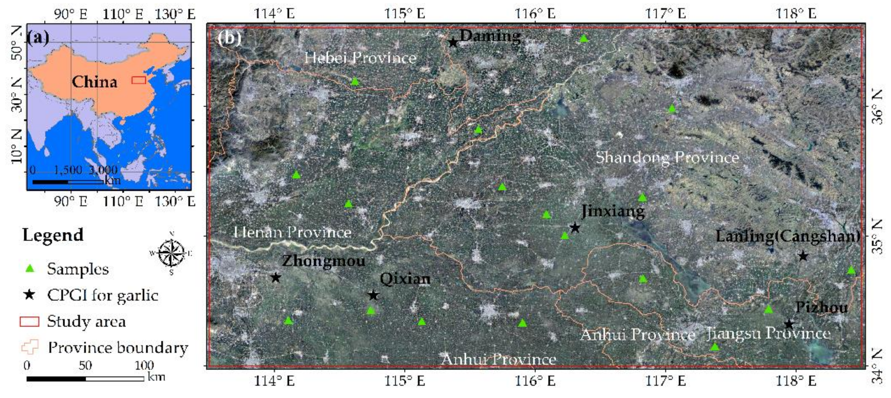
2. Study Area
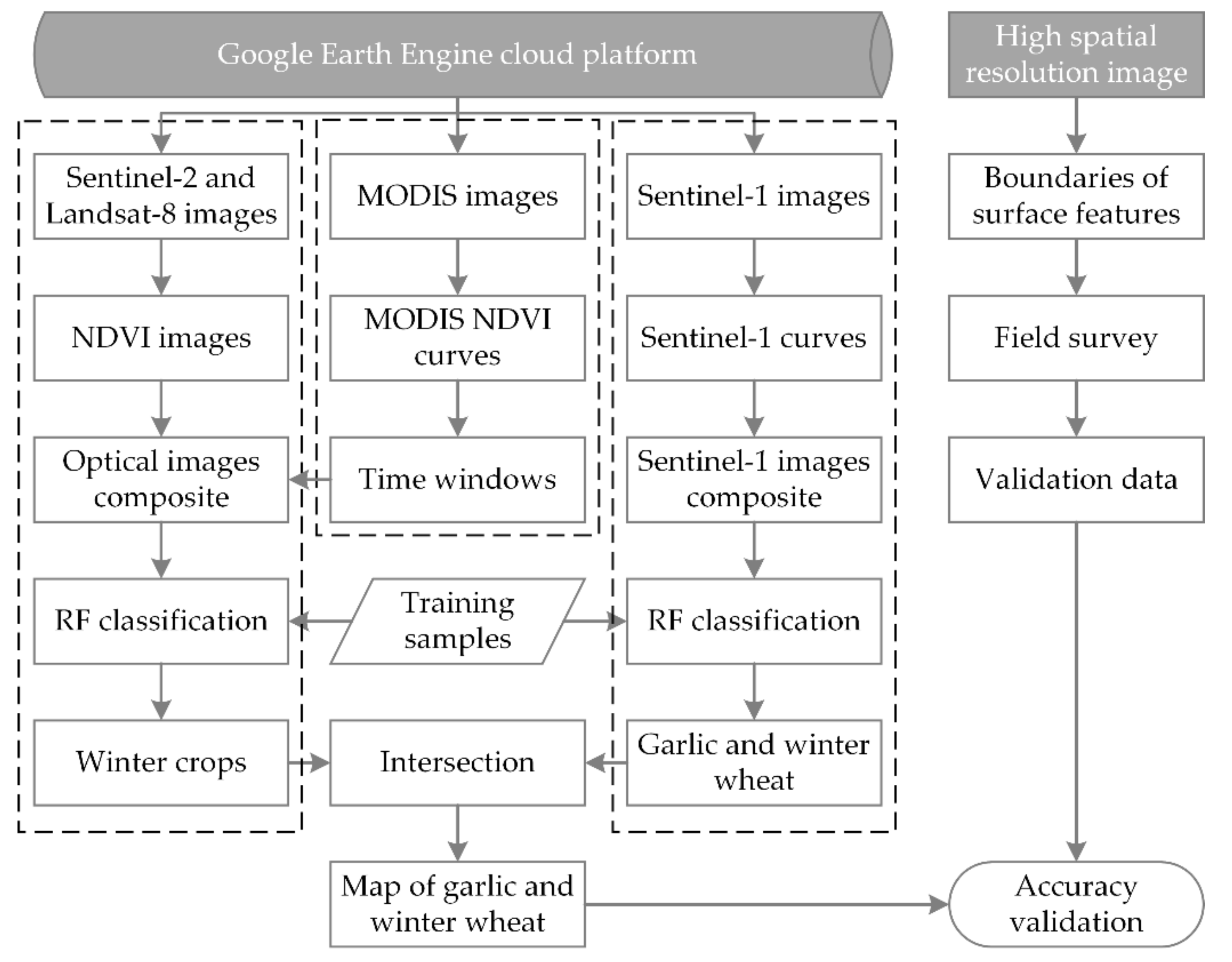
3. Materials and Methods
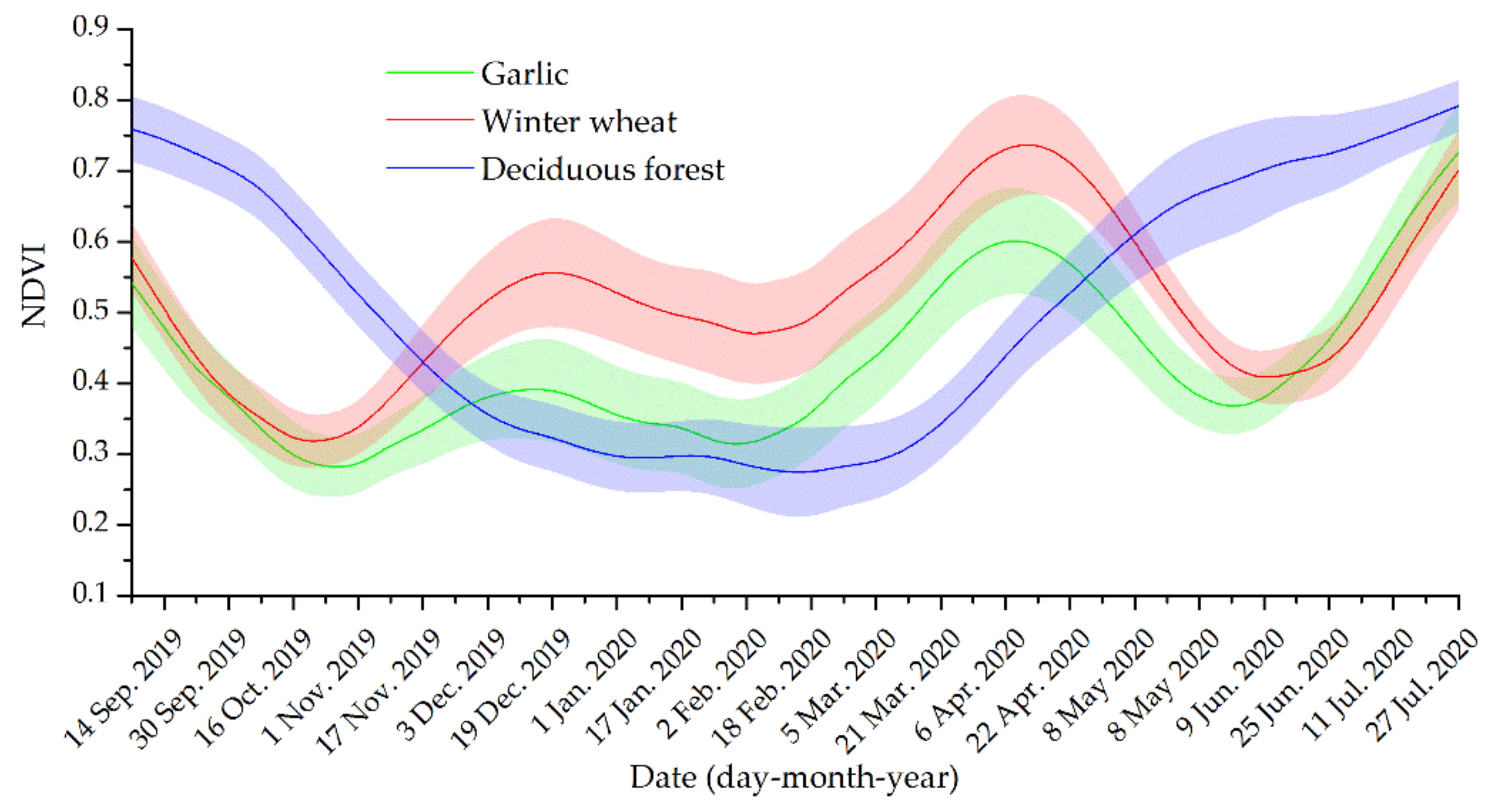
3.1. MODIS NDVI Curves and Composition of Sentinel-2 and Landsat-8 Images
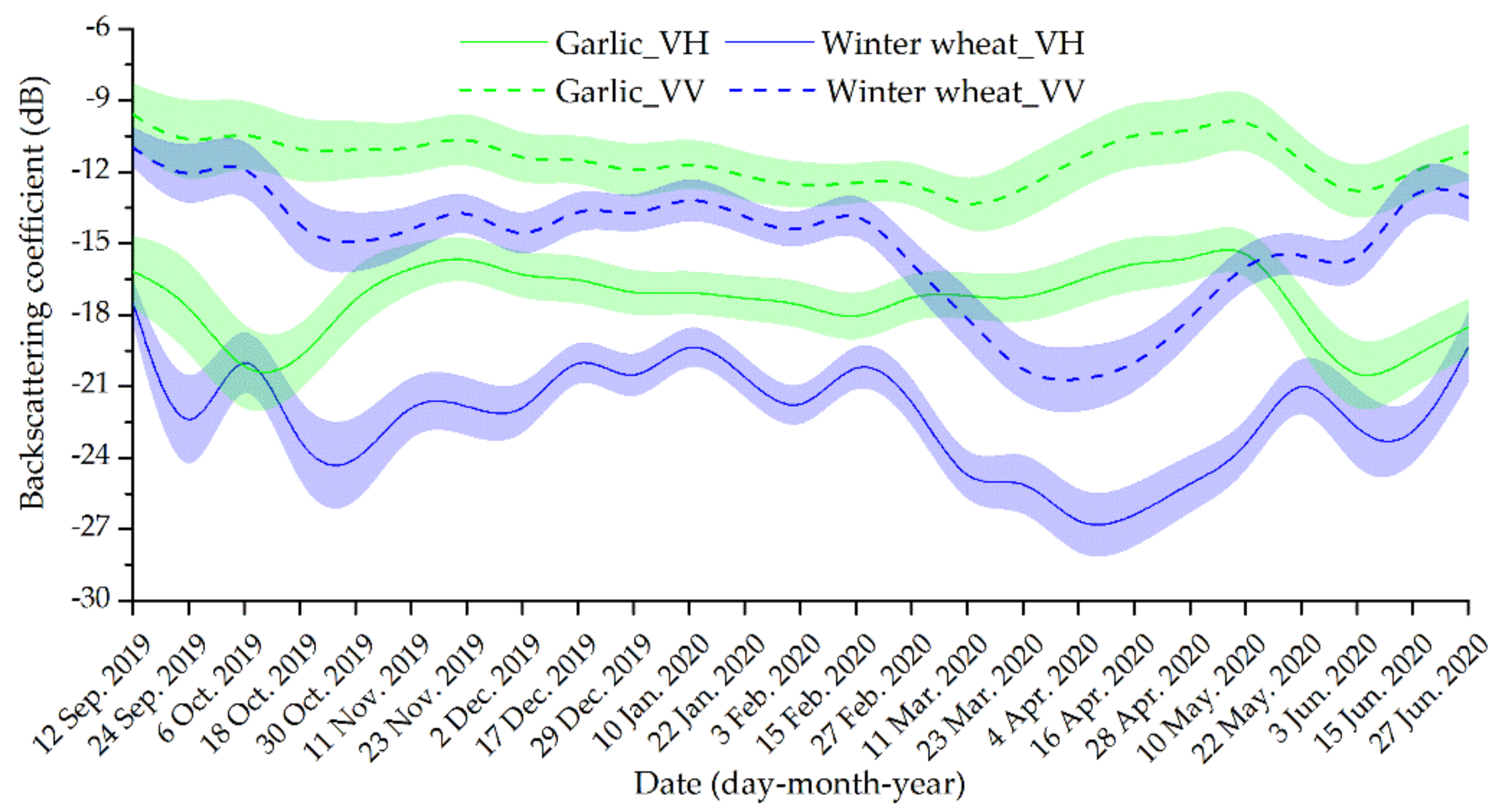
3.2. Sentinel-1 Image Composition
3.3. Garlic and Winter Wheat Identification
3.4. Accuracy Validation
4. Results
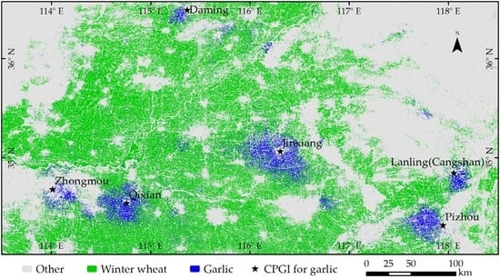
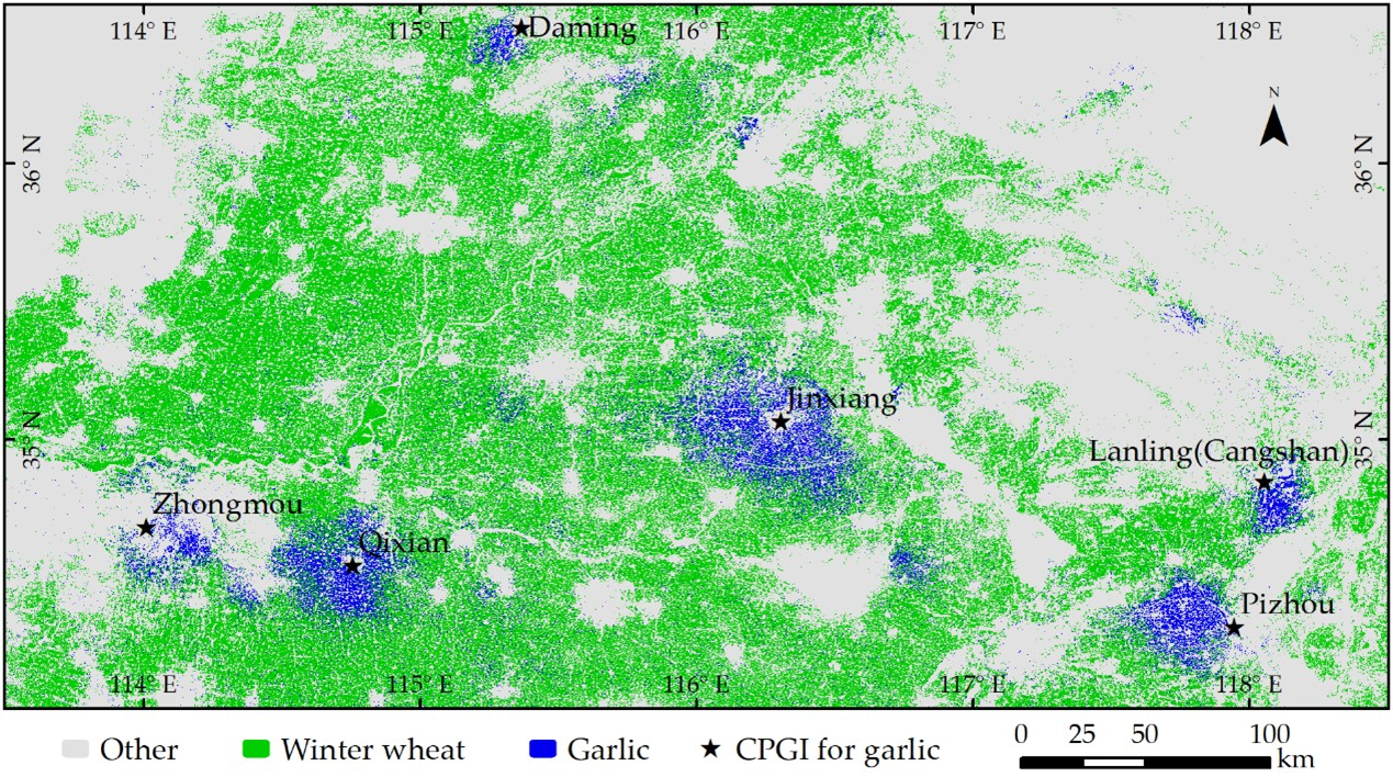
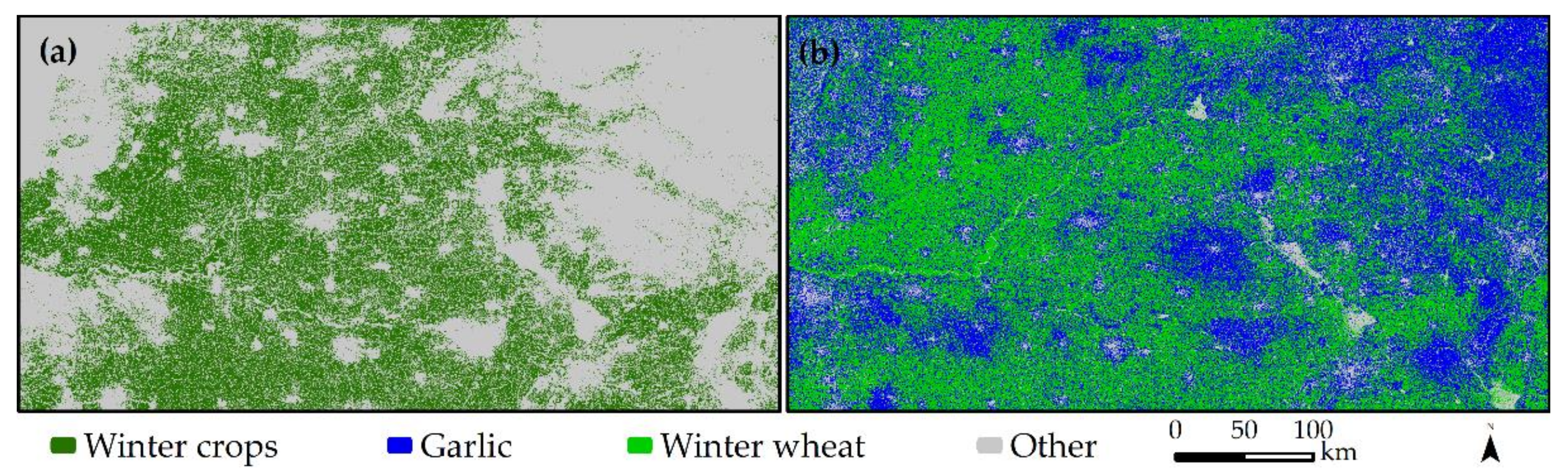
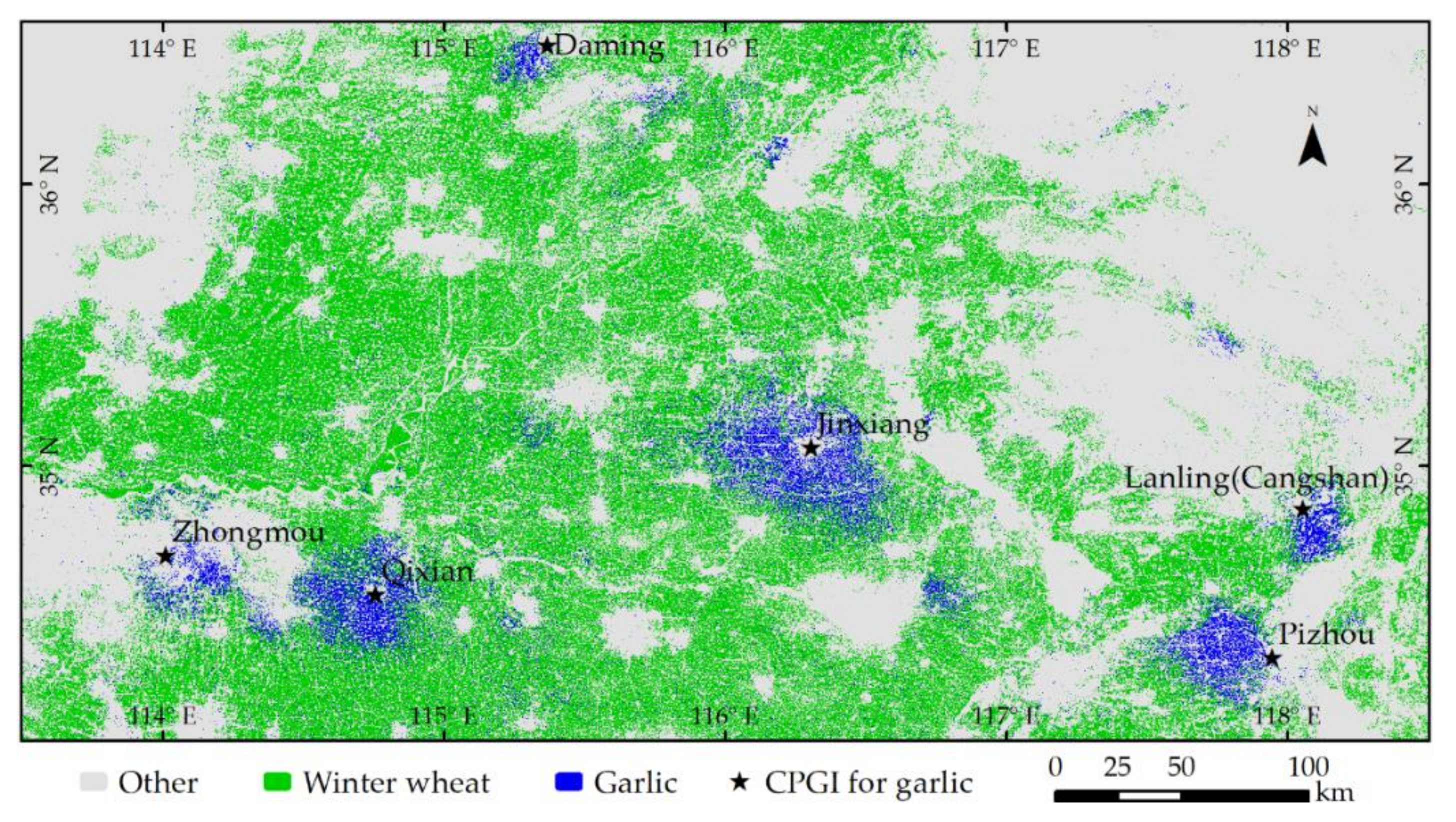
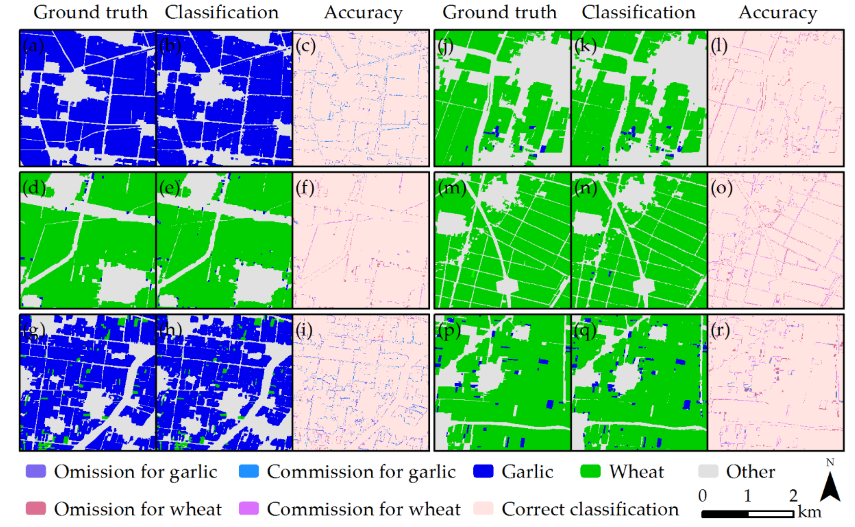
4.1. Classification Results
4.2. Accuracy
5. Discussion
6. Conclusions
Author Contributions
Funding
Conflicts of Interest
Appendix A
- var geometry = ee.Geometry.Rectangle([113.5,33.9,118.5,36.6]);
- var names = ‘optical_’;
- var month_min=[‘2019-10-1’,‘2019-11-1’,‘2020-5-20’,‘2020-7-1’];
- var month_max=[‘2019-12-1’,‘2020-3-20’];
- function maskS2clouds(image) {
- var qa = image.select(‘QA60’);
- var cloudBitMask = 1 << 10;
- var cirrusBitMask = 1 << 11;
- var mask = qa.bitwiseAnd(cloudBitMask).eq(0).and(qa.bitwiseAnd(cirrusBitMask).eq(0));
- return image.updateMask(mask).divide(10000).select(“B.*”).copyProperties(image, [“system:time_start”])}
- var maskL8 = function(image) {
- var qa = image.select(‘BQA’);
- var mask = qa.bitwiseAnd(1 << 4).eq(0);
- return image.updateMask(mask);};
- var kernel = ee.Kernel.square({radius: 1});
- var medianFilter = function(image){return image.addBands(image.focal_median({kernel: kernel, iterations: 1}))};
- var addNDVI = function(image){
- return image.addBands(image.normalizedDifference([‘nir’,’red’]).rename(‘ndvi’));};
- var s2b10 = [‘B2’, ‘B3’, ‘B4’, ‘B8’];
- var lan8 = [‘B2’, ‘B3’, ‘B4’, ‘B5’];
- var STD_NAMES_s2 = [‘blue’,‘green’,‘red’,‘nir’];
- var percentiles =[0,10,20,30,40,50,60,70,80,90,100];
- var sen2_1 = ee.ImageCollection(‘COPERNICUS/S2’)
- .filterDate(month_min[0], month_min[1])
- .filterBounds(geometry)
- .filter(ee.Filter.lt(‘CLOUDY_PIXEL_PERCENTAGE’, 20))
- .map(maskS2clouds)
- .select(s2b10,STD_NAMES_s2);
- var sen2_2 = ee.ImageCollection(‘COPERNICUS/S2’)
- .filterDate(month_min[2], month_min[3])
- .filterBounds(geometry)
- .filter(ee.Filter.lt(‘CLOUDY_PIXEL_PERCENTAGE’, 20))
- .map(maskS2clouds)
- .select(s2b10,STD_NAMES_s2);
- var lan8_1 = ee.ImageCollection(‘LANDSAT/LC08/C01/T1_TOA’)
- .filterDate(month_min[0], month_min[1])
- .filterBounds(geometry)
- .map(maskL8)
- .select(lan8,STD_NAMES_s2);
- var lan8_2 = ee.ImageCollection(‘LANDSAT/LC08/C01/T1_TOA’)
- .filterDate(month_min[2], month_min[3])
- .filterBounds(geometry)
- .map(maskL8)
- .select(lan8,STD_NAMES_s2);
- var lan8_min = ee.ImageCollection(lan8_1.merge(lan8_2));
- var sen2_min = ee.ImageCollection(sen2_1.merge(sen2_2).merge(lan8_min));
- var sen2_ndvi_min = sen2_min.map(addNDVI).select(‘ndvi’).min().clip(geometry);
- var sen2_ndvi_med = sen2_min.map(addNDVI).select(‘ndvi’).median().clip(geometry);
- var sen2_max = ee.ImageCollection(‘COPERNICUS/S2’)
- .filterDate(month_max[0], month_max[1])
- .filterBounds(geometry)
- .filter(ee.Filter.lt(‘CLOUDY_PIXEL_PERCENTAGE’, 20))
- .map(maskS2clouds)
- .select(s2b10,STD_NAMES_s2);
- var sen2_ndvi_max = sen2_max.map(addNDVI).select(‘ndvi’).max().clip(geometry);
- var sen_comp = sen2_ndvi_max.addBands(sen2_ndvi_min).addBands(sen2_ndvi_med);
- Map.addLayer(sen_comp,{min: 0, max: 0.8},‘sen_comp’);
- var features = [winter,other];
- var sample = ee.FeatureCollection(features);
- var training = sen_comp.sampleRegions({collection:sample, properties: [‘class’], scale: 10});
- var rf_classifier = ee.Classifier.randomForest(100).train(training, ‘class’);
- var RF_classified = sen_comp.classify(rf_classifier);
- var RF_classified = ee.Image(RF_classified).int8();
- Map.addLayer(RF_classified,{min: 0, max:2},‘RF_classified’);
- Export.image.toDrive({
- image:RF_classified,
- description:names+‘ndvi_class’,
- fileNamePrefix: names+‘ndvi_class’,
- scale: 10,
- region: geometry,
- maxPixels: 900000000000});
Appendix B
- var geometry = ee.Geometry.Rectangle([113.5,33.9,118.5,37]);var names = ‘s1_’;
- var month1=[‘2020-1-1’,‘2020-2-16’];
- var month2=[‘2020-4-1’,‘2020-5-1’];
- var month3=[‘2020-6-1’,‘2020-6-16’];
- var nodataMask1 = function(img) { var score1 =img.select(‘VH’); return img.updateMask(score1.gt(-30)); };
- var nodataMask2 = function(img) { var score2 =img.select(‘VV’); return img.updateMask(score2.gt(-28)); };
- var kernel = ee.Kernel.square({radius: 1});
- var medianFilter = function(image){ return image.addBands(image.focal_median({kernel: kernel, iterations: 1}))};
- var s1_1 = ee.ImageCollection(‘COPERNICUS/S1_GRD’)
- .filterBounds(geometry)
- .filterDate(month1[0], month1[1])
- .filter(ee.Filter.listContains(‘transmitterReceiverPolarisation’, ‘VH’))
- .filter(ee.Filter.listContains(‘transmitterReceiverPolarisation’, ‘VV’))
- .map(nodataMask1)
- .map(nodataMask2)
- .map(medianFilter);
- var s1_1_vh = s1_1.select(‘VH’).median();
- var s1_1_vv = s1_1.select(‘VV’).median();
- var s1_2 = ee.ImageCollection(‘COPERNICUS/S1_GRD’)
- .filterBounds(geometry)
- .filterDate(month2[0], month2[1])
- .filter(ee.Filter.listContains(‘transmitterReceiverPolarisation’, ‘VH’))
- .filter(ee.Filter.listContains(‘transmitterReceiverPolarisation’, ‘VV’))
- .map(nodataMask1)
- .map(nodataMask2)
- .map(medianFilter);
- var s1_2_vh = s1_2.select(‘VH’).median();
- var s1_2_vv = s1_2.select(‘VV’).median();
- var s1_3 = ee.ImageCollection(‘COPERNICUS/S1_GRD’)
- .filterBounds(geometry)
- .filterDate(month3[0], month3[1])
- .filter(ee.Filter.listContains(‘transmitterReceiverPolarisation’, ‘VH’))
- .filter(ee.Filter.listContains(‘transmitterReceiverPolarisation’, ‘VV’))
- .map(nodataMask1)
- .map(nodataMask2)
- .map(medianFilter);
- var s1_3_vh = s1_3.select(‘VH’).median();
- var s1_3_vv = s1_3.select(‘VV’).median();
- var s1_img = s1_1_vv.addBands(s1_2_vv).addBands(s1_1_vh).addBands(s1_2_vh).addBands(s1_3_vh);
- Map.addLayer(s1_img,{min: -30, max: 0},‘s1_img’);
- Map.centerObject(s1_img, 7);
- var features = [garlic,wheat,other]
- var sample = ee.FeatureCollection(features)
- var training = s1_img.sampleRegions({ collection:sample, properties: [‘class’], scale: 10});
- var rf_classifier = ee.Classifier.randomForest(100).train(training, ‘class’);
- var RF_classified = s1_img.classify(rf_classifier);
- var RF_classified = ee.Image(RF_classified).int8();
- Map.addLayer(RF_classified,{min: 1, max:3},‘RF_classified’);
- Export.image.toDrive({
- image:RF_classified,
- description:names+‘sar_class’,
- fileNamePrefix:names+‘sar_class’,
- scale: 10,
- region: geometry,
- maxPixels: 900000000000});
References
- Xie, Y.; Wang, P.X.; Bai, X.J.; Khan, J.; Zhang, S.Y.; Li, L.; Wang, L. Assimilation of the leaf area index and vegetation temperature condition index for winter wheat yield estimation using landsat imagery and the ceres-wheat model. Agric. Forest Meteorol. 2017, 246, 194–206. [Google Scholar] [CrossRef]
- Qiu, B.W.; Luo, Y.H.; Tang, Z.H.; Chen, C.C.; Lu, D.F.; Huang, H.Y.; Chen, Y.Z.; Chen, N.; Xu, W.M. Winter wheat mapping combining variations before and after estimated heading dates. ISPRS J. Photogramm. Remote Sens. 2017, 123, 35–46. [Google Scholar] [CrossRef]
- Huang, J.; Tian, L.; Liang, S.; Ma, H.; Becker-Reshef, I.; Huang, Y.; Su, W.; Zhang, X.; Zhu, D.; Wu, W. Improving winter wheat yield estimation by assimilation of the leaf area index from landsat tm and modis data into the wofost model. Agric. Forest Meteorol. 2015, 204, 106–121. [Google Scholar] [CrossRef] [Green Version]
- Tian, H.F.; Huang, N.; Niu, Z.; Qin, Y.C.; Pei, J.; Wang, J. Mapping Winter Crops in China with Multi-Source Satellite Imagery and Phenology-Based Algorithm. Remote Sens. 2019, 11, 820. [Google Scholar] [CrossRef] [Green Version]
- Ma, Y.P.; Wang, S.L.; Zhang, L.; Hou, Y.Y.; Zhuang, L.W.; He, Y.B.; Wang, F.T. Monitoring winter wheat growth in North China by combining a crop model and remote sensing data. Int. J. Appl. Earth Obs. Geoinf. 2008, 10, 426–437. [Google Scholar] [CrossRef]
- Dominguez, J.A.; Kumhalova, J.; Novak, P. Winter oilseed rape and winter wheat growth prediction using remote sensing methods. Plant Soil Environ. 2015, 61, 410–416. [Google Scholar] [CrossRef] [Green Version]
- Yang, N.; Liu, D.; Feng, Q.; Xiong, Q.; Zhang, L.; Ren, T.; Zhao, Y.; Zhu, D.; Huang, J. Large-Scale Crop Mapping Based on Machine Learning and Parallel Computation with Grids. Remote Sens. 2019, 11, 1500. [Google Scholar] [CrossRef] [Green Version]
- Franke, J.; Menz, G. Multi-temporal wheat disease detection by multi-spectral remote sensing. Precis. Agric. 2007, 8, 161–172. [Google Scholar] [CrossRef]
- Tian, H.F.; Wu, M.Q.; Wang, L.; Niu, Z. Mapping Early, Middle and Late Rice Extent Using Sentinel-1A and Landsat-8 Data in the Poyang Lake Plain, China. Sensors 2018, 18, 185. [Google Scholar] [CrossRef] [Green Version]
- Wang, J.; Wu, C.; Wang, X.; Zhang, X. A new algorithm for the estimation of leaf unfolding date using MODIS data over China’s terrestrial ecosystems. ISPRS J. Photogramm. Remote Sens. 2019, 149, 77–90. [Google Scholar] [CrossRef]
- Tao, J.B.; Wu, W.B.; Zhou, Y.; Wang, Y.; Jiang, Y. Mapping winter wheat using phenological feature of peak before winter on the North China Plain based on time-series MODIS data. J. Integr. Agric. 2017, 16, 348–359. [Google Scholar] [CrossRef]
- Sun, H.S.; Xu, A.G.; Lin, H.; Zhang, L.P.; Mei, Y. Winter wheat mapping using temporal signatures of MODIS vegetation index data. Int. J. Remote Sens. 2012, 33, 5026–5042. [Google Scholar] [CrossRef]
- Pan, Y.Z.; Li, L.; Zhang, J.S.; Liang, S.L.; Zhu, X.F.; Sulla-Menashe, D. Winter wheat area estimation from MODIS-EVI time series data using the Crop Proportion Phenology Index. Remote Sens. Environ. 2012, 119, 232–242. [Google Scholar] [CrossRef]
- Pasqualotto, N.; Delegido, J.; Van Wittenberghe, S.; Rinaldi, M.; Moreno, J. Multi-Crop Green LAI Estimation with a New Simple Sentinel-2 LAI Index (SeLI). Sensors 2019, 19, 904. [Google Scholar] [CrossRef] [PubMed] [Green Version]
- Zhu, J.; Pan, Z.W.; Wang, H.; Huang, P.J.; Sun, J.L.; Qin, F.; Liu, Z.Z. An Improved Multi-temporal and Multi-feature Tea Plantation Identification Method Using Sentinel-2 Imagery. Sensors 2019, 19, 2087. [Google Scholar] [CrossRef] [Green Version]
- Ahmadian, N.; Ghasemi, S.; Wigneron, J.P.; Zolitz, R. Comprehensive study of the biophysical parameters of agricultural crops based on assessing Landsat 8 OLI and Landsat 7 ETM+ vegetation indices. Gisci. Remote Sens. 2016, 53, 337–359. [Google Scholar] [CrossRef]
- Ozelkan, E.; Chen, G.; Ustundag, B.B. Multiscale object-based drought monitoring and comparison in rainfed and irrigated agriculture from Landsat 8 OLI imagery. Int. J. Appl. Earth Obs. Geoinf. 2016, 44, 159–170. [Google Scholar] [CrossRef]
- Xiong, J.; Thenkabail, P.S.; Gumma, M.K.; Teluguntla, P.; Poehnelt, J.; Congalton, R.G.; Yadav, K.; Thau, D. Automated cropland mapping of continental Africa using Google Earth Engine cloud computing. ISPRS J. Photogramm. Remote Sens. 2017, 126, 225–244. [Google Scholar] [CrossRef] [Green Version]
- Chen, F.; Zhang, M.M.; Tian, B.S.; Li, Z. Extraction of Glacial Lake Outlines in Tibet Plateau Using Landsat 8 Imagery and Google Earth Engine. IEEE J. Sel. Top. Appl. Earth Obs. Remote Sens. 2017, 10, 4002–4009. [Google Scholar] [CrossRef]
- Teluguntla, P.; Thenkabail, P.S.; Oliphant, A.; Xiong, J.; Gumma, M.K.; Congalton, R.G.; Yadav, K.; Huete, A. A 30-m landsat-derived cropland extent product of Australia and China using random forest machine learning algorithm on Google Earth Engine cloud computing platform. ISPRS J. Photogramm. Remote Sens. 2018, 144, 325–340. [Google Scholar] [CrossRef]
- Gorelick, N.; Hancher, M.; Dixon, M.; Ilyushchenko, S.; Thau, D.; Moore, R. Google Earth Engine: Planetary-scale geospatial analysis for everyone. Remote Sens. Environ. 2017, 202, 18–27. [Google Scholar] [CrossRef]
- Traganos, D.; Aggarwal, B.; Poursanidis, D.; Topouzelis, K.; Chrysoulakis, N.; Reinartz, P. Towards Global-Scale Seagrass Mapping and Monitoring Using Sentinel-2 on Google Earth Engine: The Case Study of the Aegean and Ionian Seas. Remote Sens. 2018, 10, 1227. [Google Scholar] [CrossRef] [Green Version]
- Tsai, Y.H.; Stow, D.; Chen, H.L.; Lewison, R.; An, L.; Shi, L. Mapping Vegetation and Land Use Types in Fanjingshan National Nature Reserve Using Google Earth Engine. Remote Sens. 2018, 10, 927. [Google Scholar] [CrossRef] [Green Version]
- Pei, J.; Wang, L.; Wang, X.; Niu, Z.; Cao, J. Time Series of Landsat Imagery Shows Vegetation Recovery in Two Fragile Karst Watersheds in Southwest China from 1988 to 2016. Remote Sens. 2019, 11, 2044. [Google Scholar] [CrossRef] [Green Version]
- Jin, Z.N.; Azzari, G.; You, C.; Di Tommaso, S.; Aston, S.; Burke, M.; Lobell, D.B. Smallholder maize area and yield mapping at national scales with Google Earth Engine. Remote Sens. Environ. 2019, 228, 115–128. [Google Scholar] [CrossRef]
- Hansen, M.C.; Potapov, P.V.; Moore, R.; Hancher, M.; Turubanova, S.A.; Tyukavina, A.; Thau, D.; Stehman, S.V.; Goetz, S.J.; Loveland, T.R.; et al. High-Resolution Global Maps of 21st-Century Forest Cover Change. Science 2013, 342, 850–853. [Google Scholar] [CrossRef] [Green Version]
- Sakamoto, T.; Yokozawa, M.; Toritani, H.; Shibayama, M.; Ishitsuka, N.; Ohno, H. A crop phenology detection method using time-series MODIS data. Remote Sens. Environ. 2005, 96, 366–374. [Google Scholar] [CrossRef]
- Cai, Y.P.; Guan, K.Y.; Peng, J.; Wang, S.W.; Seifert, C.; Wardlow, B.; Li, Z. A high-performance and in-season classification system of field-level crop types using time-series Landsat data and a machine learning approach. Remote Sens. Environ. 2018, 210, 35–47. [Google Scholar] [CrossRef]
- Sakamoto, T.; Wardlow, B.D.; Gitelson, A.A.; Verma, S.B.; Suyker, A.E.; Arkebauer, T.J. A Two-Step Filtering approach for detecting maize and soybean phenology with time-series MODIS data. Remote Sens. Environ. 2010, 114, 2146–2159. [Google Scholar] [CrossRef]
- Wang, J.; Wu, C.; Zhang, C.; Ju, W.; Wang, X.; Chen, Z.; Fang, B. Improved modeling of gross primary productivity (GPP) by better representation of plant phenological indicators from remote sensing using a process model. Ecol. Indic. 2018, 88, 332–340. [Google Scholar] [CrossRef]
- Tian, H.F.; Li, W.; Wu, M.Q.; Huang, N.; Li, G.D.; Li, X.; Niu, Z. Dynamic Monitoring of the Largest Freshwater Lake in China Using a New Water Index Derived from High Spatiotemporal Resolution Sentinel-1A Data. Remote Sens. 2017, 9, 521. [Google Scholar] [CrossRef] [Green Version]
- Zhu, Z.; Woodcock, C.E. Object-based cloud and cloud shadow detection in Landsat imagery. Remote Sens. Environ. 2012, 118, 83–94. [Google Scholar] [CrossRef]
- Mandal, D.; Kumar, V.; Ratha, D.; Dey, S.; Bhattacharya, A.; Lopez-Sanchez, J.M.; McNairn, H.; Rao, Y.S. Dual polarimetric radar vegetation index for crop growth monitoring using sentinel-1 SAR data. Remote Sens. Environ. 2020, 247, 111954. [Google Scholar] [CrossRef]
- Fikriyah, V.N.; Darvishzadeh, R.; Laborte, A.; Khan, N.I.; Nelson, A. Discriminating transplanted and direct seeded rice using Sentinel-1 intensity data. Int. J. Appl. Earth Obs. Geoinf. 2019, 76, 143–153. [Google Scholar] [CrossRef] [Green Version]
- Singha, M.; Dong, J.W.; Zhang, G.L.; Xiao, X.M. High resolution paddy rice maps in cloud-prone Bangladesh and Northeast India using Sentinel-1 data. Sci. Data 2019, 6, 26. [Google Scholar] [CrossRef] [PubMed]
- d’Andrimont, R.; Taymans, M.; Lemoine, G.; Ceglar, A.; Yordanov, M.; van der Velde, M. Detecting flowering phenology in oil seed rape parcels with Sentinel-1 and-2 time series. Remote Sens. Environ. 2020, 239, 111660. [Google Scholar] [CrossRef] [PubMed]
- Chauhan, S.; Darvishzadeh, R.; Lu, Y.; Boschetti, M.; Nelson, A. Understanding wheat lodging using multi-temporal Sentinel-1 and Sentinel-2 data. Remote Sens. Environ. 2020, 243. [Google Scholar] [CrossRef]
- Cable, J.W.; Kovacs, J.M.; Jiao, X.F.; Shang, J.L. Agricultural Monitoring in Northeastern Ontario, Canada, Using Multi-Temporal Polarimetric RADARSAT-2 Data. Remote Sens. 2014, 6, 2343–2371. [Google Scholar] [CrossRef] [Green Version]
- Luo, Y.M.; Huang, D.T.; Liu, P.Z.; Feng, H.M. An novel random forests and its application to the classification of mangroves remote sensing image. Multimed. Tools Appl. 2016, 75, 9707–9722. [Google Scholar] [CrossRef]
- Yu, Y.; Li, M.Z.; Fu, Y. Forest type identification by random forest classification combined with SPOT and multitemporal SAR data. J. For. Res. 2018, 29, 1407–1414. [Google Scholar] [CrossRef]
- Abdullah, A.Y.M.; Masrur, A.; Adnan, M.S.G.; Al Baky, M.A.; Hassan, Q.K.; Dewan, A. Spatio-Temporal Patterns of Land Use/Land Cover Change in the Heterogeneous Coastal Region of Bangladesh between 1990 and 2017. Remote Sens. 2019, 11, 790. [Google Scholar] [CrossRef] [Green Version]
- Bangira, T.; Alfieri, S.M.; Menenti, M.; van Niekerk, A. Comparing Thresholding with Machine Learning Classifiers for Mapping Complex Water. Remote Sens. 2019, 11, 1351. [Google Scholar] [CrossRef] [Green Version]
- Mountrakis, G.; Im, J.; Ogole, C. Support vector machines in remote sensing: A review. ISPRS J. Photogramm. Remote Sens. 2011, 66, 247–259. [Google Scholar] [CrossRef]
- Reichstein, M.; Camps-Valls, G.; Stevens, B.; Jung, M.; Denzler, J.; Carvalhais, N.; Prabhat. Deep learning and process understanding for data-driven Earth system science. Nature 2019, 566, 195–204. [Google Scholar] [CrossRef] [PubMed]
- Wang, X.; Huang, J.; Feng, Q.; Yin, D. Winter Wheat Yield Prediction at County Level and Uncertainty Analysis in Main Wheat-Producing Regions of China with Deep Learning Approaches. Remote Sens. 2020, 12, 1744. [Google Scholar] [CrossRef]
- Sun, D.L.; Yu, Y.Y.; Goldberg, M.D. Deriving Water Fraction and Flood Maps From MODIS Images Using a Decision Tree Approach. IEEE J. Sel. Top. Appl. Earth Obs. Remote Sens. 2011, 4, 814–825. [Google Scholar] [CrossRef]
- Xu, M.; Watanachaturaporn, P.; Varshney, P.K.; Arora, M.K. Decision tree regression for soft classification of remote sensing data. Remote Sens. Environ. 2005, 97, 322–336. [Google Scholar] [CrossRef]
- Li, L.Y.; Chen, Y.; Xu, T.B.; Shi, K.F.; Liu, R.; Huang, C.; Lu, B.B.; Meng, L.K. Remote Sensing of Wetland Flooding at a Sub-Pixel Scale Based on Random Forests and Spatial Attraction Models. Remote Sens. 2019, 11, 1231. [Google Scholar] [CrossRef] [Green Version]
- Amani, M.; Salehi, B.; Mahdavi, S.; Granger, J.; Brisco, B. Wetland classification in Newfoundland and Labrador using multi-source SAR and optical data integration. Gisci. Remote Sens. 2017, 54, 779–796. [Google Scholar] [CrossRef]
- Houborg, R.; McCabe, M.F. A hybrid training approach for leaf area index estimation via Cubist and random forests machine-learning. ISPRS J. Photogramm. Remote Sens. 2018, 135, 173–188. [Google Scholar] [CrossRef]
- Breiman, L. Random forests. Mach. Learn. 2001, 45, 5–32. [Google Scholar] [CrossRef] [Green Version]
- Rodriguez-Galiano, V.F.; Ghimire, B.; Rogan, J.; Chica-Olmo, M.; Rigol-Sanchez, J.P. An assessment of the effectiveness of a random forest classifier for land-cover classification. ISPRS J. Photogramm. Remote Sens. 2012, 67, 93–104. [Google Scholar] [CrossRef]
- Huete, A.; Didan, K.; Miura, T.; Rodriguez, E.P.; Gao, X.; Ferreira, L.G. Overview of the radiometric and biophysical performance of the MODIS vegetation indices. Remote Sens. Environ. 2002, 83, 195–213. [Google Scholar] [CrossRef]
- Lunetta, R.S.; Knight, J.F.; Ediriwickrema, J.; Lyon, J.G.; Worthy, L.D. Land-cover change detection using multi-temporal MODIS NDVI data. Remote Sens. Environ. 2006, 105, 142–154. [Google Scholar] [CrossRef]
- Chen, J.; Jonsson, P.; Tamura, M.; Gu, Z.H.; Matsushita, B.; Eklundh, L. A simple method for reconstructing a high-quality NDVI time-series data set based on the Savitzky-Golay filter. Remote Sens. Environ. 2004, 91, 332–344. [Google Scholar] [CrossRef]
- Card, D.H. Using known map category marginal frequencies to improve estimates of thematic map accuracy. Photogramm. Eng. Remote Sens. 1982, 48, 431–439. [Google Scholar]
- Olofsson, P.; Foody, G.M.; Stehman, S.V.; Woodcock, C.E. Making better use of accuracy data in land change studies: Estimating accuracy and area and quantifying uncertainty using stratified estimation. Remote Sens. Environ. 2013, 129, 122–131. [Google Scholar] [CrossRef]
- Guo, Y.Q.; Jia, X.P.; Paull, D.; Benediktsson, J.A. Nomination-favoured opinion pool for optical-SAR-synergistic rice mapping in face of weakened flooding signals. ISPRS J. Photogramm. Remote Sens. 2019, 155, 187–205. [Google Scholar] [CrossRef]
- Cai, Y.T.; Li, X.Y.; Zhang, M.; Lin, H. Mapping wetland using the object-based stacked generalization method based on multi-temporal optical and SAR data. Int. J. Appl. Earth Obs. Geoinf. 2020, 92, 102164. [Google Scholar] [CrossRef]
- Fretwell, P.T.; Convey, P.; Fleming, A.H.; Peat, H.J.; Hughes, K.A. Detecting and mapping vegetation distribution on the Antarctic Peninsula from remote sensing data. Polar Biol. 2011, 34, 273–281. [Google Scholar] [CrossRef]
- Hmimina, G.; Dufrene, E.; Pontailler, J.Y.; Delpierre, N.; Aubinet, M.; Caquet, B.; de Grandcourt, A.; Burban, B.; Flechard, C.; Granier, A.; et al. Evaluation of the potential of MODIS satellite data to predict vegetation phenology in different biomes: An investigation using ground-based NDVI measurements. Remote Sens. Environ. 2013, 132, 145–158. [Google Scholar] [CrossRef]
- Pastor-Guzman, J.; Dash, J.; Atkinson, P.M. Remote sensing of mangrove forest phenology and its environmental drivers. Remote Sens. Environ. 2018, 205, 71–84. [Google Scholar] [CrossRef] [Green Version]
- Shuai, G.; Zhang, J.; Basso, B.; Pan, Y.; Zhu, X.; Zhu, S.; Liu, H. Multi-temporal RADARSAT-2 polarimetric SAR for maize mapping supported by segmentations from high-resolution optical image. Int. J. Appl. Earth Obs. Geoinf. 2019, 74, 1–15. [Google Scholar] [CrossRef]
- Ju, J.C.; Roy, D.P. The availability of cloud-free Landsat ETM plus data over the conterminous United States and globally. Remote Sens. Environ. 2008, 112, 1196–1211. [Google Scholar] [CrossRef]
- Song, Y.; Wang, J. Mapping Winter Wheat Planting Area and Monitoring Its Phenology Using Sentinel-1 Backscatter Time Series. Remote Sens. 2019, 11, 449. [Google Scholar] [CrossRef] [Green Version]
- Schlund, M.; Erasmi, S. Sentinel-1 time series data for monitoring the phenology of winter wheat. Remote Sens. Environ. 2020, 246. [Google Scholar] [CrossRef]
- Veloso, A.; Mermoz, S.; Bouvet, A.; Toan, T.L.; Planells, M.; Dejoux, J.F.; Ceschia, E. Understanding the temporal behavior of crops using Sentinel-1 and Sentinel-2-like data for agricultural applications. Remote Sens. Environ. 2017, 199, 415–426. [Google Scholar] [CrossRef]
- Jia, M.Q.; Tong, L.; Zhang, Y.Z.; Chen, Y. Multitemporal radar backscattering measurement of wheat fields using multifrequency (L, S, C, and X) and full-polarization. Radio Sci. 2013, 48, 471–481. [Google Scholar] [CrossRef]
- Zhang, H.S.; Xu, R. Exploring the optimal integration levels between SAR and optical data for better urban land cover mapping in the Pearl River Delta. Int. J. Appl. Earth Obs. Geoinf. 2018, 64, 87–95. [Google Scholar] [CrossRef]
- Steinhausen, M.J.; Wagner, P.D.; Narasimhan, B.; Waske, B. Combining Sentinel-1 and Sentinel-2 data for improved land use and land cover mapping of monsoon regions. Int. J. Appl. Earth Obs. Geoinf. 2018, 73, 595–604. [Google Scholar] [CrossRef]


| Class Results | Ground Truth (Pixels) | User’s Accuracy | Producer’s Accuracy | |
|---|---|---|---|---|
| Winter Crops | Other | |||
| Winter crops | 1,134,648 | 40,614 | 96.54% | 97.99% |
| Other | 23,244 | 432,312 | 94.90% | 91.41% |
| Class Results | Ground Truth (pixels) | User’s Accuracy | Producer’s Accuracy | ||
|---|---|---|---|---|---|
| Garlic | Winter Wheat | Other | |||
| Garlic | 379,029 | 24,531 | 294,453 | 54.30% | 98.42% |
| Winter wheat | 4335 | 747,354 | 104,301 | 87.31% | 96.71% |
| Other | 1761 | 882 | 74,172 | 96.56% | 15.68% |
| Class Results | Ground Truth (pixels) | User’s Accuracy | Producer’s Accuracy | ||
|---|---|---|---|---|---|
| Garlic | Winter Wheat | Other | |||
| Garlic | 369,138 | 5493 | 10,551 | 95.83% | 95.85% |
| Winter wheat | 2295 | 753,054 | 19,425 | 97.20% | 97.45% |
| Other | 13,692 | 14,220 | 442,950 | 94.72% | 93.66% |
Publisher’s Note: MDPI stays neutral with regard to jurisdictional claims in published maps and institutional affiliations. |
© 2020 by the authors. Licensee MDPI, Basel, Switzerland. This article is an open access article distributed under the terms and conditions of the Creative Commons Attribution (CC BY) license (http://creativecommons.org/licenses/by/4.0/).
Share and Cite
Tian, H.; Pei, J.; Huang, J.; Li, X.; Wang, J.; Zhou, B.; Qin, Y.; Wang, L. Garlic and Winter Wheat Identification Based on Active and Passive Satellite Imagery and the Google Earth Engine in Northern China. Remote Sens. 2020, 12, 3539. https://0-doi-org.brum.beds.ac.uk/10.3390/rs12213539
Tian H, Pei J, Huang J, Li X, Wang J, Zhou B, Qin Y, Wang L. Garlic and Winter Wheat Identification Based on Active and Passive Satellite Imagery and the Google Earth Engine in Northern China. Remote Sensing. 2020; 12(21):3539. https://0-doi-org.brum.beds.ac.uk/10.3390/rs12213539
Chicago/Turabian StyleTian, Haifeng, Jie Pei, Jianxi Huang, Xuecao Li, Jian Wang, Boyan Zhou, Yaochen Qin, and Li Wang. 2020. "Garlic and Winter Wheat Identification Based on Active and Passive Satellite Imagery and the Google Earth Engine in Northern China" Remote Sensing 12, no. 21: 3539. https://0-doi-org.brum.beds.ac.uk/10.3390/rs12213539