A Modified Geometrical Optical Model of Row Crops Considering Multiple Scattering Frame


College of Earth and Environmental Sciences, Lanzhou University, Lanzhou 730000, China
*
Author to whom correspondence should be addressed.
Remote Sens. 2020, 12(21), 3600; https://0-doi-org.brum.beds.ac.uk/10.3390/rs12213600
Submission received: 21 September 2020
/
Revised: 16 October 2020
/
Accepted: 27 October 2020
/
Published: 2 November 2020
(This article belongs to the Special Issue Crop Disease Detection Using Remote Sensing Image Analysis)
Abstract
:The canopy reflectance model is the physical basis of remote sensing inversion. In canopy reflectance modeling, the geometric optical (GO) approach is the most commonly used. However, it ignores the description of a multiple-scattering contribution, which causes an underestimation of the reflectance. Although researchers have tried to add a multiple-scattering contribution to the GO approach for forest modeling, different from forests, row crops have unique geometric characteristics. Therefore, the modeling approach originally applied to forests cannot be directly applied to row crops. In this study, we introduced the adding method and mathematical solution of integral radiative transfer equation into row modeling, and on the basis of improving the overlapping relationship of the gap probabilities involved in the single-scattering contribution, we derived multiple-scattering equations suitable for the GO approach. Based on these modifications, we established a row model that can accurately describe the single-scattering and multiple-scattering contributions in row crops. We validated the row model using computer simulations and in situ measurements and found that it can be used to simulate crop canopy reflectance at different growth stages. Moreover, the row model can be successfully used to simulate the distribution of reflectances (RMSEs < 0.0404). During computer validation, the row model also maintained high accuracy (RMSEs < 0.0062). Our results demonstrate that considering multiple scattering in GO-approach-based modeling can successfully address the underestimation of reflectance in the row crops.

1. Introduction
In recent canopy modeling studies, row modeling has been extensively studied. The canopy modeling of crops based on the row model can more accurately estimate the seasonal changes of biophysical canopy parameters in remote sensing [1]. In the inversion of remote sensing, physical modeling is key, and its approach can be separated into three categories based on different physical mechanisms, name the computer simulation (CS) approach, radiative transfer (RT) approach, and geometric optical (GO) approach [2]. The GO approach can describe the geometric characteristics of an individual canopy. It is most suitable for heterogeneous canopy modeling [3]. The CS approach has the highest accuracy and has been applied primarily for understanding radiation regimes. It has been used as a “truth value” (“surrogate truth” or benchmark in Radiation Transfer Model Intercomparison (RAMI)) [4,5,6] to validate GO and RT approaches. However, compared to the GO approach, the computational time of the CS approach is too slow; hence, it is rarely used in remote sensing inversion. The RT approach is based on volume scattering in the radiative transfer equation. It is very suitable for describing the scattering issue in canopies [7]. However, compared to the GO approach, the RT approach lacks a description of the geometric characteristics of an individual canopy and is mostly used for high-density homogeneous (or continuous) canopy modeling [2]. The row crop is a heterogeneous canopy. It has the typical geometric characteristics of an individual canopy, such as row structure (e.g., height, row width, between-row distance, etc.) [8,9,10,11]. Therefore, considering the advantages of accurately describing the row structure, the GO approach is widely used in the canopy modeling of row crops [9,10,12].
As canopy reflectance models, GO models have to deal with the interactions of light occurring within and between individual plant canopies and calculate the reflectance at the top of the canopy [13]. These interactions are divided into two basic physical processes. The first physical process is surface reflectance in the GO approach, also known as the single-scattering contribution. The single-scattering contribution represents the one-order interaction between light and medium, which is calculated by the four-component area fraction (sunlit and shaded canopy and sunlit and shaded soil [14]) and corresponding representative reflectance for each component in the GO approach [3,15]. For calculating the four-component area fraction, gap probabilities that reflect the transmission of light in the canopy are key [16,17]. An initial approach [18,19] for calculating gap probabilities only considered the overlapping relationship between leaves and ignored the overlapping relationship between plant canopies, which caused computational deviations in reflectance near the hotspot (a reflectance peak around a viewing direction that is exactly opposite the solar illumination direction [2]) [20]. The reflectance peak (sum of the reflectance) near the hotspot is caused by a single-scattering contribution [2]. To improve computational accuracy for the single-scattering contribution near hotspots, Li et al. [21] and Chen et al. [22] attempted to establish a new approach considering the overlapping relationship between leaves and discrete crowns (individual tree crowns) to calculate gap probabilities. With the improvement of the mathematical description of the gap probabilities, the accuracy of the single scattering near the hotspot is further improved.
The second physical process is a multiple-scattering contribution. When a single-scattering contribution interacts with the medium again, two-order and high-order interactions between light and medium are formed. The cumulative sum of these interactions is called the multiple-scattering contribution [23]. From the models presented in the GO approach, previous studies largely ignored multiple-scattering contributions [3,15,24,25]. GO models are generally accurate in the visible part of the solar spectrum but less accurate in the near-infrared (NIR) part where multiple scattering in plant canopies is the strongest [26]. In general, this issue can be tackled by two different methods to establish a multiple-scattering equation in the GO approach. In the first method, similar to the single-scattering principle, the multiple-scattering equation continues to be established using the GO approach. The second method uses the radiative transfer (RT) approach to establish the multiple-scattering equation, combines it with the first scattering equation constructed by the GO approach, and calculates the reflectance at the top of the canopy. In the first method, Chen et al. [26] attempted to introduce view factors between the various sunlit and shaded components within a canopy to perfect the multiple scattering framework in the GO approach. However, Chen et al. [23,26] suggested that some treatments remain to be improved in the multiple-scattering equations they proposed: (1) because calculating the view factors is quite complicated, the study used an a priori numerical experiment to simplify the complex integral involved in the view factor, which caused some situations to be inapplicable; (2) because the geometric relationship for two-order and high-order scattering is unclear, the two-order and high-order scattering angles are difficult to accurately determine. Regarding the second method, Li et al. [27] developed a GORT (an Analytical Hybrid geometric optical and radiative transfer approaches) model. They used the GO approach to describe the surface reflectance (single-scattering contribution) and adopted the RT approach (numerical method of successive order) to estimate the multiple-scattering contribution. Subsequently, Ni et al. [13] reported that the GORT model was overestimated in the multiple scattering of a sunlit canopy. Therefore, they established a simplified analysis model considering the path scattering effect on a sunlit canopy, thereby reducing the overestimation of the multiple scattering of the sunlit canopy. However, the results shown by Ni et al. have a computational deviation at a small solar zenith angle, and this phenomenon is especially obvious in the principal plane of the NIR part. Although the established multiple-scattering equation of the RT approach was coupled with the GO approach to address some issues of improvement in reflectance accuracy, it still has a limitation. The major difficulty is that the geometric characteristics of independent canopies are not considered in the multiple-scattering contribution [26].
The above studies for the single- and multiple-scattering contributions all aimed at heterogeneous forest modeling but rarely row modeling. Therefore, it is necessary to consider these issues of the single- and multiple-scattering contributions in a row model based on the GO approach. Similar to the heterogeneous forest, row crops are also heterogeneous canopies in agriculture [15], and the tree crown mentioned in the forest is similar to the canopy closure (vegetation material area, also called a row). Therefore, row crops also have an overlapping relationship between individual plant canopies, which implies that the calculation of gap probabilities in the row crops should also consider the overlapping relationship between leaves and canopy closures. Similar to the heterogeneous forest canopy, gap probabilities in the row crops are accurately calculated. The single-scattering contribution near the hotspot can be accurately calculated further.
In addition to the issue of the single-scattering contribution in row modeling, the multiple-scattering contribution is more important and has often been ignored in previous studies [14,15,28,29]. The multiple scattering of row crops includes the multiple scattering of the between-row area (the between-row area is the area of bare soil between the canopy closures) in addition to the multiple scattering of the canopy closure [30,31]. The calculation area involved in the multiple scattering of the canopy closure is an area with vegetation material, and its multiple scattering characteristics are similar to those of continuous crops. Therefore, its calculation is uncomplicated. However, in the between-row area, the multiple scattering of the between-row area involves multiple-scattering contributions between the soil and the adjacent canopy closures (two mediums: soil particles and vegetation leaves) and needs to consider the row structure in the calculation [30,31,32]. Therefore, the calculation for multiple scattering in the between-row area is more complicated. Although an integral form of the radiative transfer equation was proposed to address the multiple scattering of the between-row area, its study remains in the RT field [30]. The multiple scattering of the between-row area used in the GO approach in row crops is an issue requiring further study.
This study focuses on the limitations of the GO approach currently used in row modeling, especially in describing the multiple scattering framework. To achieve this goal, there are two subproblems to be dealt with for the single- and multiple-scattering contributions: (1) How can we address the issue of ignoring the geometric characteristics of independent canopies in the establishment of multiple-scattering equations using the RT approach? (2) How can we establish a gap probability approach that considers the overlapping relationship between leaves and canopy closures and addresses computational deviations in the reflectance near the hotspot in a single-scattering contribution? Specifically, we introduced the adding method and the mathematical solution of integral radiative transfer equation into row modeling. On the basis of improving the overlapping relationship of the gap probabilities involved in the single-scattering contribution, we derived multiple-scattering equations suitable for the GO approach. Finally, we established a row model to accurately calculate the canopy reflectance of row crops.
2. Materials and Methods
2.1. Description of the Row Model
2.1.1. General Form of Row Crops Based on a Geometric Optics Approach
In previous studies [17,30,31], the row canopy has been assumed to comprise periodic box-shaped plant materials with bare soil between the box-shaped scene (Figure 1a). Our study uses this assumption of the row canopy. The box-shaped plant materials are isotropic along the row (on the y-axis in Figure 1b). The reflectance at the top of the canopy of row crops (r) is of two proportions (i.e., A1/(A1 + A2) for the canopy closure and A2/(A1 + A2) between-row area) as well as the corresponding representative reflectance for each component, i.e., the reflectance at the top of the canopy closure (rcanopy_closure) and the reflectance at the top of the between-row area (rbetween_row). The equation of reflectance at the top of the canopy of row crops is
Here, A1 is the row width and A2 is the between-row distance. To facilitate a full understanding, r, rcanopy_closure, and rbetween_row are, respectively, called the sum of the reflectance of row crops, the reflectance of the canopy closure, and reflectance of the between-row area for short. In Equation (1), there are differences in the radiation mechanism of the canopy closure and between-row area. Therefore, the sum of the reflectance of row crops (r) is separated into the reflectance of the canopy closure (rcanopy_closure) and between-row area (rbetween_row) for consideration. According to Equation (1), the width of the row (A1) and between-row distance (A2) can be measured as input parameters. Therefore, rcanopy_closure and rbetween_row are key in row modeling. When rcanopy_closure and rbetween_row are calculated, it is implied that r can be calculated. As a result, we can establish a row model. Moreover, the sum of the reflectance of row crops (r) is composed of single- and multiple-scattering contributions [30,31]. Therefore, more detailed modeling examples for the single- and multiple-scattering contributions in the two areas are presented in the next two sections.
2.1.2. Reflectance of the Canopy Closure
The reflectance of the canopy closure is the sum of the single- and multiple-scattering contributions inside the canopy [30,31]. We therefore have the following equation
Here, rcc_1 is the single-scattering contribution of the canopy closure, and rcc_m is the multiple-scattering contribution of the canopy closure. In the next two sections, we explain the modeling for rcc_1 and rcc_m.
- Single-scattering contribution of the canopy closure
In the GO approach, the single scattering of the canopy closure is a linear combination of the four-component (illuminated leaf, shaded leaf, illuminated soil, and shaded soil [16]) area fraction and the corresponding representative reflectance for each component in the viewing direction [3,24,25]. Therefore
Here, rc is the reflectance of the illuminated leaf, ri is the reflectance of the shaded leaf, rz is the reflectance of the illuminated soil, and rg is the reflectance of the shaded soil. Sc is the area fraction of the illuminated vegetation in the canopy closure, Si is the area fraction of the shaded vegetation in the canopy closure, Sz is the area fraction of the illuminated soil in the canopy closure, Sg is the area fraction of the shaded soil in the canopy closure.
We modified the area fraction equations of the four-component area fraction proposed by Verheof [33] in continuous crops and derived an expression suitable for the four-component area fraction in the canopy closure. The specific derivation can be seen in Supplementary Materials A, and the equations are
Here, Po(θo,x,h) is the gap probability of the canopy closure in viewing direction, Pso(θs,θo,x,h) is the bidirectional gap probability of the canopy closure, and is the bidirectional vegetation probability of the canopy closure. k is the extinction coefficient of the canopy closure in the viewing direction
in which
Here, h is the canopy height, L is the leaf area index, and f(θl) is the leaf inclination distribution function (LADF). This study used an elliptic distribution function [34,35]. Combining Equations (4)–(7), Po(θo,x,h), Pso(θs,θo,x,h) and are the most important parameters for the calculation of area fraction of the canopy closure (Sc, Si, Sz, and Sg).
In the calculation of gap and vegetation probabilities, we proposed a new approach to calculate gap probabilities. In this new approach, we used a penetration function [21] to calculate gap probabilities in each path length. In this step, we considered the overlapping relationship between the leaves to calculate an average value of gap probabilities of the canopy closure (Supplementary Materials B-2). Furthermore, the average value of gap probabilities of the canopy closure has been used to represent the whole geometric characteristics of the canopy closure and was substituted into the calculation to analyze the overlapping relationship between the average value of gap probabilities of the canopy closure in the solar direction or the viewing direction. Therefore, the overlapping relationship between individual canopy closures could be considered in the calculation of gap probabilities (Supplementary Materials B-3). According to the above calculation ideas, we can consider both the overlapping relationship between leaves and individual canopy closures. In order to describe the bidirectional gap probability and vegetation probabilities, we modified the hotspot kernel function [25] originally used in forests to be suitable for row crops (Equation (B-25) in Supplementary Materials B-3), which can control the peak value near the hotspot. Based on the above, we attempted to address the computational deviations in the single-scattering contribution near the hotspot. For a detailed mathematical derivation, please refer to Supplementary Materials B.
- 2.
- Multiple-scattering contribution of the canopy closure
To calculate the multiple-scattering contribution, we assumed that the canopy closure is an isotropic scattering layer. The principle of adding in the RT approach (adding method) [36,37,38] is introduced (Figure 2). The derived reflectance of the canopy closure is
Here, rs is the reflectance of soil and rs = (Szrz + Sgrg)/(Sz + Sg). τs is the transmittance of the canopy closure in the solar direction, and τo is the transmittance of the canopy closure in the view direction. Equation (10) reflects the interaction (scattering) between light, vegetation, and soil, including the single-scattering contribution of the canopy closure and the multiple-scattering contribution of the canopy closure.
We removed the single-scattering contribution (rcc_1) in Equation (10), hence the multiple-scattering contribution of the canopy closure is
To address the lack of leaf transmittance in the optical input parameters of the GO approach, we introduce the study by Lang [39]. In this study, the transmittance of the canopy is approximately the same as the gap probabilities and replaces τs and τo in Equation (11). Therefore, the multiple scattering of the canopy closure is
2.1.3. Reflectance of the Between-Row Area
Previous studies have pointed out that there is a radiation energy exchange between vegetation and soil in the between-row area, which is further affected by multiple scattering between the soil and adjacent canopy closure between the rows [30,31,32]. The between-row area is an area where both the soil (C’ in Figure 3a) and the vegetation (A’ and B’ in Figure 3a) exist, hence the multiple-scattering equation is very complicated. To establish the multiple-scattering equation of the between-row area, we introduced the mathematical solution of integral radiative transfer equation derived by Ma et al. [30]. We parameterized this equation according to the requirements of the GO approach. Then, an equation of reflectance in the between-row suitable for the GO approach was derived.
The reflectance of the between-row area (rbetween_row) is divided into two components: one is the single scattering of the between-row area (rbr_1) and the other is the multiple scattering of the between-row area (rbr_m), and the expression is
- Single-scattering contribution of the between-row area
The single-scattering contribution of the between-row area is the reflectance of the soil that can be observed. According to the projection relationship between canopy closures in the GO approach, the single scattering of the between-row area is
Here, l is the horizontal projected length of the row height on the ground in the solar or viewing directions (for its expression, please refer to Supplementary Materials B-2). When the viewing direction is considered (Figure 3b,c), Equation (14) becomes
where is the average viewing probability of the between-row soil, and
Here, sbr(θo,x,h) is the path length of the light in the canopy closure in the between-row soil between being observed (Figure 3b,c), and
where αo is the inclined angle projected in the perpendicular plane in the viewing direction (its specific description can be found in Supplementary Materials B-1), βo is the azimuth of the inclined angle in the viewing direction, and sinβo = sinφrosin|θo|/sinαo. xr is a remainder on the x-axis, and xr = (htanα−x)mod(A1 + A2). Nbr is the number of row cycles (A1 + A2) involved in sbr(θo,x,h), and . Here, mod is the mathematical symbol of modulus, and is the mathematical notation for rounding down. Their sketches are shown in Figure 3b,c. Similarly, the average viewing probability at z of the between-row area () only needs to replace h with z.
- 2.
- Multiple-scattering contribution of the between-row area
Multiple scattering of the between-row area (rbr_m) occurs between the soil and adjacent canopy closure between the rows. Ma et al. gave a multiple-scattering equation of the between-row area based on the operation of the differentia integral operator [40], and its solution is
Here, Kbr is the transfer probability of the collision, and Kbr = kbrPbr. Here, kbr is the extinction coefficient of the between-row area, and Pbr is the visual probability of each surface in the between-row area. The between-row area consists of four surfaces (vegetation surface (A’ in Figure 3a), vegetation surface (B’ in Figure 3a), soil surface (C’ in Figure 3a), and escape surface). To calculate Pbr, we defined the openness angle of the between-row area (α1) and nonopenness angle of the between-row area (α2) (Figure 3a,b). Then, we can calculate the visual probability of the escape surface (Popen) as α1/(α1 + α2), e.g., , , and , shown in Figure 3a,b. The simplified equation is
Here, is the row azimuth angle. Equation (19) is the radiation escape probability at the bottom of the between-row area (Figure 3a). For the escape probability at z of the between-row area, h in Equation (19) needs to be replaced by z (Figure 3b). Since different positions (different coordinate points (x,y) in Figure 3b) in the between-row area have a corresponding radiation escape probability, there are many radiation escape probabilities in the between-row area. In terms of modeling, we focus on the average radiation escape probability value in the between-row area, which is
When the viewing direction is considered, Equation (18) can become
The average visual factor of the vegetation surface (A’ and B’ in Figure 3a) and one soil surface (C’ in Figure 3a) is defined as , and . Combining Equations (18) and (21), the multiple scattering of the between-row area becomes
From Equation (22), the extinction coefficient of the between-row area is key in calculating the reflectance of the between-row area. To apply Equation (22) in the GO approach, we assumed that the extinction coefficient of the between-row area is the weight sum of the two mediums, soil and leaf. The weight is determined by the length ratio of the medium in this area, which is
Here, k is the extinction coefficient of the canopy closure in the viewing direction (A’ and B’ in Figure 3a), and its equation is Equation (8). ks is the extinction coefficient of the between-row soil in the viewing direction (C’ in Figure 3a). According to [30], the extinction coefficient of the between-row soil in the viewing direction is
Here, p(δ) is the scattering phase function of the soil particle, which represents the second-order Legendre polynomial (an approximation of spherical function) [41], , and . Here, b and c are the adjustment parameters for the second-order Legendre polynomial in the scattering phase function of the soil particle, which can be determined by [42].
2.2. Materials and Preparations
2.2.1. Preparations for Validation-Based Computer-Simulated Data
We used a 3D computer simulation to validate (or compare) the row models. In this study, the 3D computer simulation used an extended 3D Radiosity–Graphics Combined Model (RGM) [43,44]. The RGM model is a radiosity model based on a bilinear equation (a simple nonlinear differential equation) [2]. It uses a numerical calculation method (Gauss–Seidel) to calculate the scattering of polygons in a scene constructed by a computer graphics method with high calculation accuracy [43,44]. To calculate the sum of the reflectance of row crops (r) for the RGM model, we divided it into two steps. In the first step, we used computer graphics to establish a computer scene similar to the assumption of our row model (the turbid medium bound in the periodic box-shaped vegetation material) (abstract scenes in Figure 4). For the abstract scene, we generated four representative scenes of row crops, namely the proportion of between-row dominance (Stage_rc1), proportions of between-row and canopy closure equality (Stage_rc2), the proportion of the canopy closure dominance (Stage_rc3), and continuous crops (Stage_cc). The parameters constructed in the abstract scene are shown in Table 1. In the second step, based on the established abstract scene, we used the RGM model to calculate polygonal scattering in the abstract scene, and finally calculated the sum of the reflectance of row crops (r). Moreover, the sum of the reflectance of row crops (r) calculated by the RGM model can be used as a “true value” to validate the sum of the reflectance of row crops calculated by our model with the same parameters in Table 1. In setting the angle, the solar zenith angle was 25° and the solar azimuth angle was 130° for both models. Moreover, to keep the computer scene consistent with the periodic box-shaped plant materials assumed by our model, we used the infinite canopy of the RGM model in this study (Appendix B in [43]). This set implies that the reflectance calculated by RGM is not the reflectance of the one- or two-row cycle shown in Figure 4, but the reflectance of the scene where the row cycle is infinitely extended. The output results of reflectance are shown in Section 3.1.
2.2.2. Preparations for Validation-Based In Situ Data
The measurements include two sites in arid Northwestern China: Zhangye, Gansu Province, and Zhongwei, Ningxia Hui Autonomous Region. Field and satellite measurements were performed in Zhangye and Zhongwei, respectively.
- Field measurement data in Zhangye
The in situ data of Zhangye came from Watershed Allied Telemetry Experiment Research (WATER) [45,46] and were measured from 20 May to 11 July 2008. A plot with an area of 180 × 180 m was selected, and the center coordinates of the plot were 38.857056°N, 100.410444°E (Figure 5). The type of crop in the plot was corn, and four quadrats were randomly selected to measure the required parameters for validation. In the measurement of optical parameters, the reflectances of the illuminated leaf (rc), shaded leaf (ri), illuminated soil (rz), and shaded soil (rg) were measured by the ASD FieldSpec Pro Spectrometer [47,48]. The sum of the reflectance of row crops (r) (blue line in Figure 9) was measured by the ASD FieldSpec Pro Spectrometer, and the distance from the sensor to the top of the canopy was about 1 m, ensuring that at least one row cycle was observed. The measured spectral curve was from 400 to 2500 nm. The measurement time was 22 May, 25 May, 1 June, 16 June, 22 June, and 1 July (Table 2) [47,48]. Since the row structure was obvious on 22 June (Table 2), we performed a multiangle observation. The sum of the reflectance of row crops (r) (blue triangle scatter and blue line in Figure in Section 3.2.2) was measured by the ASD FieldSpec Pro Spectrometer combined with the multiangle frame. The distance between the instrument and ground was 5 m, the field of view was 25°, and a complete row cycle was observed. The zenith angle was from −60° to 60° with 10° for an interval [49]. The study considered the anisotropy of reflectance. Measurements were separated by four modes in the azimuth: the principal plane (PP), orthogonal plane (OP, viewing azimuth angle perpendicular to the sun azimuth angle), along-row plane (AR, the plane along the row direction), and orthogonal row plane (OR, the plane perpendicular to the row direction). The other structure parameters used the direct measurement method [50,51,52]. These parameters were the leaf area index (L), average leaf inclination angle (θl), row width (A1), between-row distance (A2), canopy height (h), characteristic width of leaves (Wp), and row azimuth angle (φr). The measurement results are shown in Table 2. The output results of the spectral curve for the growing season are displayed in Figure 9. Corresponding output results of the distribution of reflectances in the multiangle observation (22 June, in Table 1) are displayed in Section 3.2.2.
- 2.
- Satellite measurement data in Zhongwei
The satellite measurement was performed on 16 July, 2016 at Zhongwei city. In the optical parameter measurements, the sum of the reflectance of row crops (r) was measured via satellite with a high spatial resolution (World-View 3 image in Figure 4b). Therefore, the measured height was about 617 km. The World-View 3 image has 8 bands from 400 to 1040 nm, and the spatial resolution is 1.24 m. To obtain the sum of the reflectance of row crops, we preprocessed the image, involving radiation calibration, geometric correction, and atmospheric correction [53]. The surface objects in the image have three types of row crops: rice, corn, and matrimony vine (strictly speaking, matrimony vine is an economic forest planted in row form). To obtain the optical parameters required for the row model, the seven typical quadrats with the same size as the resolution of the World-View 3 image (Figure 5b) were directly selected to measure the reflectance of the illuminated leaf (rc), shaded leaf (ri), illuminated soil (rz), and shaded soil (rg). For these optical parameters, we used the ASD FieldSpec Pro Spectrometer on the ground. The other structure parameters used the direct measurement method, and the measurement results are shown in Table 3. The corresponding output results simulated by our model are shown in second part of Section 3.2.1.
3. Results
3.1. Validation of Row Model Using Computer-Simulated Data
In Figure 6, the distribution of the sum of the reflectance of two models in four scenes (Stage_rc1, Stage_rc2, Stage_rc3, and Stage_cc) are shown. With an increase in LAI (leaf area index) and a change in row structure (increase in the row width and height, decrease in the between-row distance) (Table 1), the distribution of the sum of the reflectance in the red band and NIR band simulated by the row model and the distribution of the sum of the reflectance in the red band and NIR band simulated by the RGM model have high consistency in four viewing modes (PP mode, OP mode, AR mode, and OR mode). The correlation coefficients (R) are greater than 0.9281. The root mean square errors (RMSEs) are less than 0.0012 in the red band and less than 0.0095 in the NIR band (Table 4). Moreover, the differences between the reflectance simulated by the two models are less than 5%. The consistency of the red band (mean absolute deviation (MAD) = 0.25 × (1.98% + 3.08% + 4.64% + 4.03%) ≈ 3.43%) is greater than that of the near-infrared band (MAD = 0.25 × (1.87% + 2.99% + 1.68% + 1.82%) ≈ 2.08%) (Table 4). With an increase in LAI and a change in row structure, the sum of the reflectance in the red band and NIR band shows opposite trends, i.e., the sum of the reflectance in the red band is decreasing while the sum of the reflectance in the NIR band is gradually increasing. Our model is the same as the RGM model in the inverted v-shaped area where the hotspot is located (PP in Figure 6a,b). When Stage_rc1 changes to Stage_cc, the width of hotspots (slope of an inverted v-shaped area) gradually narrows.
Figure 7 shows the decomposition of the reflectance in the NIR band in Figure 6b,d,f,h, namely the single-scattering contribution in Figure 7a,c,e,g and multiple-scattering contribution in Figure 7b,d,f,h. In Figure 7a,c,e,g, the overall difference between the single-scattering contribution in the NIR band simulated by the row model and the single-scattering contribution in the NIR band simulated by the RGM model is small. The R-value is greater than 0.8974 and RMSEs are less than 0.0057 for single scattering in the NIR band in Table 4. Moreover, the differences between the single scattering in the NIR band simulated by the two models are less than 3% (Table 4). Figure 8 shows the dense points in the single scattering near the hotspot in PP, with our model and RGM model also having high consistency. In addition to the change in the width of the hotspot, the changing trend of the single-scattering hotspot is more obvious than the sum of the reflectance in Figure 6a,b.
In Figure 7b,d,f,h, the multiple-scattering contribution in the NIR band simulated by our model and multiple-scattering contribution in the NIR band using the RGM model have high consistency. The R-value is greater than 0.7971 and RMSEs are less than 0.0062 for multiple scattering in the NIR band in Table 4. Moreover, the differences between the multiple scattering in the NIR band simulated by the two models are less than 10% (Table 4). Comparing Figure 6b,d,f,h and Figure 7b,d,f,h, we can find that the proportion of the multiple scattering in the NIR band in the sum of the reflectance gradually changes from 20% to 50% as LAI increases and changes in row structure (from Stage_rc1 to Stage_cc).
Here, R_NIR_1 is the single scattering in the NIR band, and R_NIR_m is the multiple scattering in the NIR band. R is the correlation coefficient, RMSE is the root mean square error, and MAD is the absolute value of average difference, which represents the difference between Data A and Data B, expressed as a percentage. Its expression is . Here, m is the number of comparison groups, A is the reflectance simulated by the row model, and B is the reflectance simulated by the RGM model.
3.2. Validation of Row Model Using In Situ Data
3.2.1. Spectral Curve
- Validation of the sum of the reflectance during the growing season using field data
In Figure 9, the sum of the reflectance simulated by the row model and the field data have high consistency in the growing season of row crops (it can be described as an increase of LAI and change in row structure in Table 2), except for the spectrum less than 1500 nm measured on 20 May (Figure 9a). As the crop grows over time, the photosynthetically active radiation (400–700 nm) gradually decreases. This phenomenon is especially noticeable at the “red edge” (700–750 nm, the area where the vegetation reflectance from the red band to the near-infrared band increases sharply). On 25 May (Figure 9b), the “red edge” gradually formed, and it was increasingly obvious with the growth of crops (Figure 9b–f). The sum of the reflectance in the near-infrared (NIR) region (700–1100 nm) gradually increases with the growth of crops; after that, it reaches a maximum value (0.51) on 1 July (Figure 9f).
- 2.
- Validation of the reflectance for different types of row crops using satellite data
We used remote sensing data to validate the row model. The sum of the reflectance simulated by the row model and the sum of the reflectance measured by the World-View 3 satellite have high consistency. In the simulation of each species, the accuracy of the simulation of corn and wheat is the best, while the simulations of wolfberry had a slight deviation (Figure 10).
3.2.2. Distribution of the Sum of the Reflectance on the Multiangle Observation
In the distribution of the sum of the reflectance (Figure 11), the results simulated by the row model and the measured data have a slight systematic deviation from some angles. In the forward direction of the PP mode in the NIR band, the reflectance has the largest computational deviation between the simulation and measurement. However, from the statistical results, we can find that the R-values are greater than 0.8317 (except R = 0.5392 in the PP mode in the NIR band) and RMSE values less than 0.0403 (Figure 12). The MAD results show that the difference between the sum of the reflectance simulated by the row model and field data is less than 13%, except for the OR mode in the red band (24.11% in Figure 12). Similar to the computer simulation in Figure 6 and Figure 7, the consistency of the red band (MAD = 0.25 × (10.71% + 12.4% + 6.29% + 24.11%) ≈ 13.38%) is greater than that in the NIR band (MAD = 0.25 × (9.65% + 5.29% + 1.61% + 3.76%) ≈ 5.08%) (Figure 12). Generally speaking, the consistency between the two is still relatively high, simulating multiangle changes in the PP mode, OP mode, AR mode, and OR mode.
4. Discussion
4.1. Multiple Scattering of Row Crops in the GO Approach
This study substantiates similar findings obtained in earlier studies by showing that it is necessary to consider the multiple-scattering contribution in the NIR band in the GO approach [13,26,27]. Moreover, we considered the multiple-scattering contribution in row crops as an extension of the previous study field (forest field) to the object of row crops. In the row modeling based on the GO approach, its initial purpose was to provide a physical basis to calculate temperature (or emissivity). However, due to the different physical properties between temperature (or emissivity) and reflectance, the previous studies rarely considered multiple scattering issues in row modeling [14,28,29]. Although subsequent studies attempted to consider multiple scattering issues in the reflectance modeling of row crops, these models usually consider a row structure to modify existing continuous crop models based on the RT approach [17,31,54,55]. Therefore, their physical basis was still the volume scattering of the radiative transfer equation, and their essence was the RT model. Different from the previous modeling, our model took the multiple-scattering equation constructed by the RT approach in GO modeling further to modify the GO approach. The multiple-scattering equation achieved a good calculation accuracy (Figure 7b,d,f,h). In the multiple-scattering contributions of row crops, the radiation energy of multiple scattering in the NIR band was very strong, accounting for a large proportion of the sum of the reflectance (comparing Figure 6b,d,f,h and Figure 7b,d,f,h). Specifically, as crops gradually grew from row crops to continuous crops, the proportion of multiple scattering in the NIR band in the sum of the reflectance gradually increased from 20% to 50% (comparing Figure 6b,d,f,h and Figure 7b,d,f,h). These results imply that the sum of the reflectance would be significantly underestimated if the multiple-scattering contribution is not considered, and the underestimation becomes more obvious as LAI gets bigger. Therefore, the multiple-scattering equation is considered in GO modeling and can be accurately calculated, which can effectively improve the accuracy of the sum of the reflectance in the NIR band. However, in Table 4, the mean absolute deviation (MAD) of R_NIR_m gradually decreased from 9.82% in the Stage_rc1 to 0.99% in the Stage_cc. This result implies that the row structure influences the calculation accuracy of multiple scattering, whereby, when the row width decreases, the between-row distance increases, and the difference in the multiple-scattering contribution between our model and the RGM model will increase. This conclusion is consistent with the simulation results in [30]. The primary reason is that our model describes Lambertian soil (soil reflectance as a single value, see Equations (13) and (22)), but the RGM model describes non-Lambertian soil (the brown squares shown in Figure 4 are approximated as an anisotropic soil, hence soil reflectance is a multivalue consisting of multiple squares). Therefore, the increase in the between-row distance will cause a difference in the multiple scattering between our model and the RGM model.
In the GO approach, we studied an adding method (Section 2.1.2) and a mathematical solution of integral radiative transfer equation (Section 2.1.3) to derive the multiple-scattering equation. This is a typical method for the multiple-scattering equation, which was established by the RT approach, to be coupled into the GO approach for a modified GO model. This method is based on the RT approach to derive the multiple-scattering equation. However, in a previous study (mainly in the heterogeneous forest), this method often ignored the geometric characteristics between individual canopies [26], which was reflected in the results as a computational deviation in the sum of the reflectance [13,27]. The between-individual canopies mentioned in [13,27] are the between-row area in row crops. Our research focused on this point in row modeling. In our model, the openness angle of the between-row area (α1) and nonopenness angle of the between-row area (α2) were introduced to calculate an average value of the escape probability of radiation in the between-row area (). The above treatment showed the scattering direction (or scattering angle with typical geometric characteristics) in the multiple-scattering contribution of the between-row area, and further reflected the influence of geometric characteristics (A2, and h in Equation (20)) on the multiple-scattering equation (Equation (22)). The multiple-scattering contribution simulated by our model had higher R-values and lower RMSEs compared to the RGM model (Table 4). The modified treatments of these equations and results further illustrated that our model considered how the geometric characteristics between individual canopies can improve the calculation accuracy of the multiple-scattering contribution. We further analyzed the sum of the reflectance simulated by our model compared to those of the RGM model was of high consistency (Figure 6). The simulation results and in situ measurement of our model also have good accuracy overall (Figure 9, Figure 10 and Figure 11). These results show that geometric characteristics considered in the multiple-scattering equation established by the RT approach are necessary for GO modeling. This consideration not only improves the accuracy of multiple scattering but also the accuracy of the sum of the reflectance.
When we analyzed the multiple-scattering equation in the previous model in the heterogeneity forest (Equation (27) in [27] and Equations (8)–(11) in [13]), we found that the single-scattering albedo of the leaf was added to derive the multiple-scattering equation. The purpose of this treatment in the previous models was to remedy the defects of the GO approach without the scattering phase function in the calculation of scattering. However, the single-scattering albedo of the leaf is difficult to determine in the GO approach without leaf transmittance [7]. Therefore, the single-scattering albedo of the leaf needs to adopt an empirical approach, which leads to the lack of a physical mechanism at the foundation of multiple scattering. In this study, we focused on the above limitation. In the multiple-scattering equation of row crops, we used a single-layer adding method (Figure 2) and mathematical solution of integral radiative transfer equation (its mathematical properties are also cumulative, Equation (22)) to avoid introducing the single-scattering albedo of the leaf to calculate multiple scattering. We tried to use gap probabilities to approximate the transmittance in canopy closure (Po(θo,x,h) and Ps(θs,x,h) in Equation (12)) and the transmittance in the between-row area ( and in Equation (22)). In this way, the gap probabilities become a connection that can seamlessly connect single-scattering contributions and multiple-scattering contributions together.
4.2. Hotspot of Row Crops in the Single-Scattering Contribution
The single-scattering contribution was accurately calculated, which was the basis of the multiple scattering calculations. Therefore, the issues of single scattering cannot be ignored in the calculation of the multiple-scattering contribution. Equations (12) and (22) require a single-scattering contribution as the original function to calculate the multiple-scattering contribution. In this study, we extended the modeling ideas of two-overlapping relationship (the overlapping relationship between leaves and canopy closures [21,22]) previously used for heterogeneity forest modeling to row modeling (Supplementary Materials B). By comparing single-scattering contributions near the hotspot in four canopies (the four growth stages of crops in Figure 4) simulated by our model and the RGM model, we found that the simulation results between the two models were very consistent (Figure 8), which indicates that our study achieved good accuracy. These results substantiate that our model considered the two-overlapping relationship to calculate gap probabilities (especially bidirectional gap probabilities and vegetation probabilities, Equations (B-24) and (B-32) in Supplementary Materials B-3), which effectively improved the calculation accuracy of single scattering near the hotspot in the GO approach. The mechanism for these results in Figure 8 shows that the shadow produced by the overlapping relationship between the canopy closures is gradually replaced by the shadow produced by the overlapping relationship for leaves when the row structure changes from row crops to continuous crops. In addition, the shadow area produced by the overlapping relationship between canopy closures is larger than the shadow area produced by the overlapping relationship for leaves. Therefore, the shadow near the hotspot in the crops will be reduced and single scattering near the hotspot will be enhanced. These results also imply that gap probabilities are calculated and the two-overlapping relationship is necessary.
The cause of the peak value near the hotspot involves bidirectional gap probability and bidirectional vegetation probability issues [2]. The reason for this phenomenon is that the shadow created by the overlap between the medium is not seen when the solar direction and the viewing direction are very close, and the reflectance will have a maximum value (the peak value near the hotspot) [56,57]. In continuous crops, the peak value near the hotspot is mainly influenced by LAI, leaf size, leaf orientation mode, and sun geometry [20]. However, in addition to the above factors, the peak value near the hotspot in row crops is also influenced by the row structure [31]. In our study, we found that as the row structure changes from row crops to continuous crops (from Stage_rc1 to Stage_cc), the width of the hotspot (slope of an inverted v-shaped area) gradually narrows, and the peak value becomes more obvious (Figure 8 for the single-scattering contribution and Figure 6a,b for the sum of the reflectance). Our study accurately simulated the width of the hotspot, which not only considered the two-overlapping relationship but also considered the hotspot kernel function. In order to describe the width of the hotspot, cross-correlation [19] or overlap functions [57] have been commonly used as hotspot kernel functions in the RT approach. However, our study was based on the GO approach, hence the above functions were not applicable. In our study, we used the hotspot kernel function (Equation (B-25) in Supplementary Materials B-3) proposed by Chen et al. [25] in the heterogeneity forest modeling based on the GO approach. To make it suitable for the canopy of row crops, our study analogized the internal relationship between forest parameters and row parameters to the modified C2 in Equation (B-25), where C2 is the control factor of the width of the hotspot. From C2 (Equation (B-25)), it can be found that L, h, θs, Wp, and k (note that k is a function of A1, A2, h, θo, θl, and f(θl) in Equation (8)) were considered, which also implies that our study involved equation modeling that takes into account the main influencing factors described above, such as LAI, leaf size, leaf orientation mode, and the sun geometry, row structure. These results and equations in the modeling show that the hot kernel function is very important in simulating the peak value near the hotspot.
4.3. Analysis of the Row Model
As a GO model, our model mainly uses the geometric relationship between light and medium to calculate the sum of the reflectance. The RGM model is a computer model based on radiosity. It uses the geometric probability between leaves to calculate the sum of the reflectance. Specifically, a view factor describing the overlapping relationship between polygons (leaves) was previously introduced into the RGM model [43]. If we exclude the numerical calculation of reflectance (Gauss–Seidel algorithm [44]) in the RGM model, the geometric principles involved in our model are very similar to those of the RGM model. Therefore, based on similar physical principles, the consistency between the simulation results of our model and the RGM model is high (Figure 6, Figure 7 and Figure 8, MAD is less than 10% in Table 4). However, our model still shows calculation deviation in the in situ validation, especially in the distribution of the sum of the reflectance on the multiangle observation (Figure 11, MAD is less than 24% in Figure 12). These results imply that the calculation deviation may come from other sources. At present, it is difficult for multiangle instruments to accurately measure directional reflectance (specifically, bidirectional reflectance distribution function (BRDF) [58]) and obtain an approximate reflectance distribution. In theory, directional reflectance (BRDF) refers to the measurement value at the same time (the same second), and there is no shadow of the instrument (note: the instrument is nontransparent) during the measurement [58], which is hard to achieve with the current instruments. In the multiangle observation, instruments take at least 10 minutes or more to complete the four modes (PP, OP, AR, and OR). Even if the measurement is performed in strict accordance with the measurement specification, changes in environmental variables over time will have a strong influence on measurement [59]. Therefore, the results in the measurements are only an approximation (abnormal points in the black box in Figure 11a,c,e). The instrument had a field of view (FOV) of 25° (common FOV of ASD spectrometer), and the observation distance was 5 m (this height is different from the current canopy reflectance model assuming that the sensor is located at infinity) in our study. Therefore, we observed the sum of the reflectance of a limited row cycle (a canopy closure plus a between-row area) in FOV (according to Table 1, we used the triangular relationship to calculate that the observed row cycle changes from 2.2 to 10.4 and from 0° to ±60° in the zenith angle), which is different from our model assumptions (periodic box-shaped plant materials). However, the validations of computer simulation have not been influenced by time in the multiangle observation. The infinite canopy is set in the RGM model in this study [43], which is the same as our model assumptions. This implies that the validation of computer simulation has more advantages than the current lack of accurate instruments. Our study reconfirmed the conclusion (or objective) from RAMI [4,5,6,60] and a wide range of mathematical modeling in earth sciences [59], and computer simulation is one of the most effective ways to validate the model of a nonnumerical calculation.
Since the leaves of crops are not randomly distributed in the real world, if the uncertainty in the measurement process is excluded, the most likely cause of this phenomenon is that the state of leaf aggregation on the horizontal plane has not been described, i.e., the clumping index [61]. The calculations of the clumping index and gap probabilities are inseparable. For the calculation of gap probabilities, we used a penetration function (P = e−ks in Supplementary Materials B-2). This function is based on the assumption that leaves are randomly distributed in the canopy. Therefore, there may be deviations between this assumption and the actual canopy, which implies that the equation describing the gap probabilities may need to be further refined considering the clumping index (P = e−ksΩ, where Ω is the clumping index). The clumping index is a hot topic in the field of radiation regimes and agricultural measuring equipment [62,63,64,65]. Compared with coniferous forests, the degree of leaf aggregation of crops is not very obvious. Therefore, considering the computational complexity, and whether the clumping index should be the main focus in improving the model, requires further study.
5. Conclusions
In this study, we established a row model to accurately estimate the reflectance by considering the multiple scattering framework. We validated the row model using both computer simulations and in situ measurements. The validation results show that the row model can be used to simulate crop canopy reflectance at different growth stages, with an accuracy comparable to the computer simulations. The study modified the calculation accuracy of single scattering near the hotspot by considering the calculation of the two-overlapping relationship and hot kernel function. Moreover, the row model can be successfully used to simulate the multiple-scattering contribution by considering multiple-scattering equations based on the RT approach. Therefore, this can address the underestimation problem in row crops by ignoring multiple scattering calculations in the GO approach. Our results demonstrate that the multiple-scattering contribution is a very important process that needs to be considered in row modeling based on the GO approach. This study provided a potential mechanism for remote sensing inversion based on the physical model.
Supplementary Materials
The following are available online at https://0-www-mdpi-com.brum.beds.ac.uk/2072-4292/12/21/3600/s1 and (https://zenodo.org/record/4171572#.X54e_1gzbIU) doi:10.5281/zenodo.4171572.
Author Contributions
Conceptualization, X.M. and Y.L.; methodology, X.M.; validation, X.M.; writing—original draft preparation, X.M.; writing—review and editing, X.M. and Y.L.; supervision, Y.L.; All authors have read and agreed to the published version of the manuscript.
Funding
This research received no external funding.
Acknowledgments
The measured data in this paper were supported by the Watershed Allied Telemetry Experiment Research (WATER). Great thanks to Guohua Huang for providing the RGM model and related computer code. Finally, great thanks to help from Tiejun Wanng.
Conflicts of Interest
The authors declare no conflict of interest.
References
- Moran, M.S.; Inoue, Y.; Barnes, E.M. Opportunities and limitations for image-based remote sensing in precision crop management. Remote Sens. Environ. 1997, 61, 319–346. [Google Scholar] [CrossRef]
- Liang, S.L. Quantitative Remote Sensing of Land Surfaces; John Wiley-Sons, Inc.: Hoboken, NJ, USA, 2004; pp. 413–415. [Google Scholar]
- Li, X.; Strahler, A.H. Geometric-Optical Modeling of a Conifer Forest Canopy. IEEE Trans. Geosci. Remote Sens. 1985, 23, 705–721. [Google Scholar] [CrossRef] [Green Version]
- Pinty, B.; Gobron, N.; Widlowski, J.L.; Gerstl, S.A.W.; Verstraete, M.M.; Antunes, M.; Bacour, C.; Gascon, F.; Gastellu, J.P.; Goel, N. Radiation transfer model intercomparison (RAMI) exercise. J. Geophys. Res. Atmos. 2001, 106, 523–538. [Google Scholar] [CrossRef]
- Pinty, B.; Widlowski, J.L.; Taberner, M.; Gobron, N.; Verstraete, M.M.; Disney, M.; Gascon, F.; Gastellu, J.P.; Jiang, L.; Kuusk, A. Radiation Transfer Model Intercomparison (RAMI) exercise: Results from the second phase. J. Geophys. Res. Atmos. 2004, 109, 523–538. [Google Scholar] [CrossRef] [Green Version]
- Widlowski, J.L.; Taberner, M.; Pinty, B.; Bruniquel-Pinel, V.; Disney, M.; Fernandes, R.; Gastellu-Etchegorry, J.P.; Gobron, N.; Kuusk, A.; Lavergne, T. The third Radiation transfer Model Intercomparison (RAMI) exercise: Documenting progress in canopy reflectance modelling. J. Geophys. Res. Atmos. 2007, 112, 139–155. [Google Scholar] [CrossRef] [Green Version]
- Ross, J. The Radiation Regime and Architecture of Plant Stands; Springer: Berlin/Heidelberg, Germany, 1981. [Google Scholar]
- Yang, X.; Short, T.H.; Fox, R.D.; Bauerle, W.L. Plant architectural parameters of a greenhouse cucumber row crop. Agric. For. Meteorol. 1990, 51, 93–105. [Google Scholar] [CrossRef]
- Verbrugghe, M.; Cierniewski, J. Effects of Sun and view geometries on cotton bidirectional reflectance. Test of a geometrical model. Remote Sens. Environ. 1995, 54, 189–197. [Google Scholar] [CrossRef]
- Annandale, J.G.; Jovanovic, N.Z.; Campbell, G.S.; Du, S.N.; Lobit, P. Two-dimensional solar radiation interception model for hedgerow fruit trees. Agric. For. Meteorol. 2004, 121, 207–225. [Google Scholar] [CrossRef]
- Pieri, P. Modelling radiative balance in a row-crop canopy: Cross-row distribution of net radiation at the soil surface and energy available to clusters in a vineyard. Ecol. Model. 2010, 221, 802–811. [Google Scholar] [CrossRef]
- Norman, J.M.; Welles, J.M. Radiative Transfer in an Array of Canopies. Agron. J. 1983, 75, 481–488. [Google Scholar] [CrossRef]
- Ni, W.; Li, X.; Woodcock, C.E.; Caetano, M.R.; Strahler, A.H. An analytical hybrid GORT model for bidirectional reflectance over discontinuous plant canopies. IEEE Trans. Geosci. Remote Sens. 2002, 37, 987–999. [Google Scholar]
- Kimes, D.S. Remote sensing of row crop structure and component temperatures using directional radiometric temperatures and inversion techniques. Remote Sens. Environ. 1983, 13, 33–55. [Google Scholar] [CrossRef]
- Jackson, R.D.; Reginato, R.J.; Pinter, P.J.; Idso, S.B. Plant canopy information extraction from composite scene reflectance of row crops. Appl. Opt. 1979, 18, 3775–3782. [Google Scholar] [CrossRef] [PubMed]
- Yan, B.Y.; Xu, X.R.; Fan, W.J. A unified canopy bidirectional reflectance (BRDF) model for row crops. Sci. China Earth Sci. 2012, 55, 824–836. [Google Scholar] [CrossRef]
- Zhou, K.; Guo, Y.; Geng, Y.; Zhu, Y.; Cao, W.; Tian, Y. Development of a Novel Bidirectional Canopy Reflectance Model for Row-Planted Rice and Wheat. Remote Sens. 2014, 6, 7632–7659. [Google Scholar] [CrossRef] [Green Version]
- Nilson, T. A theoretical analysis of the frequency of gaps in plant stands. Agric. Meteorol. 1971, 8, 25–38. [Google Scholar] [CrossRef]
- Kuusk, A. The hot-spot effect of a uniform vegetative cover. Sov. J. Remote Sens. 1985, 3, 645–658. [Google Scholar]
- Qin, W.; Goel, N.S. An evaluation of hotspot models for vegetation canopies. Remote Sens. Rev. 1995, 13, 121–159. [Google Scholar] [CrossRef]
- Li, X.; Strahler, A.H. Modeling the gap probability of a discontinuous vegetation canopy. IEEE Trans. Geosci. Remote Sens. 1988, 26, 161–170. [Google Scholar] [CrossRef]
- Chen, J.M.; Leblanc, S.G. A four-scale bidirectional reflectance model based on canopy architecture. Geosci. Remote Sens. IEEE Trans. 1997, 35, 1316–1337. [Google Scholar] [CrossRef]
- Chen, J.M.; Li, X.; Nilson, T.; Strahler, A. Recent advances in geometrical optical modelling and its applications. Urban Stud. 2013, 50, 1403–1422. [Google Scholar] [CrossRef]
- Li, X.; Strahler, A.H. Geometric-Optical Bidirectional Reflectance Modeling of a Conifer Forest Canopy. IEEE Trans. Geosci. Remote Sens. 1986, 24, 906–919. [Google Scholar] [CrossRef]
- Chen, J.M.; Cihlar, J. A hotspot function in a simple bidirectional reflectance model for satellite applications. J. Geophys. Res. Atmos. 1997, 102, 25907–25914. [Google Scholar] [CrossRef]
- Chen, J.M.; Leblanc, S.G. Multiple-Scattering Scheme Useful for Geometric Optical Modeling. IEEE Trans. Geosci. Remote Sens. 2001, 39, 1061–1071. [Google Scholar] [CrossRef]
- Li, X.; Strahler, A.H.; Woodcock, C.E. A hybrid geometric optical-radiative transfer approach for modeling albedo and directional reflectance of discontinuous canopies. IEEE Trans. Geosci. Remote Sens. 1995, 33, 466–480. [Google Scholar] [CrossRef]
- Chen, L.F.; Liu, Q.H.; Fan, W.J.; Li, X.W.; Xiao, Q.; Yan, G.J.; Tian, G.L. A bi-directional gap model for simulating the directional thermal radiance of row crops. Sci. China Earth Sci. 2002, 45, 1087–1098. [Google Scholar] [CrossRef]
- Yan, G.J.; Jiang, L.M.; Wang, J.D.; Chen, L.F.; Li, X.W. Thermal bidirectional gap probability model for row crop canopies and validation. Sci. China Earth Sci. 2003, 46, 1241–1249. [Google Scholar] [CrossRef]
- Ma, X.; Wang, T.; Lu, L. A Refined Four-Stream Radiative Transfer Model for Row-Planted Crops. Remote Sens. 2020, 12, 1290. [Google Scholar] [CrossRef] [Green Version]
- Zhao, F.; Gu, X.; Verhoef, W.; Wang, Q.; Yu, T.; Liu, Q.; Huang, H.; Qin, W.; Chen, L.; Zhao, H. A spectral directional reflectance model of row crops. Remote Sens. Environ. 2010, 114, 265–285. [Google Scholar] [CrossRef]
- Dorigo, W.A. Improving the Robustness of Cotton Status Characterisation by Radiative Transfer Model Inversion of Multi-Angular CHRIS/PROBA Data. IEEE J. Sel. Top. Appl. Earth Obs. Remote Sens. 2012, 5, 18–29. [Google Scholar] [CrossRef]
- Verhoef, W. Theory of Radiative Transfer Models Applied in Optical Remote Sensing of Vegetation Canopies; Landbouw Universiteit Wageningen: Wageningen, The Netherlands, 1998. [Google Scholar]
- Campbell, G.S. Derivation of an angle density function for canopies with ellipsoidal leaf angle distributions. Agric. For. Meteorol. 1990, 49, 173–176. [Google Scholar] [CrossRef]
- Wang, W.M.; Li, Z.L.; Su, H.B. Comparison of leaf angle distribution functions: Effects on extinction coefficient and fraction of sunlit foliage. Agric. For. Meteorol. 2007, 143, 106–122. [Google Scholar] [CrossRef]
- Liou, K.N. An Introduction to Atmospheric Radiation; Academic Press: London, UK, 2002; pp. 1–28. [Google Scholar]
- Wang, Q.; Li, P. Canopy vertical heterogeneity plays a critical role in reflectance simulation. Agric. For. Meteorol. 2013, 169, 111–121. [Google Scholar] [CrossRef]
- Verhoef, W. Earth observation modeling based on layer scattering matrices. Remote Sens. Environ. 1985, 17, 165–178. [Google Scholar] [CrossRef] [Green Version]
- Lang, A.R.G.; Yueqin, X.; Norman, J.M. Crop structure and the penetration of direct sunlight. Agric. For. Meteorol. 1985, 35, 83–101. [Google Scholar] [CrossRef]
- Antyufeev, V.S.; Marshak, A.L. Inversion of Monte Carlo model for estimating vegetation canopy parameters. Remote Sens. Environ. 1990, 33, 201–209. [Google Scholar] [CrossRef]
- Hapke, B. Bidirectional reflectance spectroscopy 1: Theory. J. Geophys. Res. Atmos. 1981, 86, 3039–3054. [Google Scholar] [CrossRef]
- Jacquemoud, S.; Baret, F.; Hanocq, J.F. Modeling spectral and bidirectional soil reflectance. Remote Sens. Environ. 1992, 41, 123–132. [Google Scholar] [CrossRef]
- Goel, N.S.; Rozehnal, I.; Thompson, R.L. A computer graphics based model for scattering from objects of arbitrary shapes in the optical region. Remote Sens. Environ. 1991, 36, 73–104. [Google Scholar] [CrossRef]
- Liu, Q.; Huang, H.; Qin, W.; Fu, K.; Li, X. An Extended 3-D Radiosity–Graphics Combined Model for Studying Thermal-Emission Directionality of Crop Canopy. IEEE Trans. Geosci. Remote Sens. 2007, 45, 2900–2918. [Google Scholar] [CrossRef]
- Li, X.; Ma, M.G.; Wang, J.; Liu, Q.; Che, T.; Hu, Z.Y.; Xiao, Q.; Liu, Q.H.; Su, P.X.; Chu, R.Z. Simultaneous remote sensing and ground-based experiment in the Heihe River Basin: Scientific objectives and experiment design. Adv. Earth Sci. 2008, 23, 897–914. [Google Scholar]
- Sandoval, C.; Kim, A.D. Extending generalized Kubelka-Munk to three-dimensional radiative transfer. Appl. Opt. 2015, 54, 7045–7053. [Google Scholar] [CrossRef]
- Fan, W.; Yan, G.; Xin, X.; Tao, X.; Yan, B.; Yao, Y.; Chen, L.; Ren, H.; Wang, H.; Zhou, H.; et al. WATER: Dataset of Spectral Reflectance Observations in the Yingke Oasis and Huazhaizi Desert Steppe Foci Experimental Areas; National Tibetan Plateau Data Center: Beijing, China, 2013. [Google Scholar] [CrossRef]
- Chen, L.; Yan, G.; Fan, W.; Ren, H.; Tao, X.; Zhang, W.; Wang, H.; Xin, X.; Zhang, Y. WATER: Dataset of BRDF Observations in the Yingke Oasis and Huazhaizi Desert Steppe foci Experimental Areas; National Tibetan Plateau Data Center: Beijing, China, 2013. [Google Scholar] [CrossRef]
- Fan, W.; Xin, X.; Tao, X.; Liu, S.; Zhou, C.; Chen, L.; Guo, X.; Zou, J.; Tao, X. WATER: Dataset of Ground Truth Measurement Synchronizing with PROBA CHRIS in the Yingke Oasis and Huazhaizi Desert Steppe Foci Experimental Areas on Jun 22, 2008; National Tibetan Plateau Data Center: Beijing, China, 2014. [Google Scholar] [CrossRef]
- Yan, G.; Zhang, W.; Wang, H.; Ren, H.; Chen, L.; Qian, Y.; Wang, J.; Wang, T. WATER: Dataset of Vegetation Cover Fraction Observations in the Yingke Oasis, Huazhaizi Desert Steppe and Biandukou Foci Experimental Areas; National Tibetan Plateau Data Center: Beijing, China, 2013. [Google Scholar] [CrossRef]
- Fan, W.; Xin, X.; Yan, G.; Wang, J.; Tao, X.; Yao, Y.; Yan, B.; Shen, X.; Zhou, C.; Li, L.; et al. WATER: Dataset of LAI Measurements in the Yingke Oasis and Huazhaizi Desert Steppe Foci Experimental Areas; National Tibetan Plateau Data Center: Beijing, China, 2013. [Google Scholar] [CrossRef]
- Yao, Y.J.; Fan, W.J.; Liu, Q.; Li, L.; Yao, X.; Xin, X.Z.; Liu, X.H. Improved harvesting method for corn LAI measurement in corn whole growth stages. Trans. CSAE 2010, 26, 189–194. [Google Scholar]
- Matthew, M.W.; Adler-Golden, S.M.; Berk, A.; Richtsmeier, S.C.; Hoke, M.P. Status of Atmospheric Correction using a MODTRAN4-Based Algorithm. Proc. Spie Int. Soc. Opt. Eng. 2000, 4049, 11. [Google Scholar]
- Goel, N.S.; Grier, T. Estimation of canopy parameters for inhomogeneous vegetation canopies from reflectance data. III. TRIM: A model for radiative transfer in heterogeneous three-dimensional canopies. Int. J. Remote Sens. 1986, 25, 255–293. [Google Scholar] [CrossRef]
- Goel, N.S.; Grier, T. Estimation of canopy parameters of row planted vegetation canopies using reflectance data for only four view directions. Remote Sens. Environ. 1987, 21, 37–51. [Google Scholar] [CrossRef]
- Myneni, R.B.; Kanemasu, E.T. The hot spot of vegetation canopies. J. Quant. Spectrosc. Radiat. Transf. 1988, 40, 165–168. [Google Scholar] [CrossRef]
- Jupp, D.L.B.; Strahler, A.H. A hotspot model for leaf canopies. Remote Sens. Environ. 1992, 38, 193–210. [Google Scholar]
- Nicodemus, F.E.; Richmond, J.C.; Hsia, J.J.; Ginsberg, I.W.; Limperis, T. Geometrical Considerations and Nomenclature for Reflectance; Department of Commerce, National Bureau of Standards: Washington, DC, USA, 1977.
- Oreskes, N.; Shrader-Frechette, K.; Belitz, K. Verification, Validation, and Confirmation of Numerical Models in the Earth Sciences. Science 1994, 263, 641–646. [Google Scholar] [CrossRef] [Green Version]
- Widlowski, J.-L.; Mio, C.; Disney, M.; Adams, J.; Andredakis, I.; Atzberger, C.; Brennan, J.; Busetto, L.; Chelle, M.; Ceccherini, G. The fourth phase of the radiative transfer model intercomparison (RAMI) exercise: Actual canopy scenarios and conformity testing. Remote Sens. Environ. 2015, 169, 418–437. [Google Scholar] [CrossRef]
- Chen, J.M.; Black, T.A. Foliage area and architecture of plant canopies from sunfleck size distributions. Agric. For. Meteorol. 1992, 60, 249–266. [Google Scholar] [CrossRef]
- Chen, J.M.; Cihlar, J. Plant canopy gap-size analysis theory for improving optical measurements of leaf-area index. Appl. Opt. 1995, 34, 6211–6222. [Google Scholar] [CrossRef] [Green Version]
- Ryu, Y.; Nilson, T.; Kobayashi, H.; Sonnentag, O.; Law, B.E.; Baldocchi, D.D. On the correct estimation of effective leaf area index: Does it reveal information on clumping effects? Agric. For. Meteorol. 2010, 150, 463–472. [Google Scholar] [CrossRef]
- Ryu, Y.; Sonnentag, O.; Nilson, T.; Vargas, R.; Kobayashi, H.; Wenk, R.; Baldocchi, D.D. How to quantify tree leaf area index in an open savanna ecosystem: A multi-instrument and multi-model approach. Agric. For. Meteorol. 2010, 150, 63–76. [Google Scholar] [CrossRef]
- Lang, A.R.G.; Xiang, Y. Estimation of leaf area index from transmission of direct sunlight in discontinuous canopies. Agric. For. Meteorol. 1986, 37, 229–243. [Google Scholar] [CrossRef]
Figure 1.
Sketch of the scene of row crops. (a) Overlapping relationship between leaves and canopy closures involved in the calculation of gap probabilities; (b) three-dimensional map of row crops. Here, A1 is the row width, A2 is the between-row distance, and h is the canopy height.
Figure 1.
Sketch of the scene of row crops. (a) Overlapping relationship between leaves and canopy closures involved in the calculation of gap probabilities; (b) three-dimensional map of row crops. Here, A1 is the row width, A2 is the between-row distance, and h is the canopy height.

Figure 2.
Sketch of radiative transfer inside an isotropic scattering layer and the soil. Es is the downward irradiance on the horizontal plane, rcc_1 is the single scattering contribution of the canopy closure, τs is the transmittance of the canopy closure in the solar direction, and τo is the transmittance of the canopy closure in the solar direction. τ is the optical thickness, k is the extinction coefficient, and s is the path length.

Figure 3.
Sketch of the between-row area. (a) Angle relationship between the escape surface and the bottom of the between-row area. (b) Angle relationship between the escape surface and the z position of the between-row area. (c) Geometric relationship for the viewing probability of the between-row soil when . (d) Geometric relationship for the viewing probability of the between-row soil when . Here, αo is the inclined angle projected in the perpendicular plane in the viewing direction, α1 is the openness angle of the between-row area, and α2 is the nonopenness angle of the between-row area. sbr is the path length of the light of the canopy closure for the between-row soil between being observed, is the row azimuth angle, A1 is the row width, A2 is the between-row distance, and h is the canopy height.

Figure 4.
The abstract scenes of row crops. (a) The proportion of between-row dominance (Stage_rc1), (b) proportions of between-row and canopy closure equality (Stage_rc2), (c) proportion of the canopy closure dominance (Stage_rc3), and (d) continuous crops (Stage_cc).
Figure 4.
The abstract scenes of row crops. (a) The proportion of between-row dominance (Stage_rc1), (b) proportions of between-row and canopy closure equality (Stage_rc2), (c) proportion of the canopy closure dominance (Stage_rc3), and (d) continuous crops (Stage_cc).

Figure 5.
Geographic location of the study area (a) Plots in Zhangye and Zhongwe; (b) World-View 3 image in the Zhongwei area and its corresponding quadrats. Here, the field measurement was performed in Zhangye, hence there is no satellite image. The green points in (b) represent the quadrats in the field measurement with the same size as the resolution of the World-View 3 image.

Figure 6.
The distribution of the sum of the reflectance in the red band and near-infrared (NIR) band simulated by the RGM model and the row model in four viewing modes: (a) principal plane (PP) mode in the red band, (b) principal plane (PP) mode in the NIR band, (c) orthogonal plane (OP) mode in the red band, (d) orthogonal plane (OP) mode in the NIR band, (e) along-row plane (AR) mode in the red band, (f) along-row plane (AR) mode in the NIR band, (g) orthogonal row plane (OR) mode in the red band, and (h) orthogonal row plane (OR) mode in the NIR band. Here, VZA is the viewing zenith angle.

Figure 7.
The distribution of reflectances in the single scattering in the NIR band and the multiple scattering in the NIR band simulated by the RGM model and the row model in four viewing modes: (a) principal plane (PP) mode in the single scattering in the NIR band, (b) principal plane (PP) mode in the multiple scattering in the NIR band, (c) orthogonal plane (OP) mode in the single scattering in the NIR band, (d) orthogonal plane (OP) mode in the multiple scattering in the NIR band, (e) along-row plane (AR) mode in the single scattering in the NIR band, (f) along-row plane (AR) mode in the multiple scattering in the NIR band, (g) orthogonal row plane (OR) mode in the single scattering in the NIR band, and (h) orthogonal row plane (OR) mode in the multiple scattering in the NIR band. Here, VZA is the viewing zenith angle.

Figure 8.
The distribution of reflectances for the single scattering near the hotspot (principal plane) model. (a) Single scattering near the hotspot in the red band, and (b) single scattering near the hotspot in the NIR band. Here, VZA is the viewing zenith angle.
Figure 8.
The distribution of reflectances for the single scattering near the hotspot (principal plane) model. (a) Single scattering near the hotspot in the red band, and (b) single scattering near the hotspot in the NIR band. Here, VZA is the viewing zenith angle.

Figure 9.
Comparison of the sum of the reflectance simulated by the row model and field data at the wavelength in the vertical viewing direction on (a) 20 May, (b) 25 May, (c) 1 June, (d) 16 June, (e) 22 June, and (f) 1 July. Here, the noise in the water vapor absorption was removed.
Figure 9.
Comparison of the sum of the reflectance simulated by the row model and field data at the wavelength in the vertical viewing direction on (a) 20 May, (b) 25 May, (c) 1 June, (d) 16 June, (e) 22 June, and (f) 1 July. Here, the noise in the water vapor absorption was removed.

Figure 10.
Comparison of the sum of the reflectance simulated by the row model and the reflectance at the top of the canopy measured by the World-View 3 satellite in the vertical viewing direction. (a) Corn; (b) rice; (c) matrimony vine. Here, M represents the data measured by the World-View 3 satellite and S represents the simulated data of the row model.

Figure 11.
Comparison of the distribution of the sum of the reflectance simulated by the row model and field data in the multiangle observation for the principal plane (PP) mode (a,e), orthogonal plane (OP) mode (b,f), along-row plane (AR) mode (c,g), and orthogonal row plane (OR) mode (d,h). (a–d) Red band (670 nm); (e–h) NIR band (860 nm). VZA is the viewing zenith angle. The black box is the abnormal point in the measurement.

Figure 12.
Statistics of the distribution of the sum of the reflectance simulated by the row model and field data in the multiangle observation for the principal plane (PP) mode (a,e), orthogonal plane (OP) mode (b,f), along-row plane (AR) mode (c,g) and orthogonal row plane (OR) mode (d,h). The red line is a 1:1 line. R is the correlation coefficient, RMSE is the root mean square error, and MAD is the mean absolute deviation, which represents the difference between Data A and Data B, expressed as a percentage. Its expression is . Here, m is the number of comparison groups, A is the sum of the reflectance simulated by the row model, and B is field data.


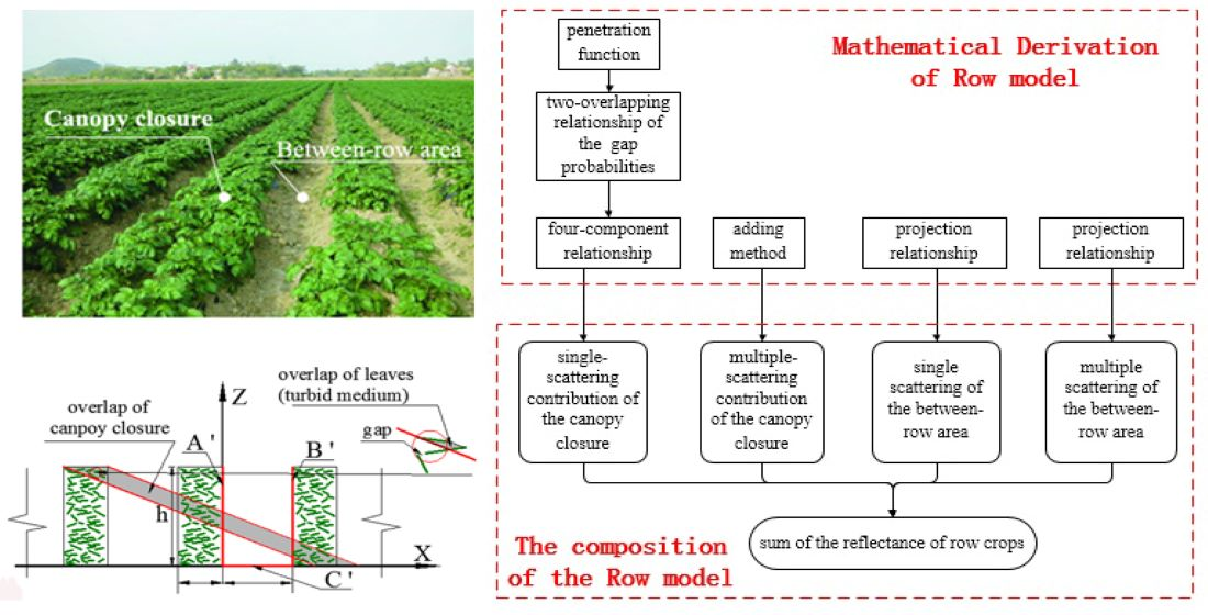
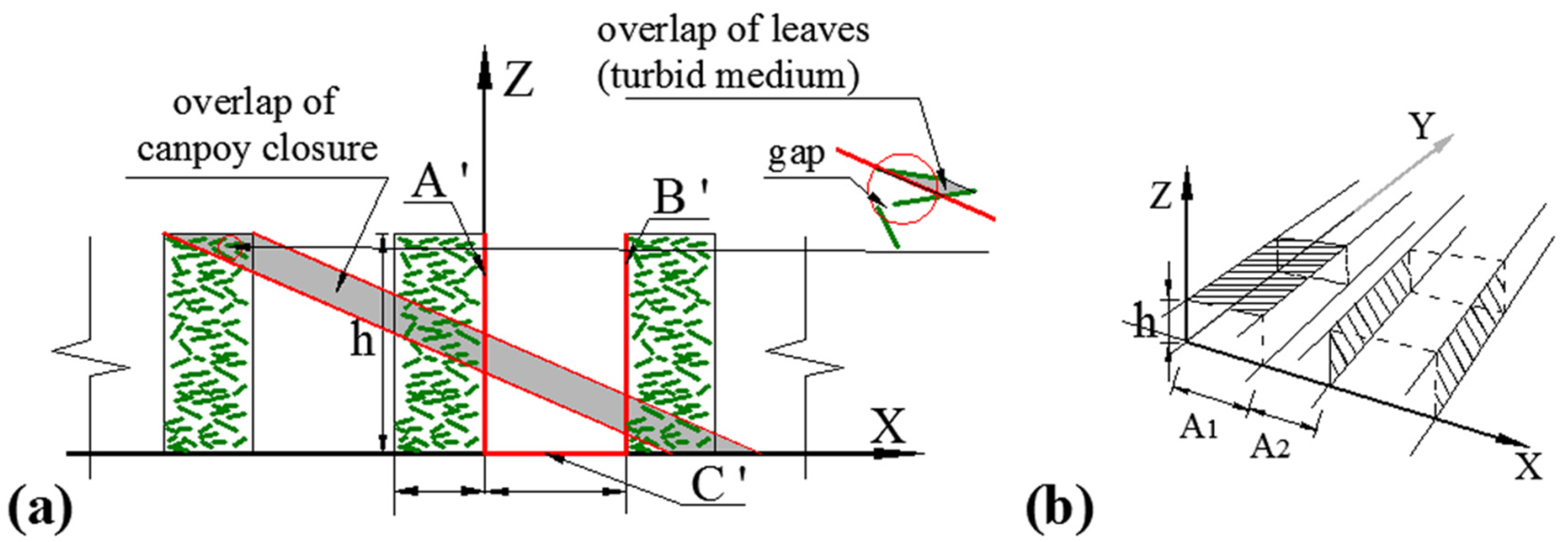
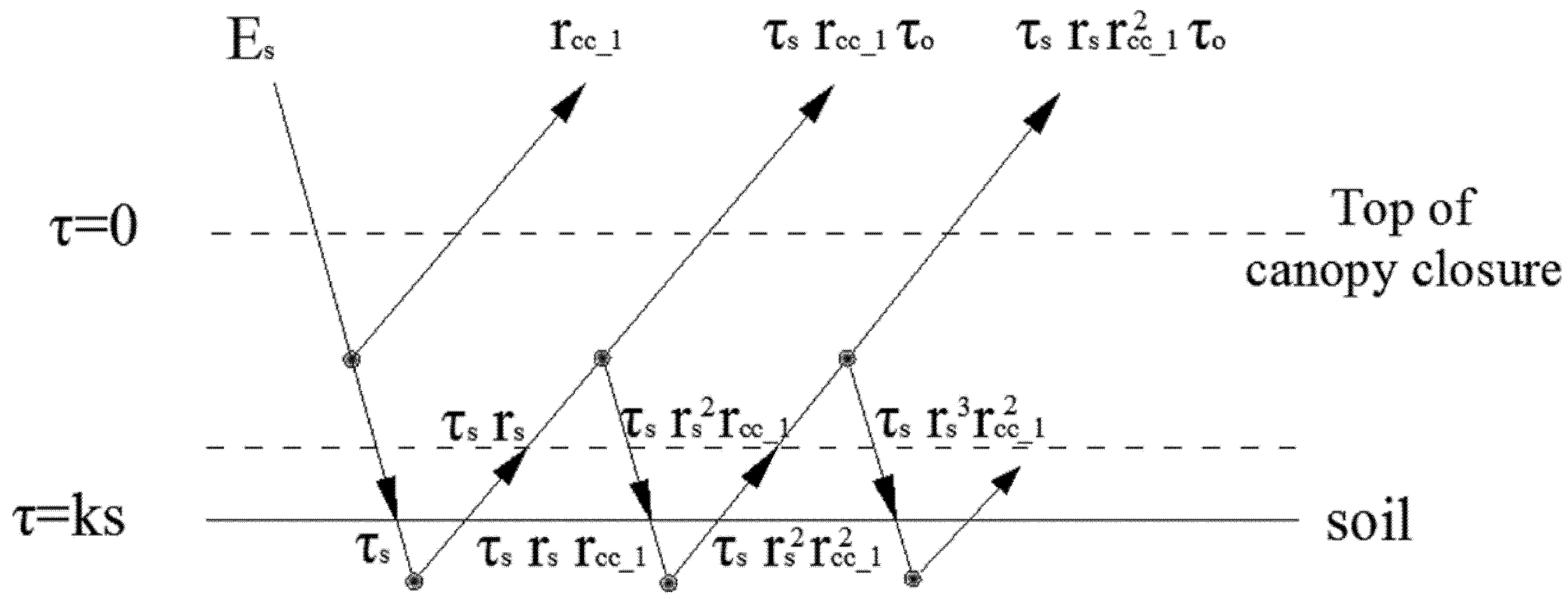
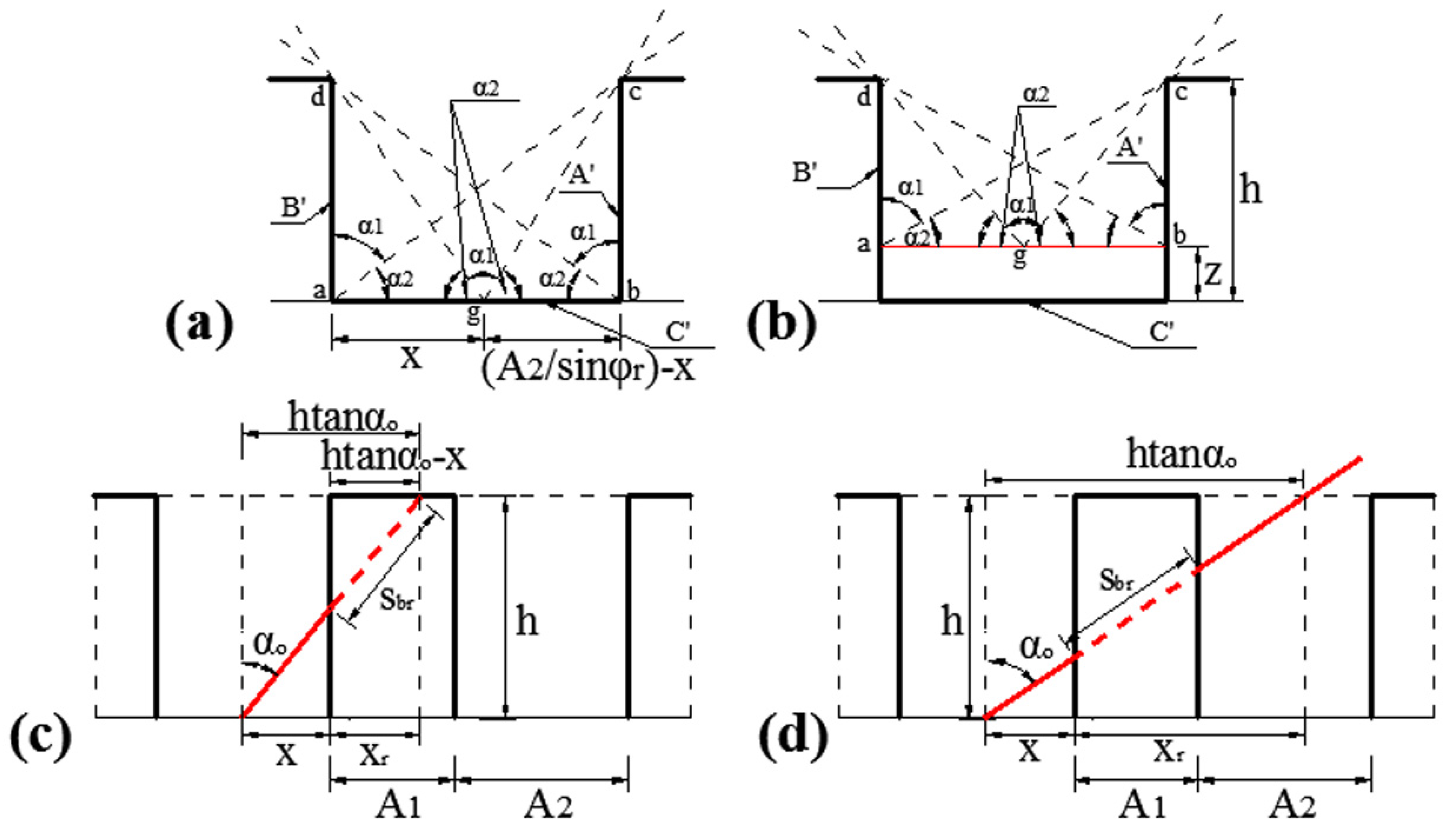
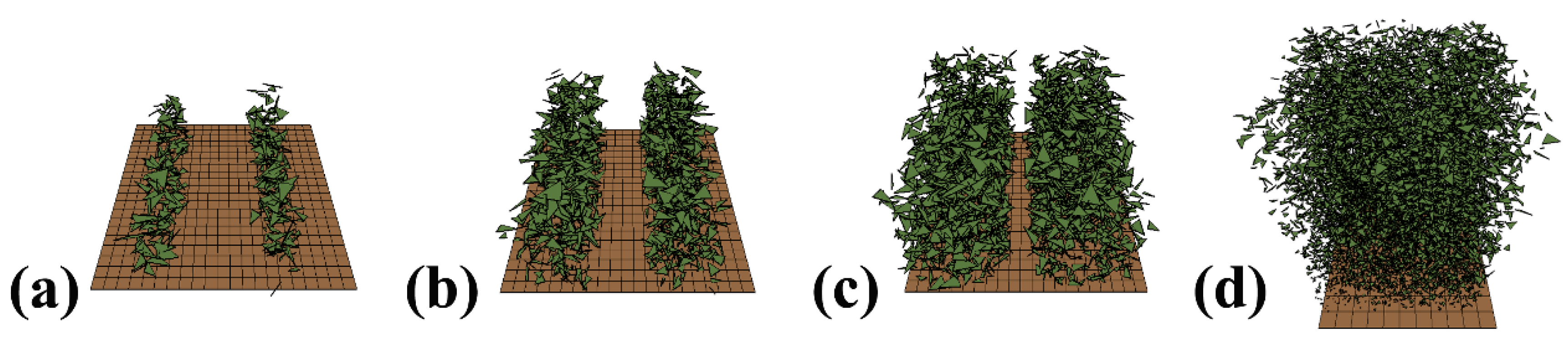
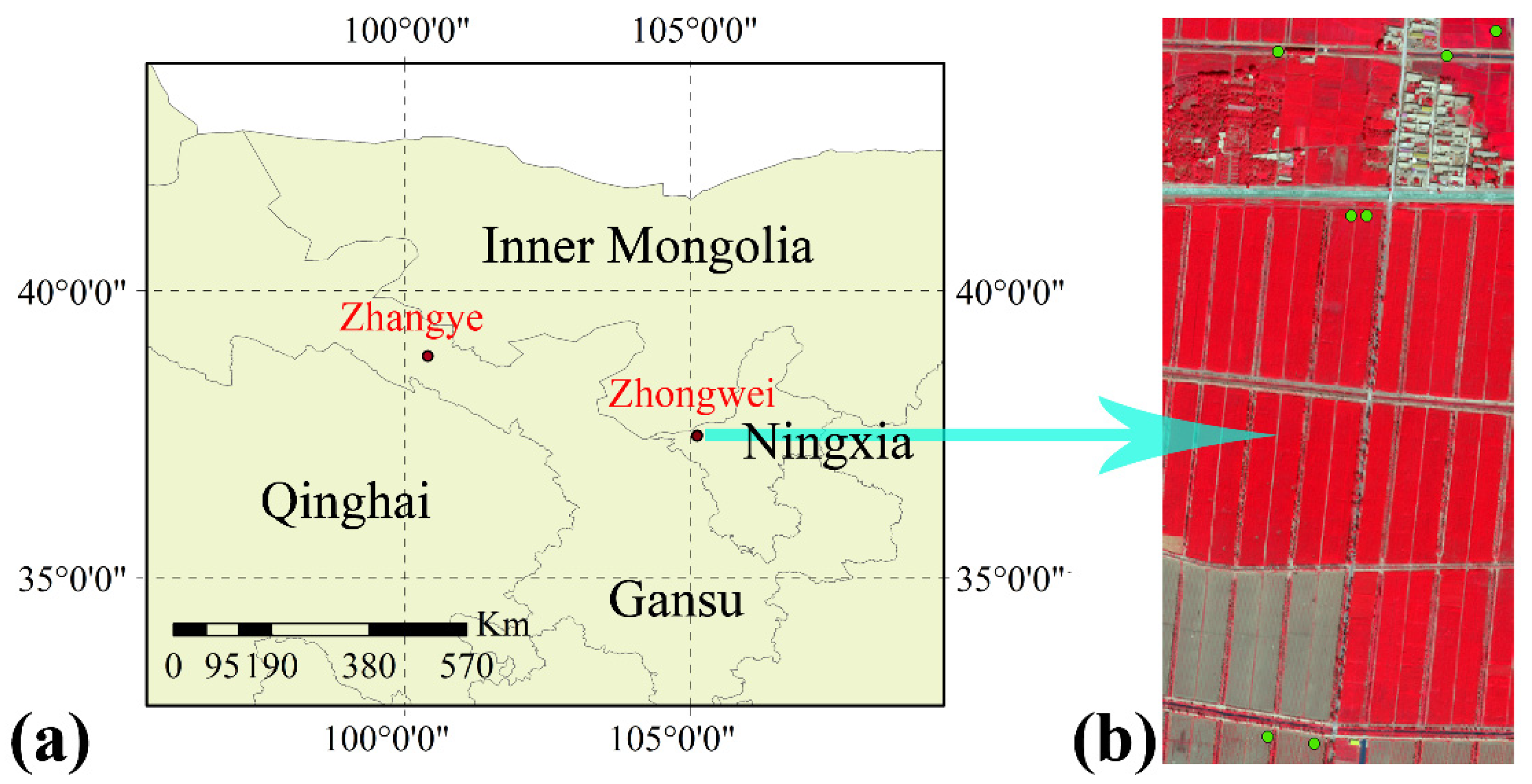
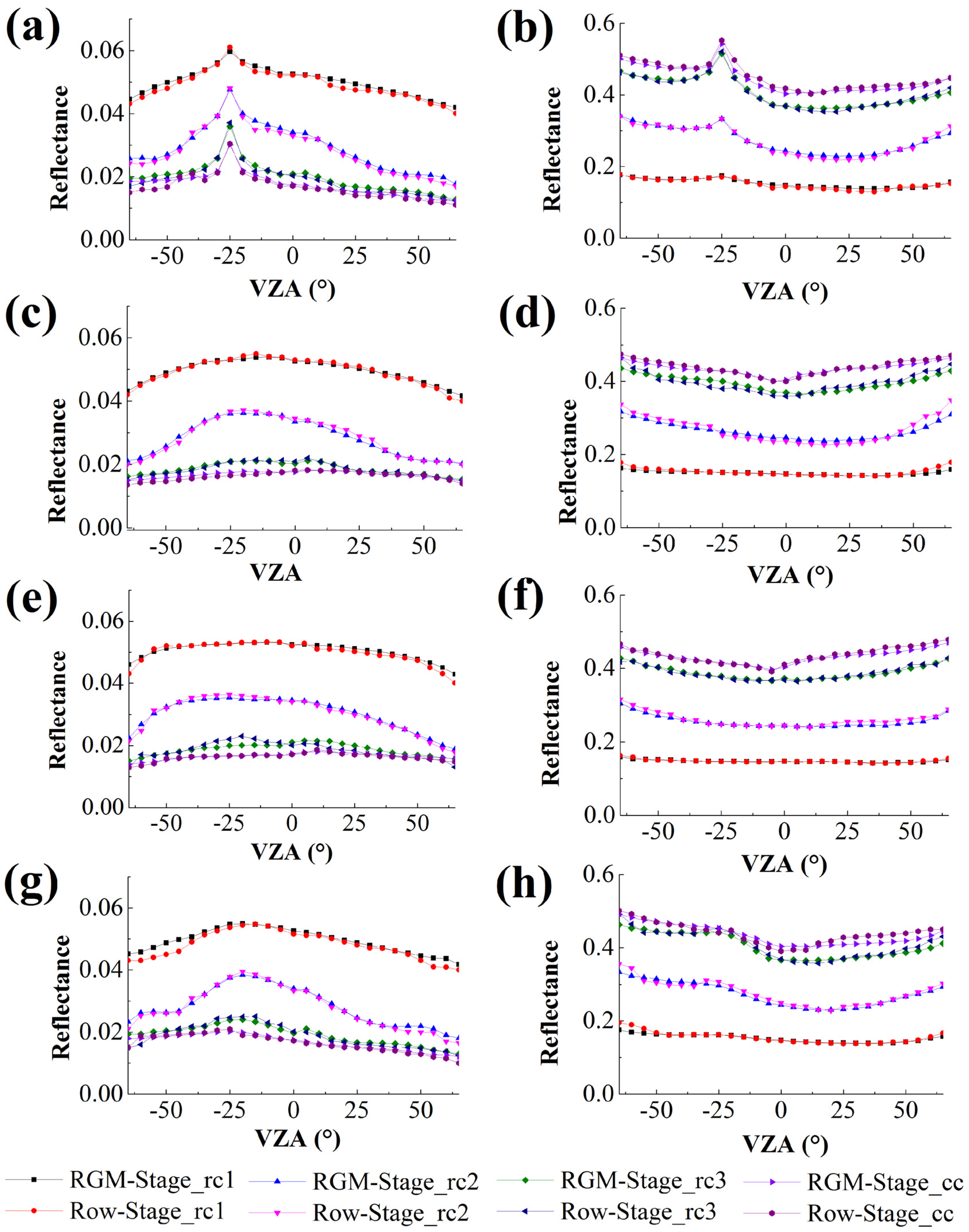
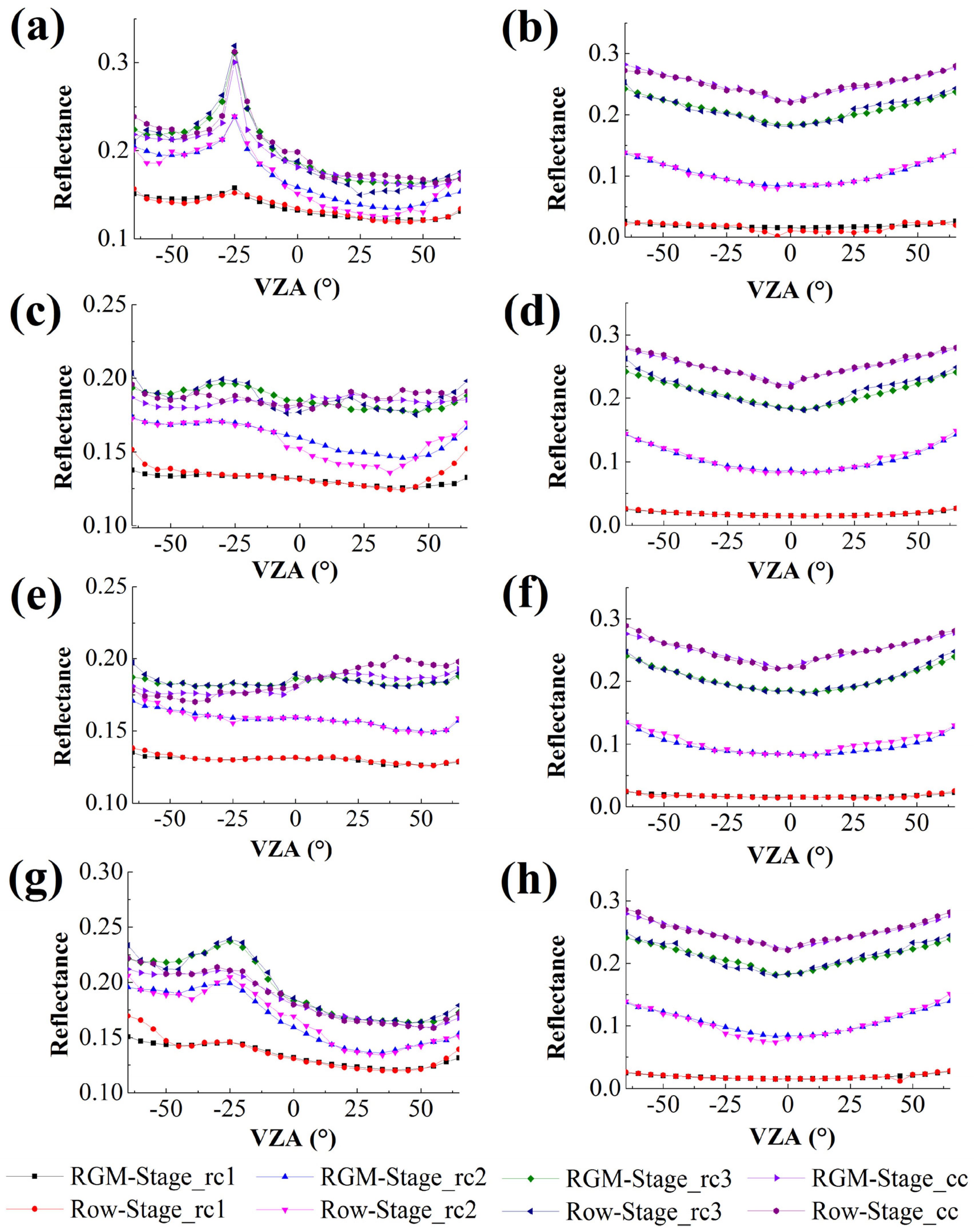
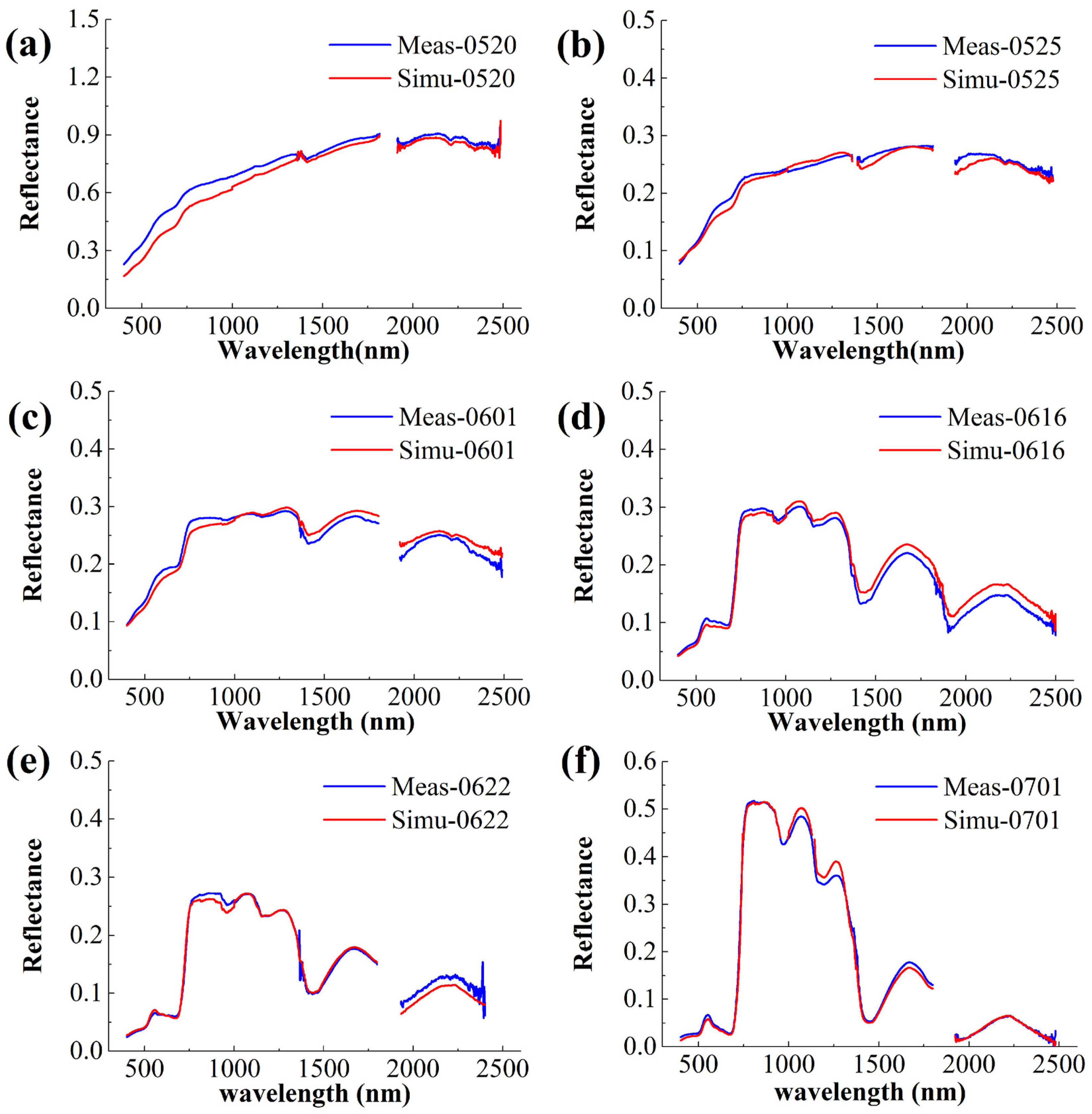
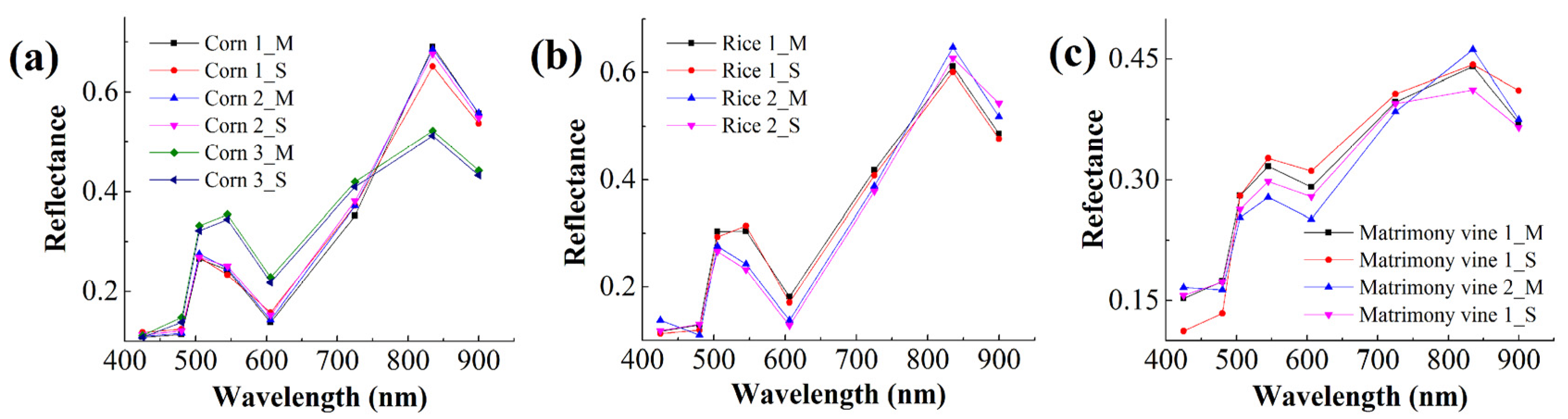
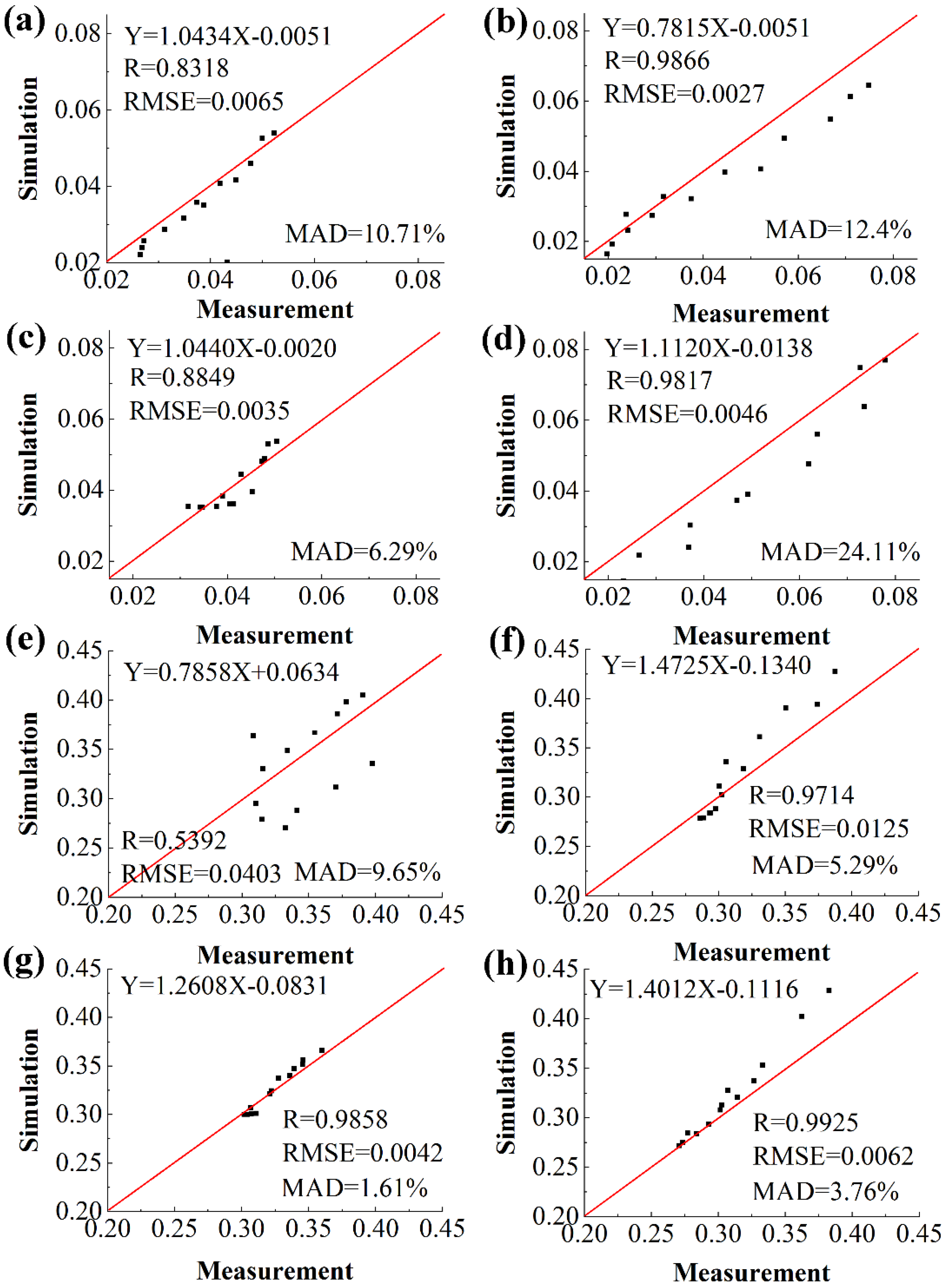
Table 1.
Values required when constructing abstract scenes with computer graphics.
| Scenes | L (m·m−1) | θl (°) 1 | A1 (m) | A2 (m) | H (m) | φr (°) | Wp (m) 1 |
|---|---|---|---|---|---|---|---|
| Stage_rc1 | 0.5 | 49.3 | 0.25 | 0.75 | 0.5 | 0 | 0.07 |
| Stage_rc2 | 1.5 | 43.4 | 0.5 | 0.5 | 0.8 | 0 | 0.07 |
| Stage_rc3 | 2.5 | 48.4 | 0.75 | 0.25 | 1.1 | 0 | 0.07 |
| Stage_cc | 3.5 | 46.7 | 1 | 0 | 1.4 | 0 | 0.07 |
1 Here, the inclined leaf angle and azimuth leaf angle are set to a random distribution. By counting the leaf inclination angle and width of the leaves for each polygon, we obtained the average leaf inclination angle (θl) and the characteristic width of leaves (Wp).
Table 2.
Structural parameters of corn in the growing season.
| Phenology | Date (2008) | L (m·m−1) | θl (°) | A1 (m) | A2 (m) | H (m) | φr (°) | Wp (m) |
|---|---|---|---|---|---|---|---|---|
| Emergence | 20 May | 0.23 | 49.16 | 0.2 | 0.80 | 0.16 | 110 | 0.03 |
| Emergence | 25 May | 0.34 | 48.15 | 0.25 | 0.75 | 0.22 | 110 | 0.04 |
| Jointing stage | 1 June | 0.46 | 48.15 | 0.30 | 0.70 | 0.35 | 110 | 0.07 |
| Jointing stage | 16 June | 1.76 | 40.83 | 0.5 | 0.5 | 0.87 | 110 | 0.08 |
| Jointing stage | 22 June | 2.52 | 59.0 | 0. 65 | 0.35 | 0.98 | 110 | 0.13 |
| Jointing stage | 1 July | 4.52 | 37.83 | 0.85 | 0.15 | 1.54 | 110 | 0.14 |
Table 3.
Structural parameters of crops in the quadrats.
| Quadrats | L (m·m−1) | θl (°) | A1 (m) | A2 (m) | H (m) | φr (°) | Wp (m) |
|---|---|---|---|---|---|---|---|
| Corn 1 | 3.19 | 45.33 | 0.9 | 0.4 | 2.66 | 40 | 0.16 |
| Corn 2 | 3.54 | 44.67 | 0.91 | 0.29 | 2.63 | 40 | 0.18 |
| Corn 3 | 2.6 | 32.00 | 0.99 | 0.2 | 2.82 | 45 | 0.14 |
| Rice 1 | 3.18 | 59.00 | 0.42 | 0.12 | 0.68 | 50 | 0.02 |
| Rice 2 | 3.17 | 63.67 | 0.3 | 0.13 | 0.78 | 53 | 0.04 |
| Matrimony vine 1 | 1.25 | 36.25 | 1.29 | 1.03 | 1.2 | 43 | 0.01 |
| Matrimony vine 2 | 0.77 | 68.33 | 1.04 | 0.93 | 0.86 | 42 | 0.01 |
Table 4.
The statistical results of the comparison of curves of reflectance simulated by the row model versus the reflectance simulated by the Radiosity–Graphics Combined Model (RGM) model.
Table 4.
The statistical results of the comparison of curves of reflectance simulated by the row model versus the reflectance simulated by the Radiosity–Graphics Combined Model (RGM) model.
| Scenes | Statistics | R_red | R_NIR | R_NIR_1 | R_NIR_m |
|---|---|---|---|---|---|
| Stage_rc1 | R | 0.9766 | 0.9282 | 0.8975 | 0.7972 |
| RMSE | 0.0009 | 0.0046 | 0.0043 | 0.0029 | |
| MAD | 1.98% | 1.87% | 1.86% | 9.82% | |
| Stage_rc2 | R | 0.9902 | 0.9612 | 0.9683 | 0.9731 |
| RMSE | 0.0009 | 0.0094 | 0.0056 | 0.0045 | |
| MAD | 3.08% | 2.99% | 2.58% | 3.54% | |
| Stage_rc3 | R | 0.9568 | 0.9678 | 0.9817 | 0.9754 |
| RMSE | 0.0011 | 0.0087 | 0.0048 | 0.0061 | |
| MAD | 4.64% | 1.68% | 1.81% | 1.93% | |
| Stage_cc | R | 0.9296 | 0.9601 | 0.9699 | 0.9850 |
| RMSE | 0.0009 | 0.082 | 0.0056 | 0.0031 | |
| MAD | 4.03% | 1.82% | 2.64% | 0.99% |
Publisher’s Note: MDPI stays neutral with regard to jurisdictional claims in published maps and institutional affiliations. |
© 2020 by the authors. Licensee MDPI, Basel, Switzerland. This article is an open access article distributed under the terms and conditions of the Creative Commons Attribution (CC BY) license (http://creativecommons.org/licenses/by/4.0/).
Share and Cite
MDPI and ACS Style
Ma, X.; Liu, Y. A Modified Geometrical Optical Model of Row Crops Considering Multiple Scattering Frame. Remote Sens. 2020, 12, 3600. https://0-doi-org.brum.beds.ac.uk/10.3390/rs12213600
AMA Style
Ma X, Liu Y. A Modified Geometrical Optical Model of Row Crops Considering Multiple Scattering Frame. Remote Sensing. 2020; 12(21):3600. https://0-doi-org.brum.beds.ac.uk/10.3390/rs12213600
Chicago/Turabian StyleMa, Xu, and Yong Liu. 2020. "A Modified Geometrical Optical Model of Row Crops Considering Multiple Scattering Frame" Remote Sensing 12, no. 21: 3600. https://0-doi-org.brum.beds.ac.uk/10.3390/rs12213600
Note that from the first issue of 2016, this journal uses article numbers instead of page numbers. See further details here.