Article

Reconstruction and Nowcasting of Rainfall Field by Oblique Earth-Space Links Network: Preliminary Results from Numerical Simulation

College of Meteorology and Oceanography, National University of Defense Technology, Nanjing 211101, China
*
Author to whom correspondence should be addressed.
Remote Sens. 2020, 12(21), 3598; https://0-doi-org.brum.beds.ac.uk/10.3390/rs12213598
Submission received: 21 September 2020 / Revised: 23 October 2020 / Accepted: 28 October 2020 / Published: 2 November 2020
(This article belongs to the Section Atmospheric Remote Sensing)

Abstract

:
High-precision rainfall field reconstruction and nowcasting play an important role in many aspects of social life. In recent years, the rain-induced signal attenuation of oblique earth-space links (OELs) has been presented to monitor regional rainfall. In this paper, we set up the first OEL in Nanjing, China, for the estimation of rain intensity. A year of observations from this link are also compared with the measurements from laser disdrometer OTT-Parsivel (OTT), between which the correlation is 0.86 and the determination coefficient is 0.73. Then, the simulation experiment is carried out: an OELs network is built, and the Kriging interpolation algorithm is employed to perform rainfall field reconstruction. The rainfall fields of plum rain season from 2016 to 2019 have been reconstructed by this network, which shows a good agreement with satellite remote sensing data. The resulting root-mean-square errors are lower than 3.46 mm/h and spatial correlations are higher than 0.80. Finally, we have achieved the nowcasting of rainfall field based on a machine-learning approach, especially deep learning. It can be seen from experiment results that the motion of rain cell and the position of peak rain intensity are predicted successfully, which is of great significant for taking concerted actions in case of emergency. Our experiment demonstrates that the densely distributed OELs are expected to become a futuristic rainfall monitoring system complementing existing weather radar and rain gauge observation networks.

Graphical Abstract

1. Introduction

Precipitation is an important chain of the water cycle and its spatiotemporal distribution is closely related to nature disasters such as floods and drought [1]. The latest research suggests climate changes have significantly affected the variability and trends of precipitation in China [2]. In 2020, the city of Shanghai suffered its longest plum rain season in the recent two decades. Mishra et al. also indicated that the probability of compound flooding from extreme precipitation and storm surge will become higher because of climate change [3]. Therefore, high-resolution and accurate precipitation measurement is crucial to study and monitor this changing risk, which also has a great significance on a numerical weather prediction (NWP) model that heavily relies on its initial conditions [4].
Existing methods for precipitation observation mainly include the tipping-bucket rain gauges (TBRGs) network and weather radars (WRs) [5]. A rain gauge network can provide more accurate rain intensity at fixed locations in the monitoring region, but its spatial representativeness is not sufficient for the disaster warning especially in complex terrain [6,7]. The weather radar achieves regional quantitative precipitation estimations (QPEs) with higher spatiotemporal resolution [8]. However, the uncertainty of the relationship between radar reflectivity and rain intensity leads to the errors [9]. In mountain areas, the effects of beam blockage, ground clutter and bright band interception cannot be neglected [10,11]. Moreover, the cost of operation, maintenance, and management for above two monitoring systems is quite expensive.
In the applications of Internet of Things (IoT), the horizontal microwave links (HMLs) of commercial cellular communication networks has been suggested as an alternative approaches for near-ground precipitation monitoring [12,13]. Compared with rain gauges and weather radars, the reconstruction of rainfall field by HMLs network basically depends on the existing infrastructure, which has a relatively low cost [14]. The HMLs can be considered as passive rainfall detection sensors, and the power-law relation between rain intensity and rain attenuation is used to quantitatively estimate precipitation. Minda and Nakamura have demonstrated that the resolution of HMLs measurement is higher than that of the gauge network [15]. Many experiments have proven that this method is very useful to measure precipitation in support of existing observation systems [14,16,17]. Moreover, some studies have indicated that the links of commercial 5G networks can also be used to reconstruct a rainfall field [18]. In other applications, the HMLs have been employed to the classification of rainfall type, radar calibration and raindrop size distribution retrieval [19,20,21].
Inspired by the utilization of HMLs, the oblique earth-space links (OELs) between ground and satellite have been studied for rainfall monitoring [22,23,24,25]. As another source of microwave links, the deployment of the OELs rainfall observation system cannot only use the existing equipment but also has a lower installation cost [26]. One sensor typically comprises a low noise block downconverter (LNB) and a common dish antenna. Most of the published studies focus on the rain intensity inversion by geostationary earth orbit (GEO) satellites OELs. Barthes et al. made use of the Ku band OELs to detect rainfall in Paris, and the measurements were compared with rain gauge and weather radar. Their results demonstrated that the OELs are very useful in hilly areas where the radar data cannot be obtained [22]. Differently to the HMLs, there are more complex atmospheric factors, such as gas, cloud, turbulence and melting layer, affecting the rainfall inversion by OELs [27]. In our previous work, we analyzed the characteristics of signal variation and proposed a novel approach to address two critical issues in OEL rainfall inversion: the identification of rain-no-rain period and the determination of signal reference level [28].
In addition to GEO satellites, there are nearly two thousand low earth orbit (LEO) and medium earth orbit (MEO) satellites operating in space. In the near future, more MEO/LEO satellites will be launched to build satellite constellations such as SpaceX and OneWeb which aim to provide global Internet services [29,30]. In order to make the service commercially available, the use-cost must be at a lower price. Compared with GEO satellites, the earth-space links of MEO/LEO satellites scan the rainfall field in a vertical direction. Based on this characteristic, some researchers have proposed to detect the precipitation in different heights by using MEO/LEO OELs [31,32]. Moreover, the preliminary experiment results from Xi’s work demonstrated that the LEO OELs have a great potential for 3-D precipitation reconstruction based on tomography techniques [6]. In practice, there are so many factors needing to be considered, such as the variation of hydrometeor phase which leads to different relations between hydrometeor and signal attenuation [33].
Therefore, this article mainly focuses on the 2-D near surface rainfall field reconstruction by GEO OLEs network, and some experiments are carried out to indicate its feasibility and reliability. So far, there have been few researches on rainfall field reconstruction by the OELs network [34,35,36]. In 2015, Mercier et al. built four Ku band OELs in the Vivarais region in the south of France and reconstructed the rainfall field based on a four-dimensional variational data assimilation (4DVAR) method [35]. Due to the limitation of algorithm, their model had a poor performance on the rainfall events with strong advection and is restricted to short events that are less than 45 min in length. In 2020, a network consisting of 37 OELs has been deployed in the City of Genoa (Italy) by Colli. et al. [36]. The measurements of main rainfall events between January 2017 and December 2018 were compared with TBRGs and WR. Their results showed 10-min rain intensity is consistent with WR and peak rain intensity as well as total accumulated rain which has a good agreement with TBRGs.
Furthermore, the nowcasting for instantaneous heavy rainfall has been a hot topic in meteorological fields because it is significantly important for relevant department to take timely actions for sudden natural disasters alerts such as flash floods and mudslides. To the best of our knowledge, no one else has done this work by using the OELs network. Inspired by the work of Shi who achieved the extrapolation of radar echo based on the machine learning [37], we design a deep learning network to discuss the feasibility of rainfall nowcasting by using the OELs network. The aim of our work is to carry out a preliminary attempt to achieve reasonable rainfall prediction over a relatively short period of time based on OELs network measurements:
In this paper, our contributions mainly include:
(1)
Large spatial region. The reconstruction of rainfall field with 1×1 km2 resolution is performed in the Jiangning district of Nanjing, China, whose area is approximately 1225 km2. The experimental results show the great potential of the OELs network in large scale rainfall monitoring.
(2)
Lots of data validations. Except for the validation of rain intensity inversion by a single link, the performance of the OELs network for rainfall field reconstruction is validated by using the satellite data during the plum rain season from 2016 to 2019.
(3)
Accurate rainfall field prediction. The designed deep learning network is used to achieve rainfall field nowcasting based on the observations of the OELs network. In validation experiment, the sequential change of rainfall field is predicted successfully.
The paper is organized as follows. The field measurement of rainfall from OEL is presented in Section 2. The reconstruction of rainfall field and corresponding simulation experiment are given in Section 3. A deep learning network is designed to achieve the nowcasting of the rainfall field in Section 4. We further discuss the performance of the OELs network on rainfall field reconstruction in Section 5. The main conclusions of this article are drawn in Section 6.

2. Field Measurement of Mainfall from OEL

2.1. Inversion of Rain Intensity by a Single OEL

For a single OEL, the received signal power Pr is related to the power of satellite transmitter Pe, the gain of antennas ηG, the free-space power loss ηF, the tropospheric attenuation ηT and the power of noise Pn, which can be written as:
P r ( t ) = η G ( t ) η F ( t ) η T ( t ) P e ( t ) + P n ( t )
where the ηT refers to the attenuation caused by rainfall ηR and other atmospheric factor ηO such as oxygen, water vaper, liquid water in cloud and scintillation. Therefore, in terms of the signal to noise ratio (SNR), its expression in decibels can be given by:
S N R ( t ) = 10 log η G ( t ) η O ( t ) P e ( t ) P n ( t ) A R ( t ) A F ( t )
where AR and AF are the rainfall- and free-space attenuation in decibels, respectively. As for the noise power Pn, it can be described as:
P n ( t ) = k B B T s y s ( t ) + T s k y ( t )
where kB is the Boltzman’s constant, B is the bandwidth of OEL signal, Tsys and Tsky denote the noise temperature of receiving system and sky. During rainy period, the sky noise collected by antenna mainly derives from rainfall. The corresponding noise power is related to the rain intensity and antenna directivity. Because the sampling period of satellite signal is very short in our experiment (about 6 s), it is reasonable to assume that the change of Tsys, ηG and Pe is negligible. Therefore, the Equation (2) can be rewritten as:
S N R ( t ) = V ( t ) F n ( t ) A R ( t ) A F ( t )
where Fn is defined as Equation (5), and if we know the Tsys, the Fn will only relate to Tsky. Moreover, the change of V mainly depends on the attenuation caused by no-rain factor and its expression is given by Equation (6).
F n ( t ) = 10 log T s y s + T s k y ( t ) T s y s
V ( t ) = 10 log η G η O ( t ) P e P 0
where P0 is written as:
P 0 = k B B T s y s
For a fixed solid angle Ω, the relation between the sky noise temperature Tsky(Ω) and rain attenuation in this direction is described as [38]:
T s k y ( t , Ω ) = t m 1 10 A R ( t ) 10
where tm is the path-average temperature. Considering the effect of antenna beam, the received sky noise can be expressed by [38]:
T s k y ( t ) = G ( t , Ω ) T s k y ( t , Ω ) d Ω G ( t , Ω ) d Ω
where the G(t, Ω) is the antenna gain for a particular direction. Therefore, the sky noise Tsky is a function of rain attenuation AR. Moreover, the free-space attenuation AF relates to the signal frequency and the distance from satellite to antenna. The specific relation among them can refer to literature [39]. For a GEO earth-space link, the value of AF is assumed as a constant.
According to ITU-R P.838 [40], the rain specific attenuation γrain is a function of rain intensity R in a power-law manner that is:
γ r a i n = α R β A R = γ r a i n h 0 + 0.36 / sin θ
where the coefficients α and β relate to signal frequency, polarization, temperature, and raindrop size distribution, θ is the elevation of antenna and h0 is the height of 0 °C isotherm. Most of existing studies on rainfall inversion by OLE depend on this relation.
During the no-rain period, the value of SNR is given by:
S N R n o r a i n = V ( t ) F n ( t ) A F ( t )
where we consider this value as a reference level SNRrefer that is used to obtain the rain attenuation. In our previous work, the issue, determining reference level during rain period has been addressed [28]. According to Equations (4) and (11), the rain attenuation can be expressed by:
A R ( t ) = S N R r e f e r ( t ) S N R r a i n ( t )
Therefore, based on the Equations (10) and (12), we can retrieve the path-average rain intensity R ¯ which is described as:
R ¯ = ( A R sin θ / ( ( h 0 + 0.36 ) α ) ) β 1

2.2. Experimental Setup

To assess the performance of rainfall inversion by OEL, a real earth-space link is established in the Jiangning district of Nanjing, China (31°58′27′′N, 118°48′52′′E). The signal of this link is obtained from AsiaSat 5 that is a GEO satellite located above 100.5°E and emits C- and Ku band signal towards east Asia. Furthermore, a dish antenna in 1.2 m diameter receives the 12.32 GHz with vertical polarization. Based on the received data, the values of SNR are estimated by the corresponding terminal which outputs the estimations once every 6 s for 24 h a day. Moreover, a modern laser disdrometer, OTT-Parsivel (OTT), is deployed near the antenna as a comparison. The OTT can measure the rain intensity with 1-min resolution. This link has been working since July 2019, and the rainfall measurements will be used to evaluate the feasibility and potential of OEL for rainfall field reconstruction.

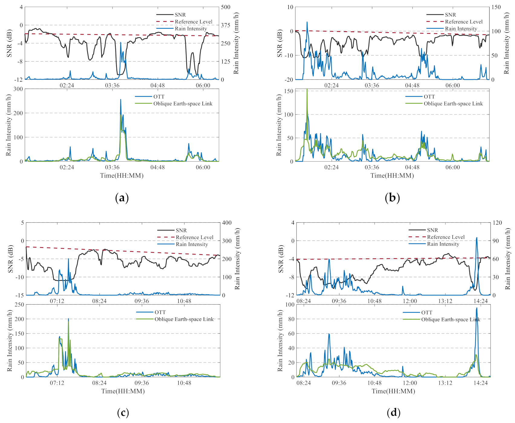
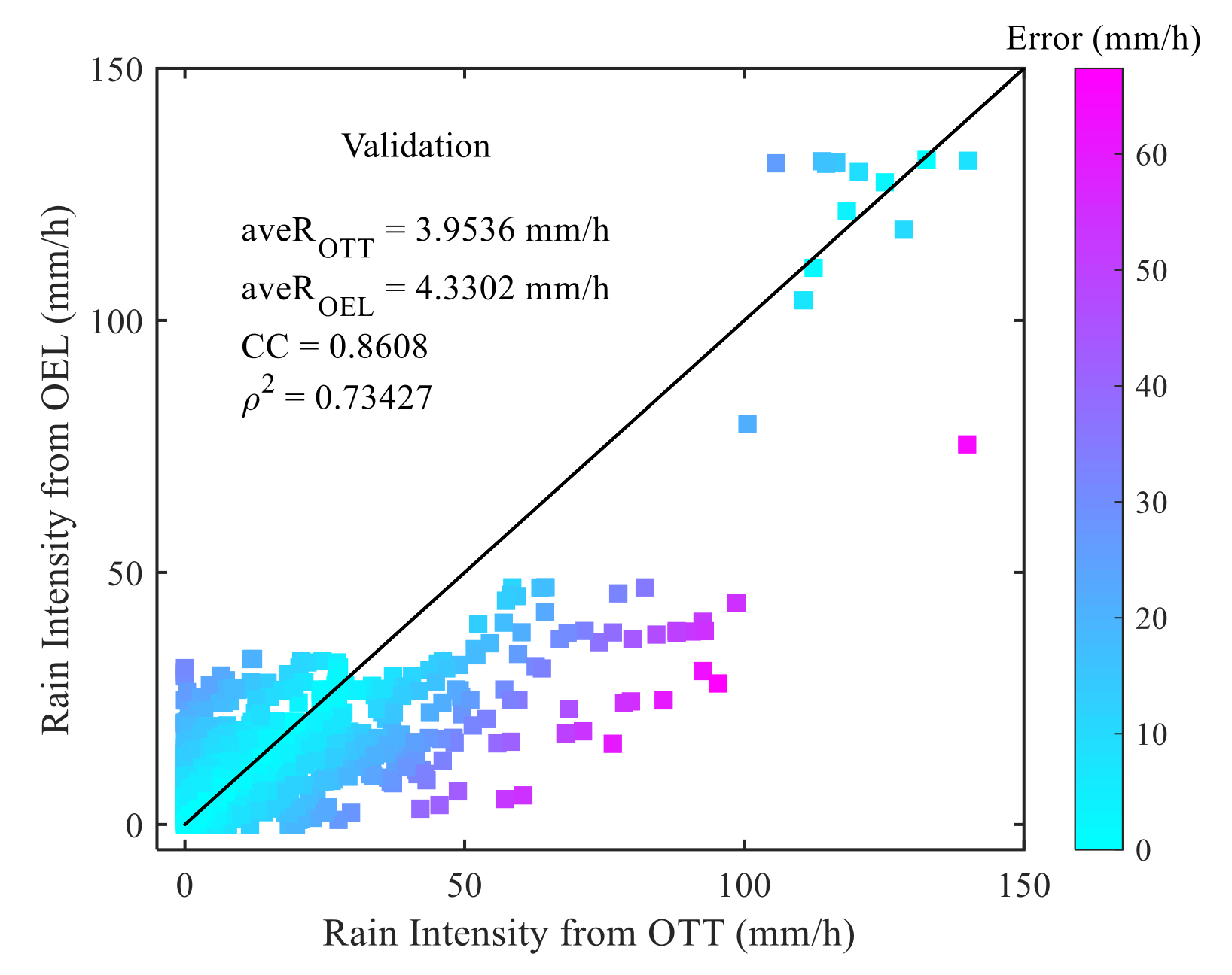
2.3. Validation of Rainfall Inversion

During the plum rain season in 2020, the continuous rainfall has caused serious floods in the Yangtze River basin of China. An extreme rainfall event occurred from June 13 to 16, 2020 and the maximum rain intensity has exceeded 200 mm/h. Next, we will analyze the performance of OEL in these days. The data used here are measured by our established OEL. The comparisons between SNR from receiving terminal and rain intensity from OTT are shown in upper part of each subplot of Figure 1. Due to the limitation of OTT, the temporal resolution of SNR is changed to 1 min. It can be clearly observed that the SNR are negatively correlated with rain intensity and the correlation coefficient (CC) between them is approximately −0.615. Moreover, the inversed rain intensity from OEL is also shown in the lower part of each subplot. In comparison with OTT measurements, the results of OEL show a good agreement, especially for June 13 and June 15. For the given four examples, the temporal correlations between OTT and OEL are higher than 0.68 and root mean square error (RMSE) is lower than 12 mm/h. Although the above results cannot accurately describe the actual performance of OEL, they indicate the potential of OEL being used to reconstruct the rainfall field. Moreover, we will evaluate the rainfall inversion by OEL based on a year of data in Section 5.

3. Reconstruction of Rainfall Field by OELs Network

3.1. Reconstuction Algorithm

In this paper, we reconstruct the rainfall field by establishing an OELs network. Firstly, each OEL measures the rain intensity at the corresponding position (xi, yi) based on the method in Section 2. Secondly, the rainfall measurements by all OELs are used to reconstruct the rainfall field. Here, the ordinary kriging interpolation algorithm (OK) is adopted. It is assumed that the rain intensity in observed region are related to each other, and the closer locations have much stronger correlations [41]. As for the target position (xt, yt) where the OELs are not deployed, its rain intensity R(xt, yt) can be estimated by:
R ( x t , y t ) = i = 1 n λ i R ( x i , y i ) i = 1 n λ i = 1
where the R(xi, yi) is the measured rain intensity by OELs at (xi, yi), n denotes the number of OEL measurements, λi is the weight that represents the contribution of R(xi, yi) to R(xt, yt). To obtain the weights, we need to solve a system of linear equations given by [42]:
γ 11 γ 12 γ 1 n 1 γ 21 γ 22 γ 2 n 1 γ n 1 γ n 2 γ n n 1 1 1 1 1 0 λ 1 λ 2 λ n φ = γ 1 t γ 2 t γ n t 1
where φ is the Lagrange’s multiplier, and vij is the semi-variance between Ri and Rj.
γ i j = 1 2 E R ( x i , y i ) R ( x j , y j ) 2
In the application of OK interpolation, it considers that semi-variance is a function of the distance and direction between observation- and target position. Its usual formula is:
γ ^ h = 1 2 M ( h ) i = 1 M ( h ) [ R ( x i ) R ( x i + h ) ] 2
where R(x) is the rain intensity at position x, R(x+h) is the value at (x+h), h is the separation in both distance and direction and not the actual position, and the M(h) is the number of pairs of observations separated by the lag h. Here, the function that γ relates to h is the variogram used to describe the variation within limited neighborhoods. Because the variation of rainfall field is generally considered isotropic, h only represents the lag distance of the experimental variogram. In the computer process, we choose a variogram model, like gaussian, spherical or stable, and fit it based on the OEL observations. The selection of variogram model will be discussed in Section 5 and this paper uses the stable model to reconstruct rainfall field [42].

3.2. Simulation Experiment

To prove the feasibility of the above methods to reconstruct the rainfall field, a simulation experiment has been carried out in Jiangning district. We choose five broadcast satellites to build the OELs network, and the architecture is shown in Figure 2a. To avoid the effect of different power-law relations, the chosen satellites have similar frequencies. The corresponding quantities and parameters are tabulated in Table 1. Considering the heterogeneity of rain intensity in the monitored region, we divide the rainfall field into 35 × 35 grid cells with 1 × 1 km2 resolution (as shown in Figure 2b). According to existing studies, we suppose the rain intensity in each cell is uniform, and the change of rainfall in vertical direction is not considered [36]. Therefore, the path-integrated rain attenuation of kth OEL is described as:
A R ( k ) = h 0 L sin θ i = 1 N γ i d i
where the N is the number of the grid cells traveled through by kth OEL, L denotes the horizontal projection of link on the ground and di is the projection of OEL on ith grid cell. Here, it is assumed that the height of 0 °C isotherm is well known as statistical value of Nanjing equal to 4.67 km. Because the inversed rain intensity is a path-averaged value, we convert it into data point at the middle position of link which is denoted as the blue “×” in Figure 2b. In this work, the synthetic rainfall field are derived from the data given by the Climate Prediction Center morphing method (CMORPH) of NOAA [43]. This technique can provide half-hourly global precipitation estimates, which combines the high-quality values derived from LEO satellite passive microwave (PMW) observations with propagation vector matrices obtained from successive GEO satellite infrared radiation (IR) images.
Moreover, a typical pencil beam antenna pattern is used to calculate the sky noise temperature [44]. We only consider nine sample directions comprising a main direction of antenna beam center and eight directions that are symmetrically around the center. Four of them are 0.6° away from the main direction and the remaining four are taken away 1.2°. The values of antenna gain in the eight directions are −10 dB and −20 dB, respectively. Based on Equation (9), the sky noise temperature is obtained by:
T s k y = T 0 + i = 1 4 0.1 T i + i = 5 8 0.01 T i 1 + 4 × 0.1 + 4 × 0.01
where Ti is the sky noise temperature in each sample direction which is calculated by Equation (8). In addition, it is assumed system noise temperature Tsys and path-average temperature tm are equal to 150 K and 275 K, respectively [38,45]. Then the noise figure Fn can be given by Equation (5). According to the literature [39], the free-space attenuation AF of the OELs in Jiangning district is between 205.77 and 206.16 dB. We suppose the V has a sinusoidal variation from 244 to 246 dB which simulates the effect of other atmospheric factors [46,47]. Based on Equation (4), the true SNR is obtained.
In practice, the signal-to-noise ratio is estimated by receiver system and denoted as S N R ^ . A maximum likelihood estimator is deployed in signal process terminal to estimate SNR [48]. The expected value and variance of S N R ^ are given by:
S N R ^ = 2 W 2 W 3 S N R + 1 2 W var ( S N R ^ ) = 2 ( 2 W ) 2 ( 2 W 3 ) 2 ( 2 W 5 ) 2 S N R 2 + 2 S N R 1 1 W + 1 2 W 1 1 W
where W is the number of data symbols used for SNR estimation. The bit rate of received signal is set as 10 Mbps [49]. Considering the bias of estimated signal-to-noise ratio and the relative error of measured rain attenuation, a Gaussian random variable n is added to true rain attenuation AR. Therefore, the measured attenuation A R ^ is expressed as:
A R ^ = A R + n n ~ N ( 0 ,   var ( S N R ^ )   ±   0.01 A R )
where 0.01 AR represents 1% relative error in measured rain attenuation. Therefore, the path-average rain intensity of OELs can be calculated, and then the rainfall field will be reconstructed by using the ordinary kriging (OK) model. The simulation process of rainfall field reconstruction is shown in Figure 3.

3.3. Performance of Rainfall Field Reconstruction

We perform the reconstruction of rainfall field based on the OK and inverse distance weighting (IDW) interpolation, respectively. The corresponding results are compared with CMORPH rainfall fields to assess the performance of the OELs network. The comparisons of four rainfall maps are shown in Figure 4 where the first line is the synthetic field from CMORPH, the second and the third lines are the reconstructed fields based on the IDW and OK, respectively. Although we can roughly observe the peak and distribution of rain intensity from reconstructed fields by IDW, the results based on OK show a better agreement with synthetic field and the crucial characteristics of rainfall field are also described accurately. In addition, Table 2 provides evaluation metrics of the reconstructed fields. Here, CC indicates the spatial correlation of two rainfall fields and S denotes the entropy used to represent the heterogeneity of rain intensity and its expression is given by:
S = 1 ln n m i = 1 n j = 1 m R i j F ln R i j F F = i = 1 n j = 1 m R i j
where n and m are the number of grid cell in horizontal and vertical directions.
In terms of the four given examples, the results derived from OK algorithm are more accurate whose RMSE is lower than 1 mm/h. It also can be seen from the values of CC that the reconstructed- and synthetic field are strongly correlated with each other whose value is higher than 0.89. Although the entropy S of IDW and OK rainfall fields are both close to synthetic field, showing similar distributions of rain intensity, the results of OK are still better than IDW. Based on above simulations, we achieve the reconstruction of rainfall field by OELs network. The results also demonstrate that the OK interpolation method used in our work is better at addressing this issue than IDW which is adopted in other relevant studies. Although the simulation only achieves the reconstruction of rainfall field in the Jiangning district whose area is approximately 1225 km2, the results indicate the feasibility and great potentials of widely distributed OELs for national or even global rainfall monitoring. On the other hand, the terrain of Jiangning is mainly plain and the effects of topography need to be considered in practice. To prevent the surface multipath fading and distortion, OEL is generally sited where significant specular and diffuse surface reflections rarely occur and many techniques have been proposed to address this issue [50]. As for the region where we cannot employ a lot of OELs, the interpolation algorithm used in this article shows obvious advantages.

4. Nowcasting of Rainfall Field

4.1. Nowcasting of Rainfall Field Based on Deep Learning

Based on the reconstructed rainfall fields by an OELs network, it is possible to predict the local regional rainfall over a relatively short period of time (e.g., several hours). In this article, we propose a deeplearning-based method to achieve the high spatiotemporal resolution nowcasting of rainfall field. The structure of our designed learning network is shown in Figure 5 and we can observe that the network comprises seven different layers where N denotes the number of sequential rainfall fields used in the training set.
For the sequence input layer, it receives the rainfall fields of training set and then transfers them into next layer in order. The 2D convolutional layer uses a 3 × 3 convolution kernel to extract the distribution features of rain intensity and the element in each feature matrix Ct can be described as:
C t ( i , j ) = p = 1 S q = 1 S A ( p , q ) R t ( i p + 1 , j q + 1 ) 1 i W R S + 1 1 j H R S + 1
where t is the tth rainfall field sample in training set, S is equal to 3 and denotes the size of convolution kernel A, Rt is the rain intensity of rainfall field, WR and HR are the number of columns and rows of rainfall field, respectively. Because the excessive number of elements in the feature matrix Ct may lead to extra training time and poor learning results, a 2D pooling layer is employed to reduce the number and meanwhile retains the main spatial information, the element of new feature matrix Dt is:
D t ( i , j ) = max ( B * C t ( 1 S + S i : S i , 1 S + S j : S j ) ) 1 i W C / S 1 j H C / S
where S is equal to 3 and denotes the size of sampling kernel B, C is the feature matrix, WC and HC denote the number of columns and rows of feature matrix, respectively. Then each feature matrix Dt is reshaped as one-dimension vector xt and then transferred into Long Short-Term Memory (LSTM) block in time sequence. As can be seen that an output vector ht (also known as the hidden state) is generated at each time step t which reflects the spatiotemporal property of rainfall field, and the calculation of ht is:
i t = σ g W x i x t + W h i h t 1 + b i f t = σ g W x f x t + W h f h t 1 + b f g t = σ c W x g x t + W h g h t 1 + b g o t = σ g W x o x t + W h o h t 1 + b o c t = f t c t 1 + i t g t h t = o t σ c c t
where i, f, g and o denote the input-, forget-, update- and output gate, respectively, and the functions of them can refer to literature [51]; ct represents the cell state; σg and σc are the hyperbolic tangent- and sigmoid activation function. Then, ht as an input is transferred to fully connected layer that aims to establish the mapping relation between ht and the rain intensity vector rt+1 of target rainfall field in the next time step:
r t + 1 = W h t + b
where W and b are the weight matrix and bias vector, respectively. Here, as rt+1 is reshaped to a two-dimension matrix, it denotes the predicted rainfall field Rt+1,p in t+1 time step. Finally, based on the errors between predictions and measurements, the regression layer iteratively adjusts the parameters in LSTM and fully connected layers to make the below loss function (Equation (27)) meet the terminal condition.
l o s s = 1 2 N t = 1 N j = 1 H R W R R t + 1 , m ( j ) R t + 1 , p ( j ) 2
where Rt+1,m and Rt+1,p denote the rain intensity of predicted- and measured rainfall field at t+1 time step, respectively. Here, the terminal condition is loss < 0.01 or reaching maximum iteration.

4.2. Result of Rainfall Field Nowcasting

In this section, we try to achieve the nowcasting of rainfall field by using our designed learning network. We select 386 rainfall events from CMORPH measurements between 2016 and 2019 to generate a dataset, which comprises 2649 sequential rainfall fields. In this article, the selection of rainfall events follows two principles:
(1)
Long duration. Because the time interval of CMORPH measurements is only 30 min, a shorter duration may not reflect the detailed spatiotemporal change of rain intensity in a rainfall event. The duration of selected rainfall event exceeds 4 h which means that an event includes at least eight continuous rainfall fields.
(2)
Heavy rainfall intensity. The aim of this work is to achieve the nowcasting of heavy rainfall that closely relates to instantaneous natural disaster, whose intensity is higher than 10 mm/h according to the WMO Guide to Meteorological Instruments and Methods of Observation (WMO-No.8, the CIMO Guide). Therefore, the maximum rain intensity in each rainfall event is higher than 10 mm/h.
In addition, the optimizer employed in the training process is an adaptive moment algorithm (Adam) and the initial learning rate is 0.02. To prevent gradient explosion and overfitting, the gradient threshold is set as 1 and the learning rate drop factor is set as 0.5 after 300 iterations. The maximum number of iterations is 500.
Figure 6 shows the comparisons between predictions and measurements from the OELs network for two precipitation events (from top to bottom), where the first two lines are results of 31 May 2016 and the last two lines are results of 2 August 2016. Here, we only display five continuous predictions of each rainfall event (from left to right) because the duration (2.5 h) is enough for us to observe the change of rainfall field in time sequence. For the event of May 31, two rain cells move from south to north. According to the variation of rain intensity, we can clearly observe the development and weakening of the second rain cell after the first leaves the monitoring region. For the event of 2 August the centers of heavy rainfall grew from one to two and then gradually weakeneds. As can be seen from the comparisons, the motion of rain cell and the change of peak rain intensity are predicted successfully, which is of great significance for nature disaster alerts. The corresponding evaluation metrics are given in Table 3. As for the given two rainfall events, it can be found that the learning network has a good performance on the nowcasting of rainfall field with RMSE lower than 3.5 mm/h and CC higher than 0.77.
Table 4 is a contingency table, showing the skill score of our prediction method on heavy rainfall alarm for each grid cell in a monitored region [52]. In the table, TH denotes the number of grid cells with heavy rainfall that are predicted correctly, FH denotes the number of grid cells with R < 10 mm/h that are wrongly predicted as heavy rainfall, FN denotes the number of grid cells with R > 10 mm/h that are not alarmed successfully, and TN denotes the number of non-heavy rainfall grid cells that are predicted correctly. Proportion correct (PC) indicates the accuracy that the learning network predicts rainfall categories: heavy rainfall or not. Probability of detection (POD) reflects the probability of predicting heavy rainfall accurately. False alarm ratio (FAR) denotes the ratio that the non-heavy rainfall is mis-predicted. Frequency bias index (FBI) indicates the learning network is better at predicting heavy rainfall (>1) or not (<1), and FBI = 1 indicating similar ability to predict the two situations. As can be seen from Table 4, the heavy rainfall of each grid cell can be predicted with high accuracy (PC = 0.94, POD = 0.96, FAR = 0.051), and FBI = 1.01 indicates a slightly better ability to predict heavy rainfall. In total, our work provides a general framework for the nowcasting of rainfall field by the OELs network.
In the experiment, we also found that the learning network cannot give reasonable predictions for light rainfall (0~2.5 mm/h), especially at the initial state of precipitation. On the one hand, this is because the spatiotemporal features cannot be immediately picked up by the network. On the other hand, comparied to the temporal resolution of CMORPH, the duration of light rain event is not very long, which causes that a light rain event that just has a few rainfall maps. According to the selection principles, such samples are usually not selected into the dataset because they are hard to show the continuous change of rainfall field and easy to introduce extra errors for the prediction of heavy rainfall. Therefore, it is not enough for the learning network to get the characteristics of light rainfall events in the training process.

5. Discussion

5.1. The Evaluation of Rainfall Inversion from OEL

In this section, we will evaluate the performance of OEL on rainfall measurement based on a year of statistical rainfall data of our established OEL system, which has been collected since July, 2019. The comparisons of rain intensity between OEL and OTT are presented in Figure 7. Here, each data point denotes the values of rain intensity derived from the two devices at the same time and the corresponding color indicates its absolute error. As can be seen, the rain intensity from OEL is highly correlated with OTT and the correlation coefficient between them is 0.86. The determination coefficient ρ2 is used to evaluate the sensibility of OEL inversed result to the variation of real rain intensity (OTT) and it is defined as:
ρ 2 = 1 i = 1 N ( R O T T ( i ) R O E L ( i ) ) 2 / i = 1 N ( R O T T ( i ) R ¯ O T T ) 2
where N denotes the number of data points shown in Figure 7. In general, a high value of ρ2, equal to 0.73 here, indicates a good ability of OEL to measure rain intensity. The averages of rain intensity from OEL (4.33 mm/h) and OTT (3.95 mm/h) are also close to each other. In total, the OEL can achieve the measurement of rain intensity. However, we can clearly observe that the differences between OTT and OEL become more and more obvious with the increase of rain intensity. As for the extreme rain (50 mm/h~), the estimates from OEL are significantly lower than OTT. Therefore, we will further discuss the performance of OEL on different rainfall categories. The statistical relative errors between OEL and OTT for different rain intensity ranges are given in Figure 8. The medians of relative errors for rain intensity in 0~5 mm/h and 6~15 mm/h are 14.9% and −7.5%, respectively. With the increase of rain intensity, the medians exceed −20% and the worst value reaches to −41.3% for rain intensity in 31~50 mm/h. Above results demonstrate that the inversed rain intensity has better accuracy of light-(0~2.5 mm/h) and moderate-(2.5~10 mm/h) rain than that of heavy-(10~50 mm/h) and extreme rain.
As for the comparison between OEL and OTT, it should be noted that directly comparing the rain intensity from the two devices may be not reasonable. On the one hand, the observed volumes of atmosphere by OTT and OEL are different. As mentioned above, the inversed rain intensity of OEL represent the average rainfall along the link, but the OTT measures the rain intensity of a single point near the surface. The heavy- and extreme rain event often associates with obvious spatial heterogeneities, which results in the obvious underestimation from OEL. Therefore, several disdrometers will be deployed along the earth-space link in our near future work. On the other hand, as can be seen from Equation (13), the height of 0 °C isotherm also influences the inversion results. In the above experiment, we use the radiosonde data to estimate the height of 0 °C isotherm. However, the radio sounding is only performed twice a day which is not strictly consistent with OEL measurements so an alternative method is urgently needed.

5.2. The Stability of Reconstruction Method

In this section, we will discuss the stability of our method on the reconstruction of rainfall field. Here, the OELs network is used to reconstruct the rainfall fields of the Jiangning district in plum rain season (June, July) of 2016, 2017, 2018 and 2019 by numerical simulation. The number of reconstructed fields during these periods is 1376 and the corresponding results are shown as accumulated rainfall fields in Figure 9. As for the calculation of accumulated rainfall field, it is equal to the sum of all rain intensity fields and meanwhile multiplies the temporal resolution of CMORPH that is equal to 0.5h. It can be seen from the comparisons that the important characteristics of accumulated rainfall field are inversed accurately, such as the increasing (or decreasing) trend of accumulated rain and the maximum (or minimum) position. Table 5 presents four metrics to quantitatively evaluate the reconstructed results. The values of CC between the OELs network and CMORPH are higher than 0.97 which shows a strong spatial correlation. The values of RMSE that are lower than 4.1 mm indicate the accuracy of our reconstruction method. Furthermore, the absolute relative errors of maximum and average values in accumulated rainfall fields do not exceed 1.5% and 0.5%, respectively. Moreover, the values of RMSE of 1376 reconstructed rain intensity fields are lower than 3.4 mm/h and CC are higher than 0.80.
In this simulation, we use the OELs network to inverse rain intensity of approximately 1.7 × 10⁶ grid cells. The comparison between inversed- and original rain intensity is presented in Figure 10. It can be seen that the rain intensity from both sources show a good consistency, with CC and ρ2 equal to 0.995 and 0.989, respectively. The relative error of average rain intensity is 0.28%. In addition, we can clearly observe from the color bar in Figure 10 that the absolute error of inversed rain intensity is significantly lower than that in Figure 7, which indicates a better accuracy of the reconstruction method. According to the result of linear regression in Figure 10 (black line: y = 0.9793x + 0.0622), there still are slight underestimations for high rain intensity. To quantitatively assess the accuracy of OELs network estimations for different rainfall categories, Figure 11 gives the statistical relative errors between OELs network and CMORPH. In total, the medians of each box are close to zero, and the corresponding values from left to right are −0.13%, −0.60%, −0.59%, −0.58% and −0.72%, respectively, showing an obvious improvement to the results in Figure 8. This is because the representativeness of inversed rain intensity is different and our simulation is performed under some ideal assumptions such as knowing the height of 0 °C isotherm well and ignoring the variation of rainfall in vertical direction. Above results can demonstrate that the method used in this paper has a stable performance on rainfall field reconstruction, but there are still many effects to be considered in practical application.

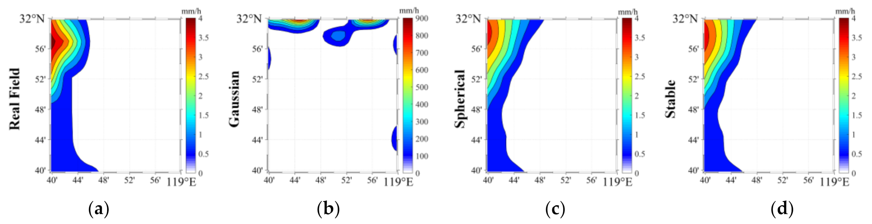
5.3. The Selection of Variogram Model

In this section, we will discuss the selection of variogram model that is used to reconstruct the rainfall field in this paper. The application of the OK algorithm is usually under an assumption that the distribution of property in observed field is close to Gaussian. According to the data used in Section 5.2, we can see that the rain intensity in our experimental region is an obvious non-Gaussian distribution (shown in Figure 12a) that the probability of light- and moderate rainfall is higher than heavy- and extreme rainfall. Therefore, it is necessary for us to find an approach to ensure the accuracy of reconstruction results. As we can see from Equation (17), the variogram model plays an important role in the OK algorithm because it directly relates to the calculation of λ in Equation (14). In non-Gaussian distributions, the variogram model may be sensitive to the field with high kurtosis or skewness. In Figure 12b,c, as the cumulative density function reaches to 0.9, the values of kurtosis and skewness are approximately equal to 10 and 2.5, respectively. Therefore, we will focus on the other 10% rainfall fields with high kurtosis and skewness to analyze the performances of different variogram models. Here, the gaussian-, spherical- and stable models are compared with each other and their expressions are [42]:
G a u s s i a n :   γ h = c 1 exp h r 2
S p h e r i c a l : γ h = c 3 2 h r 1 2 h r 3   if   0 h r , γ h = c   if   h > r .
S t a b l e : γ h = c 1 exp h r α
where c denotes the sill that represents the maximum value of the fitted variogram, and r denotes the range distance as γ reaching to c. It is noted that the formula of stable model is like gaussian model but has an unknown exponent α that needs to be fitted. A good performance of spherical model has been proved by Overeem et al. who achieved the reconstruction of rainfall field by using microwave links [17].
In Figure 13, the gray point denotes the measured semi-variance from OELs network, and the values of each rainfall field are scaled into [0, 1] to show the total change trend of semi-variance. The normalization can reduce effects caused by the magnitude of rain intensity. Here, the data of rainfall in May, August and September of 2016, 2017, 2018 and 2019 is added into that used in Section 5.2 because the rainfall in Nanjing is mainly concentrated in these five months. The solid lines in this figure denote the fitted variogram functions and the vertical lines represent the average absolute error between fitted- and measured value in each lag distance. It can be seen that the changes of the semi-variance of these four years are very similar to each other. As for the averages of unnormalized values of these four years, the correlation coefficients among them are higher than 0.996 and the standard errors are lower than 2.8 mm2/h2. The result indicates that the variogram of rainfall field in our experimental region has an almost invariable form. In each subplot, we can observe that all above three variogram models can represent the change trend of semi-variance whose determination coefficients are higher than 0.97 and the average absolute errors are lower than 0.15. It is hard to judge which model is better only according to the consistency with measured data.
Therefore, the rainfall fields with high kurtosis and skewness are used to test the three models. Here, 296 examples are selected from the above dataset and those rainfall maps all describe a similar situation that rainfall occurs only at the border of the experimental region. Figure 14 shows an example and the rainfall maps are reconstructed by using different models. The gaussian variogram gives the worst result that is far from a real situation. The results of spherical- and stable models are close to each other. The corresponding correlation coefficients are 0.98 and 0.97. The values of RMSE are 0.152 mm/h and 0.189 mm/h. In the experiment, we found that the performance of the gaussian model is not good on the field with high kurtosis but also not good in general situations. By contrast, the spherical- and stable models have higher stability. As for the selected 296 examples, the performance of stable model is slightly better whose correlation coefficient is higher than 0.76 and RMSE is lower than 1.92 mm/h.

6. Conclusions

In this paper, we propose a new approach that using an oblique earth-space links (OELs) network achieves the reconstruction and nowcasting of rainfall field. With the widely distributed links, the OELs network has a great potential to become a futuristic rainfall monitoring system. Meanwhile, based on the deep learning, we have preliminarily achieved the nowcasting of rainfall field by using OELs network.
To discuss the potential of using the OELs network in the application of rainfall field monitoring and prediction, we have set up an earthspace link in Nanjing, China to receive the 12.32 GHz vertically polarized signal from AsiaSat5. The resulting measurements are compared with the data from a modern laser disdrometer, OTT-Parsivel (OTT), which is co-located with receiving antenna. Then we select an extreme rainfall event in the plum rain season of 2020 to test this link, and a year of observations are also used to evaluate its performance. Then a monitoring network including 40 receiving antenna and 93 links are deployed in the Jiangning district of Nanjing. Combing it with the data from Climate Prediction Center morphing method (CMORPH), an interpolation method, ordinary kriging (OK), is employed to the reconstruction of rainfall field. To validate its stability and accuracy, we analyze its performance during the plum rain season of 2016, 2017, 2018 and 2019. Based on the machine learning approach, especially deep learning, we design a learning network to achieve the prediction of reginal rainfall over a relatively short period of time. Then 386 rainfall events from 2016 to 2019 are used to train learning network. A general conclusion can be drawn from this paper that the OLEs network is expected to become a new precipitation monitoring system in support of the existing TBRGs and WR observation network. The more specific conclusions are summarized as follows:
(1)
For the rainfall inversion by a single OEL, the results have a good agreement with OTT measurements. In terms of the extreme rainfall event from June 13 to 16, 2020, the RMSE is lower than 12 mm/h and CC is higher than 0.68. According to a year of statistical measurements, the inversion results have a reliable performance which associates with higher values of CC (0.86) and ρ2 (0.73). However, the OLE often underestimates the peak rain intensity of heavy- and extreme rainfall because its observation space is different from OTT and the height of the 0 °C isotherm is not known well.
(2)
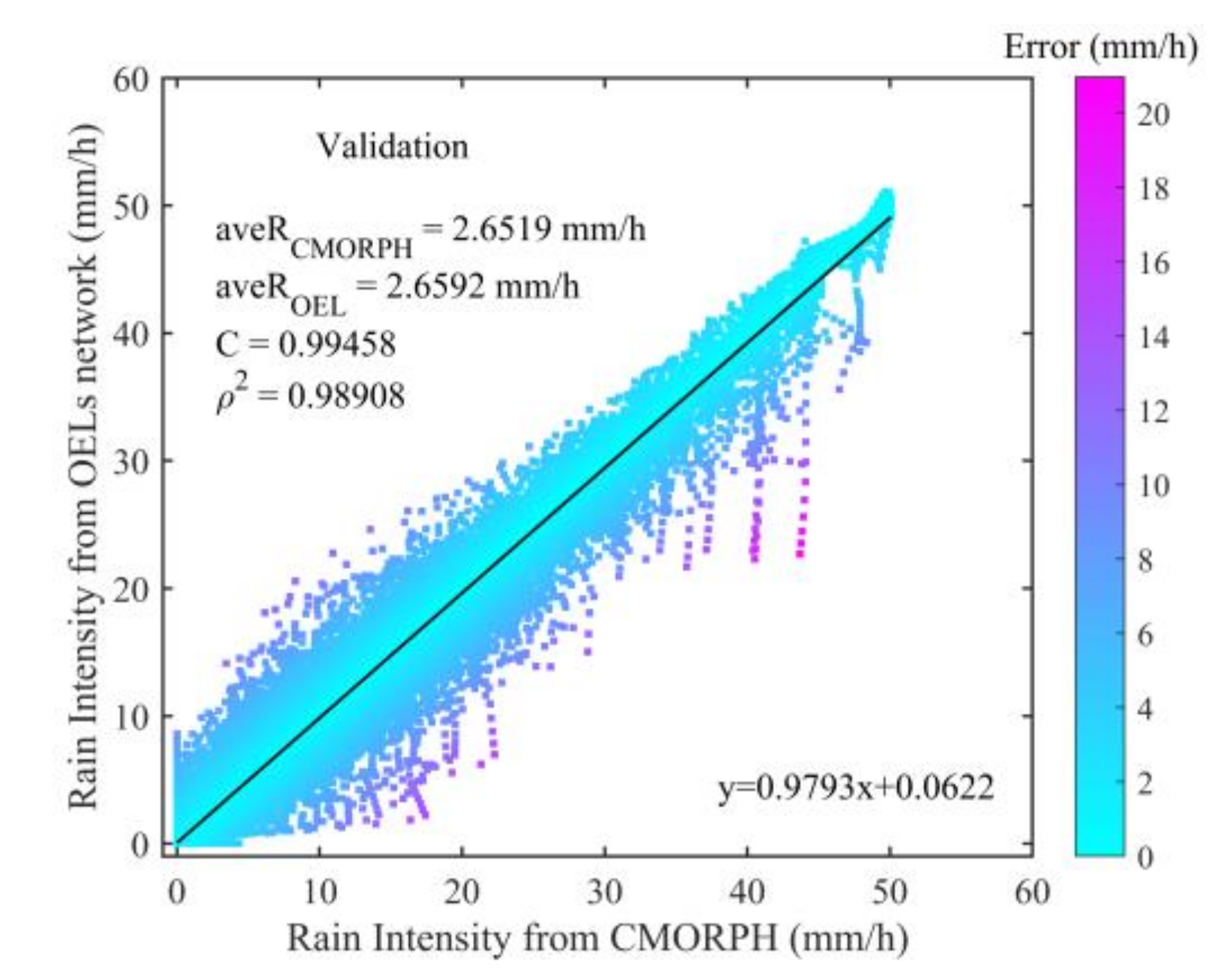
For the reconstruction of rainfall field, inversed results are strongly correlated with the measurements from CMORPH. It can be seen from the performances of OELs network during plum rain season of 2016, 2017, 2018 and 2019 that the increasing (or decreasing) trend of accumulated rain and the position of maximum (or minimum) value are reproduced accurately. In total, the OELs network can give reliable reconstructed rainfall fields with RMSE lower than 3.46 mm/h and CC higher than 0.80.
(3)
For the nowcasting of rainfall field, the motion of rain cell and peak rain intensity are predicted successfully, which is of great significance for natural disaster alerts. For given two examples, the values of RMSE is lower than 3.5 mm/h and CC is higher than 0.77. It is also noted that the learning network has a poor performance on predictions for light rain events (0~2.5 mm/h) due to the lack of corresponding samples in the training set.
In our near future work, an OELs network will be built in Nanjing, China for the application of regional precipitation monitoring. Moreover, to further improve the performance of OELs network, we will also research on the temporal properties of precipitation fields such as Hurst-Kolmogorov process [53]. According to the conclusions from this article, several issues need to be addressed in practice:
(1)
Assessing the uncertainty caused by the representativeness of OEL inversed rain intensity. In the process of rainfall field reconstruction, we assume that the path-average rain intensity is equal to the value in the middle of link. This may be not reasonable for the cases when precipitation has significant spatial heterogeneity. The sophisticated tomography reconstruction techniques, such as simultaneous algebra reconstruction technique (SART) and compressed sensing (CS), can be considered.
(2)
Assessing the errors introduced by the melting layer attenuation. The frequency of OEL for rainfall inversion is usually in the Ku- or Ka-band. For the signal above 10 GHz, melting layer attenuation is comparable to path-integrated rain attenuation, especially for low elevation OEL whose propagation path in melting layer is relatively long. Therefore, the issue of distinguishing melting layer attenuation from that of precipitation, needs to be addressed.
(3)
Assessing the variance of the variogram model. It has been shown that the estimator of semi-variance often exhibits an obvious variability and so can give estimations with large uncertainty [54]. Therefore, it is necessary to find an advanced method to reduce this effect. For example, climacogram has a better performance than conventional autocovariance and variogram, which can give more accurate results by removing the bias from estimation [55].

Author Contributions

Conceptualization, M.X. and X.L.; methodology, M.X. and X.L.; resources, M.X. and K.S.; investigation, K.S.; supervision, T.G.; writing-original draft preparation, M.X; writing-review and editing, M.Y. and X.L.; funding acquisition, X.L. All authors have read and agreed to the published version of the manuscript.

Funding

This research was funded by the National Natural Science Foundation of China, grant number 41975030, 41505135 and 41475020.

Acknowledgments

The authors would like to thank the editor and anonymous reviewers for their helpful comments and suggestions. The data measured by our established oblique earth-space link and laser disdrometer OTT can be supplied via request to the corresponding author of this manuscript. The data used in the simulation experiment on rainfall reconstruction and nowcasting is provided by Climate Prediction Center of NOAA which can be download from an open access https://ftp.cpc.ncep.noaa.gov/precip/CMORPH_V1.0/.

Conflicts of Interest

The authors declare no conflict of interest.

References

  1. Abbot, C. Precipitation Cycles. Science 1949, 110, 148. [Google Scholar] [CrossRef] [PubMed]
  2. Guo, B.; Zhang, J.; Meng, X.; Xu, T.; Song, Y. Long-term spatio-temporal precipitation variations in China with precipitation surface interpolated by ANUSPLIN. Sci. Rep. 2020, 10, 81. [Google Scholar] [CrossRef] [PubMed]
  3. Mishra, A.; Kumar, G. Climate change will affect global water availability through compounding changes in seasonal precipitation and evaporation. Nat. Commun. 2020, 11, 3044. [Google Scholar] [CrossRef]
  4. Alpert, P.; Rubin, Y. First Daily Mapping of Surface Moisture from Cellular Network Data and Comparison with Both Observations/ECMWF Product. Geophysical Res. Lett. 2018, 45, 8619–8628. [Google Scholar] [CrossRef]
  5. McCabe, M.F.; Rodell, M.; Alsdorf, D.E.; Miralles, D.G.; Uijlenhoet, R.; Wagner, W.; Lucieer, A.; Houborg, R.; Verhoest, N.E.C.; Franz, T.E.; et al. The Future of Earth Observation in Hydrology. Hydrol. Earth Syst. Sci. 2017, 21, 3879–3914. [Google Scholar] [CrossRef] [PubMed] [Green Version]
  6. Liu, X.; He, B.; Zhao, S.; Hu, S.; Liu, L. Comparative measurement of rainfall with a precipitation micro-physical characteristics sensor, a 2D video disdrometer, an OTT PARSIVEL disdrometer, and a rain gauge. Atmos. Res. 2019, 229, 100–114. [Google Scholar] [CrossRef]
  7. Zeng, Q.; Zhang, Y.; Lei, H.; Xie, Y.; Gao, T.; Zhang, L.; Wang, C.; Huang, Y. Microphysical Characteristics of Precipitation during Pre-monsoon, Monsoon, and Post-monsoon Periods over the South China Sea. Adv. Atmos. Sci. 2019, 36, 10. [Google Scholar] [CrossRef]
  8. Matrosov, S.Y. Dual-frequency radar ratio of nonspherical atmospheric hydrometeors. Geophys. Res. Lett. 2005, 32, 1–4. [Google Scholar] [CrossRef] [Green Version]
  9. Ulbrich, C.; Lee, L. Rainfall Measurement Error by WSR-88D Radars due to Variations in Z R Law Parameters and the Radar Constant. J. Atmos. Ocean. Technol. 1999, 16, 1017–1024. [Google Scholar] [CrossRef]
  10. Germann, U.; Galli, G.; Boscacci, M.; Bolliger, M. Radar Precipitation Measurement in a Mountainous Region. Q. J. R. Meteorol. Soc. 2007, 132, 1669–1692. [Google Scholar] [CrossRef]
  11. Wagner, A.; Seltmann, J.; Kunstmann, H. Joint statistical correction of clutters, spokes and beam height for a radar derived precipitation climatology in southern Germany. Hydrol. Earth Syst. Sci. 2012, 16, 4101–4117. [Google Scholar] [CrossRef] [Green Version]
  12. Messer, H.; Zinevich, A.; Alpert, P. Environmental Monitoring by Wireless Communication Networks. Science 2006, 312, 713. [Google Scholar] [CrossRef] [Green Version]
  13. Fencl, M.; Rieckermann, J.; Schleiss, M.; Stransky, D.; Bares, V. Assessing the potential of using telecommunication microwave links in urban drainage modelling. Water Sci. Technol. 2013, 68, 1810–1818. [Google Scholar] [CrossRef] [PubMed]
  14. Overeem, A.; Leijnse, H.; Uijlenhoet, R. Retrieval algorithm for rainfall mapping from microwave links in a cellular communication network. Atmos. Meas. Tech. 2016, 9, 2425–2444. [Google Scholar] [CrossRef] [Green Version]
  15. Minda, H.; Nakamura, K. High Temporal Resolution Path-Average Rain Gauge with 50GHz Band Microwave. J. Atmos. Ocean. Technol. 2005, 22, 165–179. [Google Scholar] [CrossRef]
  16. Goldshtein, O.; Messer, H.; Zinevich, A. Rain Rate Estimation Using Measurements From Commercial Telecommunications Links. IEEE Trans. Signal Process. 2009, 57, 1616–1625. [Google Scholar] [CrossRef]
  17. Overeem, A.; Leijnse, H.; Uijlenhoet, R. Country-wide rainfall maps from cellular communication networks. Proc. Natl. Acad. Sci. USA 2013, 110, 2741–2745. [Google Scholar] [CrossRef] [Green Version]
  18. Han, C.; Huo, J.; Gao, Q.; Su, G.; Wang, H. Rainfall Monitoring Based on Next-Generation Millimeter-Wave Backhaul Technologies in a Dense Urban Environment. Remote Sensing 2020, 12, 1045. [Google Scholar] [CrossRef] [Green Version]
  19. Pu, K.; Liu, X.; Xian, M.; Gao, T. Machine Learning Classification of Rainfall Types Based on the Differential Attenuation of Multiple Frequency Microwave Links. IEEE Trans. Geosci. Remote Sens. 2020, 58, 6888–6899. [Google Scholar] [CrossRef]
  20. Song, K.; Liu, X.; Gao, T.; He, B. Raindrop Size Distribution Retrieval Using Joint Dual-Frequency and Dual-Polarization Microwave Links. Adv. Meteorol. 2019, 2019, 1–11. [Google Scholar] [CrossRef]
  21. Rahimi, A.R.; Holt, A.R.; Upton, G.J.G.; Krämer, S.; Redder, A.; Verworn, H.-R. Attenuation Calibration of an X-Band Weather Radar Using a Microwave Link. Am. Meteorol. Soc. 2006, 23, 395–405. [Google Scholar] [CrossRef]
  22. Barthès, L.; Mallet, C. Rainfall measurement from the opportunistic use of an Earth–space link in the Ku band. Atmos. Meas. Tech. 2013, 6, 2181–2193. [Google Scholar] [CrossRef] [Green Version]
  23. Colli, M.; Stagnaro, M.; Caridi, A.; Lanza, L.G.; Randazzo, A.; Pastorino, M.; Caviglia, D.D.; Delucchi, A. A Field Assessment of a Rain Estimation System Based on Satellite-to-Earth Microwave Links. IEEE Trans. Geosci. Remote Sens. 2019, 57, 2864–2875. [Google Scholar] [CrossRef]
  24. Mugnai, C.; Sermi, F.; Cuccoli, F.; Facheris, L. Rainfall Estimation with a Commercial Tool for Satellite Internet in KA Band: Model Evolution and Results. In Proceedings of the 2015 IEEE International Geoscience and Remote Sensing Symposium, Milan, Italy, 26–31 July 2015; pp. 890–893. [Google Scholar] [CrossRef]
  25. Giannetti, F.; Moretti, M.; Reggiannini, R.; Vaccaro, A. The NEFOCAST System for Detection and Estimation of Rainfall Fields by the Opportunistic Use of Broadcast Satellite Signals. IEEE Aerosp. Electron. Syst. Mag. 2019, 34, 16–27. [Google Scholar] [CrossRef]
  26. Giannetti, F.; Reggiannini, R.; Moretti, M.; Adirosi, E.; Baldini, L.; Facheris, L.; Antonini, A.; Melani, S.; Bacci, G.; Petrolino, A.; et al. Real-Time Rain Rate Evaluation via Satellite Downlink Signal Attenuation Measurement. Sensors 2017, 17, 1864. [Google Scholar] [CrossRef]
  27. Dissanayake, A.; Allnutt, J.; Haidara, F. A prediction model that combines rain attenuation and other propagation impairments along Earth-satellite paths. IEEE Trans. Antennas Propag. 1997, 45, 1546–1588. [Google Scholar] [CrossRef]
  28. Xian, M.; Liu, X.; Yin, M.; Song, K.; Zhao, S.; Gao, T. Rainfall Monitoring Based on Machine Learning by Earth-space Link in the Ku Band. IEEE J. Sel. Top. Appl. Earth Obs. Remote Sens. 2020, 13, 3656–3668. [Google Scholar] [CrossRef]
  29. SpaceX. Starlink Mission. Available online: https://www.spacex.com/webcast (accessed on 20 March 2020).
  30. OneWeb. OneWeb. Available online: https://www.oneweb.world/ (accessed on 31 March 2020).
  31. Xian, M.; Liu, X.; Yin, M.; Song, K.; Gao, T. Inversion of vertical rainfall field based on earth-space links. Acta Phys. Sin. 2020, 69, 1–11. [Google Scholar] [CrossRef]
  32. Huang, D.; Xu, L.; Feng, X. A hypothesis of 3D rainfall tomography using satellite signals. J. Commun. Inf. Netw. 2016, 1, 134–142. [Google Scholar] [CrossRef]
  33. Mishchenko, M.I.; Travis, L.D.; Lacis, A.A. Scattering, Absorption, and Emission by Small Particle; Cambridge University Press: New York, NY, USA, 2002; p. 462. [Google Scholar]
  34. Mishra, K.V.; Gharanjik, A.; Shankar, M.R.B.; Ottersten, B. Deep Learning Framework for Precipitation Retrievals from Communication Satellites. In Proceedings of the 10th European Conference on Radar in Meteorology & Hydrology, Ede-Wageningen, The Netherlands; 2018; pp. 1–9. [Google Scholar]
  35. Mercier, F.; Barthes, L.; Mallet, C. Estimation of Finescale Rainfall Fields Using Broadcast TV Satellite Links and a 4DVAR Assimilation Method. J. Atmos. Ocean. Technol. 2015, 32, 1709–1728. [Google Scholar] [CrossRef] [Green Version]
  36. Colli, M.; Cassola, F.; Martina, F.; Trovatore, E.; Delucchi, A.; Maggiolo, S.; Caviglia, D.D. Rainfall Fields Monitoring Based on Satellite Microwave Down-Links and Traditional Techniques in the City of Genoa. IEEE Trans. Geosci. Remote Sens. 2020, 58, 6266–6280. [Google Scholar] [CrossRef]
  37. Shi, X.; Chen, Z.; Wang, H.; Yeung, D.-Y.; Wong, W.-K.; Woo, W.-C. Convolutional LSTM Network: A Machine Learning Approach for Precipitation Nowcasting. arXiv 2015, arXiv:1506.04214. [Google Scholar]
  38. Ho, C.; Slobin, S.; Gritton, K. Atmospheric Noise Temperature Induced by Clouds and Other Weather Phenomena at SHF Band (1-45 GHz). Available online: https://descanso.jpl.nasa.gov/propagation/Ka_Band/JPL-D32584_1.pdf (accessed on 15 July 2020).
  39. ITU. Recommendation ITU-R P.525-4 Calculation of Free-Space Attenuation; ITU: Geneva, Switzerland, 2019. [Google Scholar]
  40. ITU. Recommendation ITU-R P.838-3 Specific Attenuation Model for Rain for Use in Prediction Methods; ITU: Geneva, Switzerland, 2005. [Google Scholar]
  41. Dowd, P. The Variogram and Kriging: Robust and Resistant Estimators; Springer: Dordrecht, The Netherlands, 1983; Volume 1. [Google Scholar]
  42. Webster, R.; Oliver, M.A. Geostatistics for Environmental Scientist, 2nd ed.; WILEY: Hoboken, NJ, USA, 2008; p. 330. [Google Scholar]
  43. Joyce, R.; Janowiak, J.; Arkin, P.; Xie, P. CMORPH: A Method That Produces Global Precipitation Estimates From Passive Microwave and Infrared Data at High Spatial and Temporal Resolution. J. Hydrometeorol. 2004, 5, 487–503. [Google Scholar] [CrossRef]
  44. Mahajan, M.; Jyoti, R.; Sood, K.; Bhushan, S. A Method of Generating Simultaneous Contoured and Pencil Beams From Single Shaped Reflector Antenna. IEEE Trans. Antennas Propag. 2013, 61, 5297–5301. [Google Scholar] [CrossRef]
  45. Warnick, K.F.; Ivashina, M.V.; Maaskant, R.; Woestenburg, B. Unified Definitions of Efficiencies and System Noise Temperature for Receiving Antenna Arrays. IEEE Trans. Antennas Propag. 2020, 58, 2121–2125. [Google Scholar] [CrossRef]
  46. Singh, M.S.J.; Hassan, S.I.S.; Ain, M.F.; Igarashi, K.; Tanaka, K.; Iida, M. Analysis of Tropospheric Scintillation Intensity on Earth to Space in Malaysia. Am. J. Appl. Sci. 2006, 3, 2029–2032. [Google Scholar] [CrossRef]
  47. ITU. Recommendation ITU-R P.679-4 Propagation Data Required for the Design of Broadcasting-Satellite Systems; ITU: Geneva, Switzerland, 2015; pp. 1–6. [Google Scholar]
  48. Rm, G.; Cm, T. PCM Data Reliability Monitoring Through Estimation of Signal-to-Noise Ratio. IEEE Trans. Commun. Technol. 1968, 16, 479–486. [Google Scholar] [CrossRef]
  49. Reimers, U. Digital video broadcasting. IEEE Commun. Mag. 1998, 36, 104–110. [Google Scholar] [CrossRef]
  50. ITU. Recommendation ITU-R P.530-17 Propagation Data and Prediction Methods Required for the Design of Terrestrial Line-of-Sight Systems; ITU: Geneva, Switzerland, 2017; pp. 1–57. [Google Scholar]
  51. Hochreiter, S.; Schmidhuber, J. Long short-term memory(LSTM). Nerual Comput. 1997, 9, 1735–1780. [Google Scholar] [CrossRef]
  52. Nurmi, P. Recommendations on the Verification of Local Weather Forecasts. In ECMWF Technical Memoranda; ECMWF: Shinfield Park, UK, 2003. [Google Scholar] [CrossRef]
  53. Koutsoyiannis, D.; Paschalis, A.; Theodoratos, N. Two-dimensional Hurst–Kolmogorov process and its application to rainfall fields. J. Hydrol. 2011, 398, 91–100. [Google Scholar] [CrossRef]
  54. Dimitriadis, P.; Koutsoyiannis, D. Climacogram versus autocovariance and power spectrum in stochastic modelling for Markovian and Hurst–Kolmogorov processes. Stoch. Environ. Res. Risk Assess. 2015, 29, 1649–1669. [Google Scholar] [CrossRef]
  55. Dimitriadis, P.; Koutsoyiannis, K.T.D.; Tyralis, H.; Kalamioti, A.; Lerias, E.; Voudouris, P. Stochastic investigation of long-term persistence in two-dimensional images of rocks. Spat. Stat. 2019, 29, 177–191. [Google Scholar] [CrossRef]
Figure 1. An extreme rainfall event occurred from June 13 to 16, 2020: (a) June 13, (b) June 14, (c) June, 15 and (d) June 16. The black line is the signal to noise ratio (SNR), the dark red dotted line is the reference level, the blue- and green line are the rain intensity measured by OTT-Parsivel (OTT) and earth-space links (OELs), respectively.
Remotesensing 12 03598 g001
Figure 2. The architecture of OELs network in Jiangning district: (a) original distribution of links, and (b) rainfall field divided by grid cells where the black line is the OEL and the blue mark denotes the position of inversed rain intensity.
Remotesensing 12 03598 g002
Figure 3. The simulation process of rainfall field reconstruction.
Remotesensing 12 03598 g003
Figure 4. The comparisons of reconstructed- and synthetic rainfall field: 17:00, 25 May 2019; 8:00, 29 June 2019; 23:00, 11 July 2019 and 1:00, 10 August 2019
Remotesensing 12 03598 g004
Figure 5. The architecture of deep learning network for the rainfall field nowcasting: the sequence input layer receives oblique earth-space link (OEL) measurements, the convolutional- and pooling layer extract the spatial feature of rainfall field, the Long Short-Term Memory (LSTM) layer learns the time-dependence of spatial feature vectors and fully connected layer as well as regression layer predicts the regional rainfall for the next time.
Remotesensing 12 03598 g005
Figure 6. The comparisons between predicted results and OELs network measurements for two precipitation events (from top to bottom): 31 May 2016 and 2 August 2016. Each event is performed five continuous predictions (from left to right).
Remotesensing 12 03598 g006
Figure 7. The comparisons of rain intensity between OTT and OEL: the color of each square indicates its corresponding absolute error.
Remotesensing 12 03598 g007
Figure 8. The statistical relative errors between OEL and OTT for different rain intensity ranges.
Remotesensing 12 03598 g008
Figure 9. The accumulated rainfall from Climate Prediction Center morphing method (CMORPH) and OELs network during plum rain season (June, July) of 2016, 2017, 2018 and 2019 in Jiangning district of Nanjing.
Remotesensing 12 03598 g009
Figure 10. The comparisons between inversed rain intensity of all grid cells derived from OELs network and original values from CMORPH during plum rain season (June, July) of 2016, 2017, 2018 and 2019.
Remotesensing 12 03598 g010
Figure 11. The statistical relative errors between OEL and CMORPH for different rain intensity ranges.
Remotesensing 12 03598 g011
Figure 12. The probability density function and cumulative density function of (a) rain intensity, (b) kurtosis and (c) skewness.
Remotesensing 12 03598 g012
Figure 13. The data of normalized semi-variance measured by OELs network and corresponding variogram models in (a) 2016, (b) 2017, (c) 2018 and (d) 2019.
Remotesensing 12 03598 g013aRemotesensing 12 03598 g013b
Figure 14. (a) A rainfall field with high kurtosis and reconstructed results by using (b) gaussian, (c) spherical and (d) stable models.
Remotesensing 12 03598 g014
Table 1. The parameters of broadcast satellites chosen to build OELs network.
SatellitesElevation (°)Azimuth (°)Frequency (GHz)α (\)β (\)Quantities (\)
ApStar731.524012.550.02871.111917
AsiaSat547.8721212.320.02671.127618
ChinaSat1051.7519512.590.02881.121616
AsiaSat952.6717412.520.02821.124218
ApStar945.1714111.560.02121.152324
Table 2. The evaluation metrics of reconstructed rainfall fields from OELs network based on inverse distance weighting (IDW) and ordinary kriging (OK) interpolation methods.
CC (/)RMSE (mm/h)S (/)
DateIDWOKIDWOKCMORPH 1IDWOK
May 250.8990.9790.4820.1901.0001.0001.000
June 290.9120.9790.6590.2810.8810.9580.909
July 110.9260.9740.3610.1630.9991.0000.999
August 100.9620.9901.5290.6650.9840.9910.985
1 CMOROH denotes the synthetic rainfall field derived from Climate Prediction Center morphing method.
Table 3. The evaluation metrics for comparisons between predictions and measurements of rainfall field for two precipitation events of May 31 and 2 August 2016.
DateMetrics1st2nd3rd4th5th
31 May 2016
20:00–23:00
RMSE (mm/h)1.2521.4831.6921.4221.241
CC (\)0.9800.9600.9790.9690.965
2 August 2016
10:00–13:00
RMSE (mm/h)2.0331.6901.7381.8451.202
CC (\)0.8740.7790.8510.9310.959
Table 4. The comparisons of predicted heavy rainfall with measurements for each grid cell in the rainfall field.
Heavy Rainfall
Prediction (\)
Heavy Rainfall Measurement (\)
YesNoTotal (\)
YesTH = 15,144FH = 81515,959
NoFN = 630TN = 79118541
Total (\)15,774972624,500
1 PC = (TH + TN)/(TH + FH + FN + TN) = 0.94; POD = TH/(TH + FN) = 0.96;
FAR = FH/(TH + FH) = 0.051; FBI = (TH + FH)/(TH + FN) = 1.01
1 PC denotes proportion correct, POD denotes probability of detection, FAR denotes false alarm ratio and FBI denotes frequency bias index.
Table 5. The evaluation metrics of accumulated rainfall field from OELs network during plum rain season (June, July) of 2016, 2017, 2018 and 2019 in Jiangning district of Nanjing.
CCRMSEMaximum (mm)Average (mm)
Year(\)(mm)CMORPHOELsCMORPHOELs
20160.9938.321860.07853.46785.23788.89
20170.9883.851355.42352.16292.87292.73
20180.9883.983481.72474.98377.59377.18
20190.9754.073425.74419.56384.85386.56
Publisher’s Note: MDPI stays neutral with regard to jurisdictional claims in published maps and institutional affiliations.

