Shrub Fractional Cover Estimation and Mapping of San Clemente Island Shrubland Based on Airborne Multispectral Imagery and Lidar Data

Abstract

The purpose of this study is to map shrub distributions and estimate shrub cover fractions based on the classification of high-spatial-resolution aerial orthoimagery and light detection and ranging (LiDAR) data for portions of the highly disturbed coastal sage scrub landscapes of San Clemente Island, California. We utilized nine multi-temporal aerial orthoimage sets for the 2010 to 2018 period to map shrub cover. Pixel-based and object-based image analysis (OBIA) approaches to image classification of growth forms were tested. Shrub fractional cover was estimated for 10, 20 and 40 m grid sizes and assessed for accuracy. The most accurate estimates of shrub cover were generated with the OBIA method with both multispectral brightness values and canopy height estimates from a normalized digital surface model (nDSM). Fractional cover products derived from 2015 and 2017 orthoimagery with nDSM data incorporated yielded the highest accuracies. Major factors that influenced the accuracy of shrub maps and fractional cover estimates include the time of year and spatial resolution of the imagery, the type of classifier, feature inputs to the classifier, and the grid size used for fractional cover estimation. While tracking actual changes in shrub cover over time was not the purpose, this study illustrates the importance of consistent mapping approaches and high-quality inputs, including very-high-spatial-resolution imagery and an nDSM.

1. Introduction

Non-native grasses cover a large extent of southern California that was once covered by extensive stands of native coastal sage scrub (CSS). CSS is a threatened habitat, where restoration efforts are often hindered by the dominance of exotic grasses. Native plant communities are slow to recover once exotic grasses have established [1,2]. CSS is a vegetation community type of high priority for conservation because of its high degree of biological diversity and marked reduction in areal extent. Management of CSS habitats is critical for the conservation of native vegetation, which supports several rare and threatened plant and animal species [3,4]. Mapping large regions of CSS habitat at the growth form level and tracking changes in shrub cover over time will create a baseline of CSS conditions and develop a trajectory for future recovery and restoration [5].

Two main approaches tend to be utilized for monitoring CSS communities, vegetation-community-type mapping and field sampling of individual sample plots. Vegetation community maps provide information about the distribution of community types over broad regions, while field sampling allows for species-specific information for small sample plots [6,7]. An alternative to these methods is mapping vegetation at the growth-form level using high-spatial-resolution remotely sensed imagery and a semi-automated image classification. This allows for more detailed mapping of vegetation composition and structure and their changes than community type mapping, but still enables coverage of large extents. Spatially exhaustive vegetation maps are therefore more suitable for regional planning than plot-based information [6]. However, such maps are not independent of, nor will they replace the need for field-based approaches.

CSS vegetation on San Clemente Island (SCI), (located approximately 100 km off the coast of southern California), has been heavily impacted due to prolonged overgrazing and military-related disturbances. Since the removal of feral herbivores in the early 1990s, CSS has begun to recover, providing an optimal study site for observing restoration due to current limited disturbances [8]. Shrub cover provides critical habitat for threatened and endangered bird species, and biologists and resource managers are interested in mapping shrub cover in order to understand if current management actions are facilitating shrub recovery.

Vegetation growth forms refer to general classes for plant species that are grouped based on similarities in structure, function and growth dynamics. Growth forms composing shrubland landscapes of southern California include scattered tree, true shrub, sub-shrub, herbs (grasses and forbs), and bare cover types [7]. Previous studies on shrublands have indicated that cover estimates of vegetation growth forms are an effective gauge of habitat health and integrity [9,10]. Changes in shrub and herbaceous cover can be indicative of the internal conditions within vegetation communities within Mediterranean-type ecosystems.

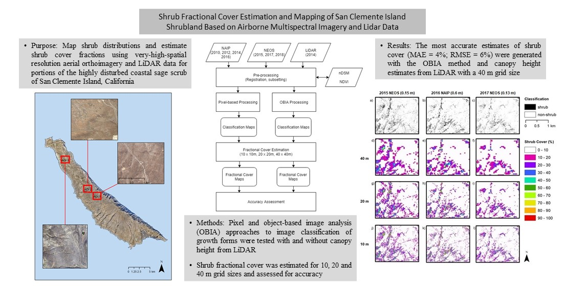
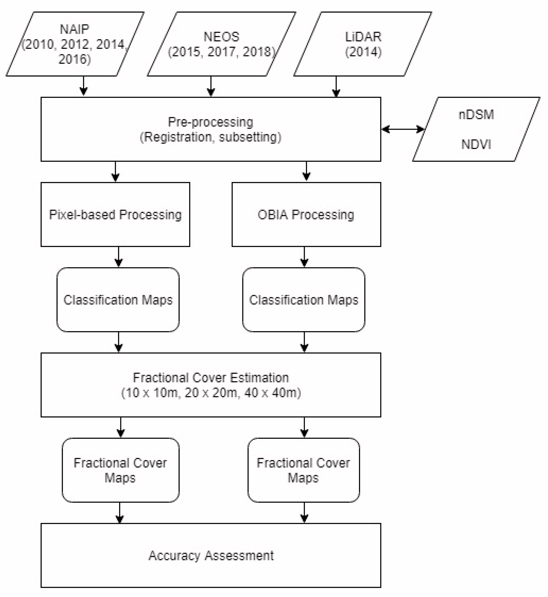
The primary objective of this study is to test the accuracy of estimating and mapping shrub cover fractions across SCI based on the classification of several very-high-spatial-resolution multispectral orthoimagery types (mosaics of orthorectified imagery) and light detection and ranging (LiDAR) data. The aerial orthoimagery data sets were obtained from the United States National Agricultural Imagery Program (NAIP) and from a commercial provider, Near Earth Observation System, Ltd. (NEOS). An emphasis was placed on object-based image analysis approaches. An analysis of multi-temporal aerial orthoimagery data sets captured cover over a nine-year period (2010-2018) was conducted in the context of mapping shrub cover.

Object-based image analysis (OBIA) approaches have proven to be useful for the classification and mapping of shrubs [9,11,12]. Hamada et al. [9] and Laliberte et al. [11] found that OBIA routines tend to yield higher accuracy map products than other processing methods, including per-pixel classifiers and spectral mixture models. Hamada et al. [9] assessed both high- and low-resolution processing methods to generate growth form maps in a CSS community. The results showed that OBIA yielded lower error than pixel-based classification approaches based on maximum likelihood and artificial neural network routines, and spectral mixture analysis applied to high and moderate spatial resolution satellite data. Laliberte et al. [11] utilized a similar OBIA process for mapping growth forms in rangelands and further broke down the classification to the species level for shrubs and grasses. Species-level classifications were attained for the dominant shrub species, while grasses were especially difficult to separate by species [9,11].

Another advantage of OBIA is the ability for cost-effective long-term ecological monitoring of CSS communities. Stow et al. [13] demonstrated that OBIA methods are more appropriate for monitoring shrub cover changes than pixel-based methods, when applied to high-spatial-resolution and multi-temporal image datasets. Through multi-temporal analyses, life form cover changes can be tracked over time. Laliberte et al. [11] also highlights the advantage of more efficient remote sensing methods over ground-based measurements. However, there is a trade-off between the accuracy and computational cost of OBIA methods [14]. OBIA is semi-automated; therefore, it is often highly dependent on expert knowledge and user input for the development of the segmentation and classification scheme. However, machine learning is also a method that shows a lot of promise and researchers are increasingly using machine learning techniques for image classification. Machine learning may allow for more accurate feature extraction and classification of National Agricultural Imagery Program (NAIP) imagery. However, machine learning algorithms require a large amount of very accurately labeled training inputs [15], which typically involves some form of semi-automatic classification and subsequent manual digitizing for accurate label generation. Extensive field sampling is challenging to conduct for places such as San Clemente Island that has restricted access.

Hamada et al. [5,7] utilized 25 × 25 m and 50 × 50 m grids for fractional cover estimation. Spatial sampling units 25 × 25 m in size proved to be more appropriate for estimating fractional cover within CSS communities for comparative reasons, while a 50 × 50 m sampling unit is appropriate for estimating growth form cover from a management perspective. These plot sizes are the most common sampling units used for studying CSS communities and the maximum area used by resource managers for restoration efforts such as eradicating invasive plants and planting native species [5]. However, different size sampling units may be more appropriate for the heavily disturbed and recovering state of shrublands on SCI.

Based on the above, we address the following research questions in this study:

• Which data inputs and image processing approaches generate the most accurate shrub fractional cover maps?
• How does the incorporation of nDSM data, that enables quantification of shrub and tree canopy heights, affect the accuracy of the map products?
• Does an OBIA approach yield more reliable shrub cover estimates than a pixel-based approach when applied to NAIP (0.6 to 1 m spatial resolution) orthoimage datasets that are readily available for SCI since at least 2010?
• What is the most appropriate grid size for quantifying shrub cover fractions in the context of potential future monitoring, given the relatively disturbed nature of shrublands on SCI?

2. Study Area

SCI is the southernmost of the Channel Islands off the southern California coast. The island trends 34 km northwest to southeast and ranges from 2 to 7 km wide, and has the highest level of endemism of the Channel Islands with 47 species endemic to the island group and 17 species endemic to SCI. Six of these species are classified as endangered or threatened and have faced difficulties re-establishing due to anthropogenic disturbances [8].

Vegetation on SCI is composed of two major community types: grasslands and CSS. There are 382 plant species present, 272 of which are native [8]. SCI has the highest plant endemism of the Channel Islands with 47 species endemic to the island group and 17 to SCI [16]. The upland terrain on the central and eastern portions of the island are dominated by non-native annual grasses such as Avena ssp. (wild oats) and Bromus ssp. (bromes) [17]. The coastal sage scrub found on the low-elevation areas is categorized as maritime succulent scrub, including Opuntia littoralis (prickly pear cactus), Cylindropuntia prolifera (cholla), Lycium californicum (box thorn), and other drought-resistant species. Although they once had a wider distribution, CSS habitats and trees are now confined to the moist environments of the canyons due to historic overgrazing [17,18].

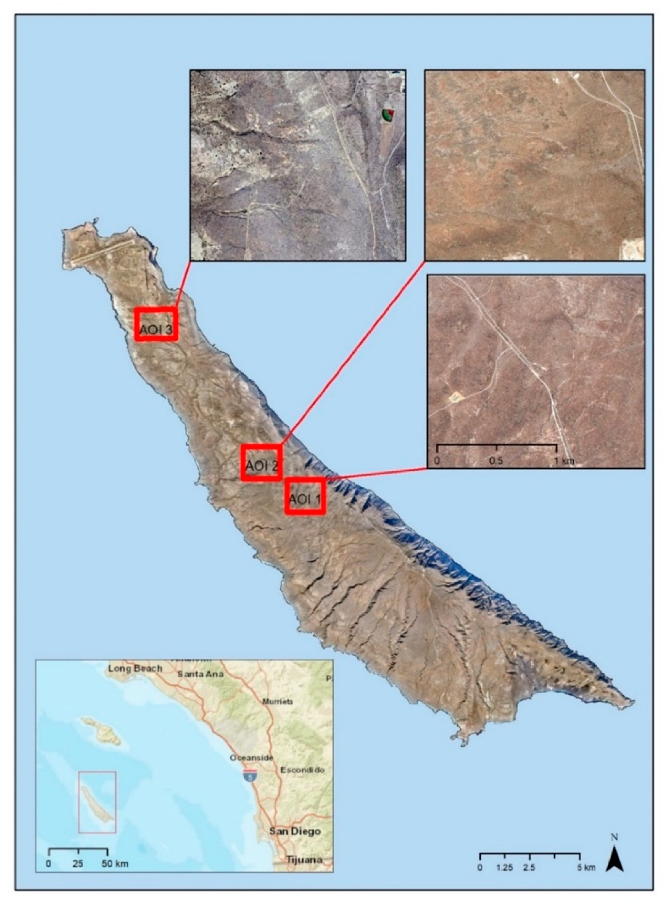
CSS at the lower elevations of the island tends to be found on isolated coastal bluffs and marine terraces. Vegetation is characterized by shrub and succulent species, including L. californicum, Rhus integrifolia, O. littoralis and C. prolifera (Figure 1). L. californicum is a low growing shrub found primarily on the lower terraces of the western shore. O. littoralis is prevalent on the terrace faces, which has served as shelter for shrub seedlings from herbivores. C. prolifera is found on the slopes of the southern end of the island [8].

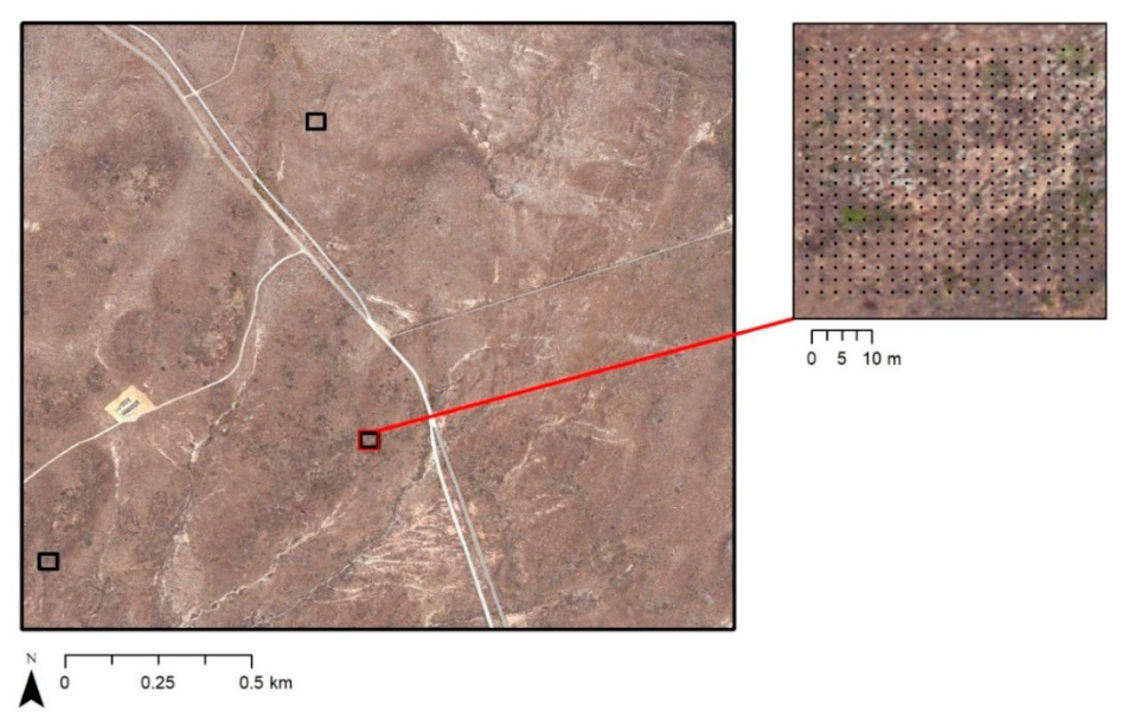
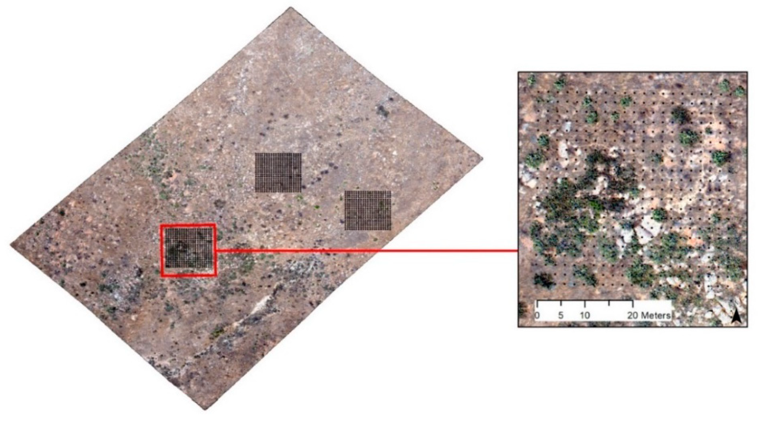
This shrub mapping research is focused on two general study areas on the island called Stone and Flasher. Two areas of interest (AOIs) were selected within the Stone study area on the eastern side of the island (Figure 1). These AOIs were selected based on the relative diversity of vegetation types, as well as the accessibility for performing ground-based accuracy assessments. A third AOI was selected within the Flasher study area located on the northwestern part of SCI to represent a range of shrub cover and diversity of shrub species not represented within the Stone study area.

AOIs 1 and 2 within the Stone study area are dominated by grasslands and a high cover of O. littoralis. The soil on the eastern slopes is composed of loam. AOI 3 in the Flasher study area is located the sand dunes on the northwestern coast. This area contains higher cover of L. californicum and R. intergrifolia. Soil in the Flasher study area is composed of a sandy loam with sand dunes on the coastline [8].

The island vegetation experienced severe degradation due to overgrazing and mechanical disturbances by feral goats, sheep and cattle. Sheep and cattle ranching ended in 1934, though feral herbivores were not completely eradicated until the early 1990s. The U.S. Navy has owned and operated on SCI since 1934. While disturbances to the island have been widespread, most of recent military-related disturbances have occurred in the southern third of the island. Since 1996, half of the fires occurring on the island have occurred within the Shore Bombardment Area (SHOBA). However, these fires account for approximately 90% of the total acreage burned [8].

SCI has a Mediterranean-type climate which is characterized by cool, wet winters and hot, dry summers. On average, 95% of rainfall occurs between November and April, with the most occurring in January and February. June, July and August are the driest months with only 1% of the annual mean rainfall. Regional rainfall patterns are highly variable and unpredictable. Multi-year droughts punctuated by wet years are not uncommon [19].

Both precipitation and the time of year have an impact on the spectral and physical properties of vegetation. Seasonal changes in leaf color and leaf area index can show inconsistent vegetation cover when comparing imagery captured during different seasons. Sims et al. [20] found that a greater decline in normalized difference vegetation index (NDVI) than canopy chlorophyll index (CCI) during extreme drought, suggesting that canopy structure is affected more than leaf greenness.

Table 1. Monthly precipitation (mm) prior to imagery collection.

	NAIP 2010	NAIP 2012	NAIP 2014	NEOS 2015	NAIP 2016	NEOS 2017	NEOS 2018
Month of Collection	May	April	July	November	July	August	November
1 month prior	45.22	24.64	0.00	10.92	0.00	0.00	14.48
3 months prior	120.40	65.02	13.46	42.67	25.15	23.88	14.99
6 months prior	267.21	177.80	71.63	147.83	127.25	120.40	18.03

NAIP—National Agricultural Imagery Program. NEOS—Near Earth Observation System, Ltd.

shows the total precipitation for one, three and six months prior to the collection of aerial imagery used in this study [8,21,22]. The amount of precipitation leading into the growing season influences the greenness of different vegetation types and therefore the ability to discriminate and accurately classify them.

3. Materials and Methods

3.1. Data

Data utilized for the classification of shrubs include high-spatial-resolution aerial orthoimagery, a spectral vegetation index derived from such imagery, as well as shrub height information from a LiDAR-derived digital surface model, as shown in

Table 2. Data characteristics. Image datasets were obtained for both study areas with the exception of the Near Earth Observation System, Ltd. (NEOS) 2017 dataset, which was acquired only for the Stone study area.

Image	Date	Format	Spatial Resolution
NAIP 2010	May 2010	4-band RGB, NIR	1 m
NAIP 2012	April 2012	4-band RGB, NIR	1 m
NAIP 2014	July 2014	4-band RGB, NIR	1 m
NEOS 2015	November 2015	4-band RGB, NIR	0.15 m
NAIP 2016	July 2016	4-band RGB, NIR	0.6 m
NEOS 2017	August 2017	4-band RGB, NIR	0.13 m
NEOS 2018	November 2018	4-band RGB, NIR	0.08 and 0.15 m
nDSM 2014	September 2014	nDSM	0.5 m

NAIP—National Agricultural Imagery Program; NEOS—Near-Earth Observation Systems, Ltd.; RGB—Red, Green, Blue; NIR—Near Infrared; nDSM—normalized digital surface model.

.

Visible and near-infrared (NIR) orthoimagery produced by the NAIP and from a commercial aerial service provider were used to classify shrub and non-shrub growth forms and estimate fractional cover of shrubs within all three AOIs. Freely available NAIP orthoimages for 2010, 2102 and 2014 with 1 m ground sampling distance (GSD) and 2016 with 0.6 m GSD were obtained from U.S. Geological Survey web portals. In addition, we commissioned Near-Earth Observation System (NEOS), Ltd. to conduct aerial image acquisition of SCI. Digital four-band imagery was collected in November 2015, August 2017 and November 2018 with 0.15 m GSD. The 2015 NEOS imagery was captured using a dual camera imaging system, consisting of two Canon Mark II 5D Digital SLR cameras (21 megapixel), with one camera capturing imagery in the visible spectrum and one capturing NIR imagery. The 2017 and 2018 imagery collection by NEOS used two Nikon D810, 36-megapixel cameras. Image frames were collected with 80% forward and 70% sideways overlap to enable the generation of digital surface model (DSM) and orthoimages (see the Pre-Processing section below). Spaced individual frames were captured along a few flight lines with a nominal spatial resolution of 0.08 m were collected in 2017 for the Stone study area and in 2018 for both the Stone and Flasher study areas for accuracy assessment purposes.

NDVI layers were generated using red and NIR waveband digital number values for each image date for both NAIP and NEOS datasets and incorporated as an additional input feature for image classifications. NDVI was utilized as one of the inputs for image classification for the OBIA approaches. NDVI quantifies vegetation abundance by subtracting the red reflectance values from the NIR and then dividing by the sum of the NIR and red bands. The resultant values can potentially range between −1 and 1 (typically −0.2 to 0.7 in the study area), with healthy vegetation having relatively high leaf area indices on the higher, positive end of the NDVI gradient [23].

A DSM layer was used to assess the utility of normalized digital surface model (nDSM) data in the identification and classification of shrubs. In September 2014, LiDAR data were collected by Scripps Institution of Oceanography (SIO). LiDAR point cloud processing, rasterization, and differencing were conducted with Esri ArcMap 10.4.1 software. The average pulse density of the original lidar collection is 17 pulses per sq meter with vertical accuracy of 10 cm. A DSM and a bare ground digital elevation model (DEM) with 0.5 m spatial resolution were produced for the study areas. The resultant LiDAR derivative products were used to create the nDSM by raster differencing, such that the DEM was subtracted from the DSM [24]. The nDSM data provide information on shrub heights, including the upper leaves and branches of the canopy.

3.2. Methods

Methods for this study include image pre-processing, image segmentation, image classification, grid-based fractional cover estimation and accuracy assessment (Figure 2). Software utilized for image processing and analysis includes ERDAS IMAGINE, eCognition, and ArcMap.

3.2.1. Pre-Processing

NEOS red, green, and blue (RGB) color images and NIR images were subject to photogrammetric processing to generate georeferenced orthoimages for the Stone and Flasher study areas. Three-band RGB images were co-registered to NIR bands to create four-band images. These images were subject to digital surface modeling, georeferencing, orthorectification and mosaicking operations imagery using Agisoft Photoscan software.

All orthoimagery datasets were projected to the WGS 1984 UTM 11N coordinate system and co-registration between images was refined using AutoSync Workstation in ERDAS IMAGINE. AutoSync Workstation uses automatic tie point collection as control for image-to-image warping transformations. Following this co-alignment processing, co-registration errors for the seven orthoimages were <1.5 m.

3.2.2. Pixel-Based Classification

Pixel-based classification was conducted on the 2010, 2012, 2014 and 2016 NAIP images using a supervised maximum likelihood classifier and signature creator tool in ERDAS IMAGINE. To ensure that classification products were as consistent and stable as possible, pixels corresponding to the same training areas were used for classification of each image dataset. Training samples were selected for each of the three growth form types (shrub, herb and bare/developed), with separate samples for grass and forb subtypes of the herb class. Each growth form type was broken into multiple sub-classes to account for intra-class spectral variability due to soil background and species composition. Sub-classes that represented a common cover type were kept independent in the classification process. Maps were exported and sub-classes were then combined to form their parent growth form class. Further grouping yielded classification maps portraying shrub and non-shrub distributions.

3.2.3. Object-Based Image Analysis

Trimble’s eCognition software was used to implement the OBIA classification approach. Rulesets, the user-defined processes which control image segmentation and classification, were established through trial and error. Multiresolution image segmentation, which locally minimizes the image brightness heterogeneity was used to generate image objects. Segmentation parameters include scale (local heterogeneity), color (spectral information) and shape (compactness and smoothness). Lower scale parameter values were selected for the NAIP datasets with a 0.6 m spatial resolution (2016), than the NEOS 2015 and 2017 datasets that have a finer spatial resolution. Optimal segmentation scales were based on parameter values that yielded segments having greater internal homogeneity and variability with neighboring segments [25]. Parameters were fine-tuned for each dataset in an attempt to ensure consistency in the segmentation processes. OBIA was not tested for the NAIP imagery from 2010 to 2014 due to the coarser (1 m) resolution. OBIA is an effective approach for high-spatial-resolution imagery, while pixel-based is more appropriate where patches or individual plants have characteristic dimensions near the ground sampling distance associated with a pixel.

After segmentation, image objects were classified according to growth form types, based on object features (inputs) utilized in the rulesets. The image classification rules were based on the mean values for the RGB and NIR layers, as well as the NDVI, brightness (average digital number of RGB bands) and max difference (maximum difference between mean values of RGB bands) values. To ensure consistent classification, the same ruleset was used for each image dataset, with different thresholds levels for each feature input. Each ruleset was modified to account for spectral-radiometric variation between the dates. This variation may be due to differences in the time of day and year that the imagery was captured, as well as sensor radiometry.

To assess the utility of nDSM data for the classification of shrubs, separate rulesets were developed to include the nDSM values. The nDSM data for this study are only available for 2014, so classification using nDSM information was assessed for the higher resolution NEOS 2015, NAIP 2016, NEOS 2017 and NEOS 2018 datasets. The resultant maps were compared to the OBIA derived maps without the nDSM incorporated.

The process flow outlining the segmentation and classification scheme and rulesets is illustrated in Figure 3. Segmented objects were first classified based on the growth form (shrub, forb, grass, tree or other non-vegetation cover). Higher-spatial-resolution image datasets were further classified to distinguish shrub species for objects classified as shrub growth form type. After the classification process, the resultant maps were exported to ERDAS IMAGINE Image (.img) file format.

3.2.4. Fractional Cover Estimation

Growth form classification maps generated from each of the orthoimages were imported into ArcMap for fractional cover estimation and mapping. Soil, rocks, bare, and non-shrub vegetation were combined to form a single, non-shrub class, while the shrubs retained as the class of primary interest.

A grid overlay was created using the Fishnet tool in ArcMap. Shrub cover was estimated for three different grid cell sizes, 10 × 10 m, 20 × 20 m and 40 × 40 m cells. While the 25 × 25 m and 50 × 50 m grid sizes are the standard sizes for quantifying fractional cover of growth forms, smaller and nested grid cell sizes were assessed to determine which grid size provides greatest accuracy of shrub cover estimation and most sensitive to the relatively low shrub cover fractions occurring on SCI [5,7]. Shrub cover was calculated for each grid cell using the Tabulate Area tool. Fractional cover maps portray the percentage of shrub cover within each grid cell using equal interval classes with 10% increments, though quantitative shrub cover estimates were retained at the 40 m level.

3.2.5. Accuracy Assessment

Gridded shrub cover estimates derived from different input data and image analysis approaches were assessed for accuracy based on reference data generated from a combination of field sampling and interpretation of ultra-high-spatial-resolution imagery. The 0.08 m resolution imagery and field sampling were used as reference data for the accuracy assessment. A total of 37 grids were assessed, seven through field sampling and observations, and 30 through sampling and interpretation of true color and false color infrared displays of 0.08 m orthoimages. The accuracy assessment grids were randomly located within the domains of the fractional cover maps.

Field sampling took place in September of 2019. Of the seven field sampling grids, three were located in AOI 1 and two within AOI 2 and in AOI 3. Figure 4 provides an example of the sample plot distribution and sampling grid for AOI 1. The field sampling grids are 40 × 40 m containing grid points with x and y spacing of 2 m. In the field, an interpreter navigated to the corners of each plot using Global Positioning System (GPS) data. A meter tape was used to locate grid point locations at 2 m intervals. At each point, a biologist determined the growth form type (shrub, herb or bare). If a shrub was present, the shrub species was identified. For the 10 × 10 m grid, 25 points per grid cell (5 × 5 points) were used in the calculation of shrub cover. For the 20 × 20 m grid, 100 points per grid cell (10 × 10 points) used. This was done to avoid having the overlapping points used for the calculation of two neighboring cells. The very top row and right column of points were not used in the calculations. For the 40 × 40 m cover calculation, all the points were used. This led to small differences in the estimates when averaging the smaller grids up to the larger 40 m grid.

Thirty additional 40 m × 40 m plots (10 per AOI) were sampled, by visual image interpretation at grid points spaced 2 m (in x and y) apart. The grids were randomly located on the ultra-high-spatial-resolution (0.08 m) NEOS orthoimagery (Figure 5) collected in 2017 and 2018. An independent interpreter interpreted and coded the growth form type at each grid intersection location and when shrub was present, recorded the shrub species. The image interpreter was also one of the biologists involved in the field sampling but was not involved in the automated image classification process. Shrub cover was quantified for 10 m × 10 m, 20 m × 20 m, and 40 m × 40 m grid sizes, as per the field-estimated plots. Five additional grids were sampled through both sampling methods for a comparison of field sampling and image interpretation shrub cover values.

4. Results

4.1. Image Classification

Image classification was implemented using pixel- and object-based methods to create maps of growth form classes (shrub and herb), as well as non-vegetation land cover (bare ground/soil or developed). Shrub/non-shrub maps were derived from growth form maps that were generated with spectral feature inputs to two image classification approaches, pixel-based (Figure 6a) and OBIA (Figure 7a), as well as by OBIA with nDSM included with spectral feature inputs (Figure 8a). Varying inputs and classification procedures resulted in maps portraying different shrub cover patterns. These maps provided the basis for estimating and mapping shrub fraction at several grid scales.

When comparing the classification products derived from multiple dates of 1 m NAIP imagery, the pixel-based shrub maps portray a decrease in shrub cover from 2010 to 2016. However, this apparent drastic loss of shrub cover is associated with misclassification of shrub growth forms, specifically an over-classification of shrubs in the lower spatial resolution NAIP imagery that was available for the earlier (2010–2014) period.

The OBIA classifier with nDSM and imagery inputs used the same classification rule sets as the OBIA method with only image inputs, other than the addition of nDSM thresholds in the ruleset. The addition of the nDSM data was critical for differentiating shrubs from other green vegetation.

4.2. Fractional Cover Maps

Maps indicating shrub fractional cover were generated using the shrub/non-shrub maps that were derived from each classification method and input combination. Shrub fractional cover maps for AOI 1 are shown in Figure 6 (pixel-based), Figure 7 (OBIA w/o nDSM) and Figure 8 (OBIA w/ nDSM). These maps are displayed as 10 percent intervals of fractional cover at the three grid sizes.

4.3. Accuracy Assessment

4.3.1. AOI 1 and 2

Root mean square error (RMSE) and mean absolute error (MAE) estimates for the fractional cover products from the three classification approaches for AOI 1, AOI 2 and both AOI combined are listed in

Table 3. Root mean square error (RMSE) and mean absolute error (MAE) values for the fractional cover products of AOI 1.

	40 m		20 m		10 m
Product	RMSE	MAE	RMSE	MAE	RMSE	MAE
NAIP May 2010 pixel	10.36	7.73	13.53	9.18	18.95	12.42
NAIP April 2012 pixel	15.64	11.59	21.21	14.97	23.14	15.86
NAIP July 2014 pixel	14.75	10.33	15.83	11.11	18.22	12.12
NAIP July 2016 pixel	10.14	7.25	11.43	7.92	13.81	9.30
NEOS November 2015 OBIA	8.71	5.76	10.53	7.01	14.31	9.11
NAIP July 2016 OBIA	6.27	5.11	9.31	5.91	12.96	8.04
NEOS August 2017 OBIA	10.97	7.85	12.76	8.68	15.43	10.30
NEOS November 2015 OBIA w/ nDSM	6.37	3.95	8.45	5.83	12.55	8.01
NAIP July 2016 OBIA w/ nDSM	7.56	5.80	10.02	6.94	13.81	9.30
NEOS August 2017 OBIA w/ nDSM	7.91	5.59	9.93	6.67	13.32	8.57

,

Table 4. Root mean square error (RMSE) and mean absolute error (MAE) values for the fractional cover products of AOI 2.

	40 m		20 m		10 m
Product	RMSE	MAE	RMSE	MAE	RMSE	MAE
NAIP May 2010 pixel	15.63	11.89	19.91	13.52	23.46	15.65
NAIP April 2012 pixel	14.46	10.12	16.69	10.95	19.96	13.19
NAIP July 2014 pixel	11.52	10.14	12.64	10.53	15.09	11.63
NAIP July 2016 pixel	7.62	5.12	11.32	7.10	14.47	8.68
NEOS November 2015 OBIA	10.88	7.22	13.38	8.72	15.64	10.30
NAIP July 2016 OBIA	14.93	9.27	16.63	10.27	20.91	12.17
NEOS August 2017 OBIA	8.72	6.75	10.09	7.42	13.90	9.19
NEOS November 2015 OBIA w/ nDSM	8.74	5.01	11.85	7.29	14.21	8.82
NAIP July 2016 OBIA w/ nDSM	13.19	8.07	15.44	9.24	20.08	11.81
NEOS August 2017 OBIA w/ nDSM	9.63	6.74	11.03	6.77	13.06	8.24

and

Table 5. Combined Root mean square error (RMSE) and mean absolute error (MAE) values for the fractional cover products of AOI 1 and 2.

	40 m		20 m		10 m
Product	RMSE	MAE	RMSE	MAE	RMSE	MAE
NAIP May 2010 pixel	13.16	9.73	16.90	11.26	21.23	13.97
NAIP April 2012 pixel	15.08	10.88	19.17	13.04	21.67	14.58
NAIP July 2014 pixel	13.30	10.24	14.39	10.83	16.79	11.89
NAIP July 2016 pixel	9.02	6.23	11.38	7.53	14.13	9.00
NEOS November 2015 OBIA	9.81	6.46	11.99	7.84	14.96	9.68
NAIP July 2016 OBIA	11.29	7.11	13.34	8.00	17.24	10.02
NEOS August 2017 OBIA	9.96	7.32	11.56	8.08	14.72	9.77
NEOS November 2015 OBIA w/ nDSM	7.60	4.46	10.22	6.53	13.37	8.40
NAIP July 2016 OBIA w/ nDSM	10.64	6.89	12.91	8.04	17.11	10.50
NEOS August 2017 OBIA w/ nDSM	8.78	6.14	10.47	6.72	13.20	8.41

, respectively. Lower RMSE and MAE values were attained for the products based on the higher/finer spatial resolution imagery from 2015, 2016 and 2017. For AOIs 1 and 2 combined, the minimum MAE value is 4.46 for the 2015 OBIA with nDSM product at the 40 m grid level, meaning the difference between the mapped cover and reference data is 4.46% shrub cover (Table 5). For both AOIs, the lower spatial resolution NAIP images for 2010, 2012 and 2014 that were classified using a pixel-based method yielded the highest RMSE and MAE (i.e., greatest apparent error in fractional cover estimates), with RMSE values ranging from 13.16 to 15.08 and MAE values from 9.73 to 10.88 for the 40 m grid size.

The largest (40 m) grid yielded the most accurate shrub cover estimates, with the 10 m grid size maps having the highest estimated errors. The 2015 OBIA with nDSM approach yielded the highest accuracy at the 40 m level with an MAE of 4.46%, 6.53% at the 20 m grid level, and 8.40% at the 10 m level (Table 5).

Incorporating the nDSM as a feature input to OBIA yielded shrub cover estimates that agreed more closely with the reference data than the estimates from the product based only on the four-band imagery. Accuracies are higher for products incorporating the nDSM data for the 2016 NAIP imagery, as well as the 2015 and 2017 NEOS imagery. The 2015 and 2017 OBIA with nDSM yielded maps with higher accuracies than the OBIA method without nDSM at all grid size levels. The 2016 OBIA with nDSM product is more accurate than that produced through OBIA without nDSM method at all grid levels, though the accuracies are essentially the same at the 10 m grid level.

Combining the accuracy results for both AOIs 1 and 2, we see that the incorporation of the 2015 NEOS multispectral and nDSM data as input to OBIA yields the lowest error estimates for the shrub fractional cover maps. Using only NEOS multispectral image inputs, a regression of the mapped shrub cover on the reference shrub cover yields an R-square value of 0.60. With the nDSM data included, the R-square value is higher at 0.84 (Figure 9). In both cases, the image classification products tended to underestimate shrub cover relative to the reference data, as indicated by a best fit line that is shallower than the 1:1 line.

Inclusion of the nDSM in the OBIA classifier did not result in the same higher level of accuracy for the 2016 NAIP products, as for classifications using the higher spatial resolution images for 2015 and 2017. Moreover, the pixel-based method applied to the 2016 NAIP imagery yielded a shrub cover map with lower error than both OBIA methods. For the 2016 NAIP imagery, the pixel-based method yielded the highest R-squared value of 0.69, while the OBIA method yielded products with greater estimation errors with an R-squared of 0.63. The addition of the nDSM resulted in a higher accuracy for the OBIA method, yielding an R-squared value of 0.67 (Figure 10). While the scatter is substantial, the OBIA with nDSM line is close to the 1:1 line, with a slight underestimation of the cover for the image classification-based estimates.

4.3.2. AOI 3

To test how well the highest performing classification approaches worked for a different study area, we applied OBIA to the three highest spatial resolution image sets covering AOI 3; 2015 NEOS, 2016 NAIP and 2018 NEOS (that yielded the most accurate shrub cover maps). AOI 3 was selected as a test area within the Flasher portion of SCI because it contains relatively high cover of Lycium californicum and Rhus integrifolia shrubs, which either were not present or were sparsely present in limited areas of AOIs 1 and 2. The pixel-based method with the 2016 NAIP imagery was also tested to determine if it yielded more accurate shrub cover products than the OBIA with nDSM method for the 0.6 m resolution imagery, as was the case for AOIs 1 and 2. Shrub fractional cover maps with 10% increments for 10, 20 and 40 m grids are shown in Figure 11.

Comparing the 2015 and 2018 NEOS products, there is a large difference in shrub cover. Both images were collected in November, so the difference is likely due to the amount of precipitation for each year. In 2015, 147.83 mm of precipitation was recorded in the 6 months prior to imagery collection, while only 18.03 mm was recorded in the 6 months prior to imagery collection in 2018.

As for AOIs 1 and 2, the shrub cover products for AOI 3 created using the 2015 and 2017 imagery with the OBIA and nDSM method yielded shrub cover maps with the lowest RMSE and MAE values relative to the reference data. The most accurate map is the 2015 NEOS OBIA product with the 40 m grid yielding MAE values of 10.80 and a RMSE value of 13.99 (

Table 6. Root mean square error (RMSE) and mean absolute error (MAE) values for AOI 3 fractional cover products.

	40 m		20 m		10 m
Product	RMSE	MAE	RMSE	MAE	RMSE	MAE
2016 pixel	27.71	21.82	29.85	23.82	32.18	25.29
2015 OBIA w/ nDSM	13.99	10.80	18.65	13.98	23.22	17.74
2016 OBIA w/ nDSM	18.27	14.92	23.65	17.97	29.30	22.05
2018 OBIA w/ nDSM	15.63	11.55	18.30	13.79	22.09	17.59

). Unlike the results from the first two AOIs, the 2016 pixel-based method exhibited greater error than the OBIA with nDSM method. The 2016 pixel based fractional cover product has the highest MAE of 21.82, while the 2016 OBIA with nDSM product has an MAE of 14.92.

Shrub estimates for the AOI 3 products are less accurate than those for AOIs 1 and 2. This is most likely due to an under-classification of shrubs, particularly L. californicum. While the nDSM proved useful in differentiating shrubs from the predominant herbaceous cover of the study areas, it exhibits little to no height signal for L. californicum. This may be because the light pulses from the LiDAR sensor were not able to penetrate the very dense, low stature canopy typical of L. californicum on SCI [21].

Overall, the 2015 OBIA with nDSM product yielded the lowest RMSE and MAE values for all three AOIs. However, R-square values are similar (0.81) for the 2015 and 2017 products when comparing shrub cover estimates with reference data samples (Figure 12).

Five grids were sampled using both image interpretation and field sampling for a comparison of the two accuracy assessment methods. Three of the grids show close agreement, while two points had higher shrub cover in the field compared to the image interpretation results (

Table 7. Field sampling and image interpretation shrub cover value comparison.

Dominant Shrub Species	Field Shrub Cover (%)	Image Interpretation Shrub Cover (%)	Difference (%)
R. integrifolia	17.69	20.86	−3.17
O. littoralis	47.62	24.26	23.36
O. littoralis	60.77	32.43	28.34
O. littoralis	17.91	18.59	−0.68
L. californicum	65.31	69.16	−3.85

). Large differences between the field sampling and image interpretation values are likely due to challenges faced during field sampling. The two grids with large differences in shrub cover values were located in areas with high cover of O. littoralis. The field interpreters were not able to follow the 2 m grid points across some of the dense thickets of O. littoralis leading to an estimation of how much cover was actually present. The MAE between the two estimates is 11.88, meaning the average difference between the shrub cover estimated in the field and image interpretation is 11.88%.

5. Discussion

5.1. Seasonality

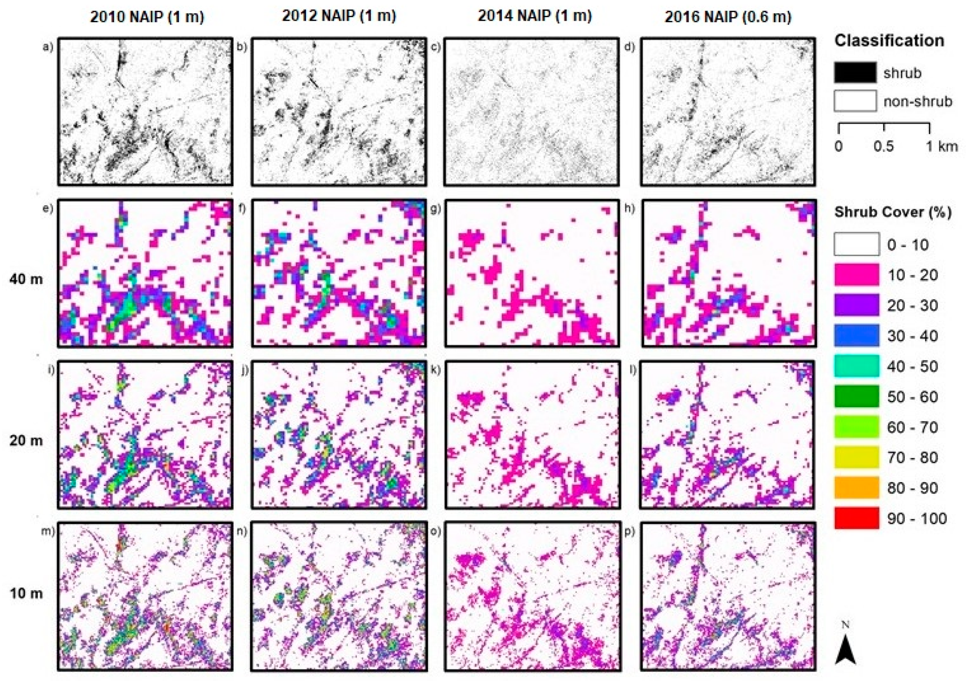
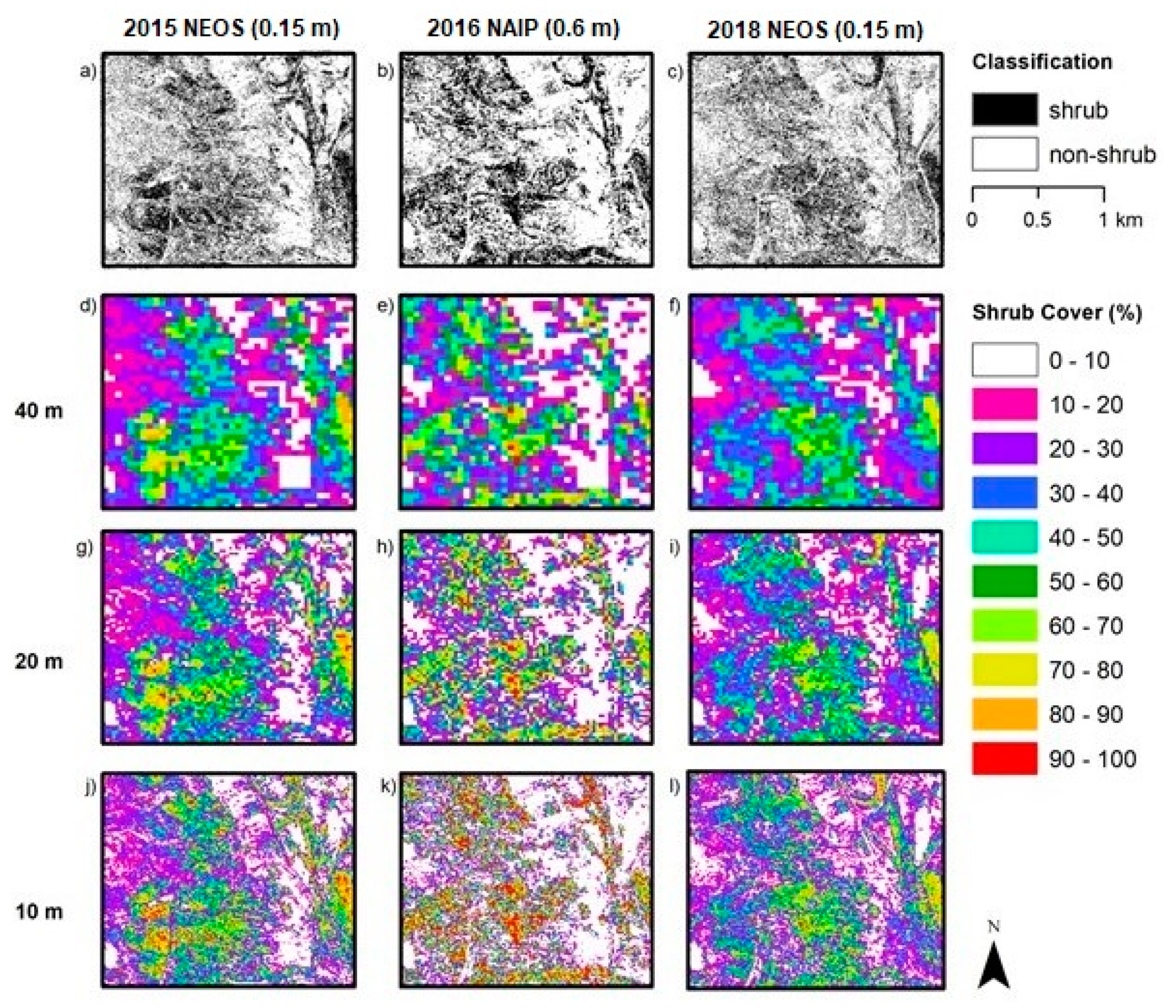
Aerial orthoimagery analyzed in this study was captured during different years and seasons, resulting in different vegetation conditions associated with vegetation phenology and available plant moisture. NAIP imagery for 2010, 2012, 2014 and 2016 were acquired in the spring and early summer, while the NEOS imagery for 2015, 2017 and 2018 were acquired in the late summer and fall. Seasonal variation in plant phenology causes differences in leaf and canopy properties between growth form types over the year and, therefore, differences in spectral reflectance signatures. During the spring growing season shrubs and herbs “green up” meaning increases in vigor, leaf area and canopy cover. As the season progresses into summer and fall, herbaceous plants senesce, while the shrubs maintain more green leaf cover. These differences in timing in image capture impact the procedures and rulesets for classifying vegetation.

Precipitation amounts for 2010 and 2012 were relatively high. Moreover, the study area receives greater precipitation during the December through March period (i.e., wet season) (Table 1). Since 2010 and 2012 experienced greater precipitation and the imagery was captured in spring, herbs were green longer (along with shrubs) and not senescent until later than normal, which likely led to the over-classification of shrub cover. The year 2014 was an especially dry (drought) year, which may have caused some die off of shrubs or reduction in vigor and green leaf cover. In addition, the 2014 NAIP imagery was captured in the summer, whereas the 2010 and 2012 images were captured in spring. Shrub cover maps for 2014 exhibited the lowest estimated shrub cover. The 2015 and 2017 NEOS imagery was collected in fall and late summer, respectively, when more of the herbaceous cover had senesced, such that shrubs and herbs exhibited substantial differences in spectral signatures.

5.2. Image Spatial Resolution

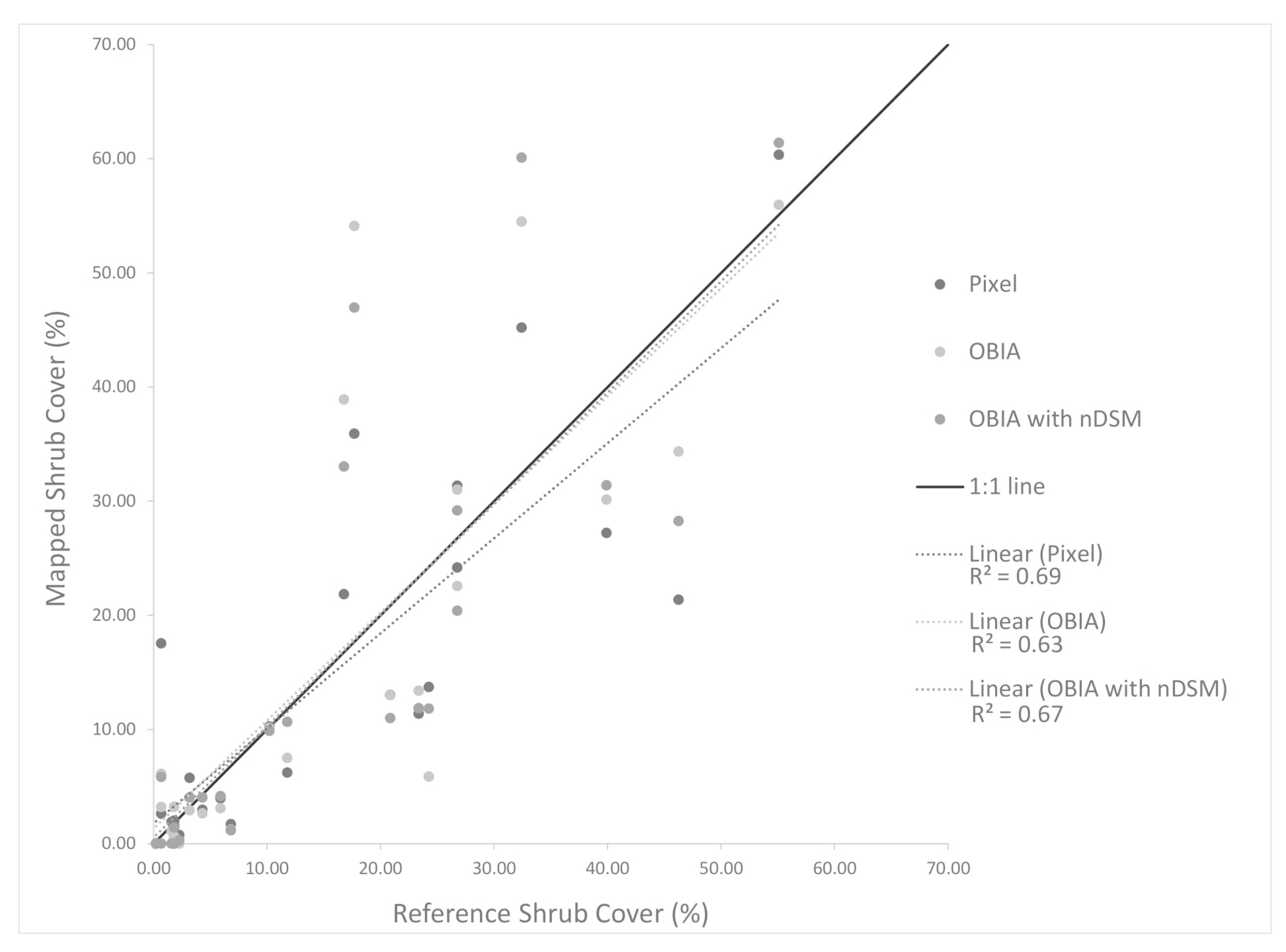
Image spatial resolution can also influence the choice of classification method chosen for mapping shrubs and the resultant accuracy of shrub cover estimates. The earlier NAIP imagery dates (2010, 2012 and 2014) have the lowest (coarsest) resolution of 1 m while that of the 2016 NAIP imagery is 0.6 m. The higher spatial resolution 2016 imagery yielded the highest accuracy shrub cover estimates of the NAIP images tested. The pixel-based approach applied to the 2016 NAIP imagery yielded more accurate estimates than for the OBIA approach for two of the three AOI, suggesting that a pixel-based approach may be a viable option for mapping shrub cover over time based on NAIP imagery. This may be useful for future applications of shrub tracking as NAIP now has set more consistent collection standards for summer image acquisitions with a 0.6 m spatial resolution.

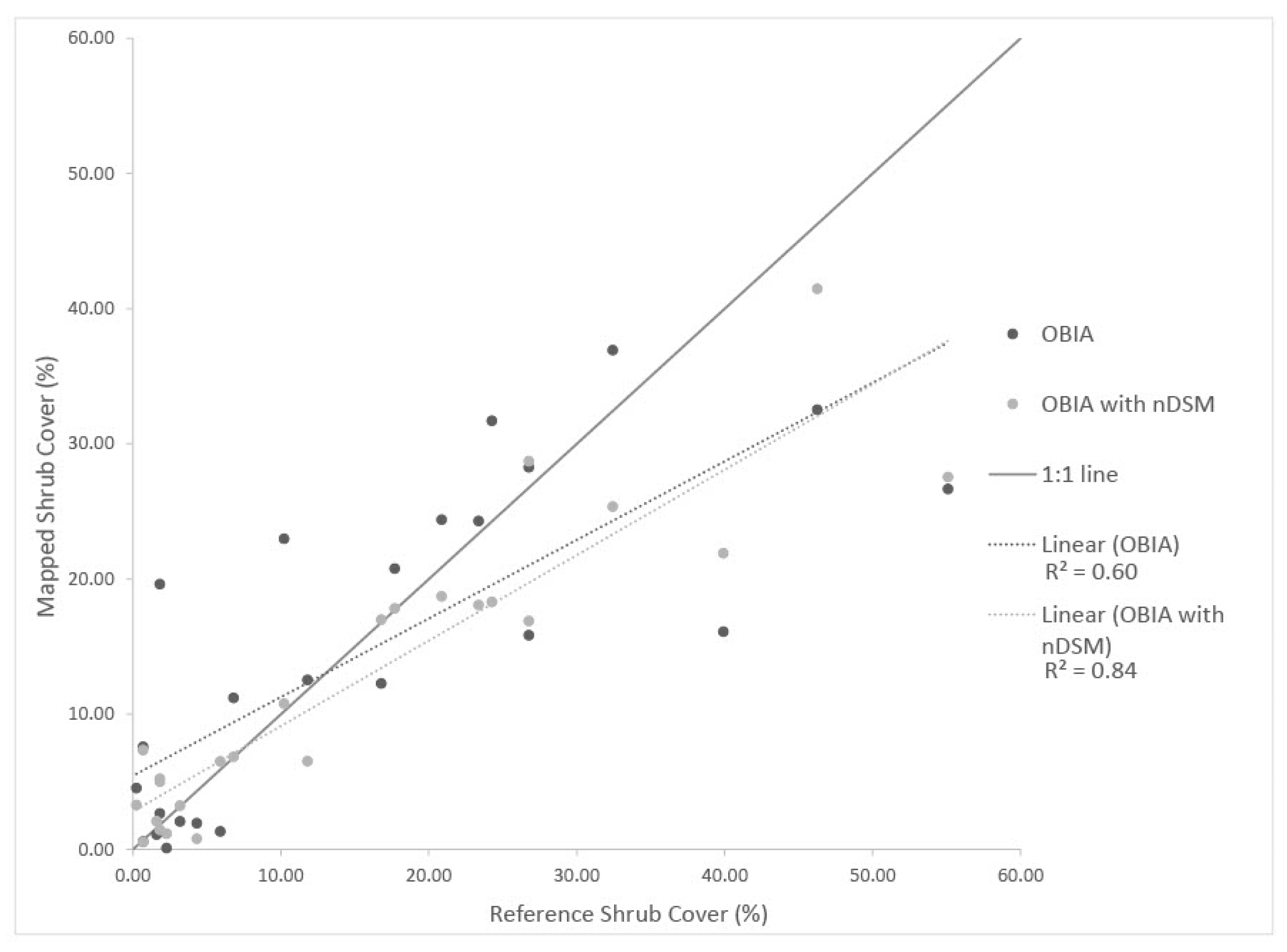
5.3. nDSM

The OBIA approach with the incorporation of nDSM allowed shrubs to be classified uniquely from the predominant non-native grasslands of San Clemente Island, based on shrub height information. With the addition of nDSM data, OBIA applied to NEOS imagery yielded the highest accuracy for mapping shrub cover. However, for AOI 3, the nDSM data were not as helpful for successfully classifying shrubs due to the lack of height signal from the predominant, low stature and densely packed shrub species, L. californicum. With minimal height information, classification was based primarily on multispectral brightness and NDVI feature inputs.

A single nDSM product, based on LiDAR data collected in 2014, was available for the study period. The single-time LiDAR-derived nDSM proved to be useful for the classification of shrubs. DSMs were generated from the highly overlapping NEOS multispectral imagery, as part of the Structure-from-Motion (SfM) processing in support of orthorectification of image frames. However, based on our cursory analyses, nDSM generated from SfM-derived DSM data were not sufficiently accurate or detailed to reliably classify shrubs vs. non-shrubs. Including a reliable nDSM derived from the same aerial image set as the orthoimage in the growth form classification process should allow changes in shrub height and expansion to be quantified, likely increasing the accuracy of shrub cover/change maps and estimates.

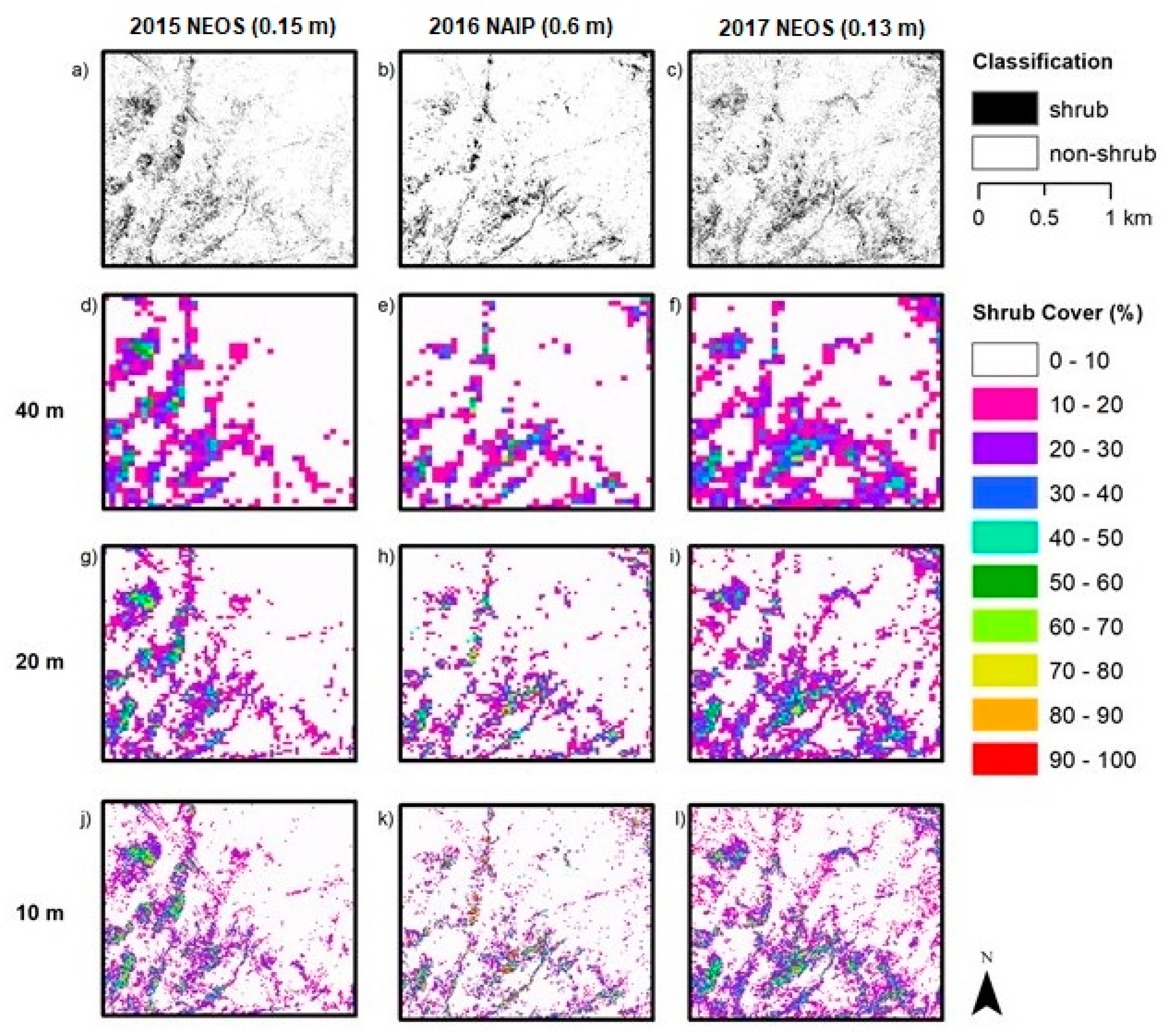
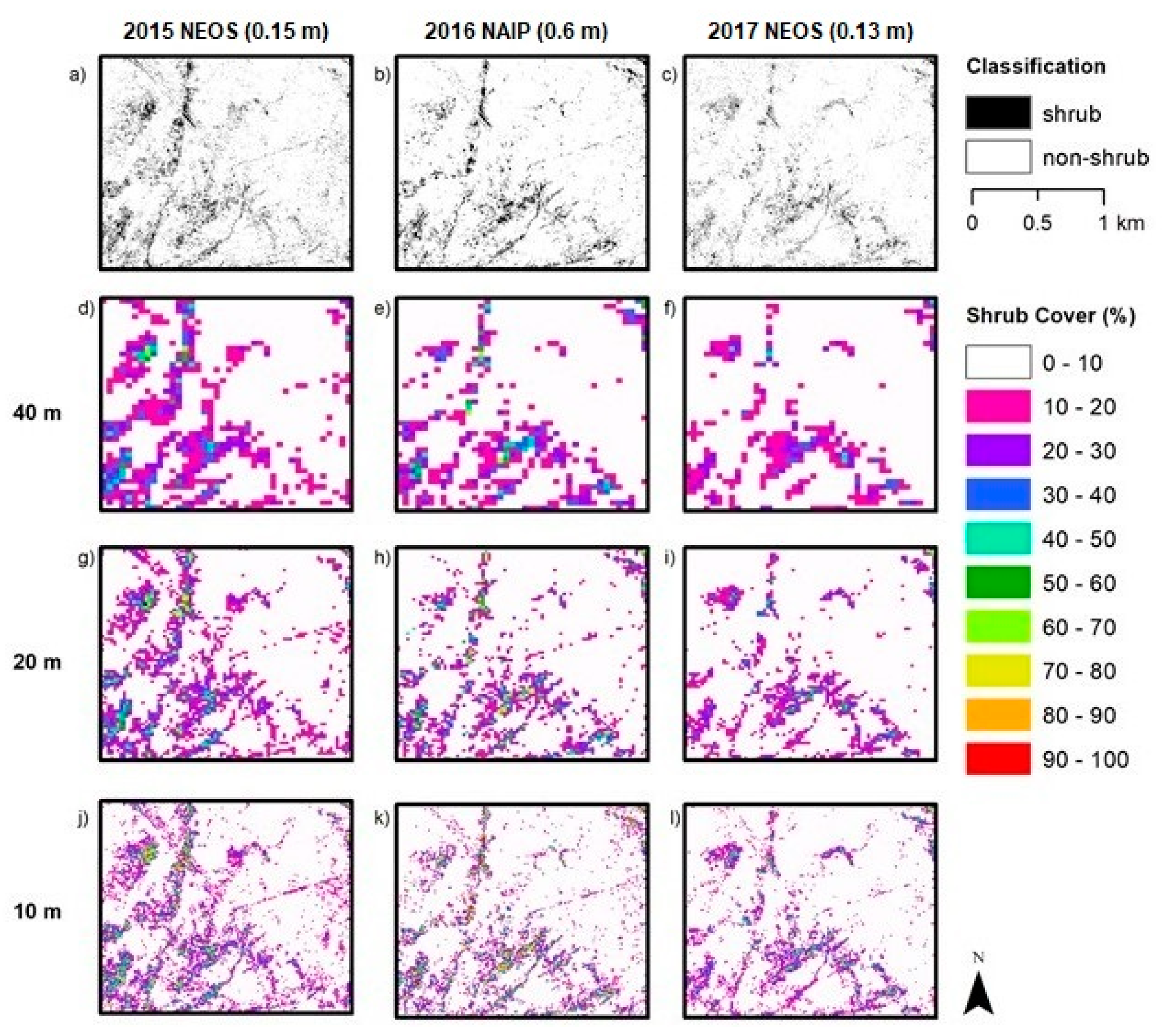
5.4. Fractional Cover Grid Size

Estimation of fractional vegetation cover is necessarily based on arbitrary sized and shaped spatial sampling units; for this study, square grids of three varying areal extents were tested. One criterion for determining the appropriate grid size for shrub monitoring is the sensitivity in capturing changes in shrub cover, which would tend to justify a smaller grid. For example, detection of a change in shrub cover within the 40 m grid would tend to require a greater amount of shrub cover change to yield a detectable signal, compared to the 10 m grid. However, the empirically based evidence from this study suggests that error and uncertainty in shrub cover estimates were least for the 40 m grid and greatest for the 10 m grid. A 20 m grid would seem to be a good compromise, as the error estimates for this level were only slightly greater than for the 40 m grid. Moreover, the 20 m grid is four times smaller for sensitivity purposes, and similar in size to the 25 m grid sampling scale that is advocated for monitoring growth form cover within CSS communities [1,7].

5.5. Challenges and Limitations

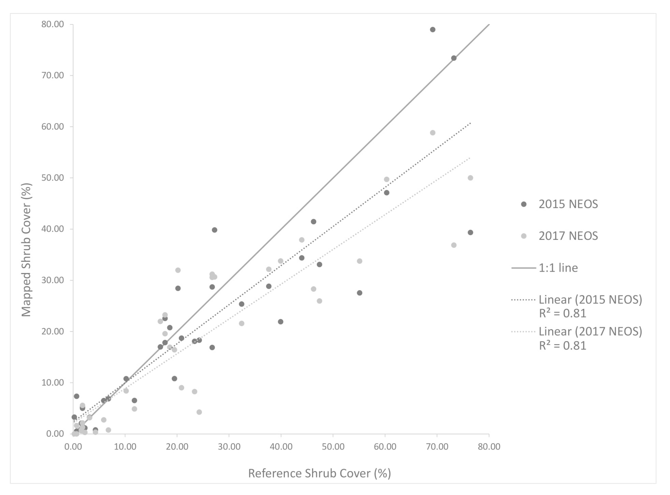
We found no sources of reference data on locations of shrubs for the earlier years (prior to 2015), and the reference data used in this study were only collected within a short period of time at the end of the study period. The reference data were generated by biologists conducting field sampling in September 2019 and through interpretation of aerial multispectral imagery captured in 2017 and 2018, having a spatial resolution twice as fine as that used for automated image classification. The 2015 and 2017 NEOS imagery resulted in more accurate classification products than the 2010 – 2016 NAIP products (Table 3, Table 4 and Table 5). These results are likely due to the higher resolution of the NEOS imagery but may also be related to the fact that the field- and image-based reference data were collected near the end of the study period. However, based on the assumption that little change has occurred in the eight-year period of this study and the lack of reference data from previous years, the reference data collected in 2019 provided the basis for accuracy assessment of all shrub cover products (i.e., for all years in the study period).

The coarser spatial resolution (1 m rather than 0.15 or 0.6 m) and lack of time-specific nDSM for the earlier years made the accurate classification and cover estimation of shrubs challenging. The 1 m resolution was too coarse to accurately resolve and identify some shrub, resulting in errors and uncertainty in representing shrub cover over space and time.

Shrub cover products generated with nDSM are clearly more accurate and reliable. However, changes in the cover and height of shrubs could render a single reliable nDSM as sub-optimal for tracking changes over time (as discussed above).

5.6. Recommendations for Future Research

While the goal of this study is to create a reliable shrub cover monitoring approach, the archived image data sets that are available are not sufficient to achieve this. However, this study allows us to make recommendations for follow-on research and future shrub cover monitoring programs. As mentioned in the previous section, consistent timing for imagery capture is important to image vegetation at a similar growth state each year. Imagery collected in the late summer or early fall is optimal for distinguishing green shrubs against a background of herbaceous cover that has senesced. The incorporation of canopy height information is also crucial for the classification of the relatively sparse, low-stature shrubs on San Clemente Island and other heavily disturbed shrublands. For this study, nDSMs representing vegetation heights were derived from airborne LiDAR data, which can be expensive. Another option is using DSM created through SfM. This method is cheaper; however, generating a high-quality nDSM from SfM can be challenging from slight motions of vegetation between capture of adjacent, overlapping image frames. Very accurate and precise ground control points and image capture during relatively still wind conditions are requirements for generating reliable DSMs from SfM procedures.

OBIA classification of very-high-spatial-resolution multispectral imagery appears to be the most appropriate image analysis approach for mapping shrub growth forms and estimating their fractional cover at SCI. This study has shown that an OBIA approach that incorporates high-spatial-resolution imagery and nDSM data yields higher accuracy shrub cover maps than pixel-based mapping. Using increasingly available DSM products in combination with temporally consistent, systematically acquired high-spatial-resolution imagery, mapping changes in shrub cover should be achievable in a reliable manner. This is the emphasis of our follow-on research.

6. Conclusions

Fractional cover analysis of shrubs can provide ecologically meaningful information for the conservation and restoration of CSS communities [7,10]. Fractional cover of shrubs is an indication of the integrity of shrubland ecosystems. Tracking changes in shrub cover over time from a baseline may provide a monitoring tool of CSS conditions and develop a trajectory for future recovery, as long as shrub cover maps are accurate and reliable.

The major factors that influenced the reliability of shrub mapping and fractional cover estimation include the date (time of year) the imagery was collected, the spatial resolution of the imagery, the type of classifier used, the inputs to the classifier, and the grid scale used for cover estimation. We tested both pixel-based and OBIA approaches for the classification of remotely sensed imagery. Upon comparing the shrub cover between 2010 and 2018, an apparent decrease in shrub cover is evident. However, it is likely that this apparent decrease is due to over-classification of shrubs in the earlier NAIP imagery.

This study was based on both readily available and newly acquired orthoimagery with varying spatial resolutions. We found that the higher spatial resolution datasets resulted in the most accurate shrub classification and cover estimation products. We also analyzed the utility of nDSM data for classifying shrubs with OBIA. The canopy height information contained within nDSM data yielded more accurate identification of shrub objects during the classification process than when based solely on the visible/NIR image brightness values. The object-based approach with nDSM input was found to be the most accurate for identifying shrubs in all but one case (2016 NAIP). The pixel-based classifications using the 2016 NAIP imagery performed nearly as well as the OBIA methods using nDSM for AOIs 1 and 2, which include shrub landscapes with 20–60% shrub cover. These landscapes should be the focus of future ecological monitoring as they are recovering from disturbance and may show varying degrees of shrub development or transition to herbaceous cover.

References

1. O’Leary, J.F.; Westman, W.E. Regional Disturbance Effects on Herb Succession Patterns in Coastal Sage Scrub. J. Biogeogr. 1988, 15, 775. [Google Scholar] [CrossRef]
2. Brennan, S.; Laris, P.S.; Rodrigue, C.M. Coyote Brush as Facilitator of Native California Plant Recovery in the Santa Monica Mountains. Madroño 2018, 65, 47–59. [Google Scholar] [CrossRef]
3. O’Leary, J. Californian coastal sage scrub: General characteristics and considerations for biological conservation. In Endangered Plant Communities of Southern California; Southern California Botanists, Rancho Santa Ana Botanic Gardens: Claremont, CA, USA, 1990; pp. 24–41. [Google Scholar]
4. Witztum, E.R.; Stow, D.A. Analysing direct impacts of recreation activity on coastal sage scrub habitat with very high resolution multi-spectral imagery. Int. J. Remote Sens. 2003, 25, 3477–3496. [Google Scholar] [CrossRef]
5. Hamada, Y.; Stow, D.A.; Roberts, D.A.; Franklin, J.; Kyriakidis, P.C. Assessing and monitoring semi-arid shrublands using object-based image analysis and multiple endmember spectral mixture analysis. Environ. Monit. Assess. 2012, 185, 3173–3190. [Google Scholar] [CrossRef] [PubMed]
6. Davis, F.; Stine, P.; Stoms, D. Distribution and Conservation Status of Coastal Sage Scrub in Southwestern California. J. Veg. Sci. 1994, 5, 743–756. [Google Scholar] [CrossRef]
7. Hamada, Y.; Stow, D.A.; Franklin, J. Quantifying Biological Integrity of California Sage Scrub Communities Using Plant Life-form Cover. J. Mediterr. Ecol. 2009, 10, 19–32. [Google Scholar]
8. Tierra Data Inc. Integrated Natural Resources Management Plan; Naval Auxiliary Landing Field: San Clemente Island, CA, USA, 2013. [Google Scholar]
9. Hamada, Y.; Stow, D.A.; Roberts, D.A. Estimating life-form cover fractions in California sage scrub communities using multispectral remote sensing. Remote Sens. Environ. 2011, 115, 3056–3068. [Google Scholar] [CrossRef]
10. Lippitt, C.L.; Stow, D.A.; Roberts, D.A.; Coulter, L.L. Multidate MESMA for monitoring vegetation growth forms in southern California shrublands. Int. J. Remote Sens. 2017, 39, 655–683. [Google Scholar] [CrossRef]
11. Laliberte, A.S.; Browning, D.M.; Herrick, J.E.; Gronemeyer, P. Hierarchical object-based classification of ultra-high-resolution digital mapping camera (DMC) imagery for rangeland mapping and assessment. J. Spat. Sci. 2010, 55, 101–115. [Google Scholar] [CrossRef]
12. Uyeda, K.A.; Warkentin, K.K.; Stow, D.A.; O’Leary, J.F.; Snavely, R.A.; Lambert, J.; Bolick, L.A.; O’Connor, K.; Munson, B.; Loerch, A.C. Vegetation mapping using hierarchical object-based image analysis applied to aerial imagery and lidar data. Appl. Veg. Sci. 2020, 23. [Google Scholar] [CrossRef]
13. Stow, D.; Hamada, Y.; Coulter, L.; Anguelova, Z. Monitoring shrubland habitat changes through object-based change identification with airborne multispectral imagery. Remote Sens. Environ. 2008, 112, 1051–1061. [Google Scholar] [CrossRef]
14. Freeman, M.P.; Stow, D.A.; Roberts, D.A. Object-based image mapping of conifer tree mortality in San Diego county based on multitemporal aerial ortho-imagery. Photogramm. Eng. Remote Sensing 2016, 82, 571–580. [Google Scholar] [CrossRef]
15. Maxwell, A.E.; Warner, T.A.; Vanderbilt, B.C.; Ramezan, C.A. Land cover classification and feature extraction from National Agriculture Imagery Program (NAIP) Orthoimagery: A review. Photogramm. Eng. Remote Sensing 2017, 83, 737–747. [Google Scholar] [CrossRef]
16. Wylie, D.D.J. Vegetation Change on San Clemente Island Following the Removal of feral Herbivores. Master’s Thesis, Montezuma Publishing, San Diego State University, San Diego, CA, USA, 2012. [Google Scholar]
17. Schoenherr, A.; Feldmeth, C.; Emerson, M. Natural History of the Islands of California; University of California Press: Oakland, CA, USA, 2003. [Google Scholar]
18. Rundel, P.W. Sage Scrub. In Terrestrial Vegetation of California; University of California: Berkeley, CA, USA, 2007; pp. 208–228. [Google Scholar]
19. U.S. National Park Service Channel Islands Weather. Available online: https://www.nps.gov/chis/learn/nature/weather.htm (accessed on 13 November 2018).
20. Sims, D.A.; Luo, H.; Hastings, S.; Oechel, W.C.; Rahman, A.F.; Gamon, J.A. Parallel adjustments in vegetation greenness and ecosystem CO2 exchange in response to drought in a Southern California chaparral ecosystem. Remote Sens. Environ. 2006, 103, 289–303. [Google Scholar] [CrossRef]
21. California State University Northridge San Clemente Island Climatic Monitoring Project. Available online: http://www.csun.edu/scisland/index.html (accessed on 10 February 2019).
22. Western Regional Climate Center RAWS USA Climate. Archive. Available online: https://wrcc.dri.edu/cgi-bin/rawMAIN.pl?caCNSC (accessed on 26 February 2019).
23. Jensen, J. Remote Sensing of Vegetation. In Remote Sensing of the Environment an Earth Resource Perspective; Pearson Prentice Hall Inc.: Upper Saddle River, NJ, USA, 2007; pp. 355–408. [Google Scholar]
24. Snavely, R.A.; Uyeda, K.A.; Stow, D.A.; O’Leary, J.F.; Lambert, J. Mapping vegetation community types in a highly disturbed landscape: Integrating hierarchical object-based image analysis with lidar-derived canopy height data. Int. J. Remote Sens. 2019, 40, 4384–4400. [Google Scholar] [CrossRef]
25. Ikokou, G.; Smit, J. A Technique for Optimal Selection of Segmentation Scale Parameters for Object-oriented Classification of Urban Scenes. S. Afr. J. Geomatics. 2013, 2, 358–369. [Google Scholar]
Figure 1. Overview map of San Clemente Island, California, with two areas of interest (AOIs) located in the Stone study area and a third AOI located in the Flasher study area.
Remotesensing 12 03608 g001
Figure 2. Data processing and analysis workflow.
Remotesensing 12 03608 g002
Figure 3. Object-based image analysis (OBIA) ruleset structure in eCognition.
Remotesensing 12 03608 g003
Figure 4. Distribution of field sampling grids for AOI 1 with field grid survey points shown in inset.
Remotesensing 12 03608 g004
Figure 5. Imagery used for image interpretation with sampling grid overlay.
Remotesensing 12 03608 g005
Figure 6. AOI 1 pixel-based classification for 2010, 2012, 2014 and 2016 across the top row (a–d), with the 40 m (eh), 20 m (i–l) and 10 m (m–p) fractional cover products in the rows below.
Remotesensing 12 03608 g006
Figure 7. AOI 1 object-based classification for 2015, 2016 and 2017 across the top row (a–c), with the 40 m (d–f), 20 m (gi) and 10 m (j–l) fractional cover products in the rows below.
Remotesensing 12 03608 g007
Figure 8. AOI 1 object-based classification with normalized digital surface model (nDSM) for 2015, 2016 and 2017 across the top row (a–c), with the 40 m (d–f), 20 m (gi) and 10 m (j–l) fractional cover products in the rows below.
Remotesensing 12 03608 g008
Figure 9. Comparison of 2015 NEOS products created using the OBIA with and without nDSM (40m grid) for AOI 1 and 2 combined.
Remotesensing 12 03608 g009
Figure 10. Comparison of 2016 NAIP fractional cover products for AOI 1 and 2, created using the pixel, OBIA and OBIA with nDSM methods.
Remotesensing 12 03608 g010
Figure 11. AOI 3 object-based classification products with nDSM for 2015, 2016 and 2017 (a–c), with the 40 m (d–f), 20 m (gi) and 10 m (j–l) fractional cover products below.
Remotesensing 12 03608 g011
Figure 12. Shrub cover values for AOI 1-3 compared to the reference shrub cover values for the OBIA with nDSM method using NEOS imagery. The 2015 and 2017 NEOS imagery classified using the OBIA with nDSM method yielded the highest R-square values.
Remotesensing 12 03608 g012