Improving Soil Thickness Estimations Based on Multiple Environmental Variables with Stacking Ensemble Methods


1
Key Laboratory of Watershed Geographic Sciences, Nanjing Institute of Geography and Limnology, Chinese Academy of Sciences, Nanjing 210008, China
2
School of Urban and Environmental Sciences, Huaiyin Normal University, Huai’an 223300, China
3
Institute of Crop Sciences, Chinese Academy of Agricultural Sciences/Key Laboratory of Crop Physiology and Ecology, Ministry of Agriculture, Beijing 100081, China
*
Author to whom correspondence should be addressed.
Remote Sens. 2020, 12(21), 3609; https://0-doi-org.brum.beds.ac.uk/10.3390/rs12213609
Submission received: 9 October 2020
/
Revised: 29 October 2020
/
Accepted: 30 October 2020
/
Published: 3 November 2020
(This article belongs to the Special Issue Remote Sensing for Biophysical and Biochemical Property of Crops and Natural Vegetation)
Abstract
:Spatially continuous soil thickness data at large scales are usually not readily available and are often difficult and expensive to acquire. Various machine learning algorithms have become very popular in digital soil mapping to predict and map the spatial distribution of soil properties. Identifying the controlling environmental variables of soil thickness and selecting suitable machine learning algorithms are vitally important in modeling. In this study, 11 quantitative and four qualitative environmental variables were selected to explore the main variables that affect soil thickness. Four commonly used machine learning algorithms (multiple linear regression (MLR), support vector regression (SVR), random forest (RF), and extreme gradient boosting (XGBoost) were evaluated as individual models to separately predict and obtain a soil thickness distribution map in Henan Province, China. In addition, the two stacking ensemble models using least absolute shrinkage and selection operator (LASSO) and generalized boosted regression model (GBM) were tested and applied to build the most reliable and accurate estimation model. The results showed that variable selection was a very important part of soil thickness modeling. Topographic wetness index (TWI), slope, elevation, land use and enhanced vegetation index (EVI) were the most influential environmental variables in soil thickness modeling. Comparative results showed that the XGBoost model outperformed the MLR, RF and SVR models. Importantly, the two stacking models achieved higher performance than the single model, especially when using GBM. In terms of accuracy, the proposed stacking method explained 64.0% of the variation for soil thickness. The results of our study provide useful alternative approaches for mapping soil thickness, with potential for use with other soil properties.
1. Introduction
Soil thickness is considered to play an important role in numerous areas, such as soil structure and function [1], vegetation growth [2], land surface energy flux [3], hydrology [4] and ecological land classification [5]. Traditional soil sampling is laborious, time consuming and difficult to carry out at large scales [6]. Currently, most modeling works require continuous and quantitative spatial soil information [7,8].
Digital soil mapping (DSM) techniques can be used not only to reduce sampling and analytical costs but also to obtain the spatial distributions of soil properties over large scales [9,10]. Current soil thickness mapping methods can be classified into three categories: (1) physically based models, (2) empirical-statistical based models built using environmental covariates, and (3) interpolation from point samples [11]. These mathematical or statistical methods are based on key landscape factors and processes that determine the formations of soil properties. Spatial patterns in soil thickness result from complex interactions of soil-forming environmental factors, including terrain relief, climate, parent material, biological factors, human activities, physical processes and time [6,12]. Quantitative environmental variables such as elevation, slope, aspect derived from digital elevation models and vegetation index derived from remote sensing data have been widely used. Qualitative environmental variables such as geomorphic maps, geological maps, land use types, and legacy soil maps could be important parameters for predicting soil properties [13,14].
Given the large numbers of environmental variables that characterize soil-forming factors from multiple aspects, the selection of appropriate variables is an important issue in DSM modeling [12]. The relationships between soil properties and environmental variables should be investigated to obtain reliable soil thickness estimations. It is commonly accepted that more detailed covariates could convey more spatial information, more adequately describe the interpretation of soil formation, and improve the accuracy of the soil property predictions [15,16,17]. However, some studies have shown that the use of all environmental variables would not necessarily improve the accuracy and cause the curse of dimensionality [18,19]. Some covariates may be useless, noisy, redundant and cause noise in modeling [20]. Variable selection should select the few most effective variables to reduce the spatial dimensions of the variables, simplify predictive models, improve accuracy, and provide robust models [21,22]. Therefore, it may be more effective to obtain fewer and more suitable variables to build a robust and simplified model for DSM.
Recently, various machine learning (ML) algorithms have become very popular in digital soil mapping, including: multiple linear regression (MLR) [23], regression trees (RT) [8], regression kriging (RK) [11,23], generalized additive model (GAM) [24], random forest (RF) [21], artificial neural networks (ANN) [25], and support vector regression (SVR) [26]. Early reviews on the strengths and weaknesses of these machine learning algorithms have been discussed in some published articles [6,27,28]. However, due to different working environments, some disputes still remain on which method is the best suited for DSM [25,29]. Therefore, machine learning algorithms should still be compared and evaluated under different landscapes in order to be able to make better judgements on which one is best suited for soil thickness [30].
Ensemble learning is a popular machine learning paradigm that integrates the predictions of individual single learners to achieve higher performance than that of a single learner [31]. Boosting, bagging and stacking are the three main ensemble methods [32]. The stacking approach can take advantage of the characteristics of different machine learning algorithms, reduce the variance of the single machine learning model, and provide better and more stable predictions. Previous studies have shown the potential of stacking models in improving the accuracy of soil property maps of soil organic carbon [33,34,35,36,37], soil total nitrogen [38], soil class [39], soil pH [40], and soil texture [41].
In this paper, we selected quantitative and qualitative environmental covariates and compare stacking ensemble approaches with four machine learning algorithms (MLR, SVR, RF, and extreme gradient boosting (XGBoost)) to create the optimal models and predict the soil thickness map in Henan Province, China. The specific objectives of this study were as follows: (1) to select optimal environmental variables for soil thickness estimation models; (2) to investigate the performance of the SVR, RF, and XGBoost models; (3) to evaluate the ability of stacking ensemble approaches to predict soil thickness; and (4) to draw spatial distribution maps of soil thickness for the study area.
2. Material and Methods
2.1. Study Area
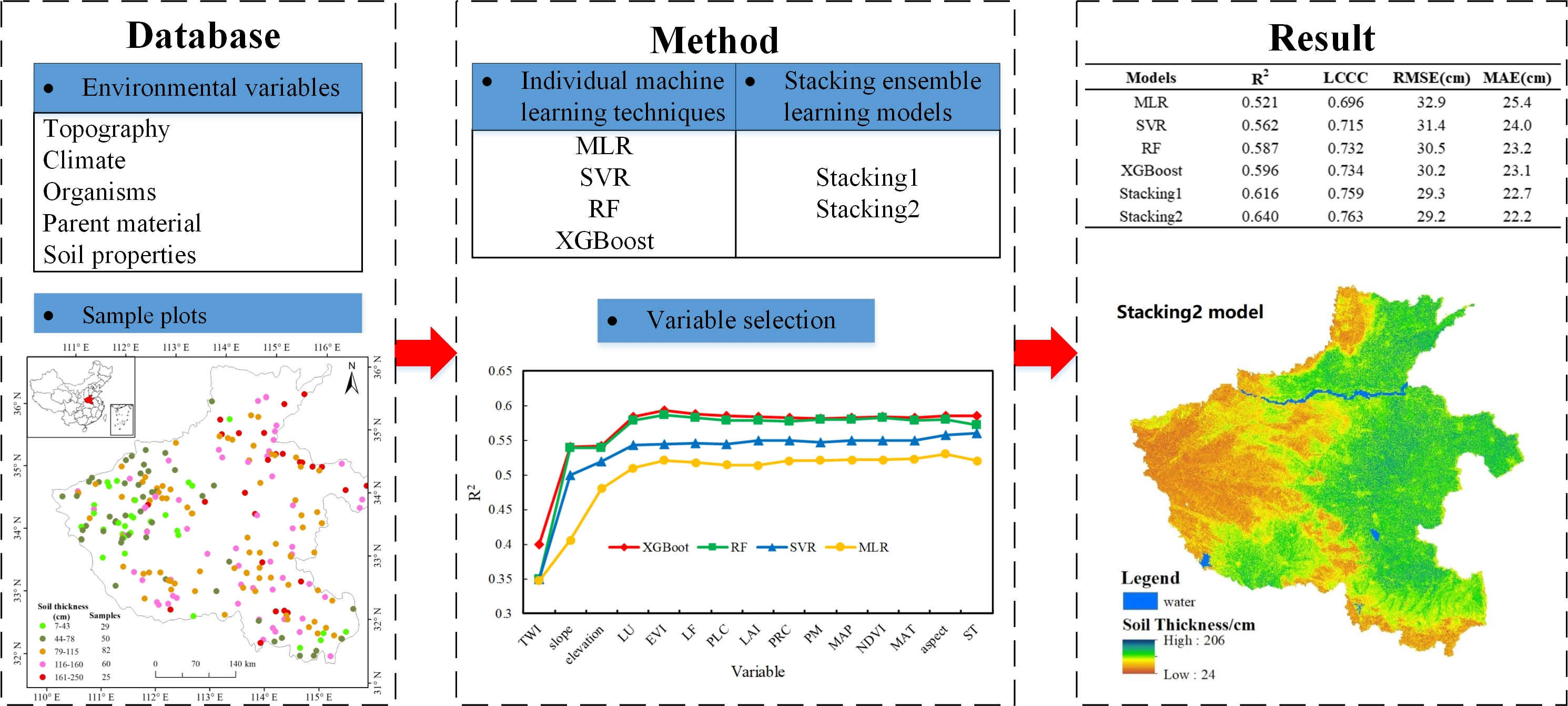
Henan Province is located in central China (Figure 1). The study area lies between latitudes of 110.35° and 116.65° north and between longitudes of 31.37° and 36.37° east with a total area of approximately 167,000 km2. This region has a humid and semi-humid monsoon climate with an average annual temperature ranging from 12.7° to 16.2° and an annual precipitation from 478 mm to 1167 mm. The soil types consist of cinnamon soil, fluro-aquic soil, brown soil and yellow-cinnamon soil [42]. The plain basin and hilly areas account for a total of 55.7% and 44.3% of the region of Henan Province, respectively. Forest and farmland are the dominant land uses in the study area.
2.2. Soil Dataset
Soil thickness is defined, in this study, as the distance from surface to bedrock or material that contains >75% volume of >2 mm gravel [43]. Three available soil datasets were extracted from the work of Wei on soils of Henan Province [44,45]. Detailed information on the landscape, soil profile, soil type, land use and parent material about the sampling sites was employed. A total of 246 soil thickness sample points were collected. The soil thickness values ranged from 7 to 250 cm with a mean of 101.5 cm. The standard deviation and coefficient of variation were 47.5 cm and 46.8%, respectively. The results of the Shapiro–Wilk test (p > 0.05) indicated that soil thickness samples followed a normal distribution.
2.3. Environmental Factors
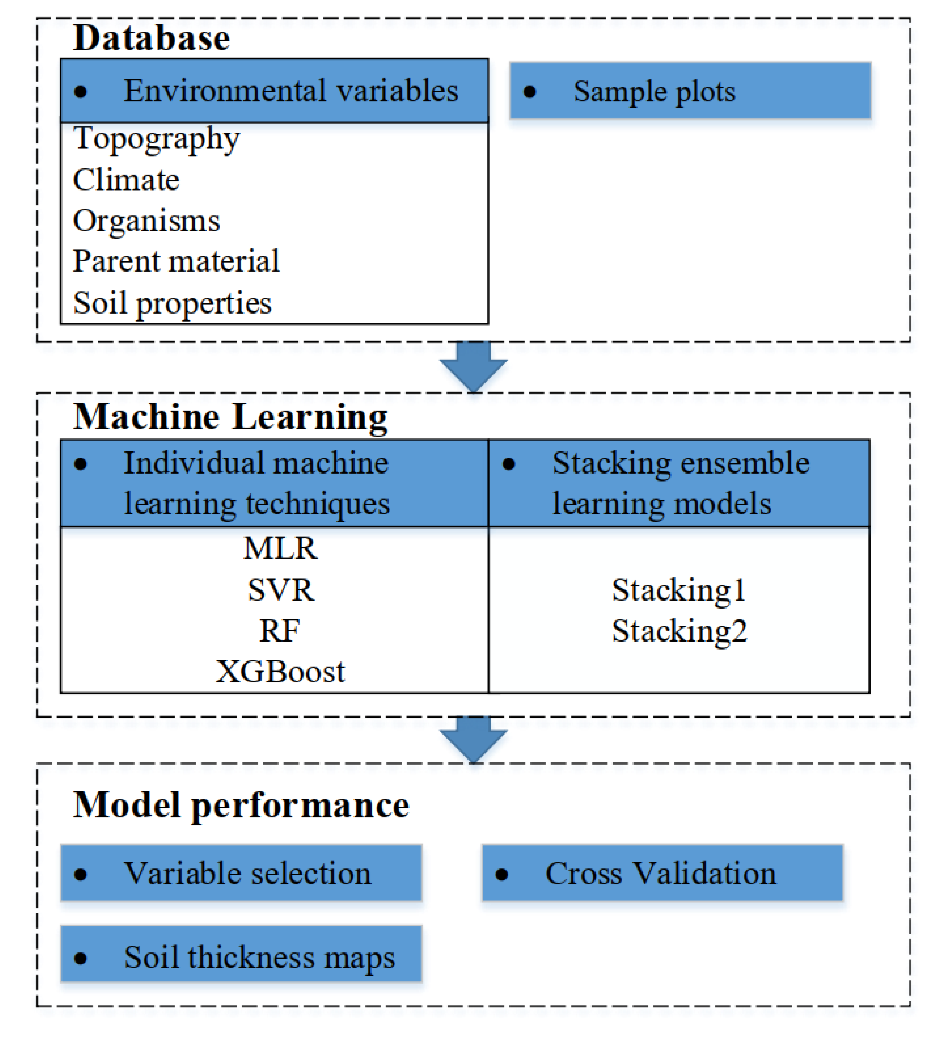
All quantitative and qualitative environmental covariates assumed to influence soil formation were selected (Table 1 and Table 2), including topography, climate, organisms, parent material and soil properties.
2.3.1. Topography
Shuttle Radar Topography Mission (SRTM) digital elevation datasets at 1 arc second (30 m) spatial resolution are widely available from EarthExplorer. Five topographic attributes derived from SRTM DEM were used, including slope, aspect, topographic wetness index (TWI), pan curvature (PLC) and profile curvature (PRC). The System for Automated Geoscientific Analysis (SAGA) was used to derive these topographic attributes [46].
2.3.2. Climate
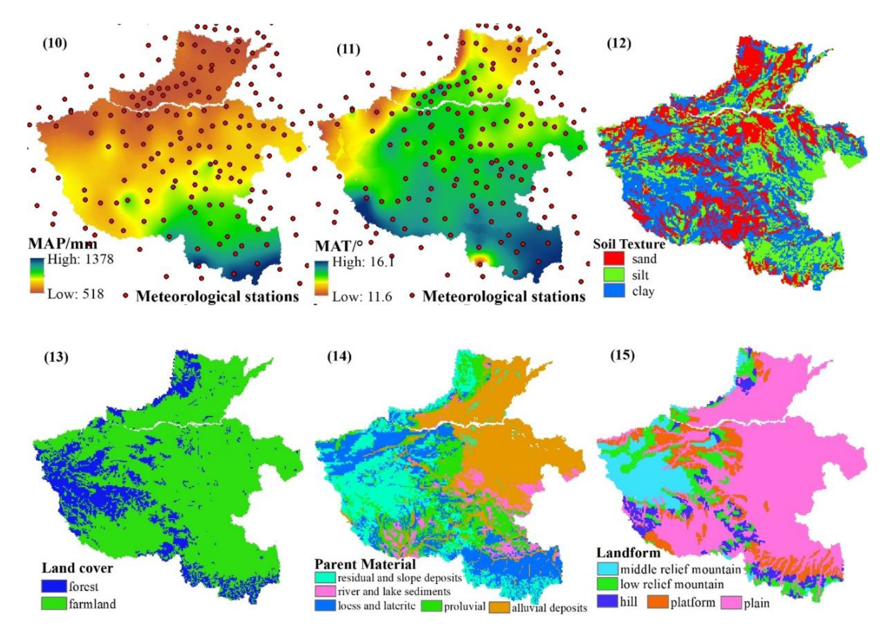
Both mean annual temperature (MAT) and mean annual precipitation (MAP) for the study area from 1980 to 2010 were obtained from China Meteorological Data Sharing Service System (http://data.cma.cn/). MAT and MAP were interpolated over a 250 m grid for 176 meteorological stations using the inverse distance weighting (IDW) interpolation procedure. Mean annual precipitation (MAP) ranges from 518 to 1378 mm, with the average being 766 mm. Mean annual temperature (MAT) ranges from 11.6° to 16.1° mm, with the average being 14.7°.
2.3.3. Vegetation
The normalized difference vegetation index (NDVI), enhanced vegetation index (EVI) and leaf area index (LAI) were used to represent the vegetation conditions of the soil properties. Both NDVI and EVI data were extracted from the MOD13Q1 product from the Moderate-resolution Imaging Spectroradiometer (MODIS) with 250 m spatial resolution and 16-day composites. LAI data were extracted from MOD15A2 with a spatial resolution of 1000 m and 8-day composite. All data were obtained from the Earth Observing System Data and Information System (EOSDIS) (https://search.earthdata.nasa.gov/). This study collected three vegetation products in the period from 2010–2015. First, monthly vegetation data were produced using the maximum value composite (MVC) method [47]. Then, the mean annual NDVI, mean annual EVI and mean annual LAI from 2001 to 2015 were calculated based on monthly vegetation data.
2.3.4. Geological and Soil Environment
We obtained the 1:1,500,000 geological resources and soil environment database of Henan Province from National Earth System Science Data Center (http://www.geodata.cn/). The four quantitative environmental variables used in this work included landform, parent material, soil texture, and land use (Table 2). In order to have sufficient soil thickness samples in each land use category, land use was grouped into forest and farmland.
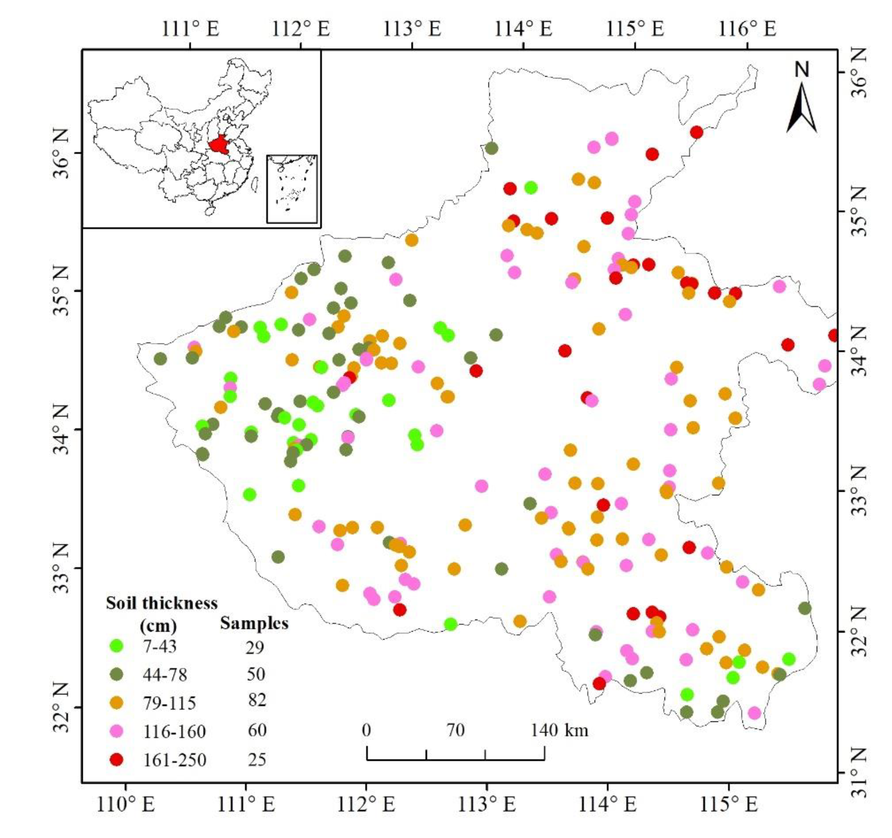
All the covariates were available as raster files. As a processing step, the covariates were resampled to match a 250 m grid using the nearest neighbor strategy. The spatial distributions of 15 environmental variables in this study area are presented in Figure 2.
2.4. Individual Machine Learning Techniques
Numerous machine learning algorithms for digital soil mapping have been provided and discussed [23]. Four commonly used machine learning techniques (MLR, SVR, RF and XGBoost) were compared as individual models in this study.
2.4.1. Multiple Linear Regression
Multiple linear regression (MLR) is one of the simplest machine learning methods to digitally create soil maps [48,49,50], due to its simplicity and efficiency in computation, and easy interpretation. This algorithm finds the best covariates to predict the primary variable (soil thickness) from the explanatory variables (environmental variables) by fitting a linear equation. The MLR was implemented using the lm function in R [51].
2.4.2. Support Vector Regression
Support vector machine (SVM) is a supervised learning method that has recently gained some popularity for predicting soil properties [52]. Support vector regression (SVR) is an extension of SVM, and is used as a regression technique. SVR generates an optimal separating hyperplane to differentiate classes that overlap and are not separable in a linear way. In this case, a large transformed feature space is created to map the data with the help of kernel functions to separate it along a linear boundary. More detailed explanations about SVR can be found in [53]. The commonly used radial basis kernel function was applied in this study. Two parameters of cost and sigma should be defined. After several experiments, the optimal set of cost and sigma is 0.5 and 0.07, respectively. The SVR was implemented using the R package e1071 version 1.7-3 [54].
2.4.3. Random Forest
Random forest (RF) is currently one of the most successful data mining methods in DSM [49]. The principle of RF, randomly selects two-thirds of the training dataset (bootstrapping) to build a decision tree, and the remainder of the training dataset is left out to test the model error using an out-of-bag (OOB) strategy. The RF defines the percent increase in the mean square error (%IncMSE) as the indicator to quantify the importance of the input variables. More detailed explanations about RF can be found in [53]. In RF modeling, the number of trees to grow in the forest (ntree) and the number of variables used per tree (mtry) should be defined. One third of the total number of predictor variables for mtry and ntree = 500 provided stable and visually meaningful results. The RF was implemented using the R package randomForest version 4.6-14 [55].
2.4.4. Extreme Gradient Boosting
Extreme gradient boosting (XGBoost) is a novel tree-based ensemble model proposed by Chen and Guestrin [56]. Based on the boosting strategy, XGBoost can obtain a strong learner from weak learners. The XGBoost algorithm can improve computing speed by parallel learning, prevent over-fitting and improve performance. XGBoost is also able to measure the importance of input variables using the weight. More detailed information about XGBoost can be found in Chen and Guestrin [56]. The XGBoost was implemented using the R package xgboost version 1.1.1.1 [57]. After several experiments, the number of trees (n_estimators) is set as 180, the learning rate is 0.02, the maximum tree depth (max_depth) is 2 and for remaining variables, default parameters were used.
2.5. Stacking Ensemble Learning Models
Four outcomes of MLR, SVR, RF and XGBoost served as an input dataset to the stacking technique that generated the final output. Two stacking ensemble learning models were applied. The first was the least absolute shrinkage and selection operator (LASSO) model (Stacking1), which is a linear model with regularization and avoids over-fitting in the prediction model [58]. The second is the Generalized Boosted Regression Models (GBM) model (Stacking2), which deals with non-linear systems and provides great predictive performance [59]. The glmnet [60] and the gbm [61] packages in R were used to implement the stacking ensemble learning models.
2.6. Model Evaluation
To achieve stable model results, a ten-fold cross validation with 100 repetitions was used to evaluate the prediction performance of different models. Four validation criteria were used to evaluate the prediction accuracy of models: (1) coefficient of determination (R2), (2) root mean square error (RMSE), (3) the mean absolute error (MAE) and (4) Lin's concordance correlation coefficient (LCCC). These indices were calculated as follows:
where Pi and Oi are the predicted and observed soil thickness for the i-th observation; n is the number of sample points; and are the means of the predicted and observed soil thickness values; and are the variances of the predicted and observed values; and r is the Pearson correlation coefficient between the predicted and observed values.
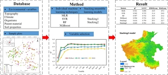
The workflow for digital mapping of soil thickness in this study was shown in Figure 3.
3. Result
3.1. The Relationships between Soil Thickness and Environmental Factors
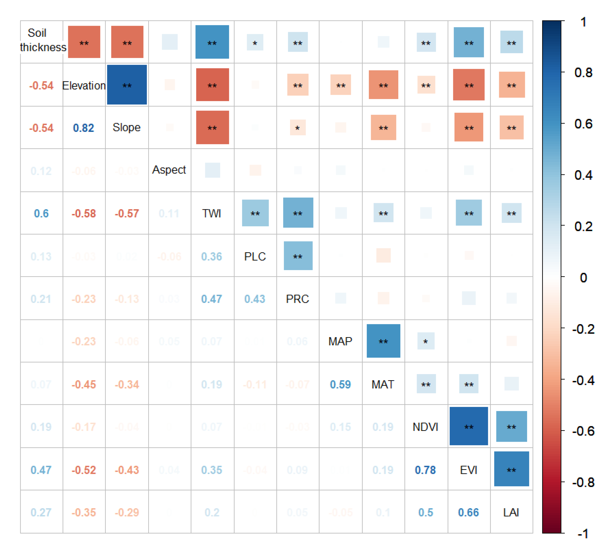
The Pearson correlation matrix between soil thickness and eleven quantitative environmental variables was shown in Figure 4. Soil thickness was positively correlated with TWI (r = 0.60, p < 0.01), PRC (r = 0.21, p < 0.01), NDVI (r = 0.19, p < 0.01), EVI (r = 0.47, p < 0.01), LAI (r = 0.27, p < 0.01), and PLC (r = 0.13, p < 0.05), but negatively correlated with elevation (r = −0.54, p < 0.01) and slope (r = −0.54, p < 0.01). All variables were strongly related to soil thickness, except the aspects MAP and MAT.
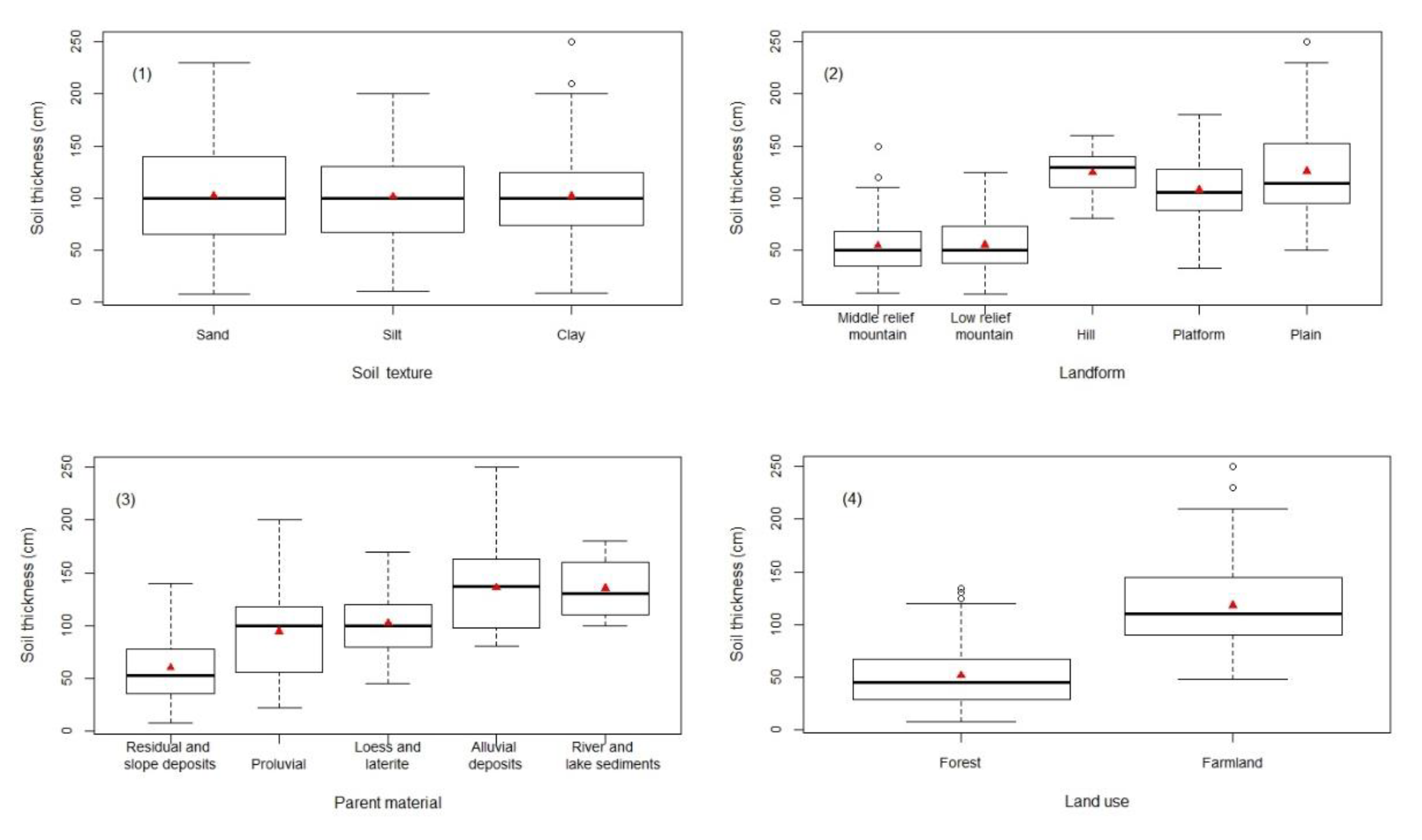
Figure 5 describes the distribution characteristics of soil thickness on four qualitative environmental variables at different classes. The soil thickness values of three soil textures (sand, silt and clay) had similar distributions. There were significant differences in the soil thickness of five landform categories, five parent material categories and two land-use categories. The soil thickness values increased with an increase from middle relief mountain to plain in landform categories. Similarly, each parent material category had a linear effect on soil thickness. The mean soil thickness value of forest was lower than that of farmland in land use.
3.2. Performances of Four Individual Machine Learning (ML) Models
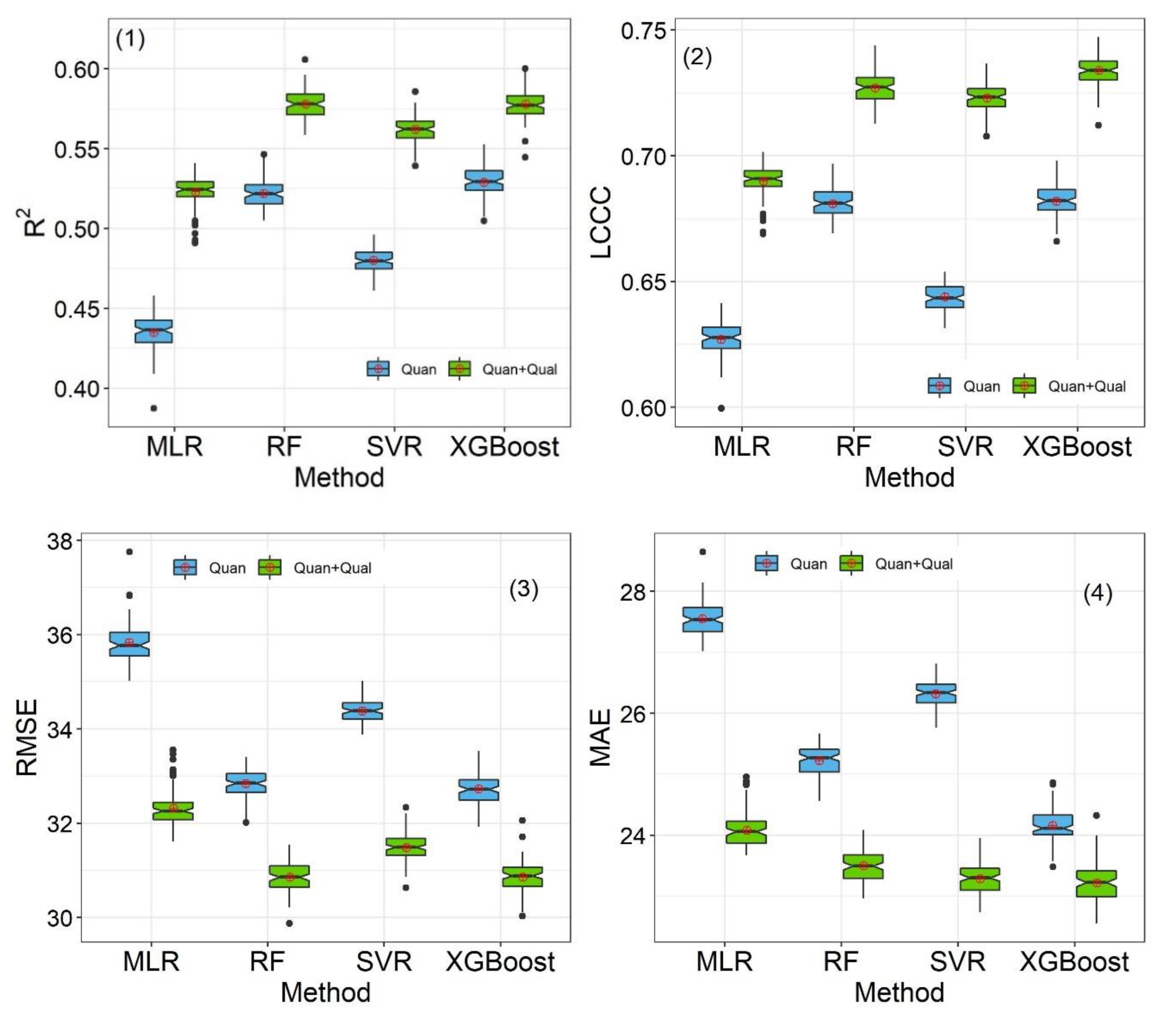
Eleven quantitative environmental variables and four qualitative variables (LF, LU, PM and ST) were used to train four individual ML models: MLR, SVR, RF and XGBoost. To further illustrate the stable performances of these four models, we used boxplots of the R2, LCCC, RMSE and MAE distributions based on 100 iterations (Figure 6). The results showed that the average R2 values of four models using eleven quantitative variables ranged from 0.43 to 0.53; LCCC ranged from 0.63 to 0.68; RMSE was between 32.7 and 35.8 cm; MAE ranged from 24.2 to 27.6 cm. The XGBoost model obtained the best performance to predict soil thickness (R2 = 0.53, LCCC = 0.68, RMSE = 32.7 cm and MAE = 24.2 cm), followed by RF, SVR and MLR.
Incorporation of four qualitative variables improved soil thickness predictions in these four individual ML models. For example, the XGBoost model improved the predictive performance by increasing the R2 and LCCC by 9.15% and 7.57%, respectively, while also reducing the RMSE and MAE by 5.72% and 3.9%, respectively.
3.3. Best Environmental Variables
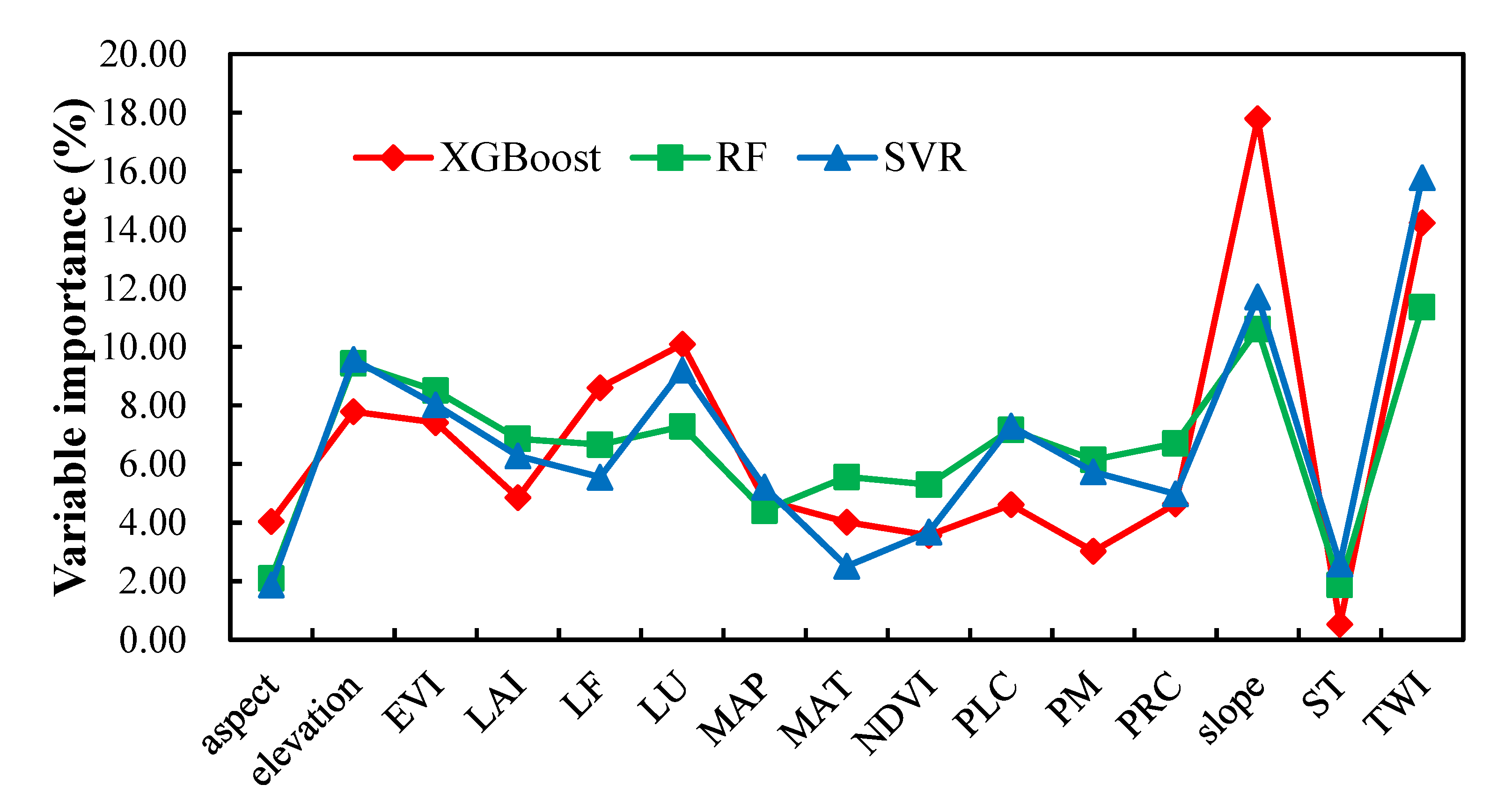
The relative importance of 15 environmental variables in the XGBoost, RF and SVR models were assessed by normalizing the environmental variables of each model to 100% (Figure 7). Three models showed similar environmental variable importance. The five most important predictor variables in the XGBoost model were slope, TWI, LU, LF and elevation. According to the RF model, they were TWI, slope, elevation, LU, and EVI. In the SVR model, they were TWI, lope, elevation, EVI and LU. Generally, TWI and slope were the most critical variables for determining soil thickness. The following important predictor variables varied, but their difference was insignificant. Based on the average rankings of three methods, the variables were ranked in the order of TWI > Slope > Elevation > LU > EVI > LF > PM > PRC > PLC > MAT > LAI > NDVI > MAP > Aspect > ST. In total, the topography exhibited the highest explanation (57.5%, with seven variables) in the soil thickness model, followed by organisms (27.0%, with four variates), climate (8.8%, with two variables), parent material (5.0%, with one variable); and soil (1.7%, with one variable).
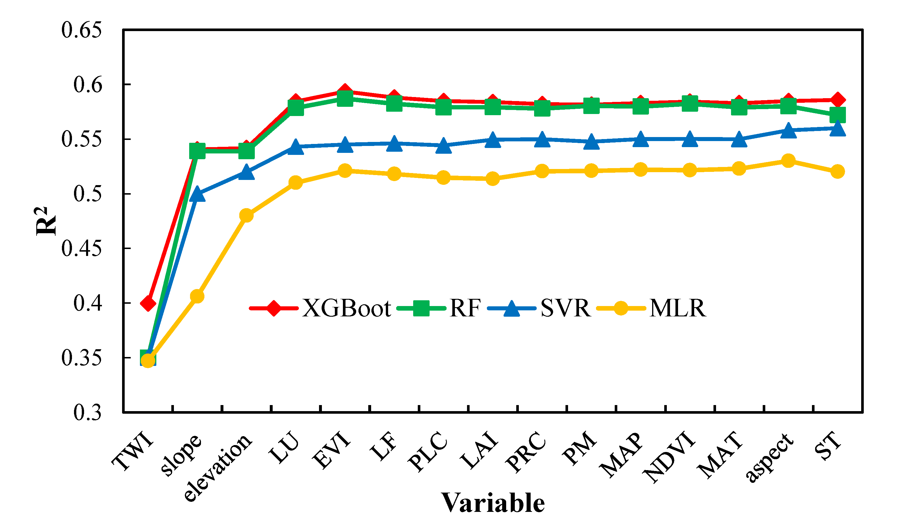
To identify the variations in the predictive accuracies with different numbers of environmental variables using MLR, SVR, RF and XGBoost, we used a forward variable selection approach based on the ranked variables above. Figure 8 shows how R2 values vary with the number of input environmental variables for the MLR, SVR, RF and XGBoost models. The four models had similar variations in that their R2 values increased progressively for each additional input variable. The models comprising the first five variables (TWI, slope, LU, EVI and elevation) were sufficient to reach the highest R2 values of the graph, and the subsequent additional input variables resulted in only very small increases in R2. The inclusion of some redundant variables (such as LF) may cause noise that reduced the robustness of the predicted models. This result indicated that the use of only a few important variables was sufficient to achieve a high level of estimation accuracy.
3.4. Performances of Stacking Ensemble Models
On the basis of the selection of the five best variables (TWI, slope, LU, EVI and elevation), the performances of four individual ML models (MLR, SVR, RF and XGBoost) and two stacking models (Stacking1 and Stacking2) are presented in Table 3. The model accuracy was as follows: Stacking2 > Stacking1 > XGBoost > RF > SVR > MLR. Two stacking approaches had higher accuracy than individual ML models. For instance, the R2 values of Stacking2 and Stacking1 were 7.4% and 3.3% higher than XGBoost, respectively. The Stacking2 model exhibited the greatest performance and could explain 58.7% of the soil thickness variation, with the highest R2 (0.640) and LCCC (0.763) values and the lowest RMSE (29.2 cm) and MAE (22.2 cm) values.
3.5. Spatial Distribution of Soil Thickness
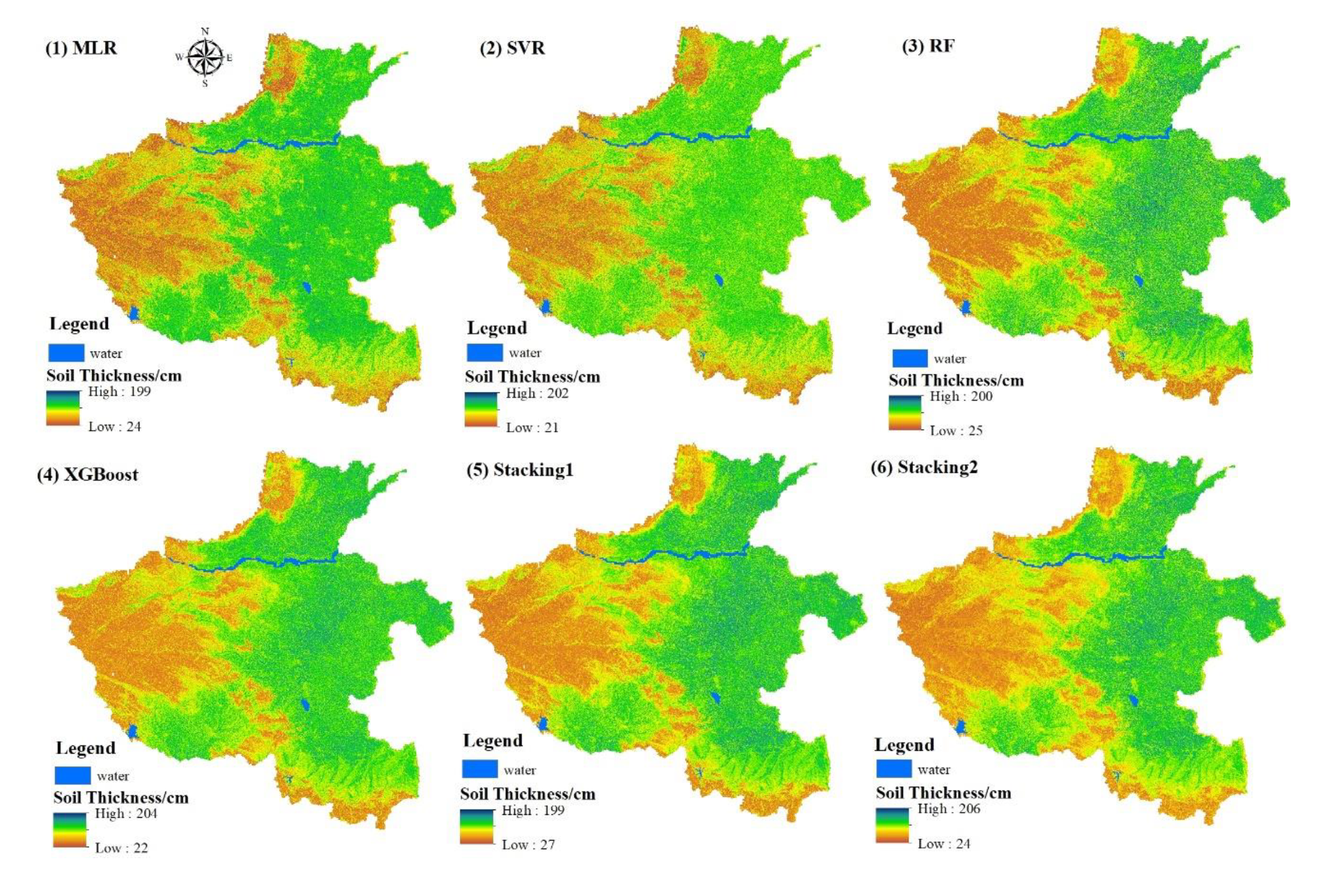
The spatial distribution maps and corresponding descriptive statistics of soil thickness predicted by different models (MLR, SVR, RF, XGBoost, Stacking1 and Stacking2) are shown in Figure 9 and Table 4, respectively. These predicted soil thickness maps had similar spatial distributional trends of soil thickness (Figure 9). Thin soil thickness values were mainly distributed in the western and southern parts of the research area where mountains dominated the landscape. Thick soil thickness values were mainly distributed in the wide plain in the central-eastern and southwest regions. These results showed that the spatial distributions of soil thickness varied significantly with topographic position. The mean values of soil thickness predicted ranged from 99.6 to 105.5 cm, respectively, which were close to the measured values (Table 4).
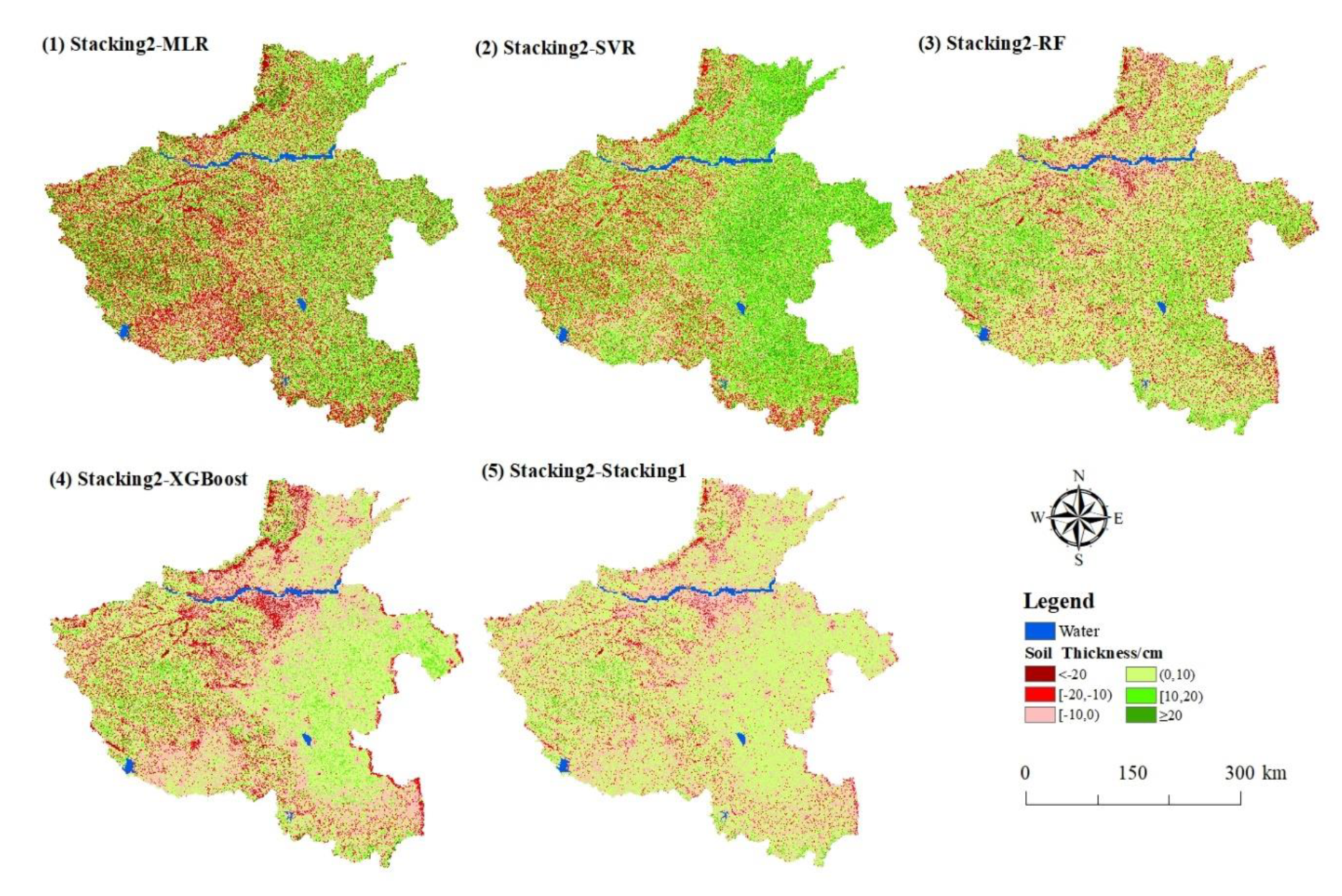
Figure 10 and Table 5 display the differences in the predicted soil thickness maps between the Stacking2 model and the other five models (MLR, SVR, RF, XGBoost, Stacking1). The MLR model and the SVR model had the most significant differences with the Stacking2 model in the predictions results, where their standard deviations were more than 19.1 cm and their differences less than 10 cm were less than 50 %. Most of the differences between the Stacking2 model and the RF and the XGBoost models were less than 10 cm. The Stacking2 model and the Stacking1 model had the smallest spatial distribution differences, of these 91.3% were less than 10 cm. In general, the larger differences of predicted soil thickness maps were mainly located in relatively large topographic variation areas such as steep hillsides, mountain ridges and river valleys, whereas the regions with gentle slopes or low elevations had smaller differences.
4. Discussion
4.1. The Performance of Environmental Variables
According to soil formative factors of the SCORPAN model [12], a total of fifteen relative environmental variables from five factors (soil, climate, organism, topography and parent material) were assembled to explain spatial variability of soil thickness in Henan Province, China.
Findings in previous works coincide with our results in the sense that topography was the main predictor in soil thickness modeling [21,24,62]. Of the topographical variables used in the study, TWI, elevation and slope had highly significant correlations with soil thickness and were the most influential variables in the soil thickness models. We also found that LF was a combination of topography and could reflect the trend of soil thickness variation, which showed significant correlations with soil thickness. The spatial distribution of thick soil thickness was mainly in the floodplains or the bottom of the valleys with low elevations and gentle slopes in this study area. Shallow soil was found in areas of high elevation, steep slopes or rugged relief, where the rate of soil erosion was high. The spatial pattern of soil thickness is a result of the interaction of soil deposition, soil erosion and surface runoff [49]. Soil deposition can be intensified in low plains and valley bottoms and soil erosion is accelerated under increasing elevation in steep areas [29]. TWI reflects the spatial distribution of water flow and thus the accumulation processes in a closed catchment. Yang et al. [50] reported that TWI, slope and elevation explained approximately 61.4% of the variation on soil thickness in karst regions in Southwest China. Ho et al. [63] also showed that TWI was an important variable reflecting the spatial distribution of soil thickness.
The main soil-forming or altering organisms are natural vegetation or humans (e.g., land use) [12]. The soil-vegetation feedback system indicates that the distribution of vegetation is influenced by soil properties [64]. We also demonstrated that vegetation was the main factor affecting soil thickness. EVI, NDVI and LAI have positive correlations with soil thickness. The high vegetation fractional coverage shows that soil can be well protected against soil erosion, resulting in a large soil thickness. EVI provides improved vegetation monitoring through increased sensitivity in areas with dense biomass and reduced atmospheric influences [65]. EVI captured vegetation variations more sensitively compared to NDVI and LAI. Land use was classified as forest and farmland in this study, and it was another indicator of vegetation. The soil thickness values of forest were significantly lower than those of farmland, where the high fractional coverage of vegetation mostly occurred in farmland. The models that used LU made a large contribution to soil thickness modeling. Kuriakose et al. [11] indicated that land use had a strong relationship with soil thickness in the Aruvikkal catchment. Sarkar et al. (2013) stated that land use was identified as the most dominant predictor of soil thickness in the regression analysis.
The nature of the parent material can be a significant influence on soil thickness. We also found that soil thickness values varied with different parent material categories. Additionally, the spatial distributions of topography and parent material were highly consistent in this study area. The soil thickness values increased with an increase from residual and slope deposits to loess and laterite. Chen et al. [66] also indicated that parent material was the most important variable in the soil thickness modeling of mainland France.
Climate may control soil distribution over a continental scale [8]. Malone and Searle [67] found that climatic variables were consistently used and important in mapping soil thickness across Australia. In this study, MAP and MAT had no correlation with soil thickness (p > 0.05) and were not selected as predictors in the modeling. This could be due to the distributions of MAP and MAT that decreased from south to north, which reflects the characteristics of latitude, and these variables have relatively small impacts on the weathering of parent rocks and soil formation in this area [21]. In this study, soil texture showed only weak predictive power in the models. Soil texture was slightly relevant to infer soil thickness variations.
4.2. The Importance of Variable Selection
Variable selection is one of the most important processes in modeling, which can reduce the number of predictor variables to several important variables and make it easier to interpret the model [18]. The inclusion of additional environmental variables potentially adds additional information and is usually expected to improve predictions in DSM. However, different variables showed different predictive capabilities in the soil thickness modeling. This increased dimensionality and complexity may actually result in a decrease in accuracy. We generally observed improvements when using more variables, but the improvements were not large and may be outweighed by the costs. This is because the number of training data may be insufficient to characterize the increased complexity associated with the larger dimensionality of the feature space. The contributions of the other variables were less important and could reduce the model’s performance and capability [68]. RF, SVR and XGBoost models have their own procedures for calculating the importance of each variable. Their importance scores may be different, but most optimal variables selected were similar. This result is in line with other studies [69]. In this study, TWI, slope, LU, EVI and elevation played more important roles than the other variables and achieved the best accuracy, which is consistent with the result of Lu et al. [21] who reported that the performance of four environmental covariates selected by the proposed method was better than that of all 17 variables.
4.3. The Performance of Ensemble Methods
RF and XGBoost are the most popular ensemble methods for bagging and boosting, respectively. They are both based on decision trees and are different with respect to the tree ensemble methods. In this study, the XGBoost model performed slightly better than the RF model based on the comparison of four statistical indicators (R2, LCCC, RMSE and MAE). This is likely due to the differences in the tree ensemble methods. RF uses the bagging (bootstrap resampling) method to build different training sets, and average the forecast results of decisions trees. XGBoost uses previous ideas from gradient boosting, creating tree models based on residuals from previously created trees. Dietterich [70] compared bagging and boosting ensembles and found that boosting outperformed bagging in the dataset with little noise.
These two tree-based models performed much better than SVR and MLR, as they are more capable of dealing with the non-linear problem, resistance to overfitting, and capturing complex interactions in the variables. MLR exhibited poorly performance in this study area because it cannot solve the non-linear relationships between soil attributes and environmental variables. SVR is able to model highly non-linear dimensional relationships, but its performance is still susceptible to overfitting and finding optimal parameters. Scarpone et al. [29] used different models to map the soil thickness in the Tulameen study area in the southern interior of British Columbia and found that the predictive performance of the RF model was significantly better than the generalized linear model. Li et al. [49] compared the accuracy of MLR, geographically weighted regression (GWR), SVR, and RF models to predict active-layer soil thickness, and found that RF performed best and MLR performed worst.
All available information is not always efficiently used by a single accurate model. Each algorithm has specific advantages and disadvantages. The errors of the single model have different uncertainties. The application of the stacking ensemble model used multiple learning models’ strengths to achieve more robust performance, reduce estimation uncertainties and improve prediction accuracy. The stacking strategy was more accurate than individual models in the current research. The predictions from four individual models with different principles were combined using two stacking approaches: LASSO and GBM. The GBM stacking model (Stacking2) achieves better predictive performance than the LASSO stacking model (Stacking1). GBM is more capable of dealing with the non-linear problem, resistance to overfitting, and capturing complex interactions in the variables [71,72].
Several studies have found this advantage for predicting soil properties. For instance, Taghizadeh-Mehrjardi et al. [36] proposed the stacking approach to have the best performances in soil organic carbon (SOC) content predictions in comparison to six ML models. They also found that the RMSE values of stacking models using SVR for SOC content were lower those of stacking models using LASSO. Chen et al. [40] couplied RF and XGBoost models to predict soil pH at the national scale. Román Dobarco et al. [41], however, found that the ensemble predictions did not improve for silt and sand, and improved only for clay. The performance of the stacking models may depend on the quality of input datasets or primary maps and the diversification of the input single models [73,74].
4.4. The Performance of Predictions
The proposed model (Stacking2) found in this study used the five best variables and the stacking ensemble method to explain 64.0% of soil thickness variation. Tesfa et al. [24] used the developed random forest model with 11 input variables to explain approximately 50% of the variation of soil thickness in a semiarid mountainous watershed. Sarkar et al. [23] showed that the regression kriging model with seven landscape variables could explain 67% of the variability of soil thickness in a Himalayan terrain. Lacoste et al. [8] proposed three methods to explain 50–58% of the soil thickness variation in France. Lu et al. [21] used five environmental covariates and the RF method to explain 76% of the variation in soil thickness. Malone and Searle [67] developed an integrated data mining approach to create soil thickness maps across Australia with a concordance coefficient of 0.77. The results described in our research were within the range of previous studies.
The soil thickness maps predicted by different models exhibited similar distribution patterns, and topography was the most notable variable. Thick soil was mostly concentrated in valleys, wide plains and areas with gentle slopes, while thin soil was mainly found in steep slopes and areas of high elevation. Topography was shown to be the dominant factor of soil thickness in these landscapes. This result was also consistent with other studies [8,11,49]. Our results indicated that the predicted soil thickness was less variable than the measured soil thickness. Similar findings were also reported in soil thickness mapping studies by Yang et al. [50]
4.5. Limitations and Future Research
First, it was difficult to assess the uncertainty of the quantitative environmental variables with coarse resolutions, which were surveyed during the Second National Soil Survey of China [75]. Therefore, it is necessary to explore the influence of more detailed environmental variables in soil thickness mapping [76]. Other environmental variables such as vegetation types, bedrock geology and soil type should be explored [77,78]. Second, machine learning approaches discover and quantify only the relationships between soil thickness and environmental variables and ignore the neighbouring spatial information of soil sample sites for DSM. The combination of regression models and geostatistical methods such as kriging could account for more of the variability in the landscape, and thus has led to improvements in DSM [29]. Different validation strategies (such as block cross validation) should be applied to test model performance because of the over-fitting in machine learning models [79,80,81]. Third, the main factors controlling soil thickness may not be the same at different spatial and temporal scales [75] and the optimal spatial resolution for soil thickness prediction should be discussed [25].
5. Conclusions
In this study, exhaustive covariates and machine learning methods were applied to build the most reliable and accurate estimation model to provide the spatial distribution of soil thickness for Henan Province in China. The results suggested that using qualitative environmental variables could improve the accuracy of soil thickness estimations; in particular, each qualitative variable category showed significant differences with soil thickness values. The results also demonstrated the importance of variable selection in soil thickness modeling. Topography and organisms were the most important environmental soil-forming factors in predicting soil thickness. After variable selection, TWI, slope, elevation, land use and EVI were the most important environmental variables explaining the observed variability in soil thickness. Out of four individual machine learning methods, XGBoost achieved the best performance, followed by RF, SVR, and MLR. However, compared with these individual methods, two stacking models showed better performance. The best model (Stacking2) exhibited the greatest performance with the highest R2 (0.640) and LCCC (0.763) values and the lowest RMSE (29.2 cm) and MAE (22.2 cm) values. From the soil thickness spatial distribution maps, thick soils were mainly concentrated in valleys and low elevations and shallow soils mostly occurred on steep slopes and high elevations. This study provided an example of producing regional soil thickness maps. It is recommended to select appropriate variables and stacking models when using machine learning algorithms for digital soil mapping.
Author Contributions
Conceptualization: X.L., J.L. and X.J.; methodology: X.J. and X.L.; formal analysis: X.L., J.L. and Q.H.; writing—original draft preparation: X.L., X.J. and Q.H.; writing—review and editing: X.L., X.J. and Y.N.; supervision: J.L. and Y.N.; funding acquisition: X.L. and J.L. All authors have read and agreed to the published version of the manuscript.
Funding
This work was funded jointly by the National Natural Science Foundation of China (41801075); the China Postdoctoral Science Foundation (2018M642349); Funded by Key Laboratory of Watershed Geographic Sciences, Nanjing Institute of Geography and Limnology, Chinese Academy of Sciences (WSGS2017009); Natural Science Foundation Project of Universities and Institutes in Jiangsu Province (18KJB170002).
Acknowledgments
We acknowledge the support provided by the National Earth System Science Data Center, National Science and Technology Infrastructure of China for providing the geological resources and soil environment database (http://www.geodata.cn).
Conflicts of Interest
The authors declare no conflict of interest.
References
- Vogel, H.; Bartke, S.; Daedlow, K.; Helming, K.; Kögel-Knabner, I.; Lang, B.; Rabot, E.; Russell, D.; Stößel, B.; Weller, U.; et al. A systemic approach for modeling soil functions. Soil 2018, 4, 83–92. [Google Scholar] [CrossRef] [Green Version]
- Meyer, M.D.; North, M.P.; Gray, A.N.; Harold, S.J.Z. Influence of soil thickness on stand characteristics in a Sierra Nevada mixed-conifer forest. Plant Soil. 2007, 294, 113–123. [Google Scholar] [CrossRef]
- Gochis, D.J.; Vivoni, E.R.; Watts, C.J. The impact of soil depth on land surface energy and water fluxes in the North American Monsoon region. J. Arid Environ. 2010, 74, 564–571. [Google Scholar] [CrossRef]
- Liang, W.; Chan, M. Spatial and temporal variations in the effects of soil depth and topographic wetness index of bedrock topography on subsurface saturation generation in a steep natural forested headwater catchment. J. Hydrol. 2017, 546, 405–418. [Google Scholar] [CrossRef]
- Chan, H.C.; Chang, C.C.; Chen, P.A.; Lee, J.T. Using multinomial logistic regression for prediction of soil depth in an area of complex topography in Taiwan. Catena 2019, 176, 419–429. [Google Scholar] [CrossRef]
- Zhang, G.; Liu, F.; Song, X. Recent progress and future prospect of digital soil mapping: A review. J. Integr. Agric. 2017, 16, 2871–2885. [Google Scholar] [CrossRef]
- Hartemink, A.E.; McBratney, A. A soil science renaissance. Geoderma 2008, 148, 123–129. [Google Scholar] [CrossRef]
- Lacoste, M.; Mulder, V.L.; Richer-de-Forges, A.C.; Martin, M.P.; Arrouays, D. Evaluating large-extent spatial modeling approaches: A case study for soil depth for France. Geoderma Reg. 2016, 7, 137–152. [Google Scholar] [CrossRef]
- Minasny, B.; McBratney, A.B. Digital soil mapping: A brief history and some lessons. Geoderma 2016, 264, 301–311. [Google Scholar] [CrossRef]
- Savin, I.Y.; Zhogolev, A.V.; Prudnikova, E.Y. Modern Trends and Problems of Soil Mapping. Eurasian Soil Sci. 2019, 52, 471–480. [Google Scholar] [CrossRef]
- Kuriakose, S.L.; Devkota, S.; Rossiter, D.G.; Jetten, V.G. Prediction of soil depth using environmental variables in an anthropogenic landscape, a case study in the Western Ghats of Kerala, India. Catena 2009, 79, 27–38. [Google Scholar] [CrossRef]
- McBratney, A.B.; Mendonça Santos, M.L.; Minasny, B. On digital soil mapping. Geoderma 2003, 117, 3–52. [Google Scholar] [CrossRef]
- Jafari, A.; Finke, P.A.; Vande Wauw, J.; Ayoubi, S.; Khademi, H. Spatial prediction of USDA- great soil groups in the arid Zarand region, Iran: Comparing logistic regression approaches to predict diagnostic horizons and soil types. Eur. J. Soil Sci. 2012, 63, 284–298. [Google Scholar] [CrossRef]
- Zeraatpisheh, M.; Jafari, A.; Bagheri Bodaghabadi, M.; Ayoubi, S.; Taghizadeh-Mehrjardi, R.; Toomanian, N.; Kerry, R.; Xu, M. Conventional and digital soil mapping in Iran: Past, present, and future. Catena 2020, 188, 104424. [Google Scholar] [CrossRef]
- Cavazzi, S.; Corstanje, R.; Mayr, T.; Hannam, J.; Fealy, R. Are fine resolution digital elevation models always the best choice in digital soil mapping? Geoderma 2013, 195–196, 111–121. [Google Scholar] [CrossRef]
- Hengl, T.; Nikolić, M.; MacMillan, R.A. Mapping efficiency and information content. Int. J. Appl. Earth Obs. 2013, 22, 127–138. [Google Scholar] [CrossRef]
- Kim, J.S.; Grunwald, S.; Rivero, R.G. Soil Phosphorus and Nitrogen Predictions Across Spatial Escalating Scales in an Aquatic Ecosystem Using Remote Sensing Images. IEEE Trans. Geosci. Remote Sens. 2014, 52, 6724–6737. [Google Scholar] [CrossRef]
- Li, Y.; Chao, L.; Li, M. Influence of Variable Selection and Forest Type on Forest Aboveground Biomass Estimation Using Machine Learning Algorithms. Forests 2019, 10, 1073. [Google Scholar] [CrossRef] [Green Version]
- Samuel-Rosa, A.; Heuvelink, G.B.M.; Vasques, G.M.; Anjos, L.H.C. Do more detailed environmental covariates deliver more accurate soil maps? Geoderma 2015, 243–244, 214–227. [Google Scholar] [CrossRef]
- Tien Bui, D.; Tuan, T.A.; Klempe, H.; Pradhan, B.; Revhaug, I. Spatial prediction models for shallow landslide hazards: A comparative assessment of the efficacy of support vector machines, artificial neural networks, kernel logistic regression, and logistic model tree. Landslides 2016, 13, 361–378. [Google Scholar] [CrossRef]
- Lu, Y.; Liu, F.; Zhao, Y.; Song, X.; Zhang, G. An integrated method of selecting environmental covariates for predictive soil depth mapping. J. Integr. Agric. 2019, 18, 301–315. [Google Scholar] [CrossRef]
- Emadi, M.; Taghizadeh-Mehrjardi, R.; Cherati, A.; Danesh, M.; Mosavi, A.; Scholten, T. Predicting and Mapping of Soil Organic Carbon Using Machine Learning Algorithms in Northern Iran. Remote Sens. 2020, 12, 2234. [Google Scholar] [CrossRef]
- Sarkar, S.; Roy, A.K.; Martha, T.R. Soil depth estimation through soil-landscape modelling using regression kriging in a Himalayan terrain. Int. J. Geogr. Inf. Sci. 2013, 27, 2436–2454. [Google Scholar] [CrossRef]
- Tesfa, T.K.; Tarboton, D.G.; Chandler, D.G.; Mcnamara, J.P. Modeling soil depth from topographic and land cover attributes. Water Resour. Res. 2009, 45, W10438. [Google Scholar] [CrossRef]
- Han, X.; Liu, J.; Mitra, S.; Li, X.; Srivastava, P.; Guzman, S.M.; Chen, X. Selection of optimal scales for soil depth prediction on headwater hillslopes: A modeling approach. Catena 2018, 163, 257–275. [Google Scholar] [CrossRef]
- Zhou, T.; Geng, Y.; Chen, J.; Sun, C.; Haase, D.; Lausch, A. Mapping of Soil Total Nitrogen Content in the Middle Reaches of the Heihe River Basin in China Using Multi-Source Remote Sensing-Derived Variables. Remote Sens. 2019, 11, 2934. [Google Scholar] [CrossRef] [Green Version]
- Li, J.; Heap, A.D.; Potter, A.; Daniell, J.J. Application of machine learning methods to spatial interpolation of environmental variables. Environ. Modell. Softw. 2011, 26, 1647–1659. [Google Scholar] [CrossRef]
- Khaledian, Y.; Miller, B.A. Selecting appropriate machine learning methods for digital soil mapping. Appl. Math. Model. 2020, 81, 401–418. [Google Scholar] [CrossRef]
- Scarpone, C.; Schmidt, M.G.; Bulmer, C.E.; Knudby, A. Modelling soil thickness in the critical zone for Southern British Columbia. Geoderma 2016, 282, 59–69. [Google Scholar] [CrossRef]
- Keskin, H.; Grunwald, S.; Harris, W.G. Digital mapping of soil carbon fractions with machine learning. Geoderma. 2019, 339, 40–58. [Google Scholar] [CrossRef]
- Sagi, O.; Rokach, L. Ensemble learning: A survey. Wiley Interdiscip. Rev. Data Min. Knowl. Discov. 2018, 8. [Google Scholar] [CrossRef]
- Opitz, D.; Maclin, R. Popular Ensemble Methods: An Empirical Study. J Artif. Intell. Res. 1999, 11, 169–198. [Google Scholar] [CrossRef]
- Song, X.; Wu, H.; Ju, B.; Liu, F.; Yang, F.; Li, D.; Zhao, Y.; Yang, J.; Zhang, G. Pedoclimatic zone-based three-dimensional soil organic carbon mapping in China. Geoderma 2020, 363, 114145. [Google Scholar] [CrossRef]
- Riggers, C.; Poeplau, C.; Don, A.; Bamminger, C.; Höper, H.; Dechow, R. Multi-model ensemble improved the prediction of trends in soil organic carbon stocks in German croplands. Geoderma 2019, 345, 17–30. [Google Scholar] [CrossRef]
- Chen, S.; Mulder, V.L.; Heuvelink, G.B.M.; Poggio, L.; Caubet, M.; Román Dobarco, M.; Walter, C.; Arrouays, D. Model averaging for mapping topsoil organic carbon in France. Geoderma 2020, 366, 114237. [Google Scholar] [CrossRef]
- Taghizadeh-Mehrjardi, R.; Schmidt, K.; Amirian-Chakan, A.; Rentschler, T.; Zeraatpisheh, M.; Sarmadian, F.; Valavi, R.; Davatgar, N.; Behrens, T.; Scholten, T. Improving the Spatial Prediction of Soil Organic Carbon Content in Two Contrasting Climatic Regions by Stacking Machine Learning Models and Rescanning Covariate Space. Remote Sens. 2020, 12, 1095. [Google Scholar] [CrossRef] [Green Version]
- Pham, B.T.; Prakash, I.; Singh, S.K.; Shirzadi, A.; Shahabi, H.; Tran, T.; Bui, D.T. Landslide susceptibility modeling using Reduced Error Pruning Trees and different ensemble techniques: Hybrid machine learning approaches. Catena 2019, 175, 203–218. [Google Scholar] [CrossRef]
- Zhou, Y.; Xue, J.; Chen, S.; Zhou, Y.; Liang, Z.; Wang, N.; Shi, Z. Fine-Resolution Mapping of Soil Total Nitrogen across China Based on Weighted Model Averaging. Remote Sens. 2020, 12, 85. [Google Scholar] [CrossRef] [Green Version]
- Taghizadeh-Mehrjardi, R.; Minasny, B.; Toomanian, N.; Zeraatpisheh, M.; Amirian-Chakan, A.; Triantafilis, J. Digital Mapping of Soil Classes Using Ensemble of Models in Isfahan Region, Iran. Soil Syst. 2019, 3, 37. [Google Scholar] [CrossRef] [Green Version]
- Chen, S.; Liang, Z.; Webster, R.; Zhang, G.; Zhou, Y.; Teng, H.; Hu, B.; Arrouays, D.; Shi, Z. A high-resolution map of soil pH in China made by hybrid modelling of sparse soil data and environmental covariates and its implications for pollution. Sci. Total Environ. 2019, 655, 273–283. [Google Scholar] [CrossRef] [PubMed]
- Román Dobarco, M.; Arrouays, D.; Lagacherie, P.; Ciampalini, R.; Saby, N.P.A. Prediction of topsoil texture for Region Centre (France) applying model ensemble methods. Geoderma 2017, 298, 67–77. [Google Scholar] [CrossRef]
- Ren, Y.; Zhang, X. Multi-class Geomorphic Diversity and Its Relationship with Pedodiversity in Henan Province. Soils 2019, 51, 142–151. (In Chinese) [Google Scholar]
- Yi, C.; Li, D.; Zhang, G.; Zhao, Y.; Yang, J.; Liu, F.; Song, D. Criteria for partition of soil thickness and case studies. Acta Pedol. Sin. 2015, 52, 220–227. (In Chinese) [Google Scholar]
- Wei, K. Soil Geography of Henan; Henan Science and Technology Press: Zhengzhou, China, 1995. (In Chinese) [Google Scholar]
- Wei, K. Soils of Henan Province; China Agriculture Press: Beijing, China, 2004. (In Chinese) [Google Scholar]
- Conrad, O.; Olaya, V. SAGA-GIS Module Library Documentation (v2.2.3). Module Valley Depth. Available online: http://www.sagagis.org/saga_tool_doc/2.2.3/index.html (accessed on 2 January 2020).
- Piao, S.; Jingyun, F.; Zhou, L.; Qinghua, G.; Henderson, M.; Wei, J.; Yan, L.; Shu, T. Interannual variations of monthly and seasonal normalized difference vegetation index (NDVI) in China from 1982 to 1999. J. Geophys. Res. 2003, 108. [Google Scholar] [CrossRef]
- Mehnatkesh, A.; Ayoubi, S.; Jalalian, A.; Sahrawat, K.L. Relationships between Soil Depth and Terrain Attributes in a Semi Arid Hilly Region in Western Iran. J. Mt. Sci. 2013, 10, 163–172. [Google Scholar] [CrossRef]
- Li, A.; Tan, X.; Wu, W.; Liu, H.; Zhu, J. Predicting active-layer soil thickness using topographic variables at a small watershed scale. PLoS ONE 2017, 12, e183742. [Google Scholar] [CrossRef]
- Yang, Q.; Zhang, F.; Jiang, Z.; Li, W.; Zhang, J.; Zeng, F.; Li, H. Relationship between soil depth and terrain attributes in karst region in Southwest China. J. Soils Sediment 2014, 14, 1568–1576. [Google Scholar] [CrossRef]
- R Core Team. R: A Language and Environment for Statistical Computing, R Foundation for Statistical Computing, Vienna, Austria. Available online: http://www.R-project.org (accessed on 12 December 2019).
- Lamichhane, S.; Kumar, L.; Wilson, B. Digital soil mapping algorithms and covariates for soil organic carbon mapping and their implications: A review. Geoderma 2019, 352, 395–413. [Google Scholar] [CrossRef]
- Breiman, L. Random forests. Mach. Learn. 2001, 45, 5–32. [Google Scholar] [CrossRef] [Green Version]
- Meyer, D.; Wien, F.T. Support Vector Machines—The Interface to Libsvm in Package e1071. Available online: https://cran.r-project.org/web/packages/e1071/index.html (accessed on 25 November 2019).
- Breiman, L.; Cutler, A. Breiman and Cutler’s Random Forests for Classification and Regression. Available online: https://cran.r-project.org/web/packages/randomForest/ (accessed on 25 March 2018).
- Chen, T.; Guestrin, C. XGBoost: A Scalable Tree Boosting System. In Proceedings of the 22nd ACM SIGKDD International Conference on Knowledge Discovery and Data Mining; ACM: New York, NY, USA, 2016; pp. 785–794. [Google Scholar]
- Chen, T.; He, T.; Benesty, M.; Khotilovich, V.; Tan, Y. Extreme Gradient Boosting. 2020. Available online: https://cran.r-project.org/web/packages/xgboost/xgboost.pdf. (accessed on 30 July 2020).
- Friedman, J.; Hastie, T.; Tibshirani, R. Regularization Paths for Generalized Linear Models via Coordinate Descent. J. Stat. Softw. 2010, 33, 1–22. [Google Scholar] [CrossRef] [Green Version]
- Friedman, J.H. Greedy Function Approximation: A Gradient Boosting Machine. Ann. Stat. 2001, 29, 1189–1232. [Google Scholar] [CrossRef]
- Friedman, J.; Hastie, T.; Tibshirani, R.; Narasimhan, B.; Tay, K.; Simon, N.; Qian, J. Lasso and Elastic-Net Regularized Generalized Linear Models. Available online: https://cran.r-project.org/web/packages/glmnet/index.html (accessed on 30 July 2020).
- Ridgeway, G. Gbm: Generalized Boosted Regression Models. Available online: https://cran.r-project.org/web/packages/gbm/index.html (accessed on 30 July 2020).
- Gessler, P.E.; Chadwick, O.A.; Chamran, F.; Holmes, K. Modeling soil-landscape and ecosystem properties using terrain attributes. Soil Sci. Soc. Am. J. 2000, 64, 2046–2050. [Google Scholar] [CrossRef] [Green Version]
- Ho, J.; Lee, K.T.; Chang, T.; Wang, Z.; Liao, Y. Influences of spatial distribution of soil thickness on shallow landslide prediction. Eng. Geol. 2012, 124, 38–46. [Google Scholar] [CrossRef]
- Maynard, J.J.; Levi, M.R. Hyper-temporal remote sensing for digital soil mapping: Characterizing soil-vegetation response to climatic variability. Geoderma 2017, 285, 94–109. [Google Scholar] [CrossRef] [Green Version]
- Swain, S.; Abeysundara, S.; Hayhoe, K.; Stoner, A.M.K. Future changes in summer MODIS-based enhanced vegetation index for the South-Central United States. Ecol. Inform. 2017, 41, 64–73. [Google Scholar] [CrossRef]
- Chen, S.; Mulder, V.L.; Martin, M.P.; Walter, C.; Lacoste, M.; Richer-de-Forges, A.C.; Saby, N.P.A.; Loiseau, T.; Hu, B.; Arrouays, D. Probability mapping of soil thickness by random survival forest at a national scale. Geoderma 2019, 344, 184–194. [Google Scholar] [CrossRef]
- Malone, B.; Searle, R. Improvements to the Australian national soil thickness map using an integrated data mining approach. Geoderma 2020, 377, 114579. [Google Scholar] [CrossRef]
- Paul, S.S.; Coops, N.C.; Johnson, M.S.; Krzic, M.; Chandna, A.; Smukler, S.M. Mapping soil organic carbon and clay using remote sensing to predict soil workability for enhanced climate change adaptation. Geoderma 2020, 363, 114177. [Google Scholar] [CrossRef]
- Wang, B.; Waters, C.; Orgill, S.; Cowie, A.; Clark, A.; Li Liu, D.; Simpson, M.; McGowen, I.; Sides, T. Estimating soil organic carbon stocks using different modelling techniques in the semi-arid rangelands of eastern Australia. Ecol. Indic. 2018, 88, 425–438. [Google Scholar] [CrossRef]
- Dietterich, T.G. An Experimental Comparison of Three Methods for Constructing Ensembles of Decision Trees: Bagging, Boosting, and Randomization. Mach. Learn. 2000, 40, 139–157. [Google Scholar] [CrossRef]
- McCaffrey, D.F.; Ridgeway, G.; Morral, A.R. Propensity Score Estimation with Boosted Regression for Evaluating Causal Effects in Observational Studies. Psychol. Methods 2004, 9, 403–425. [Google Scholar] [CrossRef] [Green Version]
- Friedman, J.H. Stochastic gradient boosting. Comput. Stat. Data Anal. 2002, 38, 367–378. [Google Scholar] [CrossRef]
- Ge, Y.; Avitabile, V.; Heuvelink, G.B.M.; Wang, J.; Herold, M. Fusion of pan-tropical biomass maps using weighted averaging and regional calibration data. Int. J. Appl. Earth Obs. 2014, 31, 13–24. [Google Scholar] [CrossRef]
- Somarathna, P.D.S.N.; Minasny, B.; Malone, B.P. More Data or a Better Model? Figuring Out What Matters Most for the Spatial Prediction of Soil Carbon. Soil Sci. Soc. Am. J. 2017, 81, 1413–1426. [Google Scholar] [CrossRef]
- Zhang, W.; Hu, G.; Sheng, J.; Weindorf, D.C.; Wu, H.; Xuan, J.; Yan, A.; Gu, Z. Estimating effective soil depth at regional scales: Legacy maps versus environmental covariates. J. Plant Nutr. Soil Sci. 2018, 181, 167–176. [Google Scholar] [CrossRef]
- Siewert, M.B. High-resolution digital mapping of soil organic carbon in permafrost terrain using machine learning: A case study in a sub-Arctic peatland environment. Biogeosciences 2018, 15, 1663–1682. [Google Scholar] [CrossRef] [Green Version]
- Li, C.; Li, M.; Li, Y.; Qian, P. Estimating aboveground forest carbon density using Landsat 8 and field-based data: A comparison of modelling approaches. Int. J. Remote Sens. 2020, 41, 4269–4292. [Google Scholar] [CrossRef]
- Pahlavan-Rad, M.R.; Khormali, F.; Toomanian, N.; Brungard, C.W.; Kiani, F.; Komaki, C.B.; Bogaert, P. Legacy soil maps as a covariate in digital soil mapping: A case study from Northern Iran. Geoderma 2016, 279, 141–148. [Google Scholar] [CrossRef]
- Valavi, R.; Elith, J.; Lahoz Monfort, J.J.; Guillera Arroita, G. blockCV: An R package for generating spatially or environmentally separated folds for k-fold cross-validation of species distribution models. Methods Ecol. Evol. 2018, 10, 225–232. [Google Scholar] [CrossRef] [Green Version]
- Meyer, H.; Reudenbach, C.; Hengl, T.; Katurji, M.; Nauss, T. Improving performance of spatio-temporal machine learning models using forward feature selection and target-oriented validation. Environ. Model. Softw. 2018, 101, 1–9. [Google Scholar] [CrossRef]
- Roberts, D.R.; Bahn, V.; Ciuti, S.; Boyce, M.S.; Elith, J.; Guillera-Arroita, G.; Hauenstein, S.; Lahoz-Monfort, J.J.; Schröder, B.; Thuiller, W.; et al. Cross-validation strategies for data with temporal, spatial, hierarchical, or phylogenetic structure. Ecography 2017, 40, 913–929. [Google Scholar] [CrossRef]
Figure 1.
Location of study area and soil sampling plots.

Figure 2.
Spatial distributions of 15 environmental variables in the study area.


Figure 3.
Framework of the soil thickness estimation in this study.

Figure 4.
Pearson correlation coefficients between soil thickness and quantitative environmental variables used in this study. * and ** indicate significance levels at 0.05 and 0.01, respectively.
Figure 4.
Pearson correlation coefficients between soil thickness and quantitative environmental variables used in this study. * and ** indicate significance levels at 0.05 and 0.01, respectively.

Figure 5.
Box-plots for soil thickness in four qualitative environmental variables: (1) soil texture, (2) landform, (3) parent material, and (4) land use.
Figure 5.
Box-plots for soil thickness in four qualitative environmental variables: (1) soil texture, (2) landform, (3) parent material, and (4) land use.

Figure 6.
Boxplots of model evaluation criteria for soil thickness prediction using four individual machine learning (ML) models for different input environmental variables (Quan: eleven quantitative environmental variables. Qual: four qualitative variables).
Figure 6.
Boxplots of model evaluation criteria for soil thickness prediction using four individual machine learning (ML) models for different input environmental variables (Quan: eleven quantitative environmental variables. Qual: four qualitative variables).

Figure 7.
The importance of environmental variables from random forest models.

Figure 8.
Variations in the coefficient of determinations for different numbers of environmental variables using MLR, SVR, RF and XGBoost.
Figure 8.
Variations in the coefficient of determinations for different numbers of environmental variables using MLR, SVR, RF and XGBoost.

Figure 9.
Soil thickness maps obtained from different models.

Figure 10.
Spatial differences of the predicted soil thickness maps between the Stacking2 model and other models.
Figure 10.
Spatial differences of the predicted soil thickness maps between the Stacking2 model and other models.


Table 1.
Quantitative environmental variables used in this study.
| Variable | Abbreviation | Soil Forming Factor | Resolution |
|---|---|---|---|
| Elevation | elevation | Topography | 30 m |
| Slope | slope | Topography | 30 m |
| Aspect | aspect | Topography | 30 m |
| Topographic Wetness Index | TWI | Topography | 30 m |
| Plan Curvature | PLC | Topography | 30 m |
| Profile Curvature | PRC | Topography | 30 m |
| Mean Annual Precipitation | MAP | Climate | 250 m |
| Mean Annual Temperature | MAT | Climate | 250 m |
| Mean Annual Normalized Vegetation Index | NDVI | Organism | 250 m |
| Mean Annual Enhanced Vegetation Index | EVI | Organism | 250 m |
| Mean Annual Leaf Area Index | LAI | Organism | 1000 m |
Table 2.
Qualitative environmental variables used in this study.
| Variable | Abbreviation | Soil Forming Factor | Category |
|---|---|---|---|
| Landform | LF | Topography | Middle Relief Mountain, Low Relief Mountain Hill, Platform, Plain |
| Parent Material | PM | Parent Material | Residual and Slope Deposits, Proluvial, Loess and Laterite, Alluvial Deposits, River and Lake Sediments |
| Land Use | LU | Organism | Forest, Farmland |
| Soil Texture | ST | Soil Property | Sand, Silt, Clay |
Table 3.
Prediction performances of ensemble models for soil thickness using the five best variables.
Table 3.
Prediction performances of ensemble models for soil thickness using the five best variables.
| Models | R2 | LCCC | RMSE (cm) | MAE (cm) |
|---|---|---|---|---|
| MLR | 0.521 | 0.696 | 32.9 | 25.4 |
| SVR | 0.562 | 0.715 | 31.4 | 24.0 |
| RF | 0.587 | 0.732 | 30.5 | 23.2 |
| XGBoost | 0.596 | 0.734 | 30.2 | 23.1 |
| Stacking1 | 0.616 | 0.759 | 29.3 | 22.7 |
| Stacking2 | 0.640 | 0.763 | 29.2 | 22.2 |
Table 4.
Descriptive statistics of soil thickness predicted from different models.
| Model | Minimum (cm) | Maximum (cm) | Mean (cm) | Standard Deviation (cm) |
|---|---|---|---|---|
| MLR | 24 | 199 | 103.7 | 35.8 |
| SVR | 21 | 202 | 99.6 | 32.6 |
| RF | 25 | 200 | 104.5 | 36.2 |
| XGBoost | 22 | 204 | 105.5 | 34.4 |
| Stacking1 | 25 | 199 | 105.1 | 34.6 |
| Stacking2 | 24 | 206 | 105.1 | 34.5 |
Table 5.
Descriptive statistics of differences of predicted soil thickness maps between the Stacking2 model and other models.
Table 5.
Descriptive statistics of differences of predicted soil thickness maps between the Stacking2 model and other models.
| Model | Minimum (cm) | Maximum (cm) | Mean (cm) | Standard Deviation (cm) | Proportion of Total Area (%) | ||
|---|---|---|---|---|---|---|---|
| <10 cm | 10–20 cm | >20 cm | |||||
| Stacking2-MLR | −61.1 | 40.0 | 1.3 | 19.1 | 43.1 | 39.1 | 17.8 |
| Stacking2-SVR | 60.3 | 46.1 | 5.4 | 21.1 | 45.8 | 40.7 | 13.6 |
| Stacking2-RF | −35.2 | 20.4 | 0.6 | 11.0 | 69.6 | 23.4 | 7.0 |
| Stacking2-XGBoost | −29.4 | 17.4 | −0.5 | 8.9 | 79.3 | 16.8 | 3.9 |
| Stacking2-Stacking1 | −19.8 | 12.1 | 0.0 | 5.9 | 91.3 | 7.9 | 0.9 |
Publisher’s Note: MDPI stays neutral with regard to jurisdictional claims in published maps and institutional affiliations. |
© 2020 by the authors. Licensee MDPI, Basel, Switzerland. This article is an open access article distributed under the terms and conditions of the Creative Commons Attribution (CC BY) license (http://creativecommons.org/licenses/by/4.0/).
Share and Cite
MDPI and ACS Style
Li, X.; Luo, J.; Jin, X.; He, Q.; Niu, Y. Improving Soil Thickness Estimations Based on Multiple Environmental Variables with Stacking Ensemble Methods. Remote Sens. 2020, 12, 3609. https://0-doi-org.brum.beds.ac.uk/10.3390/rs12213609
AMA Style
Li X, Luo J, Jin X, He Q, Niu Y. Improving Soil Thickness Estimations Based on Multiple Environmental Variables with Stacking Ensemble Methods. Remote Sensing. 2020; 12(21):3609. https://0-doi-org.brum.beds.ac.uk/10.3390/rs12213609
Chicago/Turabian StyleLi, Xinchuan, Juhua Luo, Xiuliang Jin, Qiaoning He, and Yun Niu. 2020. "Improving Soil Thickness Estimations Based on Multiple Environmental Variables with Stacking Ensemble Methods" Remote Sensing 12, no. 21: 3609. https://0-doi-org.brum.beds.ac.uk/10.3390/rs12213609
Note that from the first issue of 2016, this journal uses article numbers instead of page numbers. See further details here.