1. Introduction
Grasslands constitute at least one third of the utilised agricultural area in the European Union (EU) [
1]. Besides its agricultural value, grasslands support biodiversity and tourism, and provide protection from soil erosion [
2]. Protection of grasslands is one of the goals of the EU Common Agricultural Policy (CAP), by encouraging regular mowing and prohibiting ploughing of permanent grasslands, but allowing it for agricultural grassland. Given the agenda to introduce satellite monitoring for subsidy checks, remote sensing will play an increasing role in the context of CAP [
3].
Sentinel-1 (S1) is well suited for a potential grassland monitoring service due to its frequent revisit times, close to all-weather operations, and free data policy. Sentinel-1 constellation consists of two satellites—S1A and S1B, and is tailored for frequent interferometric capability. This allows to produce coherence maps on a wide scale, several times per week. Attempts to relate coherence to mowing and ploughing events on grasslands, are relatively recent, but based on well established studies. Changes in scatterer placement in soil and canopy lead to loss of coherence over time [
4,
5]. Low coherence can be an indication of presence of vegetation or farming activity, and high coherence can indicate sparse vegetation or lack of it due to, for example, mowing [
6]. However, changes due to wind and precipitation, cause coherence to decrease over time, [
5,
7,
8,
9] making the interpretation ambiguous.
As earlier studies show, in the case of COSMO-Skymed interferometric pairs with a one-day temporal baseline, short vegetation after mowing results in high coherence [
10]. A similar effect is present on TerraSAR-X Staring Spotlight coherence images with a temporal baseline of 11 days [
11]. A comprehensive effort by [
12] in relating Sentinel-1 12-day coherence to mowing events demonstrated the value of Sentinel-1 coherence for agricultural applications. Since then, grassland and other agricultural monitoring with Sentinel-1 SAR data has been a topic with increasing research interest. Applying artificial neural networks (ANN) on second order statistics of Sentinel-1 backscatter time series has shown reasonable accuracy for grassland mowing detection [
13]. In another research, grassland mowing events were studied by modelling NDVI on a parcel level with recurrent neural networks, using Sentinel-1 backscatter and coherence time series as an input [
14]. Sentinel-1 coherence time series have also been demonstrated to be useful for crop harvesting detection [
15,
16] and land cover mapping [
17].
With the recent availability of S1B data, the experiment conducted in [
12] can be extended by reducing the temporal baseline to six days, which would reduce the temporal decorrelation between the images [
4,
18]. This should lead to higher coherence values for post-mowing short vegetation conditions, thus enhancing the signatures of the farming events in the coherence time series. In addition, any potential operational agriculture monitoring system that uses coherence would benefit from the more frequent updates in the case of 6-day interferometric pairs.
This paper characterises the dynamics of Sentinel-1 6-day coherence with respect to mowing and ploughing events on agricultural grasslands in Estonia. Time series of coherence from more than a thousand grassland parcels (ranging from 0.6 to 108.5 ha, average 10.6 ha) are aggregated and presented in respect to the recorded agricultural management events. We show the increase of coherence after an event, and how it differs for mowing and ploughing. Known to the authors, it is the first study including such a large set of ground reference data, and has thus a significant value for conclusion and generalisation.
2. Data and Methods
2.1. Test Site and Farming Events
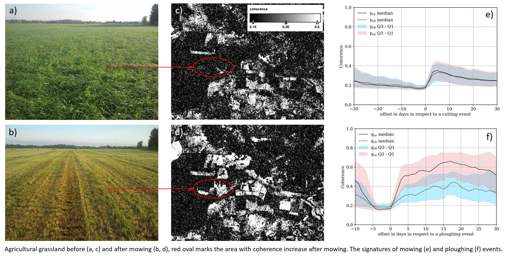
The study was carried out in Estonia, Northern Europe (between 57.5°N, 21.5°E and 59.8°N, 28.2°E). The study area is relatively flat with no steep slopes and altitudes ranging between 0 and 200 m above sea level (asl). Data about events were collected directly from the farmers and consisted of information about the start and end date of the activity and the area covered. In total, data about 1695 mowing and 195 ploughing events on 1159 and 177 unique agricultural parcels, respectively, were collected. The average area of mowing and ploughing events, respectively, is 10.4 and 12.2 ha, the minimum 0.6 and 0.9 ha, and the maximum 108.5 and 92.0 ha. Considering the main agricultural areas of the country (excluding forests and marshlands), events are geographically evenly distributed as seen in
Figure 1. The earliest reported mowing event occurred on 20 May, while the latest on 12 October 2017. In the case of ploughing, the earliest event was recorded on 1 July and the latest on 8 September 2017. The dataset covers majority of the agricultural season in Estonia, where green vegetation emerges in the beginning of May and lasts until October. The dataset includes also information about the main soil type (peat or mineral soil).
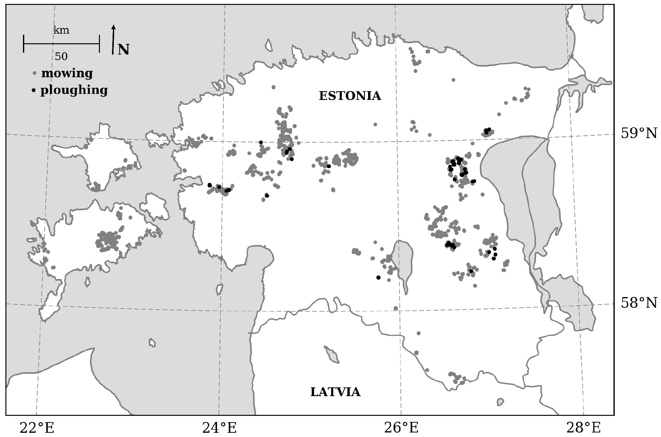
Agricultural grasslands on mineral soils are major ecosystems, but some less intensively managed grassland parcels are also in wetlands on peat-soils. Main grass species are from Poaceae (e.g., reed canary grass and timothy) and Fabaceae (e.g., clover and alfalfa) families. There are parcels with pure species and also the mixtures of them. The fields are cultivated in spring or late autumn and mown one to three times per season. In most of the fields the grass is collected and used as animal fodder. Some parcels are also grazed, which is less common than mowing.
Figure 2 presents typical Estonian Poaceae and Fabaceae agricultural grassland parcels before and after mowing. Parcels with Poaceae reed-like grasses have dominantly vertical structures. Parcels with Fabaceae clover-type grasses have also vertical structures from the stems, but the orientation of the canopy is more random.
2.2. Sentinel-1 Data
In total, 386 S1A/B SLC IW products acquired between 1 May and 30 October 2017, were processed. Local time of overpass was around 18:00 (15:00 GMT). A total of 87 products were from relative orbit number (RON)160, 62 from RON131, 84 from RON87, 93 from RON58, and 60 from RON29. These were organised into S1A/S1B 6-day pairs. Only nine products in the given time period were missing from the Copernicus Open Access Hub, slightly decreasing the data density for RON160 and RON87.
Besides different viewing geometries, the value of using multiple RONs is a shifted grid with independent temporal sampling. It should increase robustness to disturbances that are corrupting a single RON. The value of using multi-RON data is discussed in
Section 3.3 below.
Incidence angles range between 29° and 46°. Spatial resolution ranges between 2.7 and 3.5 m in slant range, but is fixed at 22 m in azimuth.
2.3. Sentinel-2 Data
In total, 351 Sentinel-2A and -2B L2A products acquired between 1 May and 30 October 2017, were processed. Local time of overpass was around 13:00 (10:00 GMT). Each Sentinel-2 image is a maximum of three days off from the closest Sentinel-1 image. A total of 14 products were from RON22, 74 from RON36, 67 from RON79, 50 from RON93, 78 from RON122 and 68 from RON136. As the focus was on Sentinel-1 coherence analysis, only the NDVI [
19], computed according to Equation (
1), was derived from Sentinel-2 to have a comparison with a well-known optical vegetation remote sensing parameter.
where band8 is the 8th band (near infrared with central wavelength of 842 nm) and band4 is the 4th band (red with central wavelength of 665 nm) of Sentinel-2.
2.4. Ancillary Data
Weather and precipitation data were derived from Estonian Weather Service database. The weather information is collected from a network of weather stations over Estiona, which form a sufficiently dense grid, so that to every location in our field database, a weather station not farther than 40 km can be found. The database includes observation history for many years and is publicly available at Estonian Weather Service homepage [
20].
2.5. Methods
The goal of data analysis was to characterize temporal changes in Sentinel-1 interferometric coherence caused by mowing and ploughing events on the fields and relate it also to the changes in optical images. For this, coherence time series were calculated about every field in the database in relation to the event. Average coherence of a field, imaging geometry parameters, imaging time and average NDVI was stored in a database. Analysis of the database of coherence values with different temporal distance from a farming event allowed to extract the typical behaviour by means of statistical analysis. The behaviour of Sentinel-2 NDVI was analysed in a similar way. The database formation process involved preprocessing a large amount of satellite images where average coherence and NDVI value was calculated for every parcel for every available date (constrained by image availability and cloud cover).
The Sentinel Application Platform (SNAP) toolbox was used for processing. The following steps were applied: apply orbit file, back-geocoding (using Shuttle Radar Topography Mission (SRTM) data), coherence calculation, deburst, terrain correction, and reprojection to the local projection (EPSG:3301). In the last step, data were resampled to 4 m resolution to maintain the maximum spatial resolution, and having square-shaped pixels. The terrain around the study areas is relatively flat, resulting in negligible topographic distortions of the SAR data. Coherence was calculated for each swath separately. Only pixels that were completely inside the parcel boundaries (also considering the averaging window used for coherence calculation) were used for calculation of results and to discard any interference beyond parcel borders. Coherence was computed pair-wise with 6-day time steps. For every coherence computation there was a new master and slave. The results were stored in a database following a forward-looking convention—coherence about date X means the coherence between Sentinel-1 images from date X and X + 6 days.
To understand how coherence (
) varies in relation to mowing and ploughing events,
from all parcels with recorded events were aggregated. All time series were shifted to the same grid with a step of one day by placing the event at time 0. The grid extends from
(i.e., 30 days before an event) to
(
Figure 3). The median value and third and first quartiles were calculated for each grid point. Ploughing signatures are presented in limited −10 to +30 day range, as the status of a grassland before a ploughing event was too variable for a meaningful generalisation.
2.6. Interferometric Coherence and Temporal Decorrelation
The amplitude of the complex correlation coefficient also known as coherence is calculated for two complex SAR acquisitions
and
, as
Estimated coherence
is a product of several terms specific to the measurement system, data processing steps and the targets that were imaged. It can be modelled as follows:
where
refers to temporal decorrelation,
to decorrelation due to signal-to-noise ratio, and
to other terms that may be present but are negligible in our case [
21].
According to [
4,
22,
23],
can be expressed, as
where
t is the temporal baseline between acquisitions,
is the radar wavelength, and
is the mean motion of scatters in the line of sight (LOS).
is a measure of change over time, it approaches 1 in the case as
approaches 0.
In the case of management of agricultural grasslands, there are three distinct phases that we need to evaluate in relation to : growth, mowing or ploughing event, and developed state. Growth occurs in the early vegetation season and after events. Developed state occurs between the previous states when vegetation is steady and relatively tall.
Movement and growth of vegetation in the LOS causes temporal decorrelation. Coherence is also decreased due to variations in the moisture content of soil and vegetation, which affects scattering centre location, as seen by SAR. During the growth phase, physical and moisture changes are gradual. Changes accumulate as more vegetation is visible in the LOS, causing decorrelation. Coherence would remain low throughout the developed phase.
Removal of vegetation during a mowing event acts in two ways in relation to . The actual event drastically changes the scatterers. calculated for an image pair where the event occurred between the acquisitions would be very low. Depending on the canopy cover, it can be even lower than the coherence of the developed state. For image pairs after the actual event, would be higher when compared to pairs where vegetation was present—as the vegetation is removed, returns from more coherent soil increase.
A similar behaviour applies to ploughing. The event itself causes decorrelation, and conditions after it would cause higher . Total lack of vegetation would suggest even higher values than in the case of mowing.
Precipitation is a source of decorrelation. Variations of relative permittivity in the resolution cell between acquisitions cause coherence to decrease, as scattering centre changes according to permittivity change. The variations are hard to predict as one must consider a multitude of factors, including air temperature, wind, soil and vegetation conditions.
The estimated
is also a function of Equivalent Number of Looks (ENL) defined by the size of the averaging window in (
2) [
24]. Contrast between areas of low coherence will be lost if a small averaging window (resulting in low ENL) is used in (
2) [
25]. We used an averaging window ensuring a square footprint on the ground (approximately 70 × 70 m) and an ENL value between 40 and 50, depending on the swath. According to [
24,
26], ENL of 45 would ensure contrast for
values larger than 0.13. Correction for
term in (
2) was applied according to [
27].
3. Results
3.1. Aggregated Time Series
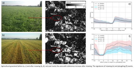
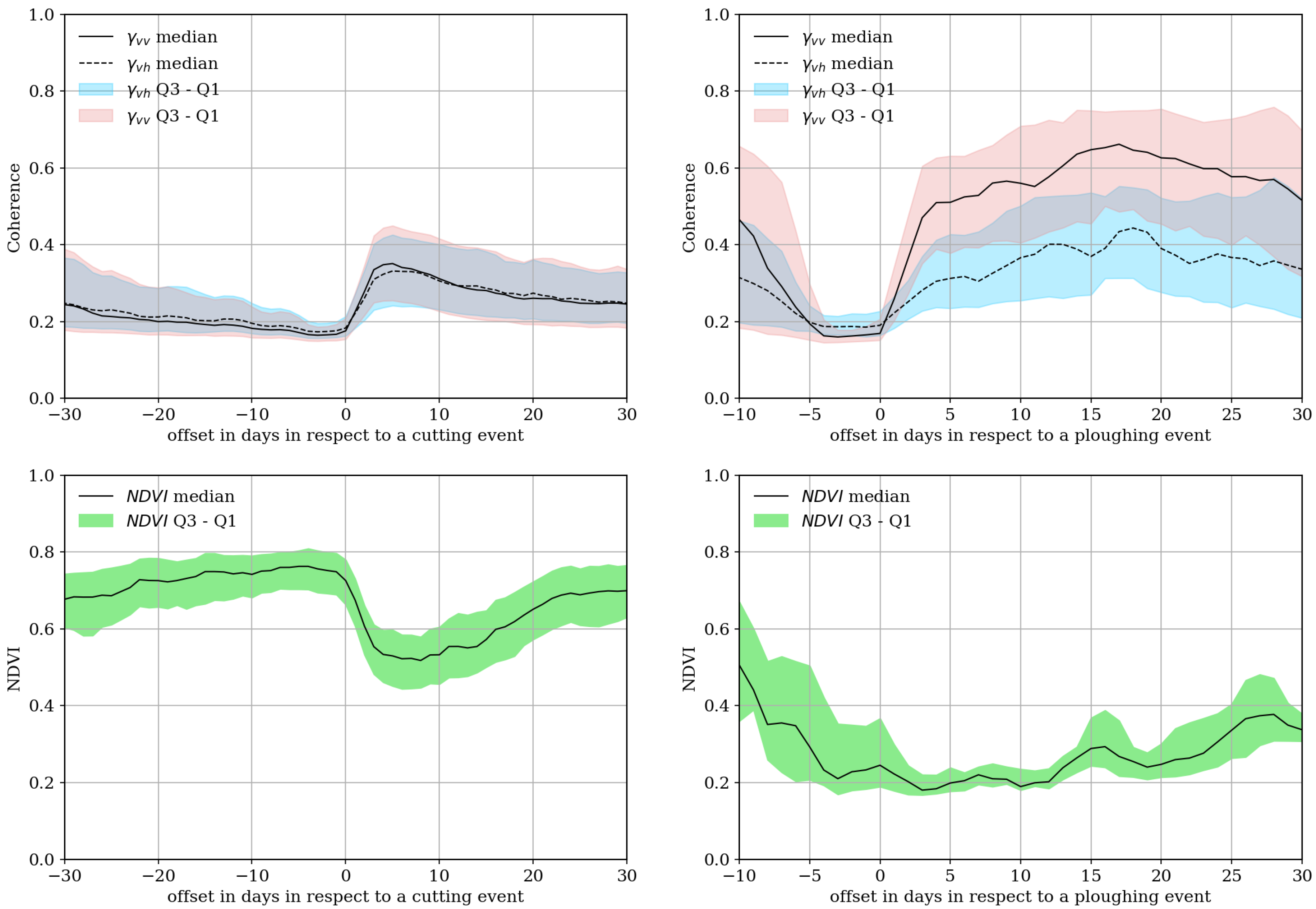
and
signatures of mowing and ploughing events together with the respective NDVI curves, smoothed with a 3-day averaging window (to reduce the noise), are presented in
Figure 3. Understanding the signatures of the farming events are important for adapting satellite monitoring for CAP subsidy checks [
28], where the signatures are called ‘markers’.
In the case of mowing,
decreases slightly but gradually before the event reaching a minimum value just before it. After the event,
reaches a maximum after which it starts to decrease gradually again. Signatures for both
and
follow each other very closely suggesting invariance to polarisation. Mowing signature is smoother due to more data points (1695 mowing vs 195 ploughing events). Additional variability in ploughing signature is due to other management practices taking place around the time of a ploughing event. Ploughing is often performed closely after mowing and other events—such as seeding or cultivation—might follow. This proximity introduces the large variability evident in
Figure 3.
In general, the coherence signature of ploughing is similar to that of mowing. A minimum value is reached just before the event followed by a maximum after it. The maximum, however, occurs much later, between 10 and 20 days after the event.
The NDVI signature of mowing follows the coherence signature inversely. While the mowing event causes coherence to increase from 0.18 to around 0.35, NDVI decreases from 0.75 to 0.5. The NDVI signature of ploughing is less clear. From 0 to 12 days after ploughing NDVI is relatively stable at 0.2, but after that the growth of it has larger variability.
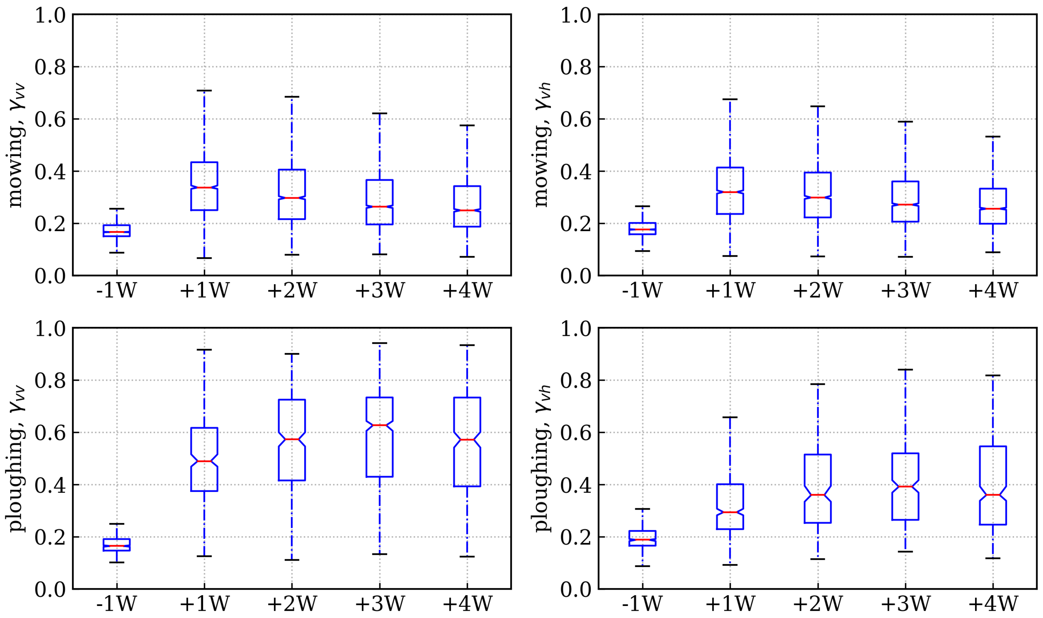
To better understand the dynamics of
around mowing and ploughing events, coherence values were divided into five time groups. The first group contains measurements where the first acquisition in the interferometric pair was acquired seven to one days before an event and it is labelled as −1 W. The second group labelled as +1 W corresponds to values from up to one week after an event, i.e., acquisition occurred one to seven days after the event, etc. Measurements that were taken on the same day as the event were discarded as the exact time of the activity was not known. Boxplots of these time groups are shown in
Figure 4 and the median values are presented in
Table 1.
In the case of mowing, the highest median value is for +1 W group (0.34) with the increase from −1 W being 0.17. , on the other hand, increases by 0.14, from 0.18 at −1 W to 0.32 at +1 W. On average, exhibits the largest increase between −1 W and the maximum post-event median. In the following weeks, the difference between and continue to be in the range of 0.02 units.
As discussed before, differences between polarisations are larger in the case of ploughing. increases between −1 W and +1 W by 0.33 and by 0.10. For both polarisations maximum is reached at +3 W being 0.63 for VV and 0.39 for VH polarisation.
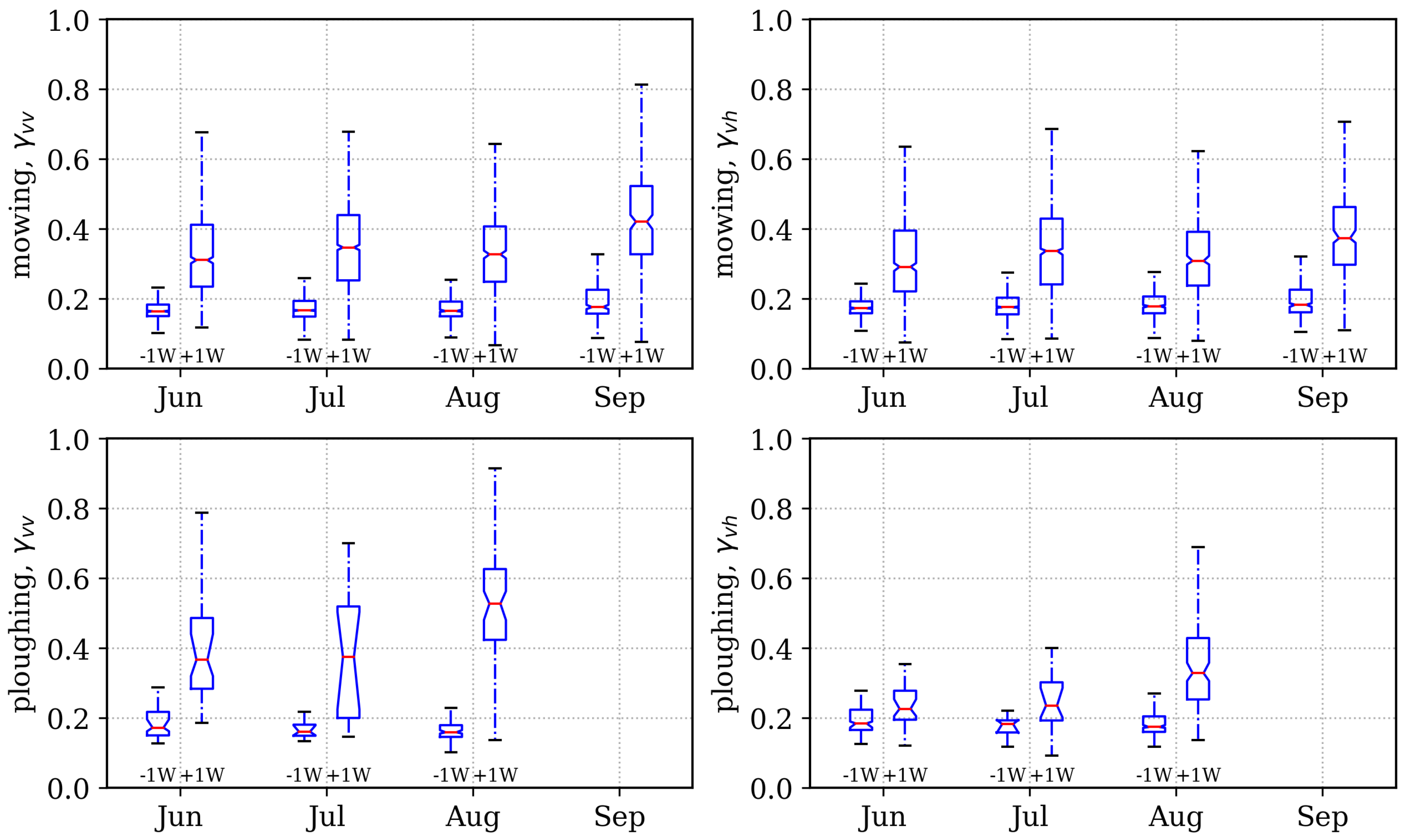
Growth of vegetation varies depending on the time of the year. To see whether it influences results of this study we further divided the −1 W and +1 W groups into subgroups depending on the month when the event occurred.
Figure 5 and
Table 2 contain the results. Results are presented only for months when there were enough events.
For both event types and polarisations, −1 W values stay stable for most of the season, being between 0.16 and 0.18. +1 W values vary more. In the case of mowing, median values increase from 0.31 in June to 0.35 in July, decrease temporarily to 0.33 in August and reach the maximum at 0.42 in September. medians follow the same pattern with slightly different absolute values.
In the case of ploughing, the difference between +1 W in June and August is 0.16. The biggest difference in the case of is also between June and August—0.10. Higher variability in the case of ploughing is likely due to fewer events. Also, vegetation generally allows to maintain more steady levels of moisture on the parcel, and total lack of it after ploughing would lead to higher sensitivity to moisture changes.
3.2. Relation of Sentinel-1 Coherence to Sentinel-2 NDVI
Figure 6 presents a series of Sentinel-1 backscatter and coherence and Sentinel-2 natural colours and NDVI subsets about a grassland area of Western Estonia. It provides a visual comparison of the traces of mowing events on Copernicus satellite imagery derivatives.
Due to cloud cover and data availability it was not possible to get the Sentinel-1 and -2 images about the exact same dates. Yet the time series gives a good example about the dynamic range of Sentinel-1 coherence and Sentinel-2 NDVI of different mown and unmown grassland parcels. Before mowing the NDVI of tall grass can be above 0.8, whereas after mowing it will fall around 0.4 (
Figure 6g,h). Freshly mown areas seem to be well visible also on Sentinel-2 natural colours RGB (
Figure 6e,f).
In Sentinel-1 coherence (
Figure 6c,d) the pre-event tall grass values are close to the noise floor at 0.15, whereas after mowing it can reach to 0.5 and sometimes even higher.
Figure 6 illustrates very well also the value of interferometric processing of Sentinel-1 data. An area mown between 19 and 25 July is indicated with a red oval. Notice that on backscatter image there is almost no difference—grassland backscattering remains low no matter the grass height and the mowing status (
Figure 6a,b). While the coherence image is not visually appealing, it contains the information and freshly mown areas are well visible as the bright high coherence areas (
Figure 6d).
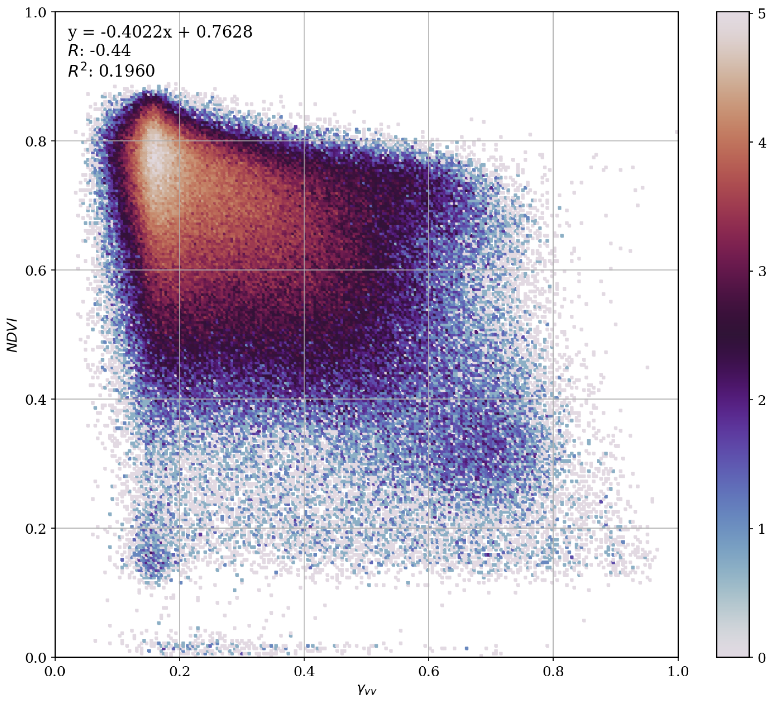
To explore better the relation between Sentinel-1 coherence and Sentinel-2 NDVI a scatterplot was compiled. Only such X-Y pairs were included where the Sentinel-1 VV-coherence and Sentinel-2 NDVI was available about the very same date of a given grassland parcel. The result is shown in
Figure 7.
It is well visible that there is no strong direct correlation (
Figure 7), because they measure different physical parameters. Exact Sentinel-1 coherence and Sentinel-2 NDVI values depend on multiple factors. NDVI is mainly sensitive to the green, chlorophyll containing biomass, whereas interferometric coherence is a normalised measure of change between two complex radar images, which in turn in natural conditions are mainly sensitive to water and objects containing water. Yet, the tendency is clear—high coherence corresponds to low NDVI and vice versa. The small cluster in the bottom left (low coherence and low NDVI) corresponds most probably to the parcels, which had low and sparse vegetation, but the coherence is low due to rainfall happening right before either of the InSAR pair images.
3.3. Instructive Individual Time Series
Whereas the general behaviour of Sentinel-1 repeat pass coherence is intuitive to understand—short and sparse vegetation corresponds to high coherence, tall and dense vegetation to low coherence—there are still some details to be considered for correct coherence time series interpretation.
Below, the time series of three instructive parcels are given to illustrate the dynamics of coherence on typical Estonian grasslands.
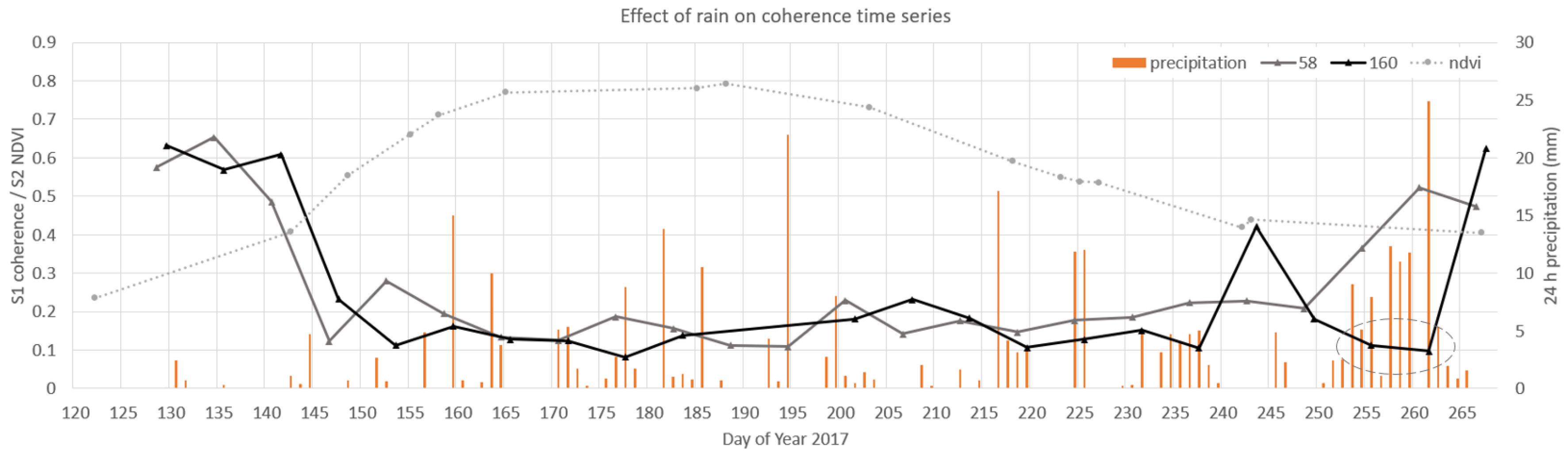
Figure 8 presents an unmown grassland parcel affected by heavy rain.
Figure 9 corresponds to a grassland growing on a wet marshy soil and
Figure 10 a parcel, which was first mown and then ploughed. The rain, marshland and ploughing effects illustrated below were common in the 2017 dataset used for the study. Understanding them will help to design better monitoring systems for grasslands as well as other agricultural applications exploiting Sentinel-1 coherence time series.
Figure 8 shows the S1 coherence and S2 NDVI time series of a typical unmown grassland. NDVI has a relatively smooth arc like curve being maximum at mid summer and decreasing slowly in the second half of the summer as the senescence of vegetation occurs. The behaviour of coherence is inverse to NDVI—being high in the early and late season and low in the middle.
It is important to notice the effect of rainfall on the time series. The average accumulated past 6 hours precipitation prior to the Sentinel-1 data take on DOY 262 at 15:57 UTC in the nearby Türi, Pajusi and Viljandi weather stations was 22 mm [
20]. By DOY 262 due to senescence the vegetation was already drier and sparser resulting in coherence increase as one can see from RON 58 data points. Still, two consecutive RON 160 coherence data points (DOY 256 and 262) are pushed down close to the noise floor leaving the RON 58 time series unaffected. This is a major difference with the effect of farming events as explained in
Figure 10 below.
Daily 24 h precipitation sums (accumulated at 18:00 UTC) are also given in
Figure 8. Again they are the averages of the closest nearby weather stations from Türi, Pajusi and Viljandi [
20], which are not further than 40 km from the particular grassland parcel. One can see that high precipitation values on the same day with the Sentinel-1 acquisition tend to result in low coherence of two consecutive coherence values of a single RON. Precipitation between the InSAR pair acquisitions often do not alter the coherence, as the field can quickly dry out depending on the weather.
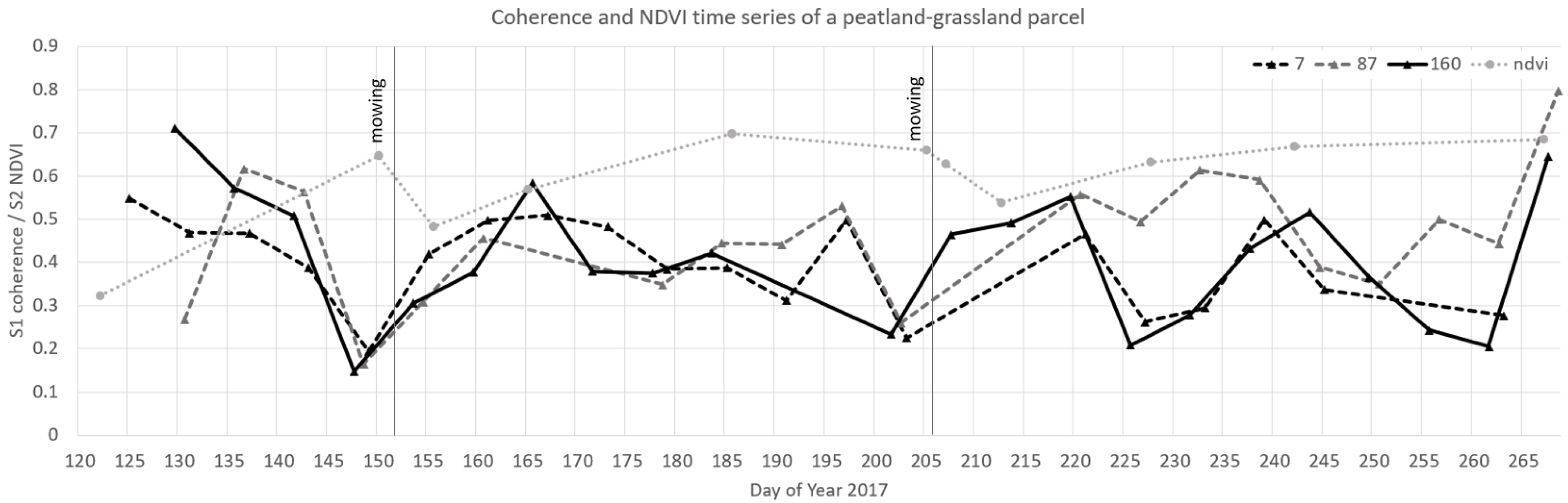
Figure 9 presents the S1 VV-coherence and S2 NDVI time series of a typical grassland on a wet peat-soil (e.g., close to peat extraction areas or river valleys). The coherence for the unmown tall grass state is higher-around 0.4 to 0.5, whereas for drier mineral-soils it is below 0.2. NDVI is also slightly lower—never exceeding 0.7, whereas for mineral-soil grasslands it can be over 0.8 in the case of unmown grass. Another property typical for the peat-soil grassland is a general instability of the coherence; even without any farming events, the coherence can fluctuate by 0.2 or more.
The signature of the mowing events on peat-soils is different. Whereas on mineral-soils the mowing event is indicated by the transition of coherence from low to high, it is different on peat-soils. The general coherence levels before and after the mowing event seem virtually unchanged, the only characteristic is a temporary decrease of coherence just before the mowing event to 0.15–0.25 (taking into account that here the coherence at date X presents the coherence between images of date X and date X + 6 days). It is important to notice that all of the RONs are affected and only the interferometric pairs, where the mowing event took place in-between, as it totally changed the vegetation structure.
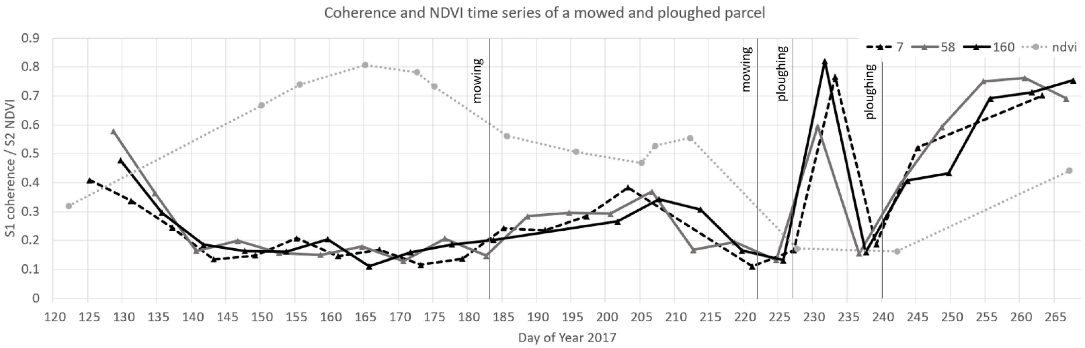
Figure 10 shows S1 VV-coherence and S2 NDVI time series of a grassland on mineral-soil, which was first mown on DOY 183 and a second time on DOY 222. After the second mowing the parcel was also ploughed twice (on DOYs 227 and 240). The first mowing increased the coherence from below 0.2 close to 0.3, where NDVI decreased from 0.73 to 0.57 at the same time. After the second mowing the coherence increase and the NDVI decrease is almost undetected as it is followed by ploughing just five days after the mowing event. Yet the two ploughing events have very distinct signatures of the coherence time series. The coherence is very low (close to the noise floor) just before the ploughing event and much higher afterwards. It is important to notice how the farming event affects a single data point in all of the RONs—a remarkable difference compared to how rain is affecting coherence, which is decreasing the coherence for two consecutive coherence data points of just a single RON.
4. Discussion
In the following section, possible reasons behind the observed behaviour in the Results part is discussed. In case, available references to the previous studies are given.
Observed coherence behaviour respect to mowing and ploughing events (
Figure 3) is in general well in line with the theory in
Section 2.6. There is still a detail to be noticed - maximum coherence occurs with a delay. If some vegetation was left on the parcel after mowing it would take some time for it to dry out and stop interacting with the SAR signal. Similar behaviour is reported in a study with Sentinel-2 optical data. When the grass was mown but not removed, the NDVI was still relatively high, it decreased to even lower levels in time when the vegetation was removed or it dried out [
29].
The coherence maximum is even more delayed for ploughing events. This might be due to several reasons. Overturned soil with no vegetation cover tends to dry out. Moisture levels change between acquisitions causing decorrelation. After they reach a stable level, coherence can increase. Also, possible follow-up activities such as seeding and fertilisation cause decorrelation, and coherence increases only after all activities cease. Maximum value is reached when the soil has dried to a stable moisture level and hence also the scattering patterns between the six-day interferometric pair change less.
Another dissimilarity between mowing and ploughing is the difference due to polarisation. values are remarkably higher than after the ploughing event. This is most probably due to the structure of the overturned soil that favours VV backscatter. This should be considered when designing algorithms for classification of management practices. For both event types coherence values reach a minimum just before the actual event. When an event happens between acquisitions, coherence for the affected pair is the lowest due to profound changes in the soil and vegetation caused by mowing or ploughing.
Out of the signatures presented in
Figure 3, the NDVI behaviour respect to ploughing event was the least clear. The variability evident 12-30 days after a ploughing event could be caused by different grass species different growth tempo and possible follow-up farming activities such as seeding. Even more variable is the NDVI just before the ploughing event. While for mowing it is very stable high NDVI (as only tall well-developed grassland is usually mown), the parcel status before a ploughing event can be very different: spring-time ploughing of an almost bare field, ploughing after mowing, second ploughing event right after the first one, etc.
VV- and VH-coherence follow generally the same trend, but the behaviour is not exactly one to one. On the level of the individual parcel, the differences can be even larger than on the aggregated plots (
Figure 3,
Figure 4 and
Figure 5) and are related to structural differences of vegetation (primarily vertically oriented stems and leaves or more randomly oriented canopy) [
30]. In case of soil scattering,
is not polarisation dependent considering the moisture component [
31]. We must consider that mowing does not completely remove vegetation from a parcel. Unfortunately we do not have information about vegetation height in parcels used in this study. Yet from the previous studies about Estonian grasslands we know that unmown tall grass ranged typically between 50–75 cm and mown short grass between 5–30 cm. Wet biomass ranged from 0.1 (mown grasslands) to 4.5 (unmown tall grass) kg/m
[
32,
33]. It is very likely that similar characteristics were also present during 2017.
Pre-event values of
and
are very stable and are largely determined by ENL used in coherence computation [
34], as described in
Section 2.6. For the −1 W group, events occurring between the acquisitions cause total decorrelation. The ’noise floor’ due to ENL in our case is 0.13, i.e., coherence cannot be lower than that.
We mentioned in
Section 2.2 that there were nine S1 products missing for RON160 and RON87 for a period between 1 May and 30 October. It has negligible influence on the results presented in
Figure 3 and
Figure 4. However, on a parcel level, lack of S1 acquisitions may be problematic. If a single acquisition is missing, it influences two pairs of acquisitions and a period of 12 days, creating a gap of 18 days between usable coherence values. The severity of this varies depending on the latitude and regional data acquisition plan that influences the data density [
35]. It is possible that a single missing acquisition may cause an event to have no visible effect on
time series. Using multi-RON data can help to solve this challenge as described in the paragraph below.
Whereas a farming event affects a single coherence data point of all the RONs, causing it to be very low for interferometric pairs, where the farming event took place in-between, rainfall caused coherence loss is image and RON specific. It affects just a single RON and leaves other RON coherences unaffected. A significant rainfall just before an SAR image acquisition totally alters the scattering properties of the respective image [
36]. As the image is part of two consecutive interferometric pairs (first time when the one is the after image and the second time when the one is the before image)—two consecutive coherences of a certain RON will be temporarily lowered. This underlines the value of using multiple RONs for operational agricultural applications as it helps to solve the ambiguity between rainfall and farming events on coherence time series. The advantage of using multiple RONs is mainly in the shifted temporal sampling and not so much in the different viewing geometries. Rainfall right before a Sentinel-1 data take can mask the traces of a farming event in the time series of a single RON, but (if available) on the other RONs the traces are still visible.
Figure 8 presented also the 24 h accumulated precipitation data, allowing to compare the rainfall info with coherence time series. Care must still be taken when interpreting it. During mid-season (DOY 150–230) due to tall well-developed vegetation the coherence was already very low and the precipitation effects are therefore not so pronounced for this period. The resolution of the given precipitation data from the Estonian Weather Service is 24 h, most of the rainfall could have been many hours before the Sentinel-1 data take (around 15:00 UTC) and by that time the fields could have already been dried out. Studying precipitation effects on Sentinel-1 coherence was not the main focus of our research. For the readers interested in this topic it is recommended to select short grass low biomass grassland parcels as close as possible to the weather stations. There, the dynamics of coherence due to precipitation should come out in the most pure and clear way.
The fluctuating coherence levels of the grassland parcel on peat-soil are likely connected with the moisture changes in the soil and vegetation. This is altering the scattering properties and as a result also the coherence. High Sentinel-1 coherence on peatland vegetation is also reported in [
37], which discusses in detail the relation between the coherence and water regime.
5. Conclusions
According to the study, mowing and ploughing can be detected from Sentinel-1 coherence time series with high confidence. We demonstrate it based on a large ground reference data set covering 1695 mowing and 195 ploughing events on agricultural grassland in Estonia. While the vegetation is present, the values are close to the noise floor. For both event types, coherence tends to increase after an event as scattering from the soil becomes dominant. As the vegetation regrows, coherence slowly decreases to pre-event values. On average, ploughing causes a larger increase, at least for VV polarisation. In the case of mowing, both polarisations exhibit very similar behaviour to each other. The magnitude of increase varies depending not only on the event type but also on vegetation species and specific management practices within one event type.
We discussed the effect of rainfall and farming events on Sentinel-1 coherence time series and explained the means to distinguish them using the time series of alternative viewing geometries and independent temporal sampling (different RONs). We also compared how the coherence time series for grassland on mineral soil differ from the one on peat-soil.
Precipitation right before a Sentinel-1 image acquisition can suppress coherence, masking the increase due to event and hiding the signature of mowing or ploughing. For reliable operational applications, a dense multi-RON time series should be used for the analysis to reduce the effect of precipitation caused disturbances.
The results presented here show the traces of mowing and ploughing events on Sentinel-1 coherence time series convincingly. However, the detection limits are not fully understood. Future studies should compare the coherence values with in situ grass height and wet biomass measurements. This could help to find how much remainder biomass could be left on ground to leave the farming event still visible on Sentinel-1 coherence time series and possibly contribute towards a grassland biomass retrieval algorithm based on Sentinel-1 and other data sources.

 ,
, 


