First Evidences of Ionospheric Plasma Depletions Observations Using GNSS-R Data from CYGNSS


1
CommSensLab-UPC, Department of Signal Theory and Communications, UPC BarcelonaTech, c/Jordi Girona 1-3, 08034 Barcelona, Spain
2
Institut d’Estudis Espacials de Catalunya-IEEC/CTE-UPC, Gran Capità, 2-4, Edifici Nexus, Despatx 201, 08034 Barcelona, Spain
*
Author to whom correspondence should be addressed.
Remote Sens. 2020, 12(22), 3782; https://0-doi-org.brum.beds.ac.uk/10.3390/rs12223782
Submission received: 10 October 2020
/
Revised: 13 November 2020
/
Accepted: 14 November 2020
/
Published: 18 November 2020
(This article belongs to the Special Issue Applications of GNSS Reflectometry for Earth Observation)
Abstract
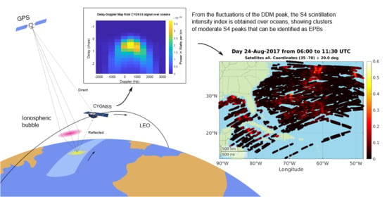
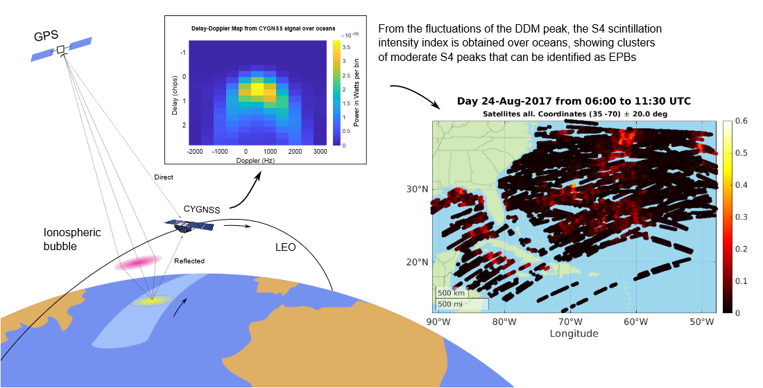
:At some frequencies, Earth’s ionosphere may significantly impact satellite communications, Global Navigation Satellite Systems (GNSS) positioning, and Earth Observation measurements. Due to the temporal and spatial variations in the Total Electron Content (TEC) and the ionosphere dynamics (i.e., fluctuations in the electron content density), electromagnetic waves suffer from signal delay, polarization change (i.e., Faraday rotation), direction of arrival, and fluctuations in signal intensity and phase (i.e., scintillation). Although there are previous studies proposing GNSS Reflectometry (GNSS-R) to study the ionospheric scintillation using, for example TechDemoSat-1, the amount of data is limited. In this study, data from NASA CYGNSS constellation have been used to explore a new source of data for ionospheric activity, and in particular, for travelling equatorial plasma depletions (EPBs). Using data from GNSS ground stations, previous studies detected and characterized their presence at equatorial latitudes. This work presents, for the first time to authors’ knowledge, the evidence of ionospheric bubbles detection in ocean regions using GNSS-R data, where there are no ground stations available. The results of the study show that bubbles can be detected and, in addition to measure their dimensions and duration, the increased intensity scintillation () occurring in the bubbles can be estimated. The bubbles detected here reached values of around 0.3–0.4 lasting for some seconds to few minutes. Furthermore, a comparison with data from ESA Swarm mission is presented, showing certain correlation in regions where there is peaks detected by CYGNSS and fluctuations in the plasma density as measured by Swarm.
1. Introduction
1.1. Physics of the Ionosphere
The ionosphere is a layer of the atmosphere that plays a very important role in satellite communications and Earth Observation. This layer, which ranges from around 60 km to more than 500 km altitude, contains free electrons and ions, making a sort of “electric conductor” that interacts with the electromagnetic waves crossing it.
The shape and density in electron density profile, are highly affected by many factors in a balance between production and destruction processes driven, mainly, by solar irradiation. Also, its dynamics is influenced by the movements of the inner atmospheric layers and the outer magnetosphere. Because of all these factors, the ionospheric fluctuations take place in a wide range of amplitudes and duration, from kilometers to several meters and from a few seconds or minutes to days.
It has been observed that there is an increase in the activity, related to solar irradiation, in the transitions (sunrise and sunset), with a rearrangement of the layers. Seasonal dependence is also noticed, with more activity during the periods around the Spring and Autumn Equinoxes. And, on top of that, there is a positive correlation with solar activity following the 11-year solar cycle, with a minimum happening this year 2020.
Electromagnetic waves crossing the ionosphere may suffer from those perturbations, making the signal to change its direction of propagation, polarization, or creating fluctuations in intensity and phase, the so-called, ionospheric scintillation. This phenomenon is known since the first satellites put in orbit and it has been a subject of study until today. Some models have been developed to try to describe and predict its behavior. During the past years, some ionospheric scintillation models have appeared, for example:
- The Global Ionospheric Scintillation propagation Model (GISM) [1] provides time series of intensity and phase scintillation models using a turbulent ionosphere, and an electromagnetic waves propagator in turbulent media, using the Multiple Phase Screen theory (MPS) [2]. GISM is the model accepted by the ITU-R (International Telecommunication Union - Radiocommunication Sector) for the ionospheric communications [3].
- The WideBand MODel (WBMOD) [4] is also based on electron-density irregularities and uses the MPS theory to compute the scintillation effects in an statistical sense. In this model it is possible to set-up a communication scenario (time, location, and other geophysical conditions).
- The Wernik-Alfonsi-Materassi Model (WAM) [5] also uses the MPS theory, but generates its statistics from in situ measurements on ionization fluctuations measured by the Dynamics Explorer 2 satellite. It can also predict the ionospheric index along a defined path given some environmental conditions.
More recently, in the context of a European Space Agency (ESA) project, the GISM functionalities were extended in the UPC/OE/RDA (Universitat Politecnica de Catalunya/Observatori de l’Ebre/Research and Development in Aerospace) SCIONAV model [6], to reproduce more realistically the behavior of ionospheric scintillation at both low and high latitudes, taking into account the different physical phenomena that create them, such as the bubbles and depletions in equatorial regions and it is based on lookup tables resulting from extensive analyses.
However, all these models require further improvements:
- In polar and auroral regions the models still need a better description in terms of velocity, distribution, duration and intensity of the ionospheric effects.
- A better modelling (3D) of the equatorial plasma bubbles (EPBs) can be incorporated in the UPC/OE/RDA SCIONAV model, relating its 3D properties to the altitude, and the amount of plasma depletion with the produced [7].
- In GNSS-R applications, some anomalous fluctuations have been reported in equatorial regions in regions over calm ocean, which are supposed to come from ionospheric scintillation [8].
1.2. Using GNSS-R to Study the Ionosphere
The goal of this study is to provide a way to improve the ionospheric models, by means of GNSS-R. This idea was firstly proposed in 1996 by S. J. Katzberg and J. L. Garrison [9], but not really explored the following years because the reflection over ocean (rough) surfaces is mostly incoherent, and sensitive to the winds, as reported in an airborne experiment of the same authors [10]. It was not until 2016 that it was shown [8] that the large fluctuations in the peak of the measured Delay-Doppler Map of GNSS-R instruments around the geomagnetic equator in calm sea conditions (wind speeds < 3 m/s), where reflections are more coherent, could be due to ionospheric scintillation.
The main purpose of GNSS-R missions is to study geophysical parameters of the Earth by studying the reflection of GNSS signals on the Earth’s surface. Applications include sea altimetry, soil moisture measurement or ice detection. The signals used to apply this technique cross the ionosphere in their down-welling and up-welling paths, that is, first from the GNSS satellite to the specular reflection point on the Earth’s surface, and then from this point to the GNSS-R receiver. Because of the height of the satellites involved, the down-welling path always crosses all the ionospheric layers, but the up-welling one may only cross some of them, depending on the altitude of the GNSS-R instrument.
Furthermore, GNSS signals would only allow the study of ionospheric scintillation in the GNSS bands, usually the L1/E1/B1, L2, and L5/E5. Other bands object of interest nowadays in Earth Observation, such as P-band (to be used in ESA BIOMASS Mission) are also affected by these perturbations, but they cannot be detected and/or quantified by this technique, although it could be applied using other signals of opportunity such as those from MUOS (Mobile User Objective System) satellites [11].
2. Materials and Methods
The current study uses open data from NASA CYGNSS (Cyclone Global Navigation Satellite System) mission [12,13], which continuously delivers GNSS-R data since March 2017. NASA CYGNSS is a microsatellite constellation led by the University of Michigan and the Southwest Research Institute, launched and operated by NASA in December 2016. The mission main goal is to provide a better forecast of hurricanes by studying the interaction between the sea and the atmosphere.
2.1. CYGNSS Dataset Description
The open-access CYGNSS database is provided by the Physical Oceanography Distributed Active Archive Center (PO.DAAC) [14]. The data is recorded continuously since 17 March 2017, for each of the 8 satellites in orbit. The data includes the DDM (Delay-Doppler Map), that is the cross-correlation of the reflected signal with a replica of the transmitted signal for different delay lags, and Doppler frequencies [15]. CYGNSS provides DDMs from up to the 4 channels tracking the signals received from 4 different GPS satellites, with a sample rate of 1 Hz. For each sample, auxiliary data such as the timestamp, the position of both CYGNSS satellite and the emitting GPS spacecraft are provided, together with the post-computed position of the specular point for the reflected signal on the Earth’s ellipsoid.
In any case, the data from reflections is only available from around 40N to 40S around the equator, as the satellite orbit inclination is around 35°. The orbital period is ∼95 min but, as the constellation is formed by 8 satellites distributed along the orbit, the overall revisit time is much less. Figure 1 shows the average number of samples measured during one day by the whole constellation as a function of the latitude per different cell sizes. CYGNSS has an almost circular Low Earth Orbit (LEO) at an altitude of ∼520 km, at an average speed of 7.6 km/s, much larger than the GPS satellites linear velocity (3.89 km/s), which complete an orbit every 12 h. Table 1 summarizes the mission parameters.
2.2. Data Processing
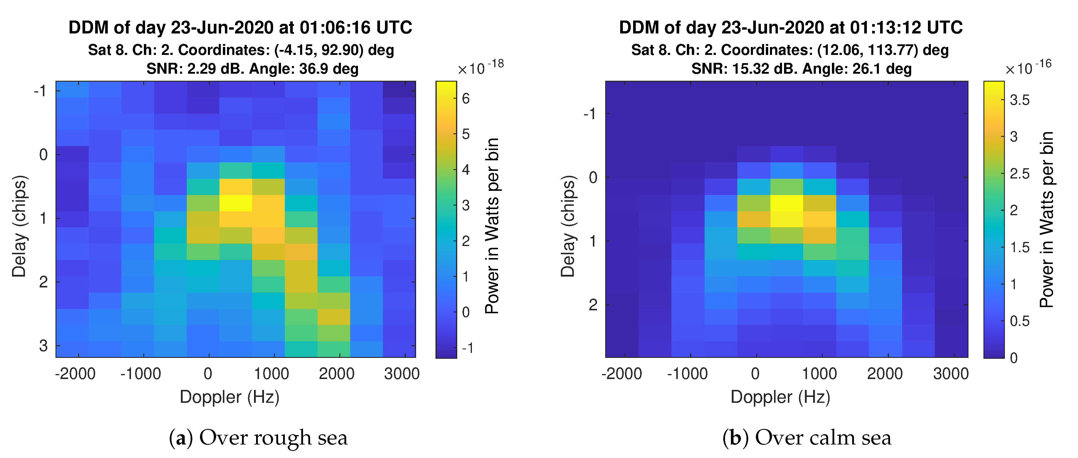
The data processing is performed to derive the CYGNSS observables of ionospheric activity. Source data comes from the DDMs. DDMs provided by CYGNSS has a size of 11 Doppler frequency bins × 17 delay bins, with a resolution of 200 Hz per Doppler bin, and 0.2552 chips delay bin. Since 1 C/A chip is equal to 1/1,023,000 s, it is equivalent to 293.3 m. Therefore, the resolution per delay bin is 74.8 m. The images below present two examples of CYGNSS’s DDM over two different surfaces.
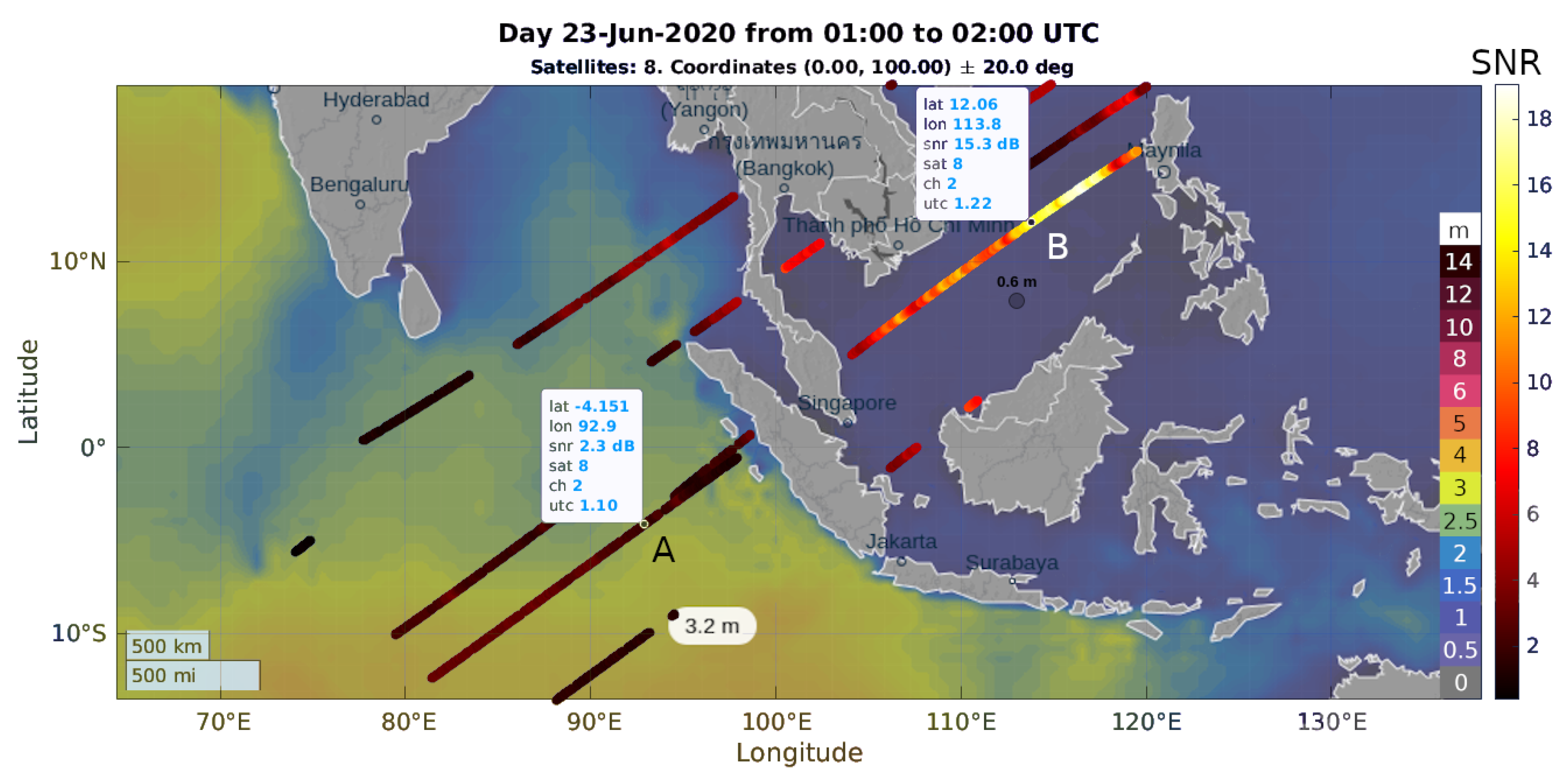
In order to assess the conditions of sea surface during the acquisition of these measurements, sea wave height is overlaid with the specular reflection points where the DDMs were taken, and it is shown for both cases in Figure 2, at points labeled as A and B. In the case of the DDM for rough water surface (Figure 3a) the SNR (Signal-to-Noise Ratio) is 2.3 dB and the wave height is around 3 m, marked in the map as A. For the calm ocean in Figure 3b, the SNR is much higher, around 15.3 dB, and the waves are around 0.6 m, marked as B in the map.
To perform this study, the main source of information is taken from the SNR (Signal-to-Noise Ratio) measurements available in the CYGNSS database. The SNR is post-computed on the ground using the DDM values as follows:
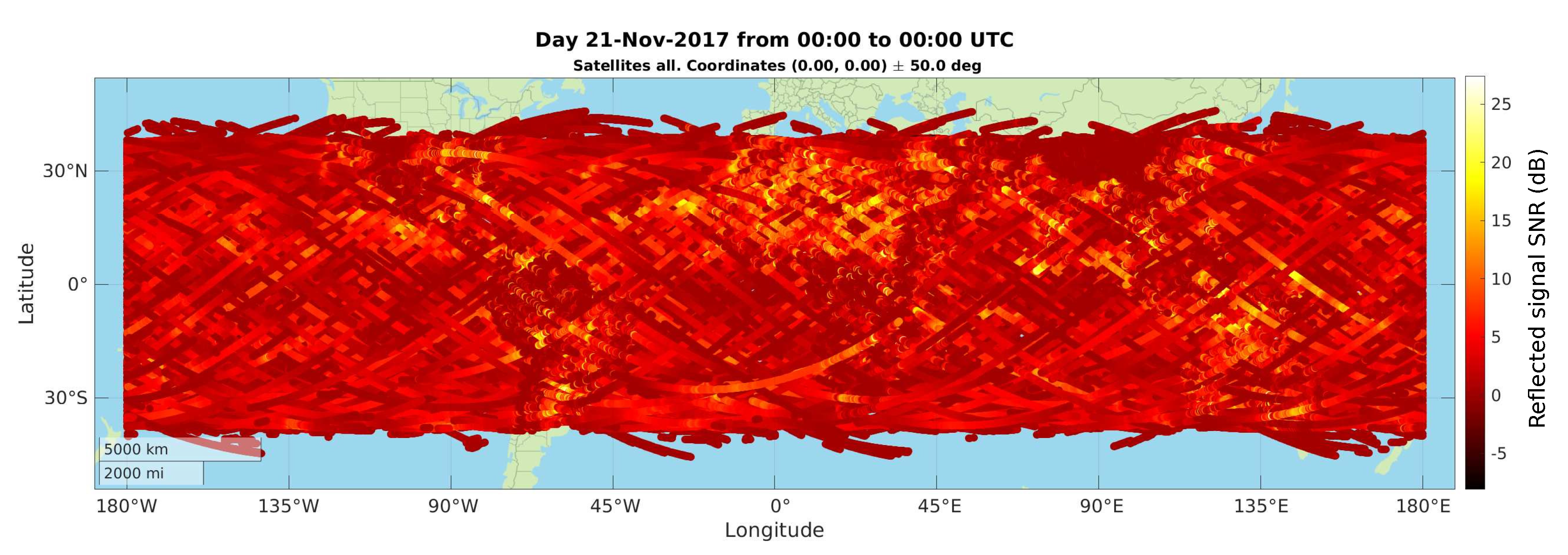
where , is the value of the DDM bin with maximum signal and is the average noise per bin, computed from the delay-Doppler bins before the DMM peak (i.e., delay < 0, as in Reference [8]. The value of the SNR is then given in decibels (dB). The maximum number of samples per day, considering the 8 satellites and their 4 channels, is around measurements. An example of this data is plotted in a world map in Figure 4, where both the measurement over land and oceans are displayed. Colorbar indicates the SNR of reflected signal in dB.
As the aim of the study is to observe the possible fluctuations in the intensity of the signal after crossing the ionosphere, the following computation is performed for every vector of data in a day. Having the 4 channels of SNR values during a whole day, it is chopped from a user-input “start_time” to an “end_time”. Then, using the quality flags that the CYGNSS database provides, the vector is chopped using only the points over the oceans farther away than 25 km from the coastline, and within a rectangular area that the user can define.
The output is a vector of data with internal discontinuities in time. In each per-channel vector, there are also discontinuities in the GPS satellite tracked. These discontinuities can be detected by the change of the PRN (Pseudo-Random Number) that identifies the tracked GNSS transmitter. Both types of jumps must be avoided in the computation of , because they may create false peaks. So, the vector, per each of the 4 channels, is divided into those periods between jumps (PRN or time jumps), and then the computation of the value is done using:
where I is intensity in linear units, computed from the SNR value in dB, and the average is computed using a 12-samples-moving window along the vector.
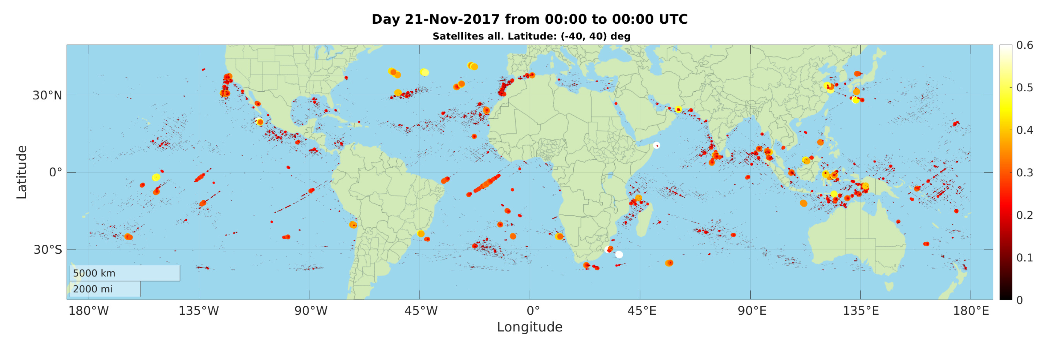
In Figure 5, the values using the SNR data from Figure 4 are plotted. For the sake of clarity in the interpretation, the points where is lower than 0.1 are not shown, and for the rest, their point size and color are proportional to the .
Additionally, the roughness of the water surface could make the reflection to be diffuse instead of specular. This would happen when there are high waves in the area, as opposed to having a flat ocean surface. In practice, this is making a sort of filter in which the possible scintillation happening over rough sea surfaces, is hidden, keeping only high values over regions with a calm ocean.
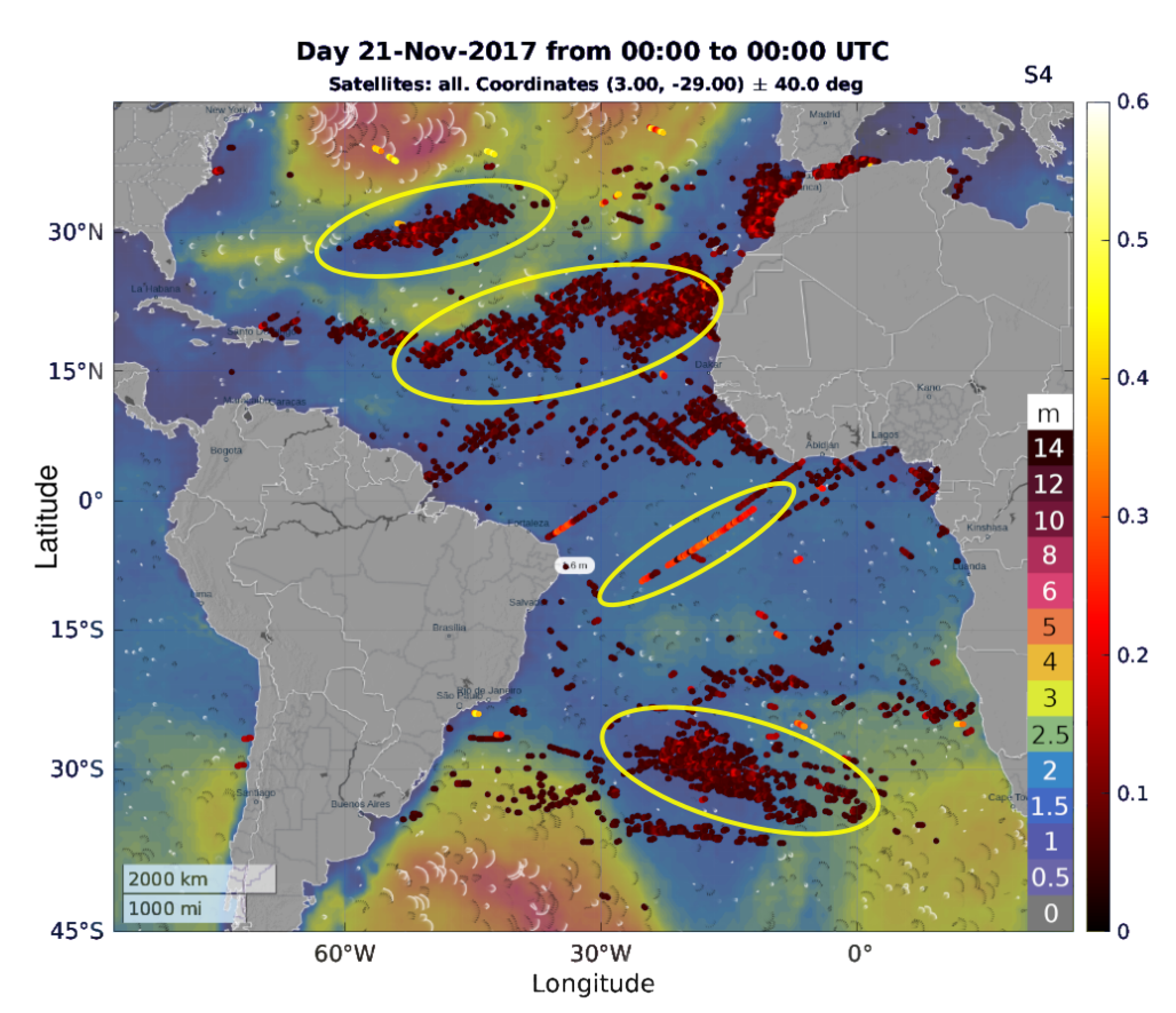
To check the wind and wave height for day and hour under study, ICON [16,17] model meteorological online data were used [18]. As an example, continuing with day 21 November 2017, in Figure 6, the colormap of wave-height along the Atlantic ocean is underlaid the values, only showing the ones that are larger than 0.05. It can be check that most of peaks only appear over regions with quite calm ocean.
3. Results
3.1. Bubbles and Depletions
Using the data available from the year 2017 until present, after applying the processing method described above, several interesting results found are shown. The research is mainly focused on the detection of Equatorial Plasma Bubbles (EPBs) or depletions. Given the characteristics of this experiment, these bubbles are expected to take the shape of transient peaks in curves as the reflected signal path crosses the bubble, while the GNSS receiver is moving along its orbit.
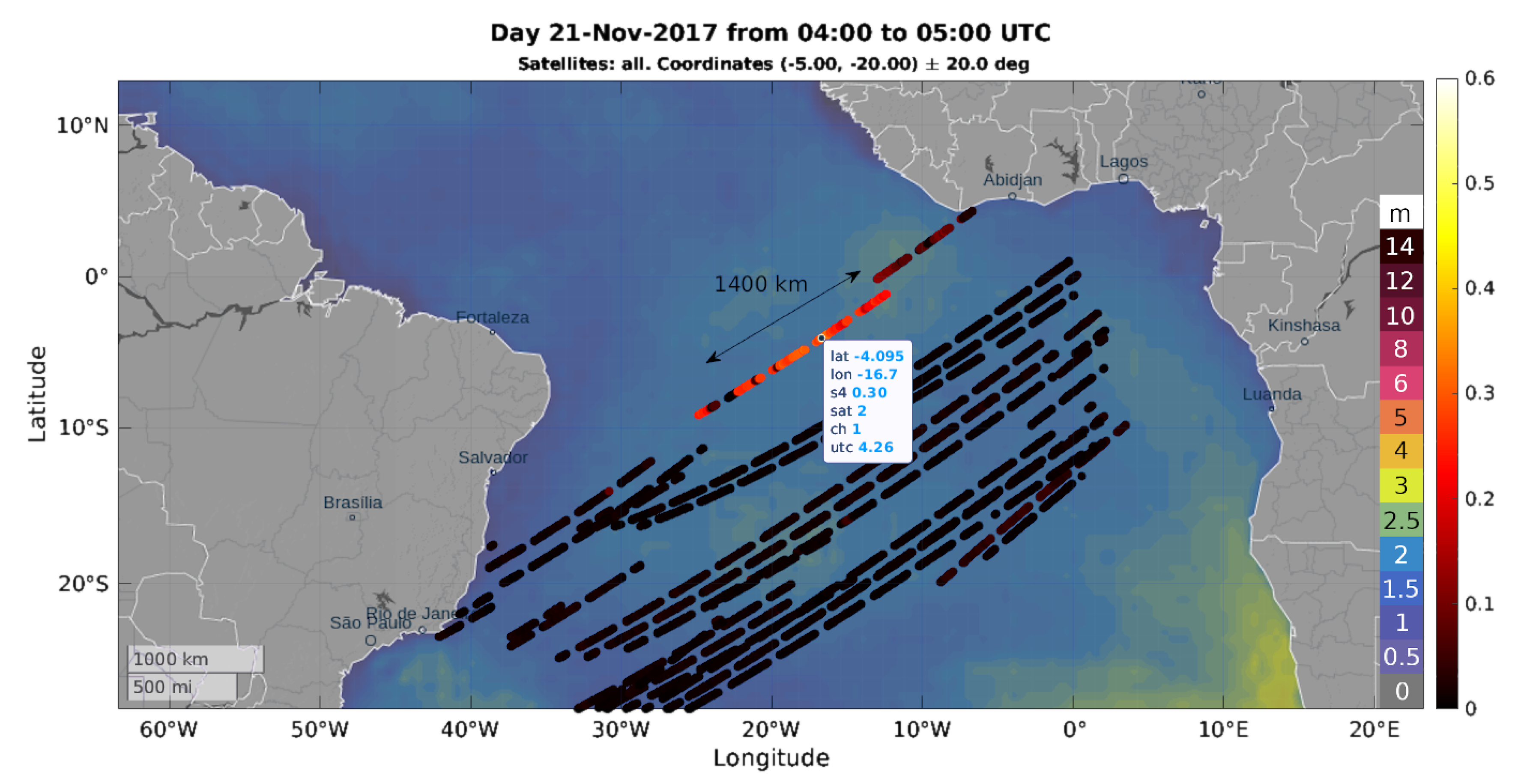
A first visual inspection of some days, like the one depicted before, shows that there are many peaks no matter which day is analyzed. Some of them are isolated, but others occur along with other peaks in slightly different times and other satellites or channels but in a relatively small region. One of these peaks in is located in mid the Atlantic during 21 November 2017, shown in Figure 7, and it may serve as an example to study its origin.
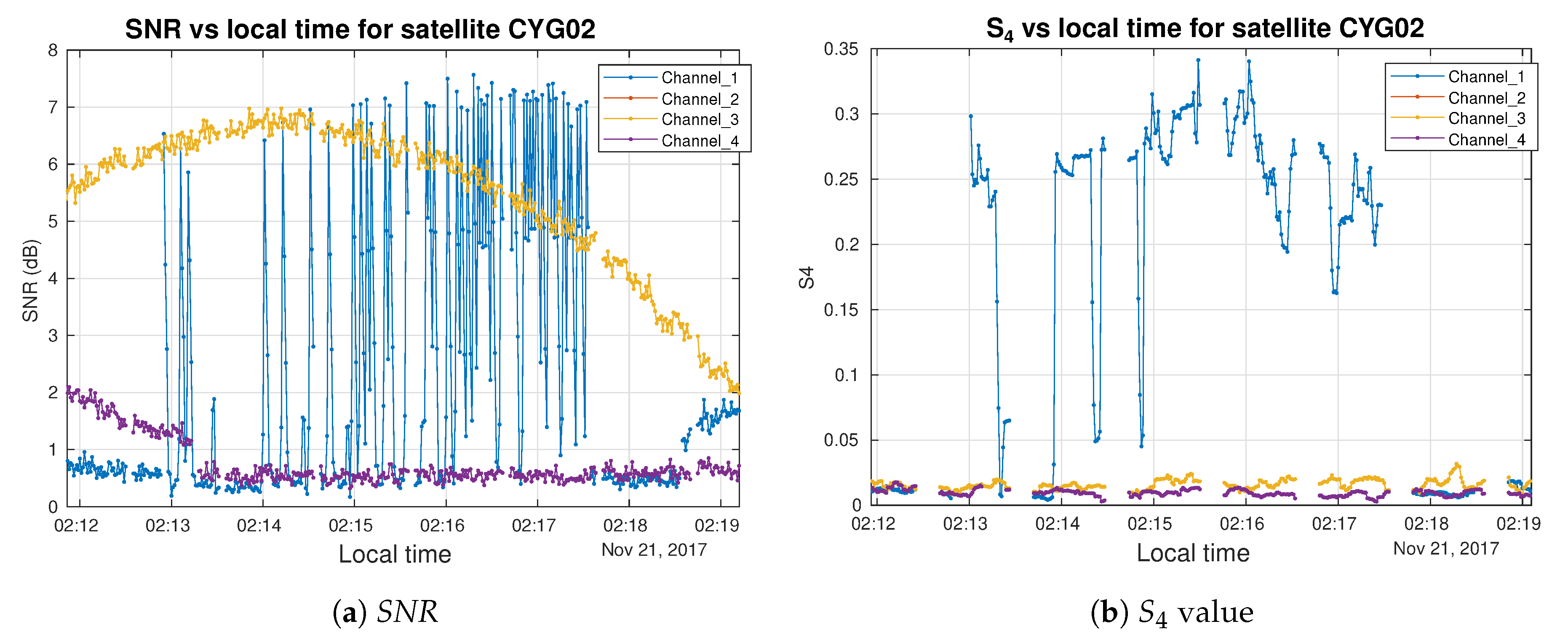
This isolated event in the Atlantic is the consequence of the rapid fluctuation of the SNR of the signal arriving to channel 1 of CYGNSS satellite 2, at around 4:26 UTC. The approximate length of the peak is 1400 km, and it lasts for about 5 minutes. As it can be seen in the SNR plot (Figure 8a), channel 1 oscillates rapidly from 1 dB to 7 dB, starting at 2:13 h to almost 2:18 h Local Time (LT), according to the longitude of the region. During this event, the ocean is calm, with wave heights of at most 2 m, as seen in Figure 6.
Also, these plots help to explain that, given the way the is computed, only the SNR fluctuations occurring in a timescale of 12 s can appear as high/moderate values. In channel 3 of the same satellite, a slow drift of the SNR is observed at the same time as channel 1 is fluctuating quickly (Figure 8a). Despite this, the value in channel 3 keeps being very small, less than 0.05 (Figure 8b). On the other hand, the singular parabolic shape that it exhibits is due to the change in the incident angle of the reflected signal as the receiver satellite moves in the orbit capturing the signal of the much slower and higher GPS transmitter. In this case, the angle of incidence is almost vertical (∼4), when the signal is maximum (∼7 dB), and increases up to around 25 at the end of the plot. In the case of channel 1, the angle of incidence varies less than 1 around 70 during all the fluctuation period.
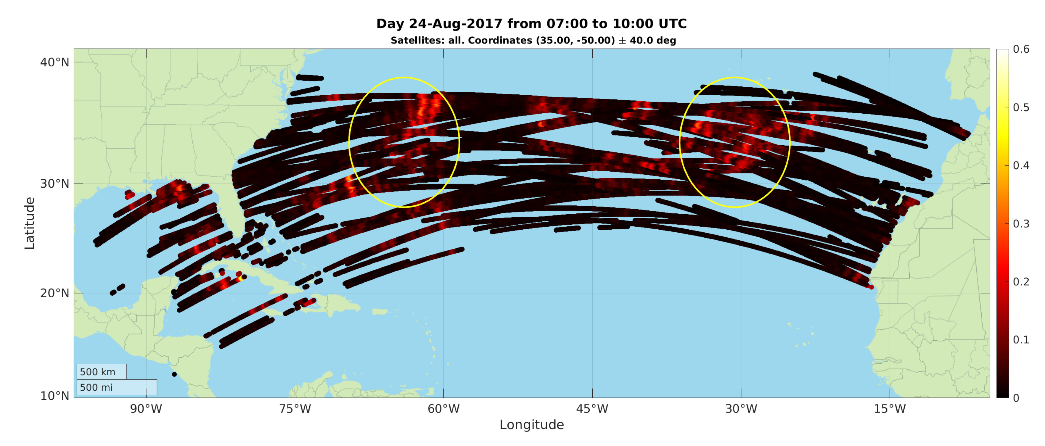
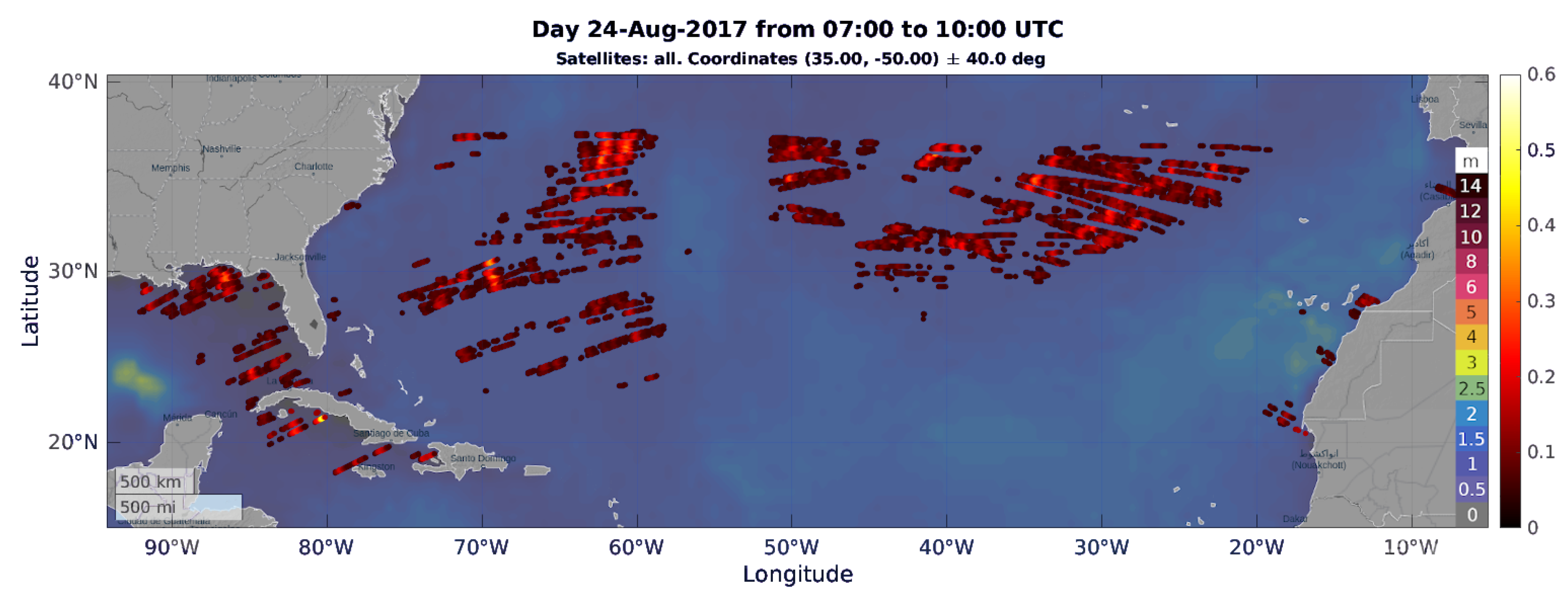
The previous example was an isolated peak in just one of the 4 channels of one satellite, but in other days analyzed, there are concentrations of these events in a small region, occurring during a finite time period. Figure 9 shows data from 24 August 2017. The points in red mark moderate scintillation measurements around 0.2–0.3, and they appear in some concentrated regions for different channels and satellites crossing above those regions. During this day, almost all the North Atlantic was very calm, with wave heights less than 2 m, as seen in Figure 10.
To have a better view of these events, two detail plots are shown.
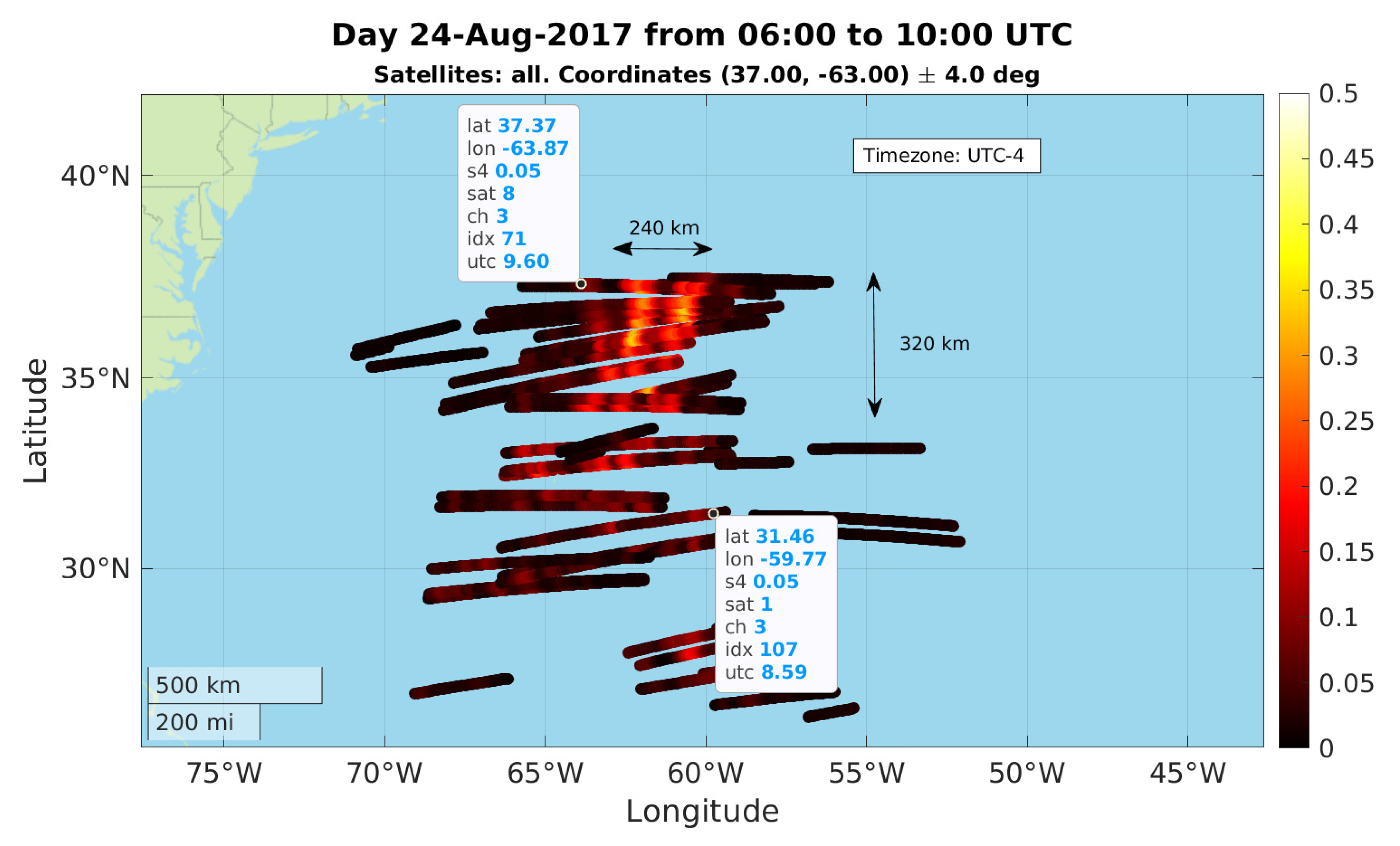
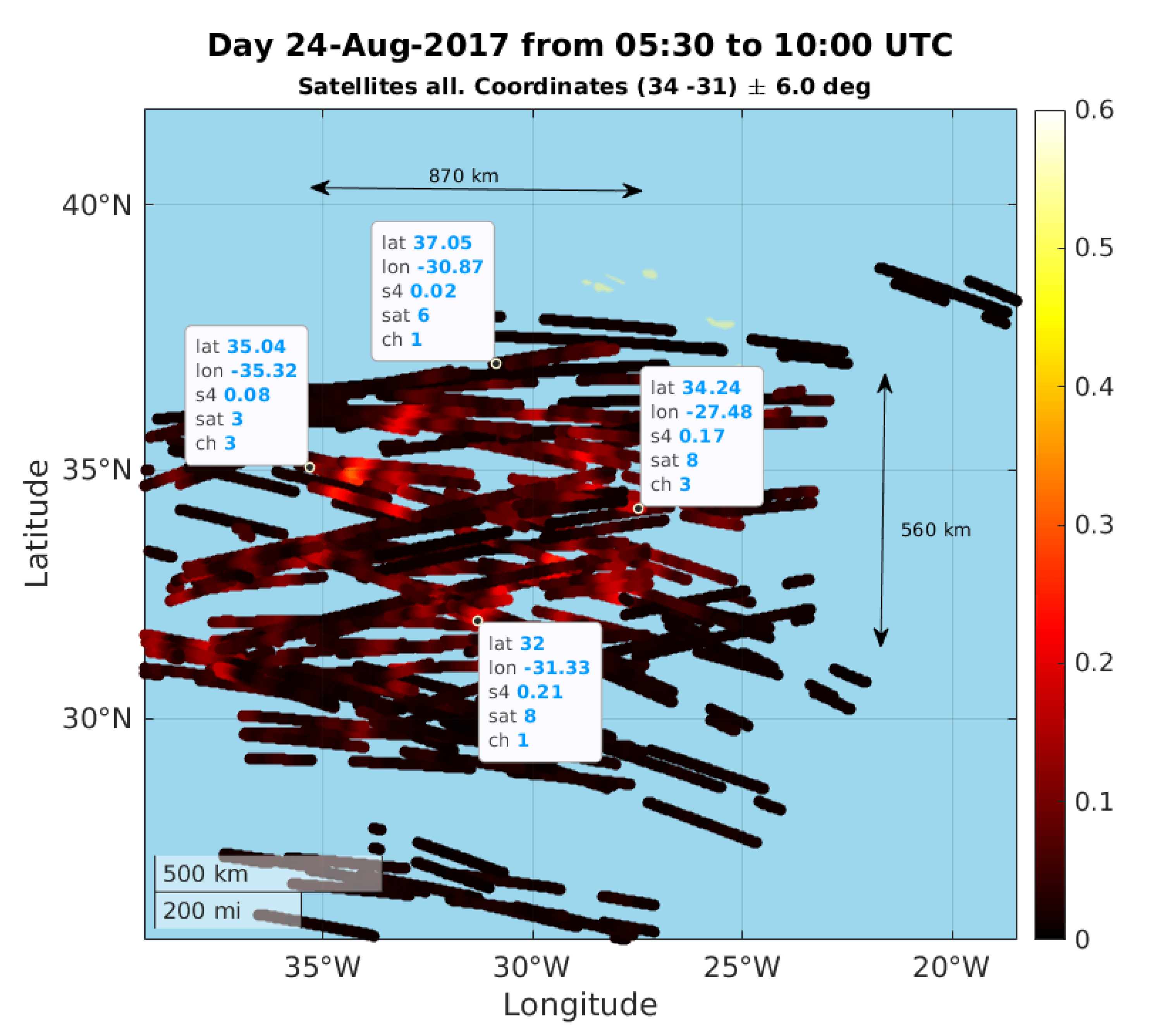
In the first one in the Western region, (Figure 11), located about 300 km North of Bermuda island, a large number of moderate points are closely spaced in a zone that extends approximately across different CYGNSS satellites and channels. All the measurements occur during the period between 6 h and 10 h UTC, even lasting during different passes of CYGNSS satellites over this zone.
In this region, the perturbation is particularly interesting as the peaks occur roughly at the same positions for several passes or channels, with similar values of in each of them. The event starts around 7:00 h UTC and ends around 10:00 h UTC, so given that the timezone is UTC-4, the local time is from 3 h to 6 h in the morning, coinciding with the hours immediately before the sunrise, that, in this place, on 24 August 2017, took place at 5:36 h LT.
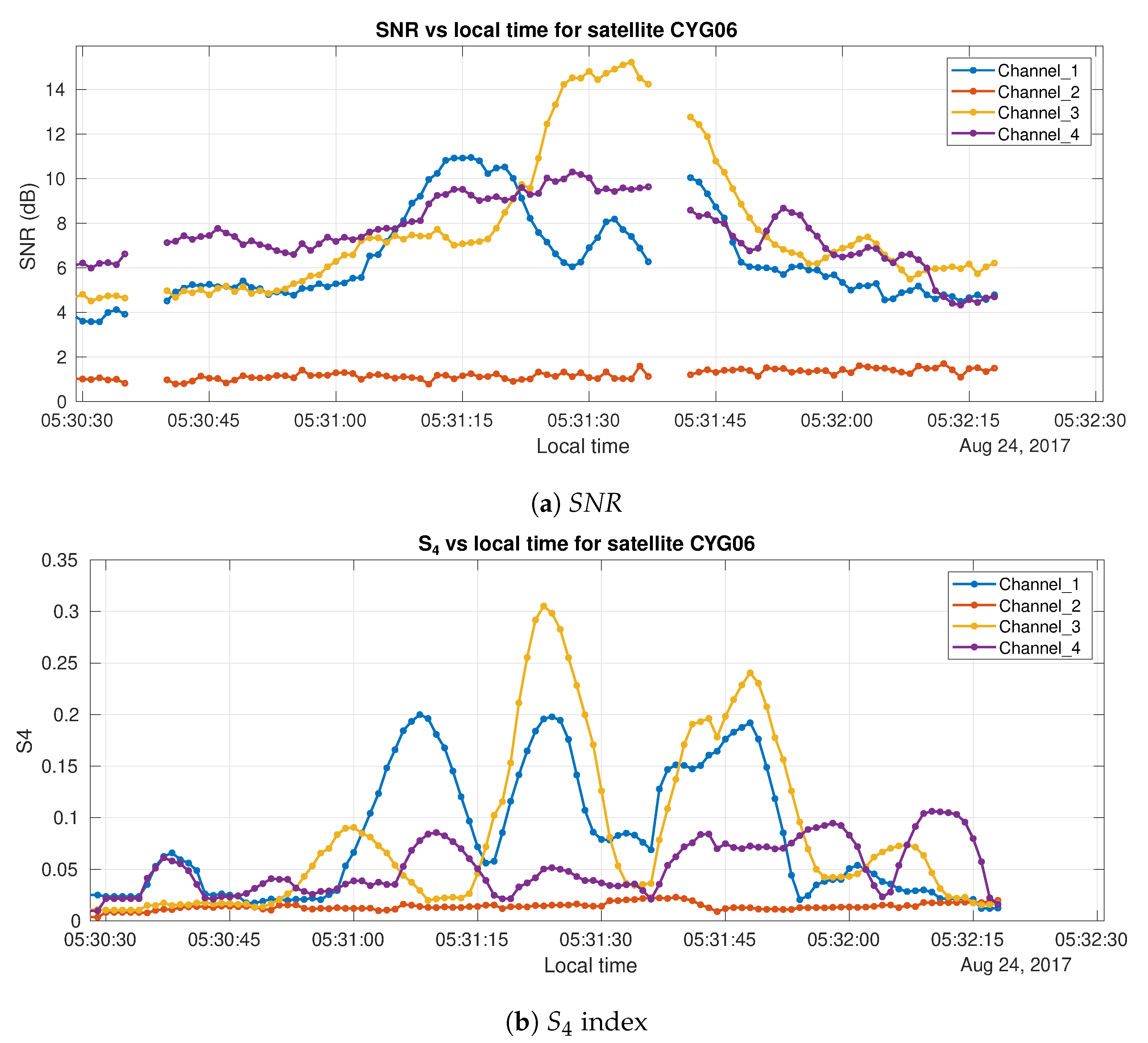
Focusing on this peak, the values of SNR and the derived are plotted in Figure 12a,b versus LT. The sudden increase of SNR values is clearly visible in two of the channels of the satellite CYG06. In other satellites (not shown in these graphs), there are also similar events, that constitute the peak in shown in Figure 11. It is important to note that the angle of the incident signal over the ocean is smoothly varying around 28 for channel 3, and from 14 to 10 in the case of channel 1, so the change in the reflection angle is not the cause of the rapid fluctuation of the signal.
In the map for the Eastern peak in North Atlantic (Figure 13), a region of about of moderate scintillation is depicted. As in the previous case, different passes of CYGNSS satellites in several channels show values of larger than 0.2. This region is around 200 km to 600 km southwest from the Azores islands, and the water surface was also in calm, as shown in previous Figure 10 for the whole day in almost all the North Atlantic ocean.
The information on these and other peaks is summarized in tables, recording for every event its date and time, duration, length, and magnitude of the value. In the data analysis these peaks are identified and characterized using the mentioned parameters. An event to be recorded must meet that the peak of must be larger than 0.2 during at least 5 s. Given that the integration window for computing is 12 s width, it means that a reported peak implies at least 17 seconds of fluctuations in the SNR of the received signal. Events shorter than this duration (or dimension) cannot be detected with the current coherent and incoherent integration times of the GNSS-R payload onboard. Table 2 shows the recorded peaks for 24 August 2017, from 7 h to 10 h (UTC), in all the North Atlantic region.
Table 2 shows the date and LT, the satellite and channel in which the peak was detected, the coordinates where the event started, its duration and length, the inclination of the incident signal on the sea (measured from the vertical), and the maximum value of achieved during the peak. The length of the event is computed measuring the distance between the first and the last geolocated points belonging to the peak.
Note that the highlighted row in Table 2 corresponds to the peak measured by satellite 6 in channel 3 on (37.27N, 62.21W) at 5:31 LT, which is the one plotted in yellow in Figure 12a,b. As it can be seen, the peak lasts for 7 seconds over the threshold of 0.2, archiving a maximum height of 0.31.
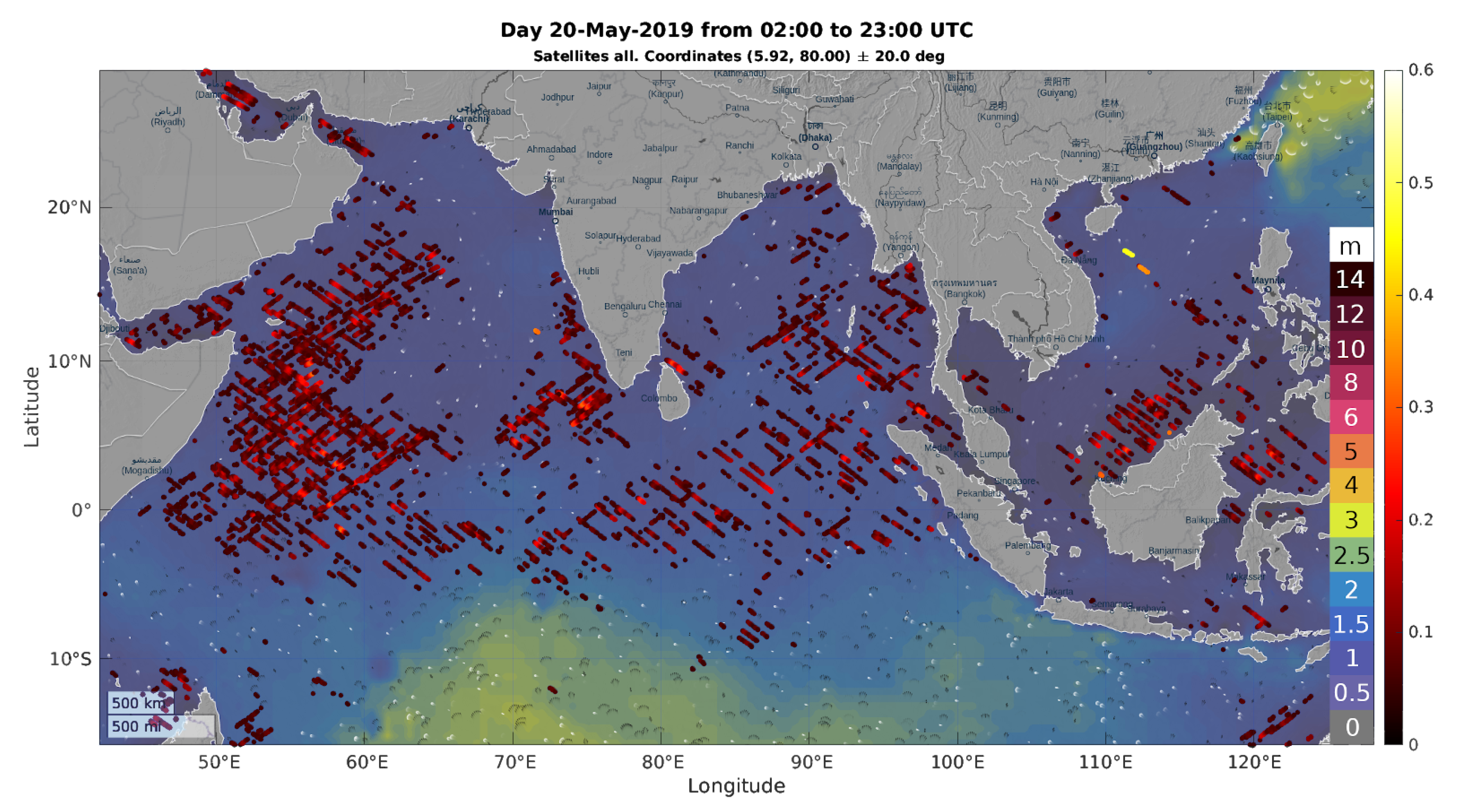
Another day of interesting results, this case in the Indian Ocean during 20 May 2019, is shown in Figure 14. As seen in the plot, the Indian Ocean was calm during that day in regions from the Equator to the North. The plot only shows the values greater than 0.05, and they are distributed in regions relatively delimited between the Equator and latitude 15N.
Table 3 shows peaks above 0.2 lasting for at least 5 s during that day, indicating its properties.
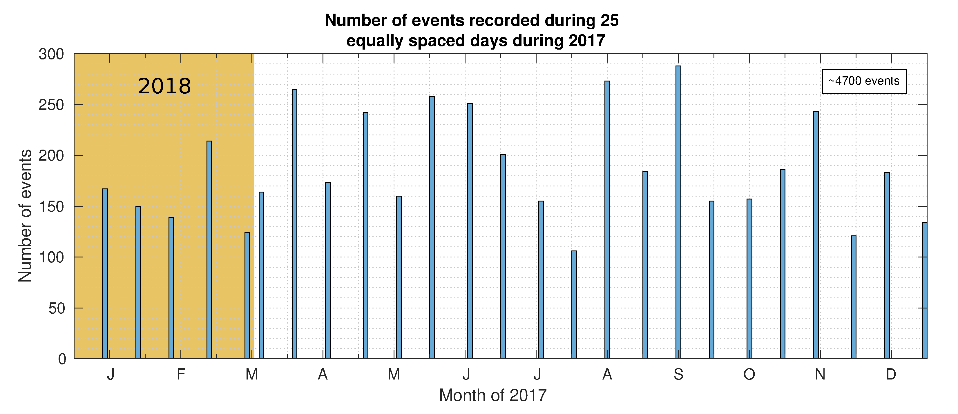
Better statistics can be extracted by obtaining these tables for a large number of days. In the following lines, the study of 25 days equally distributed every 15 days from March 2017 to March 2018 is presented. The methodology used is to parse the whole day in all the oceanic regions from 40N to 40S recording the events with above 0.2 lasting more than 5 s. The number of peaks recorded per day in the year is shown in Figure 15.
3.2. S4 Statistics
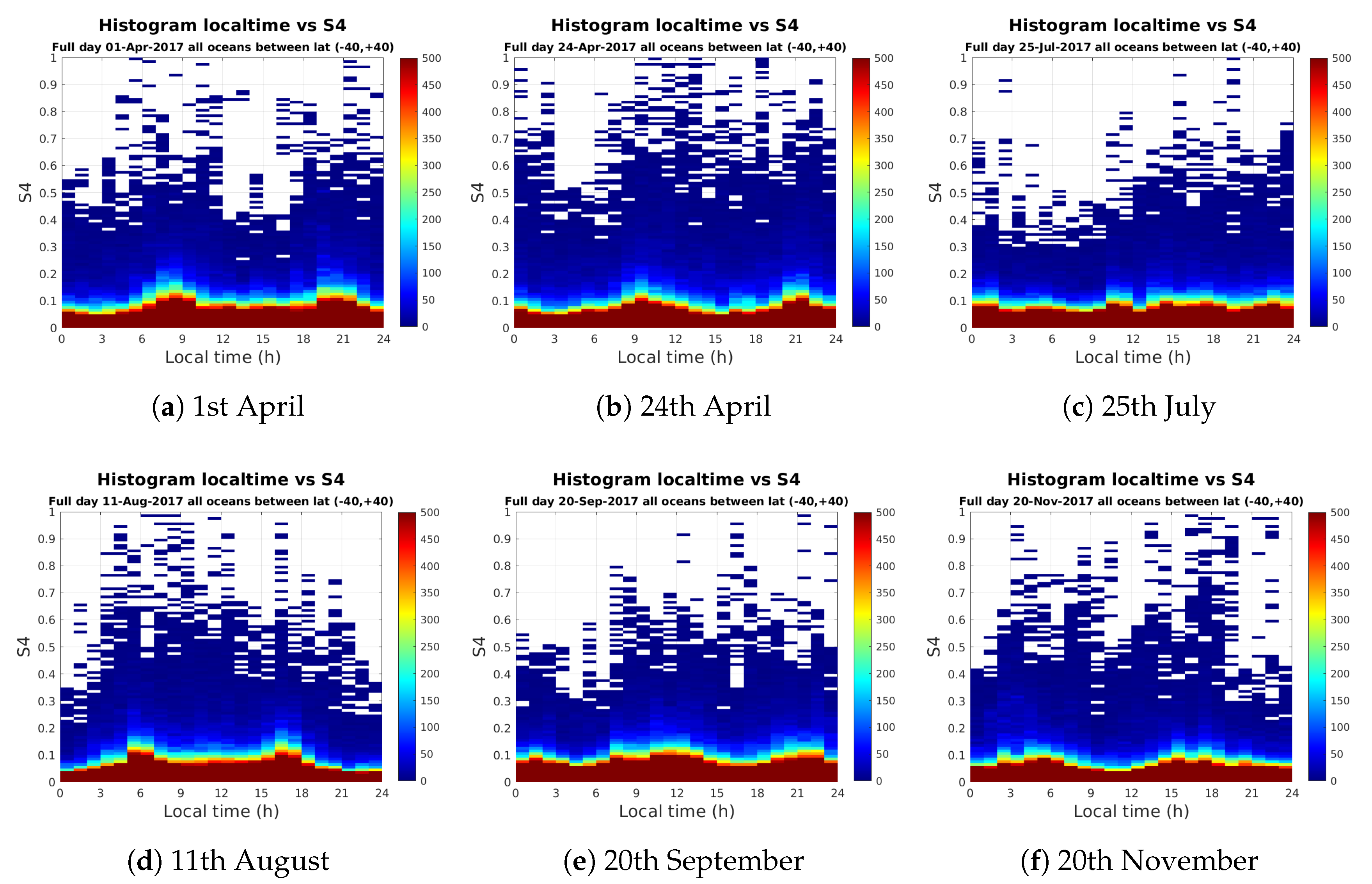
Another analysis conducted, is the study of the probability to find points with certain at a particular hour in LT, averaging the data over long periods of time. This way, it can be studied if there is any correlation between the obtained with this technique and the LT, as previous models and experimental evidence shows. The set of histograms in Figure 18 shows all the data points from 0 h to 24 h (UTC) during selected days in the year 2017.
The horizontal axis of the histograms represents the local time in hourly bins, and the vertical scale is the value in bins of 0.1. The color represents the number of counts per each of the two-dimensional bins. The color scale is adjusted up to 500 counts to increase the contrast for values larger than 0.1. This means that all the bins in red on the bottom side of the histogram are saturated.
The data plotted in the histograms correspond to all the specular reflections over open oceans and seas (further away than 50 km from any coastline), within the latitudes of CYGNSS coverage (40N, 40S). In total, every day there are approximately samples. The registered values include all reflections on the cited areas without any other filter (i.e., no sea surface roughness filter).
In these histograms, a small dependency with LT can be observed, that is more visible in April and August, with a slightly higher probability of higher during sunrise and sunset, around 6 h and 17 h during 21st August, and 9 h and 21 h during both days in April. Also, a similar correlation can be observed on 20th November.
4. Discussion
The results presented in this study are consistent with previous observations and studies. As a general starting point, several peaks in are found in many days during the years of operations of the CYGNSS mission.
One of the main concerns during the study was the need to filter the GNSS reflections only for coherent reflections, as ionospheric scintillation may only be “visible” when a coherent wave crosses the ionosphere. In practice, this means that the signal has to be reflected over calm water. That is the reason why in every particular case, the wave height and winds speed maps were checked before a more in-depth analysis was performed to the data. For example, two of the days shown, 24 August 2017 (Figure 10) and 21 November 2017 (Figure 6), exhibit calm sea on the regions of interest where some scintillation was found.
4.1. Bubbles Study
Obtained results match with previous studies and, in some cases, they can be clearly interpreted as the EPBs described, for example, in Reference [19]. In this work, a method for detecting and measure equatorial plasma depletions is explained. These depletions in the electron content of the ionosphere highly affect the radio wave signals crossing them, and they can rapidly appear, travel some distance, and then vanish. The way to study them in Reference [19] is by the use of data provided by ground-based GNSS receivers belonging to the International GNSS Service (IGS), available online since, at least, 2002, including different solar cycles.
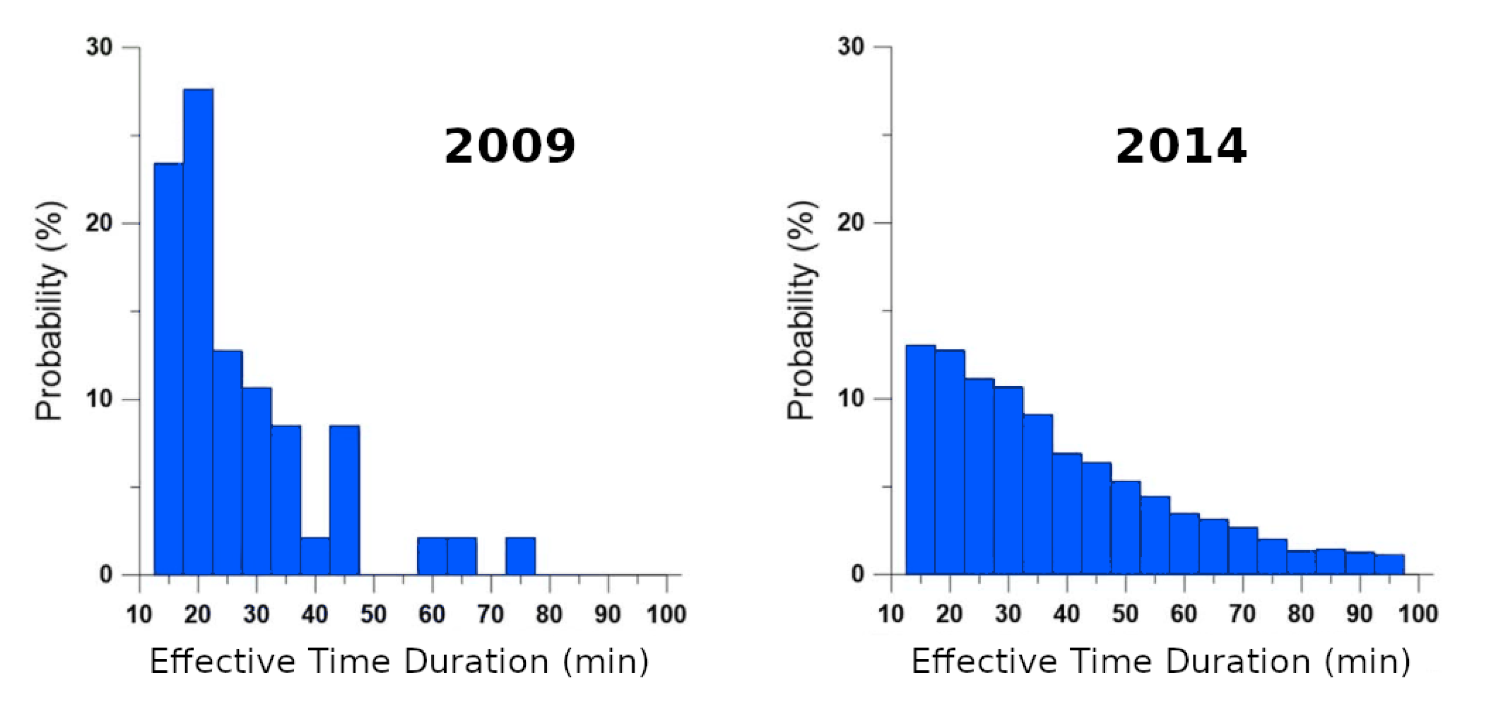
GNSS satellites orbit at 20,000 km altitude (GPS), with periods of 12 h, which means that from a ground station they are in view during long times, making it possible to study the region of the ionosphere that crosses the vector from the satellite to the receiver. As this vector moves slowly compared to the estimated drift velocity of the plasma bubbles, they can cross the signal path during the tracking of a single GNSS satellite. This method is applied systematically to measure the duration and depth of these bubbles. The results show that these bubbles could have very different duration, lasting from 10 to almost 100 min during a solar maximum, or shorter periods during a solar minimum, as shown in Figure 19.
In order to make a comparison between both studies, the equivalent length of the bubbles has been computed. Regarding the measurement from ground stations and neglecting the movement of the GNSS satellites during the transition of the bubble, the length of the bubbles can be estimated using the mean drift velocity of the ionospheric plasma, ∼100 m/s. That transformation linearly translates the horizontal scale of Figure 19, from 10–100 min to 60–600 km, respectively.
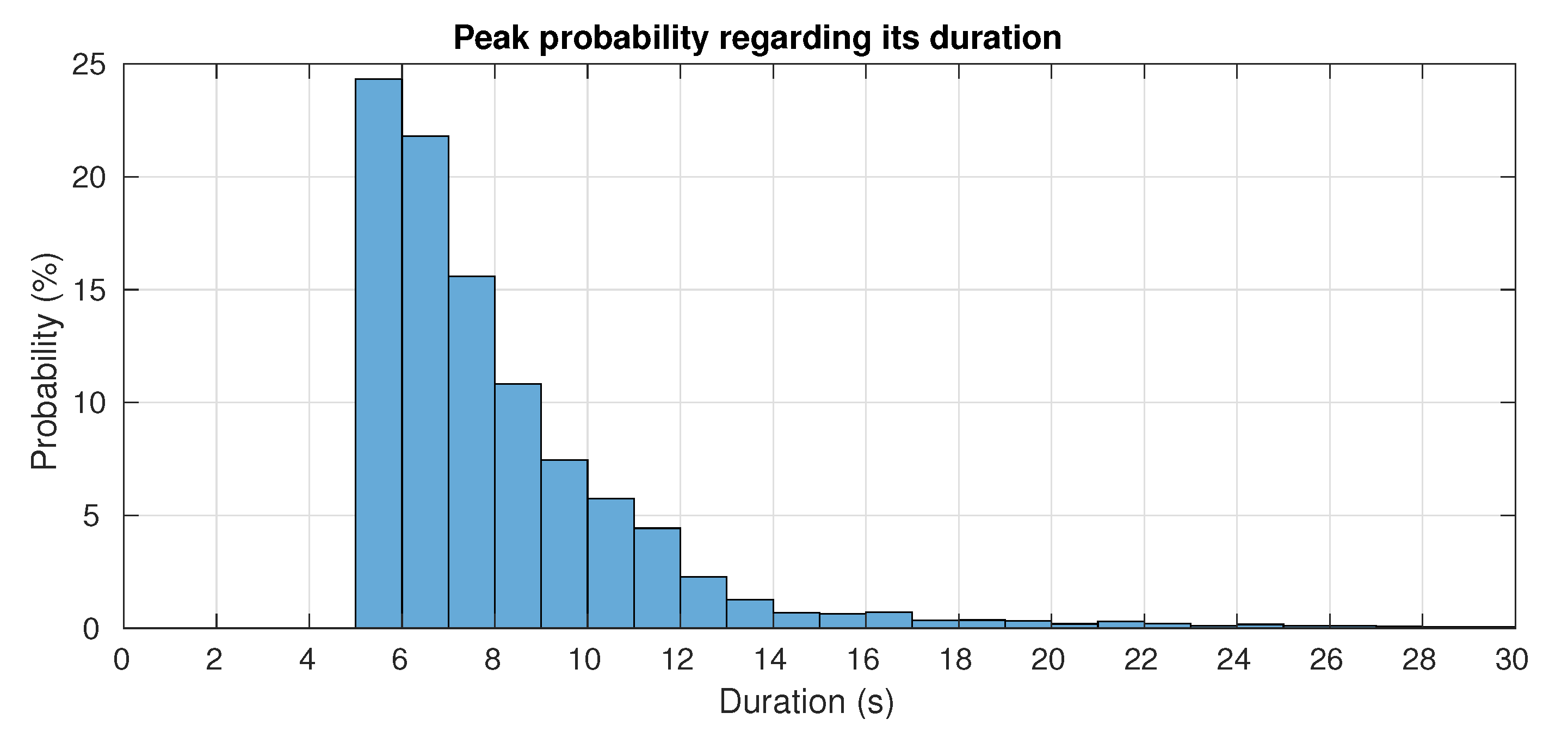
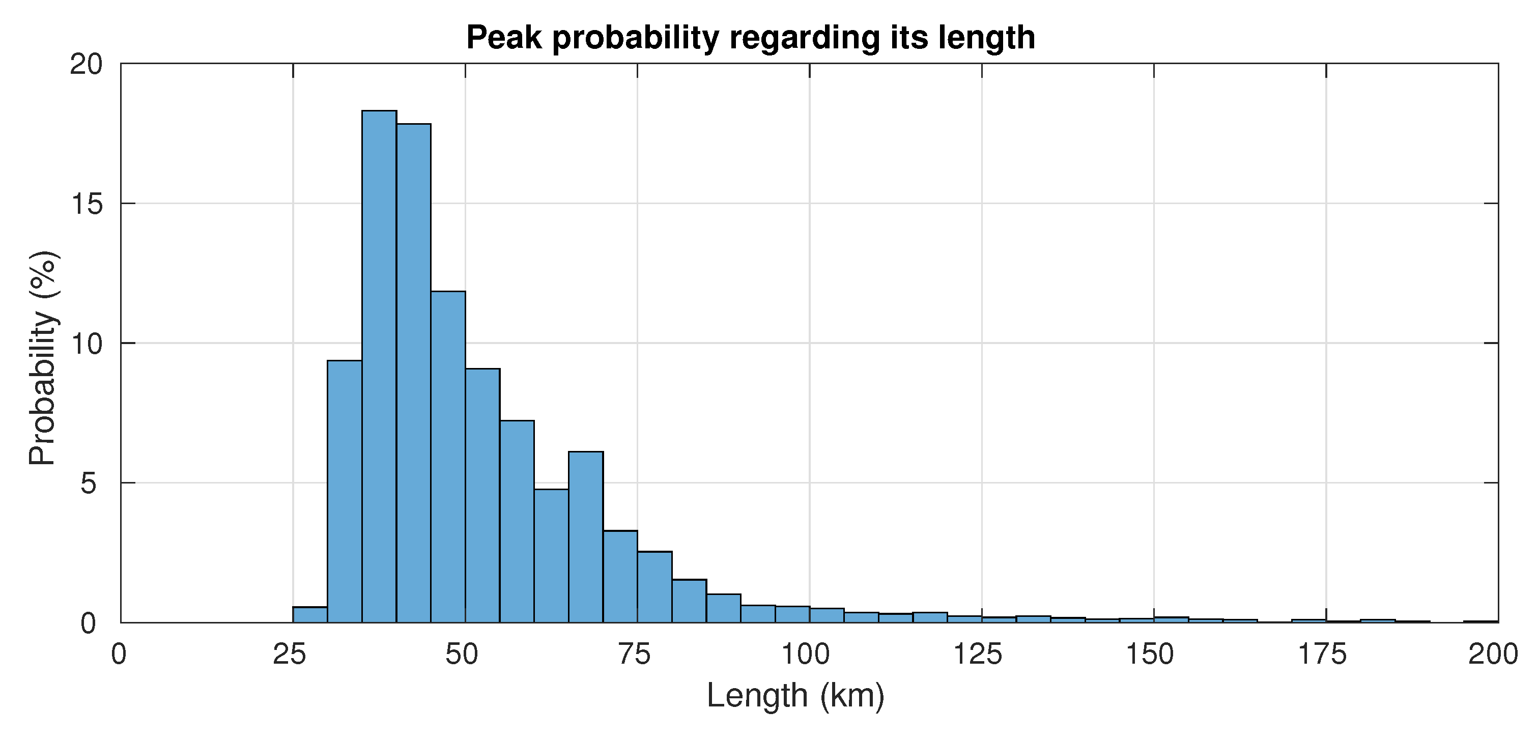
From the recorded CYGNSS data, using equally spaced days every 15 days from March 2017 to March 2018 –25 days in total–, all the peaks lasting more than 5 s with an value above 0.2 have been computed to display the histogram shown in Figure 20. The extension of the bubble, in this case, is computed from the coordinates of the first and last specular reflection considered part of the peak and it is shown in Figure 21. The total number of peaks analyzed in these histograms is around 4700 and they are distributed along the 25 days in 2017 using the data shown in the previous section represented in Figure 15.
Comparing CYGNSS data with the one studied in Reference [19], many similarities can be extracted. The shape of the distribution fits very well in terms of bubble extension, ranging from around 40 km to 200 km. In both plots, an exponential-like shape can be observed.
4.2. Correlation to Local Time
Another aspect to highlight is the correlation between local time and the occurrence of high events, as shown in the set of histograms in Figure 18. Some of them show a higher probability of finding high values during hours around the sunrise and sunset. In particular, plots on 1 and 24 April, which are also very similar to each other, reveal peaks around 9 h in the morning and 8–9 h in the evening. It is also important to remark that the sunrise and sunset do not occur at the same time in all the regions covered in this graphs, which are all the oceans and seas with latitudes from 40N to 40S. Considering April is close to the equinox, the span between local sunrise and sunset is not very large from 40N to 40S: around 30 min. It would be exactly zero on the equinoxes. This difference is much higher for 25 July, around 2 h 20 min.
In this way, being the sunrise and sunset the most active periods in terms of ionospheric activity, in the equinoxes the peak in these histograms should be even higher than in the solstices because, during the equinoxes, sunrise and sunset happen at the same time for all latitudes. This can be observed in the July histogram (Figure 18c), but it is not evident in the November’s one (Figure 18f). However, it is important to consider that the measurements used for these histograms have no sea roughness filter, and they use all the data over oceans within CYGNSS available latitudes.
4.3. Comparison with Plasma Density Data from Swarm
ESA Swarm mission is a constellation of 3 satellites launched in 2013 that globally provides data on the geomagnetic field and plasma density. Satellites named as Swarm A and C fly together in a polar orbit of around 460 km altitude and 87.4 inclination, so they can sense the plasma density on the ionosphere. Swarm B is orbiting at 530 km, within another polar orbit plane, so it can sense a bit higher layer of the ionosphere. Swarm instruments can measure geomagnetic field intensity and direction, and also, local electron plasma density.
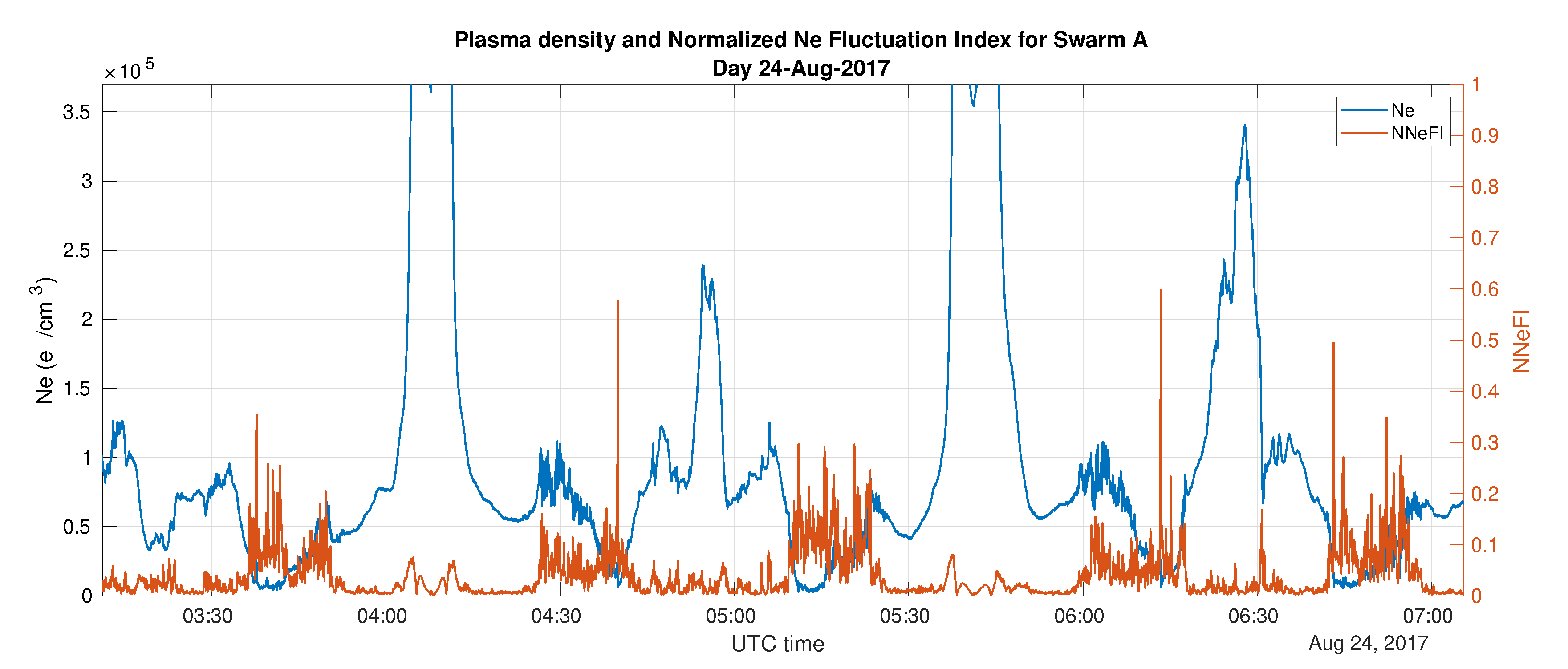
In order to compare with previous results from CYGNSS, Swarm measurements during 24 August 2017 have been analyzed. In Figure 22, the plasma density during some hours of this day is plot along with an index that the authors have defined to indicate the intensity of its fluctuations, the Normalized Ne Fluctuation Index (NNeFI). This index is obtained from the plasma density given by Swarm (Ne), once per second. Ne measures the number of electrons per cubic centimeter with values that are in the order of , the typical electron density in the ionosphere at this height. Using Ne, the NNeFI is computed as:
where Ne is the electron density measured by Swarm and the average is computed using a 12-samples moving window.
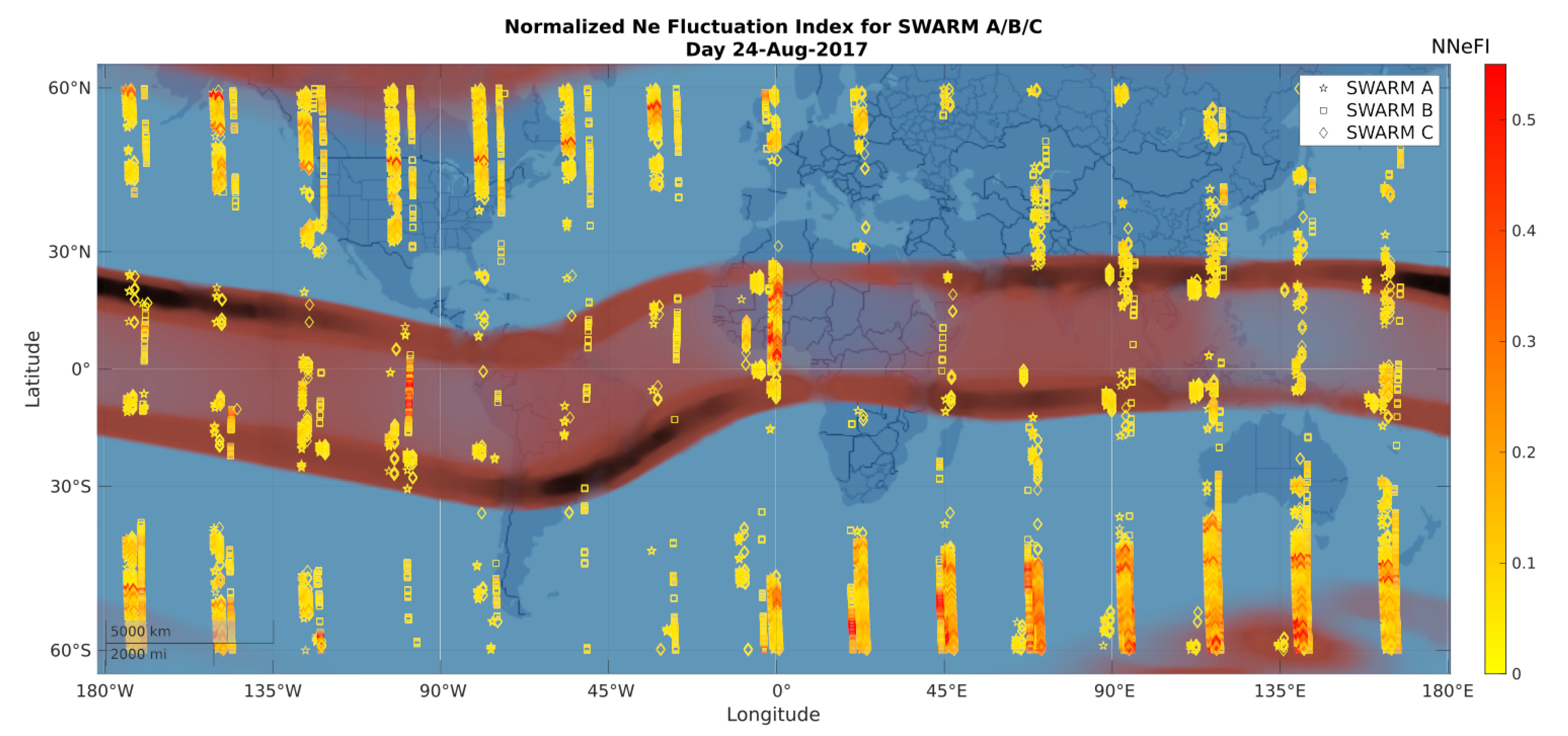
This index is plotted in a map in Figure 23, for the whole day and the three Swarm satellites, and it is underlaid the mean occurrence of scintillation events, using the WBMOD model predictions of the percentile index. Note that only values of NNeFI above 0.05 are shown. It can be observed a correlation between the appearance of plasma density fluctuations and the predicted map.
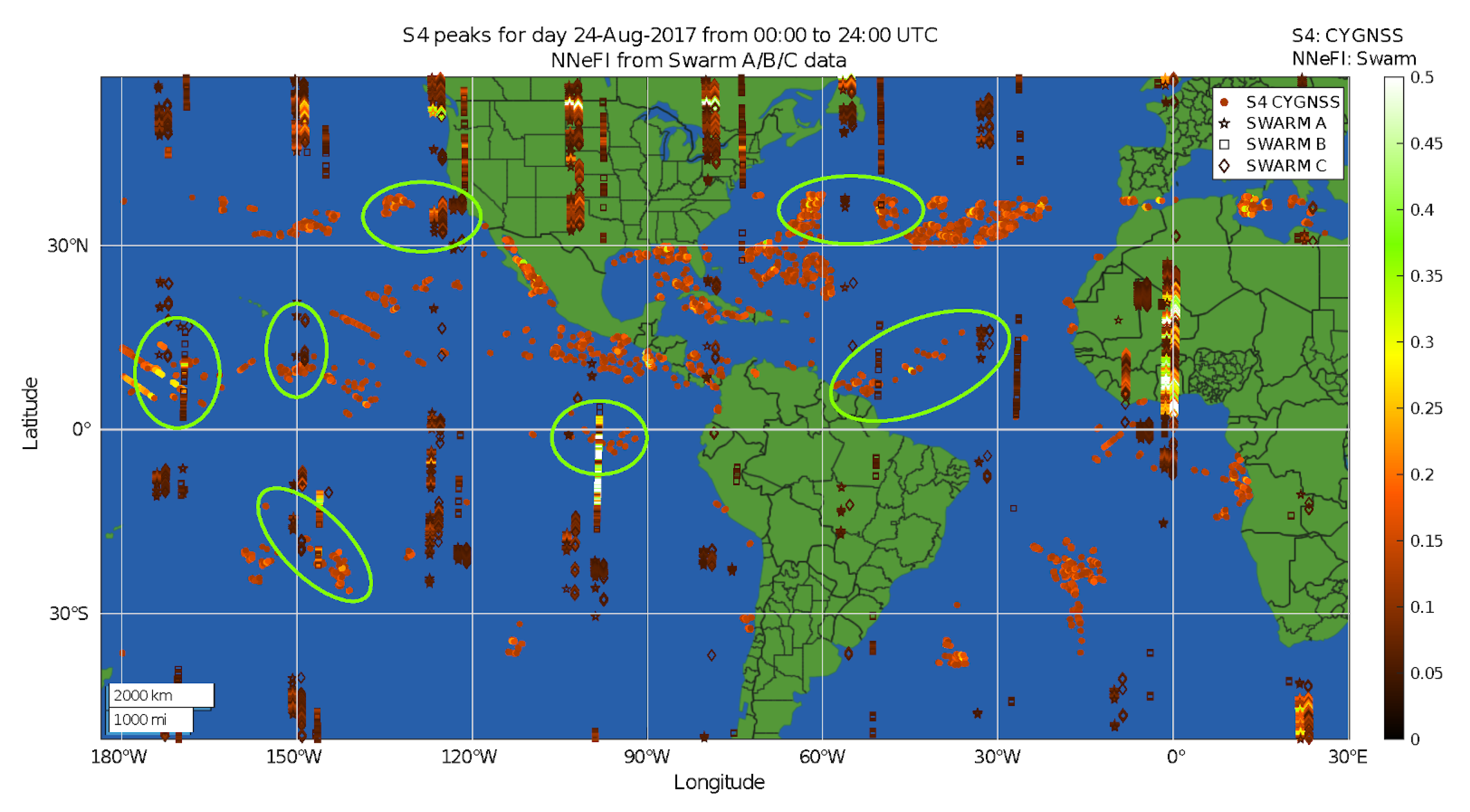
In Figure 24 it is plotted the same data from Swarm NNeFI along with the peaks of reported by CYGNSS during the same day that was studied in previous sections of this work. values plotted are filtered to be higher than 0.12. Swarm computed NNeFI exhibits high occurrence in high latitudes, above 60, both Northern and Southern, but they are out of the region covered by CYGNSS and they will be not mentioned here.
Around meridian 0 there is a large region of fluctuations observed by Swarm A and C, over Sahara and Ghana, which, in the part that enters to the Atlantic ocean, there is also some peaks detectable by CYGNSS. Another example is found in the line of peaks that goes from The Guianas to Cabo Verde that seems to be completed with some peaks in the NNeFI index from Swarm B. There is also some cases along the Pacific Ocean that are marked with circles, where there is a cluster of peaks at the same time as NNeFI peaks. There are also other regions in which there is mostly peaks but few or none Swarm indicators, for example in the South of Mexico, in the region between Bermudas and Cuba or in the Middle South Atlantic
It is important to note that the availability of data is much larger in the CYGNSS constellation than the Swarm one. For one day, CYGNSS has 8 satellites with 4 channels each in a orbit with less inclination; Swarm is only three satellites in polar orbit. This fact could difficult the correlation between both databases, but here, there are some evidences that motivates further study.
5. Conclusions
This work has presented the first experimental evidence that GNSS-R can be used as a global ionospheric scintillation monitor, and in particular, of bubble and depletions. Future work on the search of ionospheric activity at all latitudes and during different solar activity periods could help in the improvement of existing ionospheric models, providing them with more complementary data than ground stations are currently providing and with a denser spatial coverage than Swarm mission.
The study shows the result of scintillation events during the years 2017 and 2019, including tables with peaks that correspond to EPBs that are consistent with previous studies in terms of duration, LT, and also latitudes. The duration of the events shown here is in the order of seconds (from 5 s to 30 s), which means bubbles of around 25 km to 150 km length. The depth of these bubbles in terms of maximum is in the order of 0.2 to 0.5.
This way to study the ionospheric scintillation could be very beneficial because it can cover large areas all over the Earth, including remote regions in the middle of oceans, where no ground stations could be placed. However, there is also has some limitations and they should be carefully identified and refined. One of them is that only calm ocean surfaces ensure coherent specular reflections. If the water surface has ripples, the signal would reflect from a larger glistening zone, arriving at the receiver with different phases, hiding the possible fluctuations in amplitude and phase. In further studies continuing the analysis of CYGNSS and other GNSS-R missions, an automated data filtering algorithm must be implemented to eliminate data affected by sea roughness.
On the other hand, it is important to take into account that the results presented in the study come from years 2017 to 2019, and solar activity cycle should reach its minimum in 2020. That implies that less activity is expected, and consequently, fewer scintillation events. It would be very interesting to study GNSS-R data from future missions when approaching the solar maximum.
A correlation study between these results and others obtained from different sources, for example, the Swarm geomagnetic and plasma density products is being performed to find possible confirmations of this new proposed technique and also to check what new possibilities could GNSS-R technique bring to the ionospheric monitoring field.
The results presented in this study are a small sample of the total amount of information that can be obtained using this technique. CYGNSS generates around 10.4 GB per day, and further exhaustive analyses of it could bring new information or improve current models of the ionosphere, which is especially interesting regarding oceanic regions.
Author Contributions
Conceptualization, C.M. and A.C.; methodology, C.M. and A.C.; software, C.M.; validation, C.M. and A.C.; formal analysis, C.M. and A.C.; investigation, C.M.; resources, A.C.; data curation, C.M.; writing–original draft preparation, C.M.; writing–review and editing, C.M. and A.C.; visualization, C.M.; supervision, A.C.; project administration, A.C.; funding acquisition, A.C. All authors have read and agreed to the published version of the manuscript.
Funding
This work has been partially funded by the Spanish MCIU and EU ERDF project (RTI2018-099008-B-C21/AEI/10.13039/501100011033) “Pioneering Opportunistic Techniques”, grant to “CommSensLab-UPC” Excellence Research Unit Maria de Maeztu (MINECO grant MDM-2016-600), and ESA project AO 1-8862/17/NL/AF/eg “RADIO CLIMATOLOGY MODELS OF THE IONOSPHERE: STATUS AND WAY FORWARD”.
Acknowledgments
Thanks to the CommsSensLab administrative and research personnel and to the NanoSatLab members for all the support. Special thanks to Badr-Eddine Boudriki for his help in Swarm data retrieval and pre-processing, and to Hyuk Park for his wise advises and comments on this study.
Conflicts of Interest
The authors declare no conflict of interest.
Abbreviations
The following abbreviations are used in this manuscript:
| EPB | Equatorial Plasma Bubble |
| ESA | European Space Agency |
| GISM | Globa Ionospheric Scintillation Model |
| GNSS | GeoNavigation Satellite System |
| GNSS-R | GNSS Reflectometry |
| GPS | Global Positioning System |
| ITU-R | International Telecommunications Union, Radiocommunication Sector |
| LEO | Low Earth Orbit |
| LT | Local Time |
| NNeFI | Normalized Ne Fluctuation Index |
| PO.DAAC | Physical Oceanography Distributed Active Archive Center |
| SNR | Signal-to-Noise Ratio |
| UTC | Coordinated Universal Time |
References
- Béniguel, Y. Global Ionospheric Propagation Model (GIM): A propagation model for scintillations of transmitted signals. Radio Sci. 2002, 37, 4-1–4-13. [Google Scholar] [CrossRef] [Green Version]
- Knepp, D.L. Multiple phase-screen calculation of the temporal behavior of stochastic waves. Proc. IEEE 1983, 71, 722–737. [Google Scholar] [CrossRef]
- ITU. Ionospheric Propagation Data and Prediction Methods Required for the Design of Satellite Services and Systems. Recommendation ITU-R531-10; International Telecommunication Union: Geneva, Switzerland, 2017; Available online: https://www.itu.int/rec/R-REC-P.531-10-200910-S/en (accessed on 18 October 2020).
- Fremouw, E.J.; Secan, J.A. Modeling and scientific application of scintillation results. Radio Sci. 1984, 19, 687–694. [Google Scholar] [CrossRef] [Green Version]
- Wernik, A.W.; Alfonsi, L.; Materassi, M. Scintillation modeling using in situ data. Radio Sci. 2007, 42, 1–21. [Google Scholar] [CrossRef] [Green Version]
- Camps, A.; Barbosa, J.; Juan, M.; Blanch, E.; Altadill, D.; González, G.; Vazquez, G.; Riba, J.; Orús, R. Improved modelling of ionospheric disturbances for remote sensing and navigation. In Proceedings of the 2017 IEEE International Geoscience and Remote Sensing Symposium (IGARSS), Fort Worth, TX, USA, 23–28 July 2017; pp. 2682–2685. [Google Scholar]
- Tulasi Ram, S.; Ajith, K.K.; Yokoyama, T.; Yamamoto, M.; Niranjan, K. Vertical rise velocity of equatorial plasma bubbles estimated from Equatorial Atmosphere Radar (EAR) observations and HIRB model simulations. J. Geophys. Res. Space Phys. 2017, 122, 6584–6594. [Google Scholar] [CrossRef]
- Camps, A.; Park, H.; Foti, G.; Gommenginger, C. Ionospheric Effects in GNSS-Reflectometry From Space. IEEE J. Sel. Top. Appl. Earth Obs. Remote Sens. 2016, 9, 5851–5861. [Google Scholar] [CrossRef]
- Katzberg, S.J.; Garrison, J.L. Utilizing GPS to Determine Ionospheric Delay over the Ocean; NASA Technical Memorandum 4750; NASA: Hampton, VA, USA, 1996.
- Garrison, J.L.; Katzberg, S.J. Detection of ocean reflected GPS signals: Theory and experiment. In Proceedings of the IEEE SOUTHEASTCON ’97, ‘Engineering the New Century’, Blacksburg, VA, USA, 12–14 April 1997; pp. 290–294. [Google Scholar]
- Ye, Z.; Satorius, H. Channel modeling and simulation for mobile user objective system (MUOS)—Part 1: Flat scintillation and fading. In Proceedings of the IEEE International Conference on Communications, 2003, ICC’03, Anchorage, AK, USA, 11–15 May 2003. [Google Scholar] [CrossRef]
- Ruf, C.; Gleason, S.; Jelenak, Z.; Katzberg, S.; Ridley, A.; Rose, R.; Scherrer, J.; Zavorotny, V. The NASA EV-2 Cyclone Global Navigation Satellite System (CYGNSS) mission. In Proceedings of the 2013 IEEE Aerospace Conference, Big Sky, MT, USA, 2–9 March 2013; pp. 1–7. [Google Scholar]
- Ruf, C.; Gleason, S.; Ridley, A.; Rose, R.; Scherrer, J. The Nasa CYGNSS Mission: Overview and Status Update. In Proceedings of the 2017 IEEE International Geoscience and Remote Sensing Symposium (IGARSS), Fort Worth, TX, USA, 23–28 July 2017; pp. 2641–2643. [Google Scholar]
- CYGNSS. CYGNSS Level 1 Science Data Record Version 2.1. 2018. Available online: https://podaac.jpl.nasa.gov/dataset/CYGNSS_L1_V2.1 (accessed on 8 September 2020).
- Zavorotny, V.U.; Gleason, S.; Cardellach, E.; Camps, A. Tutorial on Remote Sensing Using GNSS Bistatic Radar of Opportunity. IEEE Geosci. Remote Sens. Mag. 2014, 2, 8–45. [Google Scholar] [CrossRef] [Green Version]
- Korn, P. Formulation of an unstructured grid model for global ocean dynamics. J. Comput. Phys. 2017, 339, 525–552. [Google Scholar] [CrossRef]
- Giorgetta, M.A.; Brokopf, R.; Crueger, T.; Esch, M.; Fiedler, S.; Helmert, J.; Hohenegger, C.; Kornblueh, L.; Köhler, M.; Manzini, E.; et al. ICON-A, the atmosphere component of the ICON Earth System Model: I. Model description. J. Adv. Model. Earth Syst. 2018, 10, 1613–1637. [Google Scholar] [CrossRef]
- InMeteo. Ventusky—Weather Forecast Maps. Available online: www.ventusky.com (accessed on 11 June 2020).
- Blanch, E.; Altadill, D.; Juan, J.M.; Camps, A.; Barbosa, J.; González-Casado, G.; Riba, J.; Sanz, J.; Vazquez, G.; Orús-Pérez, R. Improved characterization and modeling of equatorial plasma depletions. J. Space Weather. Space Clim. 2018, 8, A38. [Google Scholar] [CrossRef] [Green Version]
- Australian Goverment Bureau of Meteorology, S.W.S. About Ionospheric Scintillation. Available online: https://www.sws.bom.gov.au/Satellite/6/3 (accessed on 4 November 2020).
Figure 1.
Average number of samples per day and per cell, for different cell sizes (from to ) for the 8 Cyclone Global Navigation Satellite System (CYGNSS) satellites tracking up to 4 GPS satellites simultaneously from 90 min period and 35 of inclination orbit.
Figure 1.
Average number of samples per day and per cell, for different cell sizes (from to ) for the 8 Cyclone Global Navigation Satellite System (CYGNSS) satellites tracking up to 4 GPS satellites simultaneously from 90 min period and 35 of inclination orbit.

Figure 2.
Sea surface roughness shown as the wave height for the selected DDMs in Figure 3 is underlaid the SNR (Signal-to-Noise Ratio) values (in dB) for some samples around the exact coordinates of the DDM, marked with labels A and B, respectively.
Figure 2.
Sea surface roughness shown as the wave height for the selected DDMs in Figure 3 is underlaid the SNR (Signal-to-Noise Ratio) values (in dB) for some samples around the exact coordinates of the DDM, marked with labels A and B, respectively.

Figure 3.
CYGNSS Delay-Doppler Maps (DDMs) examples of specular reflections over two different surfaces: (a) rough sea surface and (b) calm sea surface. Plots represent the equivalent analog power in Watts received per each delay/Doppler bin, distributed around the adjusted zero delay/Doppler for the particular geometry configuration. Note the difference in the color scale.

Figure 4.
SNR values on specular reflection points for the full day 21 November 2017, on all regions (sea and land) from 40S to 40N. Values in dB.
Figure 4.
SNR values on specular reflection points for the full day 21 November 2017, on all regions (sea and land) from 40S to 40N. Values in dB.

Figure 5.
Computed and filtered values over all sea regions from 40S to 40N for 21 November 2017.

Figure 6.
values above 0.05 over Atlantic ocean for 21 November 2017. It can be see that most of the points appear only when the ocean is relatively calm.
Figure 6.
values above 0.05 over Atlantic ocean for 21 November 2017. It can be see that most of the points appear only when the ocean is relatively calm.

Figure 7.
peak in middle Atlantic.

Figure 8.
SNR fluctuations and value for 21 November 2017 peak vs LT (Local Time) corresponding to previous Figure 7
Figure 8.
SNR fluctuations and value for 21 November 2017 peak vs LT (Local Time) corresponding to previous Figure 7

Figure 9.
values over the Northern Atlantic for 24 August 2017, showing two regions of moderate scintillation.
Figure 9.
values over the Northern Atlantic for 24 August 2017, showing two regions of moderate scintillation.

Figure 10.
Filtered high values overlaid with the wave height for 24 August 2017, showing the calm sea surface.
Figure 10.
Filtered high values overlaid with the wave height for 24 August 2017, showing the calm sea surface.

Figure 11.
Peak in value in Western part of North Atlantic on 24 August 2017.

Figure 12.
SNR and values plotted against LT for western peak in Figure 11 during 24 August 2017, for the four channels of one of CYGNSS satellites. Note that the rises with the transitions of SNR. For channel 3, it appears 2 peaks of , one before and one after the SNR peak, and the same happens for channel 1.

Figure 13.
Peak in value in eastern part of northern Atlantic on 24 August 2017.

Figure 14.
Filtered high values overlaid with the wave height for 20 May 2019, in the whole Indian Ocean.
Figure 14.
Filtered high values overlaid with the wave height for 20 May 2019, in the whole Indian Ocean.

Figure 15.
Histogram of events recorded during 25 equally during the first year of operation of CYGNSS, starting in March 2017, and ending in March 2018. Note that bars over the orange background belongs to 2018. The height of each peak represents the number of events recorded this day. The total number of counts is around 4700.

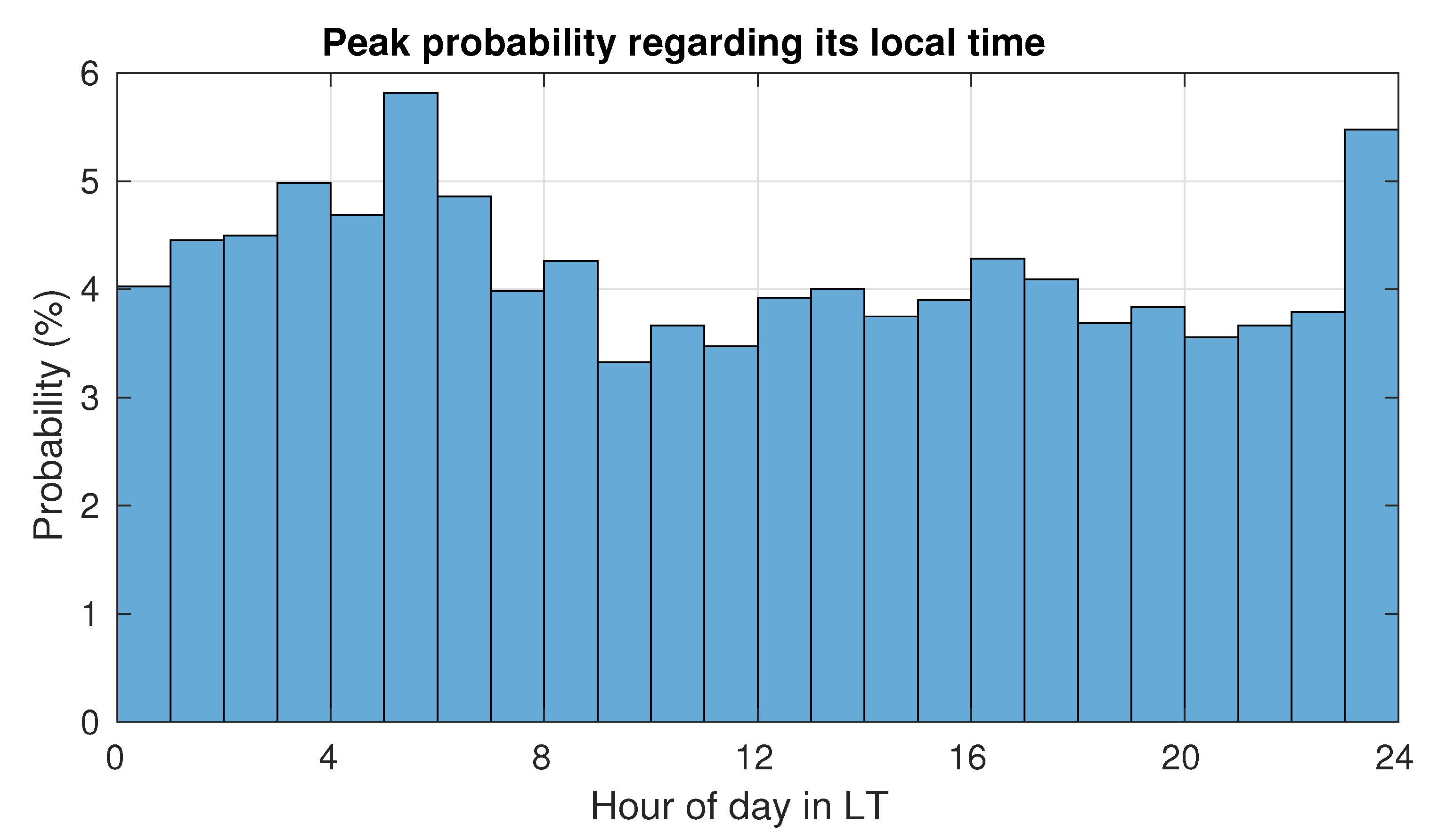
Figure 16.
Histogram of number of events wrt its LT.

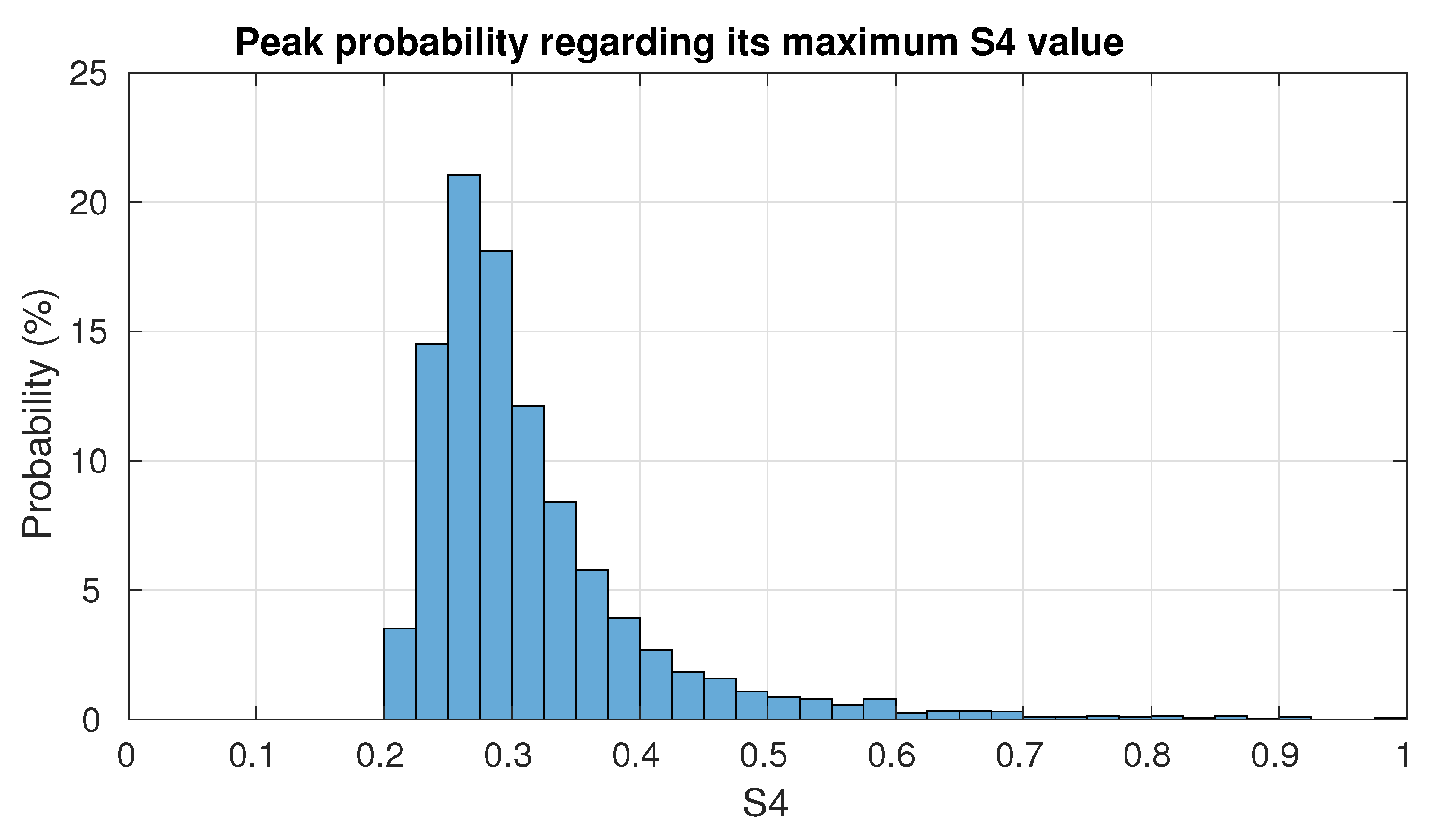
Figure 17.
Histogram of number of events wrt the maximum value reached.

Figure 18.
Histogram count of specular reflection points over all oceans between 40N and 40S) for each S4 value and LT hour, from 0 h to 24 h (UTC) during selected days in 2017.
Figure 18.
Histogram count of specular reflection points over all oceans between 40N and 40S) for each S4 value and LT hour, from 0 h to 24 h (UTC) during selected days in 2017.

Figure 19.
Probability to detect equatorial plasma bubbles (EPBs) with a particular effective time duration, for both years studied in Reference [19]: 2009 (left) during solar minimum and 2014 (right) during the last solar maximum (adapted from Reference [19]).

Figure 20.
Histogram of peak duration during 25 equally spaced days in 2017 representing the probability in bins of 1 s with a total number of samples of around 4700.
Figure 20.
Histogram of peak duration during 25 equally spaced days in 2017 representing the probability in bins of 1 s with a total number of samples of around 4700.

Figure 21.
Histogram of bubble length during 25 equally spaced days in 2017 representing the probability in bins of 5 km with a total number of samples of around 4700.
Figure 21.
Histogram of bubble length during 25 equally spaced days in 2017 representing the probability in bins of 5 km with a total number of samples of around 4700.

Figure 22.
Plasma density (Ne) and Normalized Ne Fluctuation Index for Swarm A during some hours on day 24 August 2017. Note the values of NNeFI when there is fluctuations in the plasma density.
Figure 22.
Plasma density (Ne) and Normalized Ne Fluctuation Index for Swarm A during some hours on day 24 August 2017. Note the values of NNeFI when there is fluctuations in the plasma density.

Figure 23.
Normalized Ne Fluctuation Index for Swarm A, B and C during 24 August 2017 with the predicted mean occurrence of scintillation using WBMOD model. Background image adapted from Reference [20] and overlaid with Swarm data.
Figure 23.
Normalized Ne Fluctuation Index for Swarm A, B and C during 24 August 2017 with the predicted mean occurrence of scintillation using WBMOD model. Background image adapted from Reference [20] and overlaid with Swarm data.

Figure 24.
NNeFI for Swarm A, B and C above 0.05 during day August, along with the peaks above 0.12 detected by CYGNSS during the same day. Note the regions marked with a yellow circle where it can be observed a spatial correlation between both sources of data. Note also, the color scale is shared for and NNeFI.


Table 1.
Summary of CYGNSS mission.
| Parameter | Value |
|---|---|
| Orbital altitude | ∼520 km |
| Inclination | ∼35 |
| Period | 95 min |
| Linear speed | |
| Covered region | 40N to 40S |
| Number of satellites | 8 |
| Number of GNSS satellites tracked per receiver | 4 |
| DDM sample rate | 1 Hz |
| DDM size | (Doppler, delay) |
| DDM Doppler bin resolution | 200 Hz |
| DDM Delay bin resolution | 0.2552 chips |
| Total number of DDMs per day | |
| Dataset volume per day | 10.4 GB |
Table 2.
Table of peaks with larger than 0.2 during more than (or equal to) 5 s on 24 August 2017, in the North Atlantic region.
Table 2.
Table of peaks with larger than 0.2 during more than (or equal to) 5 s on 24 August 2017, in the North Atlantic region.
| Date (dd-mm-yy) | LT | Sat | Ch | Lat (°) | Lon (°) | Duration (s) | Length (km) | Inclination (°) | Max |
|---|---|---|---|---|---|---|---|---|---|
| 24-08-2017 | 4:34 | 1 | 1 | 36.53 | −60.96 | 9 | 67.3 | 29.2 | 0.31 |
| 24-08-2017 | 4:59 | 2 | 1 | 36.63 | −62.13 | 7 | 52.8 | 21.1 | 0.25 |
| 24-08-2017 | 7:05 | 2 | 2 | 35.02 | −34.24 | 6 | 44.1 | 26 | 0.28 |
| 24-08-2017 | 4:21 | 3 | 2 | 34.96 | −50.14 | 6 | 43.8 | 23.8 | 0.27 |
| 24-08-2017 | 4:23 | 3 | 2 | 35.88 | −41.51 | 7 | 52.1 | 17.3 | 0.24 |
| 24-08-2017 | 2:16 | 3 | 3 | 29.71 | −69.37 | 7 | 48 | 10.3 | 0.36 |
| 24-08-2017 | 6:31 | 5 | 1 | 32.88 | −29.54 | 5 | 35.6 | 18 | 0.22 |
| 24-08-2017 | 2:45 | 6 | 1 | 20.66 | −82.03 | 5 | 32 | 53.2 | 0.25 |
| 24-08-2017 | 1:45 | 6 | 2 | 30.04 | −87.14 | 152 | 1044.6 | 50.8 | 0.42 |
| 24-08-2017 | 5:31 | 6 | 3 | 37.27 | −62.21 | 7 | 53.3 | 27.9 | 0.31 |
| 24-08-2017 | 7:14 | 7 | 2 | 33.22 | −29.58 | 7 | 50.1 | 26.6 | 0.26 |
| 24-08-2017 | 2:24 | 7 | 3 | 30.42 | −69.66 | 5 | 34.5 | 12.1 | 0.37 |
| 24-08-2017 | 2:22 | 7 | 4 | 19.67 | −76.12 | 62 | 396.2 | 59.5 | 0.45 |
| 24-08-2017 | 3:56 | 8 | 1 | 34.56 | −61.95 | 7 | 51.1 | 18.6 | 0.32 |
| 24-08-2017 | 1:50 | 8 | 2 | 30.05 | −86.84 | 144 | 988.1 | 48.8 | 0.54 |
| 24-08-2017 | 6:02 | 8 | 3 | 34.94 | −34.41 | 7 | 51.3 | 13.7 | 0.31 |
| 24-08-2017 | 2:50 | 8 | 4 | 21.28 | −81.78 | 76 | 490.4 | 51.3 | 0.57 |
Table 3.
Table of peaks with higher than 0.2 during more than (or equal to) 5 s on 20 May 2019, at Indian Ocean.
Table 3.
Table of peaks with higher than 0.2 during more than (or equal to) 5 s on 20 May 2019, at Indian Ocean.
| Date (dd-mm-yy) | LT | Sat | Ch | Lat (°) | Lon (°) | Duration (s) | Length (km) | Inclination (°) | Max |
|---|---|---|---|---|---|---|---|---|---|
| 20-05-2019 | 19:05 | 1 | 3 | −1.25 | 58.34 | 7 | 42.6 | 39.9 | 0.32 |
| 20-05-2019 | 06:08 | 1 | 3 | −16.87 | 121.40 | 6 | 37.7 | 58.7 | 0.28 |
| 20-05-2019 | 08:59 | 2 | 1 | 15.00 | 41.64 | 325 | 2069.9 | 14.5 | 0.51 |
| 20-05-2019 | 16:40 | 2 | 1 | 17.24 | 111.29 | 11 | 68.7 | 33.3 | 0.47 |
| 20-05-2019 | 08:21 | 2 | 2 | 6.79 | 55.99 | 6 | 36.2 | 27.1 | 0.28 |
| 20-05-2019 | 09:00 | 2 | 3 | 18.41 | 40.30 | 245 | 1555.9 | 33.7 | 0.41 |
| 20-05-2019 | 08:21 | 2 | 4 | 2.89 | 58.37 | 6 | 36.0 | 59.3 | 0.27 |
| 20-05-2019 | 17:18 | 2 | 4 | 11.00 | 97.45 | 65 | 396.6 | 20.0 | 0.63 |
| 20-05-2019 | 17:30 | 4 | 1 | 8.86 | 97.49 | 146 | 881.6 | 20.2 | 0.27 |
| 20-05-2019 | 07:55 | 4 | 3 | 7.04 | 74.61 | 8 | 48.2 | 16.3 | 0.32 |
| 20-05-2019 | 08:32 | 4 | 3 | 9.07 | 56.36 | 7 | 42.4 | 33.1 | 0.33 |
| 20-05-2019 | 16:59 | 4 | 3 | 12.92 | 53.16 | 27 | 166.9 | 66.0 | 0.26 |
| 20-05-2019 | 08:05 | 5 | 2 | 13.69 | 97.45 | 192 | 1186.6 | 25.4 | 0.74 |
| 20-05-2019 | 08:39 | 5 | 2 | 9.66 | 75.84 | 106 | 645.0 | 36.3 | 0.52 |
| 20-05-2019 | 09:15 | 5 | 2 | 11.98 | 52.58 | 38 | 235.0 | 22.9 | 0.35 |
| 20-05-2019 | 07:35 | 5 | 3 | 3.05 | 57.99 | 6 | 36.2 | 34.2 | 0.30 |
| 20-05-2019 | 09:16 | 5 | 3 | 9.80 | 56.21 | 6 | 36.4 | 53.2 | 0.29 |
| 20-05-2019 | 17:06 | 5 | 4 | 12.01 | 71.56 | 20 | 126.0 | 68.3 | 0.34 |
| 20-05-2019 | 07:09 | 6 | 3 | 5.67 | 73.95 | 9 | 53.9 | 52.4 | 0.27 |
| 20-05-2019 | 18:48 | 6 | 3 | 7.98 | 116.57 | 32 | 197.5 | 37.3 | 0.48 |
| 20-05-2019 | 09:16 | 6 | 4 | 7.13 | 98.00 | 53 | 326.0 | 65.4 | 0.28 |
| 20-05-2019 | 07:45 | 6 | 4 | 0.33 | 57.62 | 6 | 35.6 | 45.6 | 0.30 |
| 20-05-2019 | 17:13 | 7 | 2 | 16.22 | 112.29 | 12 | 75.5 | 38.1 | 0.36 |
| 20-05-2019 | 08:17 | 7 | 3 | 6.87 | 75.01 | 6 | 36.7 | 49.5 | 0.29 |
| 20-05-2019 | 08:43 | 8 | 2 | 16.92 | 41.11 | 265 | 1673.2 | 41.9 | 0.23 |
Publisher’s Note: MDPI stays neutral with regard to jurisdictional claims in published maps and institutional affiliations. |
© 2020 by the authors. Licensee MDPI, Basel, Switzerland. This article is an open access article distributed under the terms and conditions of the Creative Commons Attribution (CC BY) license (http://creativecommons.org/licenses/by/4.0/).
Share and Cite
MDPI and ACS Style
Molina, C.; Camps, A. First Evidences of Ionospheric Plasma Depletions Observations Using GNSS-R Data from CYGNSS. Remote Sens. 2020, 12, 3782. https://0-doi-org.brum.beds.ac.uk/10.3390/rs12223782
AMA Style
Molina C, Camps A. First Evidences of Ionospheric Plasma Depletions Observations Using GNSS-R Data from CYGNSS. Remote Sensing. 2020; 12(22):3782. https://0-doi-org.brum.beds.ac.uk/10.3390/rs12223782
Chicago/Turabian StyleMolina, Carlos, and Adriano Camps. 2020. "First Evidences of Ionospheric Plasma Depletions Observations Using GNSS-R Data from CYGNSS" Remote Sensing 12, no. 22: 3782. https://0-doi-org.brum.beds.ac.uk/10.3390/rs12223782
Note that from the first issue of 2016, this journal uses article numbers instead of page numbers. See further details here.