1. Introduction
Soybean (
Glycine max L. Merrill) diseases can have a significant impact on production and profits [
1]. During the years from 2015 to 2019, soybean diseases were responsible for losses of around 8.99% of the production potential in the U.S., which equates to an average of USD 3.8 billion annually [
2]. Sudden death syndrome (SDS) is one of the most damaging soybean diseases found throughout most of the soybean production area in the United States. SDS is caused by a soilborne fungus
Fusarium virguliforme (
Fv) that causes root rot and foliar symptoms that typically become visible during reproductive stages [
3]. Visual assessment of SDS requires intensive crop scouting that is time-consuming and labor-intensive. Therefore, an automated method for the detection of SDS is necessary.
Timely detection and management of plant diseases are essential for reducing yield loss. Remote sensing technology has proven to be a practical, noninvasive tool for monitoring crop growth and assessing plant health [
4,
5]. Sensing instruments can record radiation in various parts of the electromagnetic spectrum, including ultraviolet, visible, near-infrared (NIR) and thermal infrared, to name a few [
6]. Healthy and diseased plant canopies absorb and reflect incident sunlight differently due to changes in leaf and canopy morphology and chemical constituents [
7,
8]. These changes can alter the optical spectra, such as a decrease in canopy reflectance in the near-infrared band and an increase in reflectance in the red band [
7]. Some widely used methods include thermography [
9,
10,
11], fluorescence measurements [
12,
13,
14] and hyperspectral techniques [
15,
16,
17].
In the past few years, several studies have been conducted for the detection of plant diseases [
18,
19,
20]. For example, Durmus et al. [
18] used red, green and blue (RGB) cameras for disease-detection on tomato leaves. In another study, Gold et al. [
19] used lab-based spectroscopy to detect and differentiate late and early blight diseases on potato leaves. Specific to SDS, Bajwa et al. [
21] and Herrmann et al. [
3] used handheld and tractor-mounted sensors, respectively, for SDS detection. These successful applications help ease the demand for expert resources and reduce the human errors in the visual assessment and, eventually, management of plant diseases.
However, most of these methods are near-sensing techniques that focus on individual plants. In practice, it is more reasonable and efficient to diagnose plant diseases such as SDS from the quadrat level. There are several options for collecting imagery for the detection of plant diseases at the quadrat level, including unmanned aerial vehicles (UAV) [
22,
23], tractor-mounted tools [
3] and satellite imagery [
24]. Satellite imagery is typically less expensive, covers a wide ground swath and can provide temporal flexibility because the fields can be continuously monitored non-destructively. The frequency of image collection is determined by the number of satellites that pass that field [
25]. Although the imagery from UAVs and tractor-mounted tools is often higher resolution at the quadrat level, these tools are cumbersome for farmers to operate and maintain in a commercial system and often lack spatial information. Satellite imagery, on the other hand, contains spatial information, comes preprocessed and continuously improves in resolution.
In addition to quality data, efficient and accurate analysis of the sensor data is essential for accurate detection of plant diseases. For the analysis of visible sensing information, several machine learning methods have been used. Common methods that have been used in plant disease diagnosis using images are convolutional neural networks (CNNs) and random forest. Different from full connected neural networks, CNNs have two special layer types. The convolutional layers extract features from the input images. The pooling layers reduce the dimensionality of the features. Dhakate et al. [
26] used a CNN for the recognition of pomegranate diseases with 90% overall accuracy. Ferentinos [
27] developed CNN models to classify the healthy and diseased plants with 99.5% success. Polders et al. [
28] used fully convolutional neural networks to detect potato virus in seed potatoes. However, in our case, the resolution of satellite imagery was 3 m × 3 m, which means the satellite imagery of each generalized quadrat only contained several pixels. CNNs or other methods are less suitable for this task. How to deal with low-pixel-level remote sensing data is important for improving classification accuracy. Random forest was also used for disease detection and classification [
29]. Samajpati et al. [
30] used a random forest classifier to classify different apple fruit diseases. Chaudhary et al. [
31] proposed an improved random forest method, which achieved 97.8% for a multi-class groundnut disease dataset. Although random forest is popular for its easy implementation and high efficiency on large datasets, its performance is influenced by the hyperparameter choices, such as random seeds and the number of variables [
32].
Most of the current plant disease identification methods use field images at a single time-point to identify the contemporary status of the disease. The use of temporal image sequences can help improve detection accuracy. For example, a recurrent neural network (RNN) was designed for solving the multivariate time-series prediction problem [
33]. However, RNN is faced with gradient vanishing/exploding problems [
34]. As an improved version of RNN, the long short-term memory model (LSTM) is used for its successful application to natural language modeling [
35]. Compared with RNN, LSTM has more gates that can control the reset of the memory and the update of the hidden states. Turkoglu et al. [
36] proposed an LSTM-based CNN for the detection of apple diseases and pests, which scored 96.1%. Namin et al. [
37] utilized a CNN-LSTM framework for plant classification of various genotypes as well as the prediction of plant growth and achieved an accuracy of 93%. Navarro et al. [
38] proposed an LSTM method for the prediction of low temperatures in agriculture and obtained a determination coefficient (accuracy) of 99%. Although LSTM has alleviated the gradient vanishing/exploding problem of RNNs, the training speed of LSTM is much slower due to the increased number of parameters. To solve this issue, Chung et al. [
39] introduced the gated recurrent unit (GRU) in 2014. Since GRU only has two gates (i.e., reset gate and update gate) and uses the hidden state to transfer information, its training speed is much faster. Jin et al. [
40] used a deep neural network which combined CNN and GRU to classify wheat hyperspectral pixels and obtained an accuracy of 0.743.
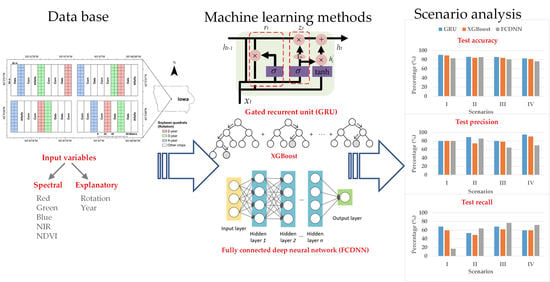
The objective of this paper is to detect SDS in soybean quadrats using 3m x 3m resolution satellite imagery which contains RGB and NIR information. The GRU-based model was compared in different scenarios (i.e., percentage of diseased quadrats) to the most popular neural network and tree-based methods, namely, a fully connected deep neural network (FCDNN) and XGBoost.
This paper is organized as follows.
Section 2 introduces the dataset and methods used.
Section 3 includes a case study, the calculation results and comparisons of the three methods. The paper concludes with the summary, findings and future research directions in
Section 4.
2. Materials and Methods
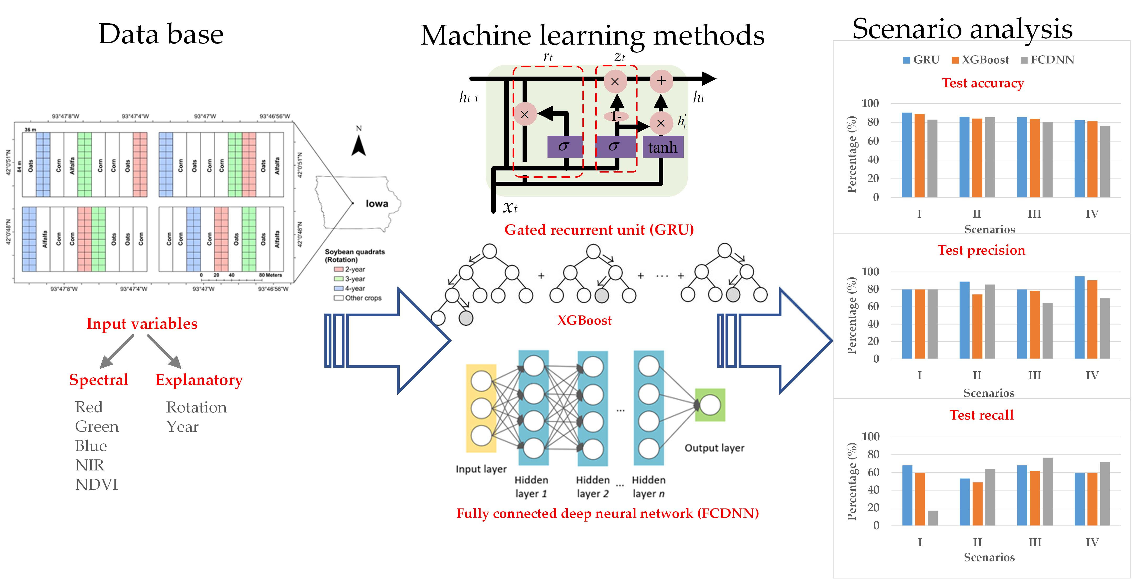
Data were collected in 2016 and 2017 from an ongoing soybean field experiment located at the Iowa State University Marsden Farm, in Boone County, Iowa (
Figure 1) [
29,
41,
42,
43]. This study site was chosen because soybean plots in this experiment have consistently displayed a range of SDS levels since 2010 [
44]. In the trial site, there were three cropping systems, 2-year, 3-year and 4-year crop rotations, which are represented by using one-hot encoding, i.e., “100”, “010” and “001”, respectively. In the 2-year cropping rotation, corn and soybean were planted in rotation with synthetic fertilizers at the conventional rate. In the 3-year cropping rotation, corn, soybean, oat and red clover were planted in rotation with composted cattle manure and synthetic fertilizers at reduced rates. In the 4-year cropping rotation, corn, soybean, oat and alfalfa were planted in rotation with composted cattle manure and synthetic fertilizers at reduced rates. More information about the experiment can be found in these studies [
29,
41,
42,
43]. In each year, 240 soybean quadrats (3 m wide × 1.5 m long) were marked to collect disease data. The soybean variety (Latham L2758 R2, maturity group 2.7) remained the same for all seasons.
2.1. Data Processing
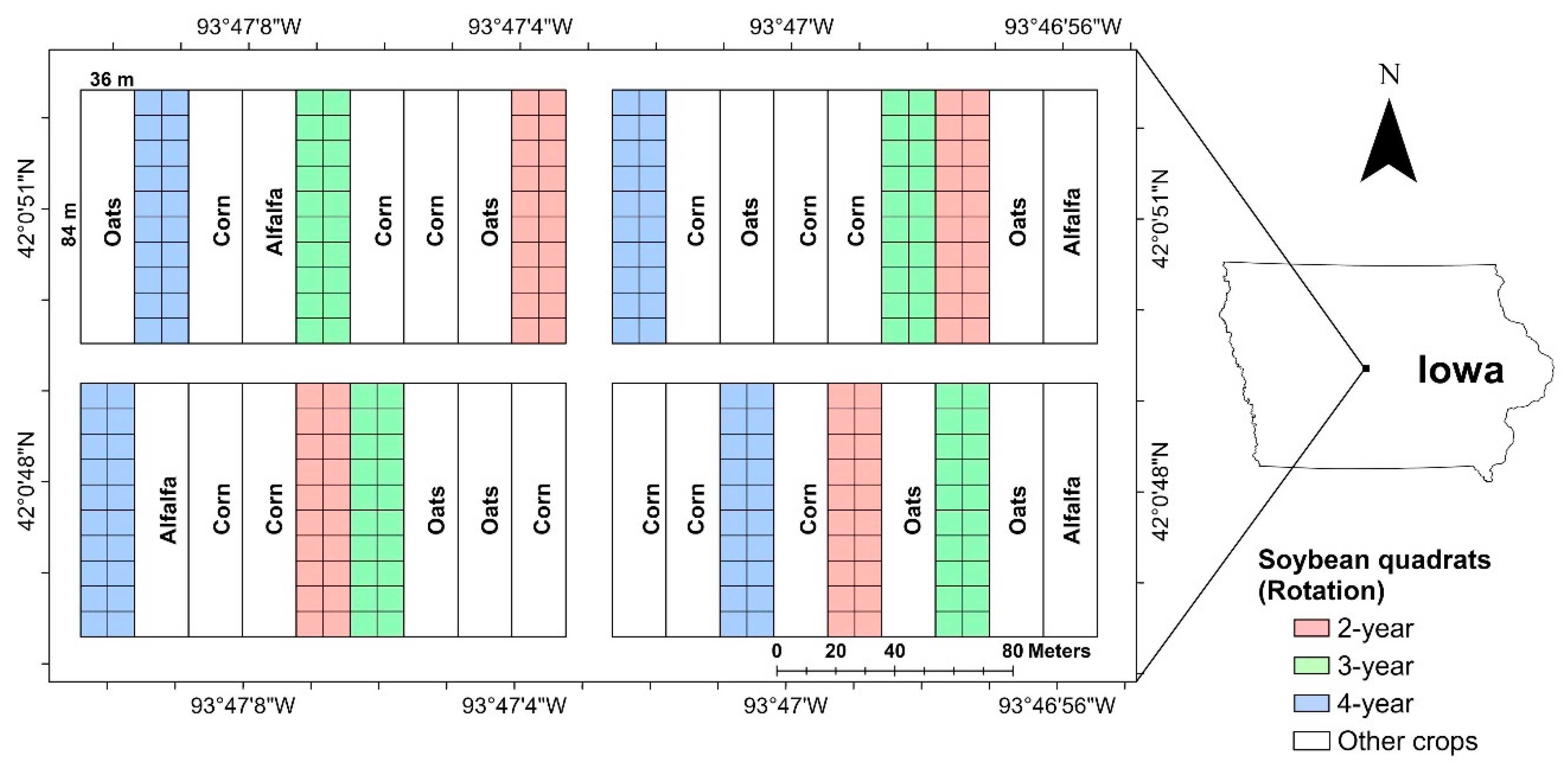
Figure 2 illustrates our method for data collection, data processing and analysis for the detection of SDS in this study. This methodology has been explained in detail.
Satellite images were collected on 5 July 2016, 9 July 2016, 20 July 2016, 5 August 2016, 21 August 2016, 31 August 2016, 5 July 2017, 9 July 2017, 20 July 2017, 2 August 2017, 18 August 2017 and 23 August 2017. In addition to spectral information, the dataset also included ground-based crop rotation information that is an explanatory variable. The data source of satellite imagery is PlanetScope (
https://www.planet.com/) satellite operated by Planet Labs (San Francisco, CA), a private imaging company. PlanetScope satellite imagery comes with four bands, including red (590–670 nm), green (500–590 nm), blue (455–515 nm) and NIR (780–860 nm). Soybean quadrats were generalized to large quadrats (8.6 mW × 9.1 mL) for data extraction from images and subsequent data analysis. As such, the imagery of each quadrat has 6–9 pixels.
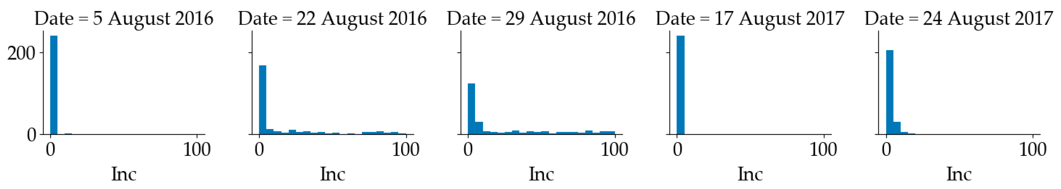
The number of total plants and plants showing foliar symptoms of SDS was counted in each quadrat to calculate the disease incidence on a 0 to 100% scale, based on the percentage of diseased plants. The distribution of SDS incidence is shown in
Figure 3. It can be observed that in 2016, SDS incidence in more than half of the 240 quadrats was less than 5% and the SDS incidence of the rest quadrats ranged from 5% to 100%. In 2017, the SDS incidence of most quadrats was below 5%. In this paper, if a quadrat had an SDS incidence above 5%, it was considered as diseased (positive); otherwise, it was considered as healthy (negative). The inspection dates used for the analysis were 27 July 2016, 5 August 2016, 22 August 2016 and 29 August 2016. Since the visual disease scores on 27 July 2016 were all zeros, all the imagery collected before that date was labeled as healthy. The human visual ratings recorded on 5 August 2016 were mapped to the imagery collected on the same date. The visual score on 22 August 2016 was mapped to the imagery collected on 21 August 2016, while the SDS rating recorded on 31 August 2016 was mapped to the imagery collected on 29 August 2016 Similarly, in 2017, the human visual ratings recorded on 17 August 2017 were mapped to the imagery collected on 18 Aug and the human visual ratings recorded on 24 August 2017 were mapped to the imagery collected on 23 August 2017. There was only one diseased quadrat on 5 August 2016. In 2016, all quadrats were healthy before 5 August 2016. In 2017, all quadrats were healthy before 17 August 2017. The aim was to determine whether the quadrat had SDS or not.
The mean and variance of the normalized RGB, normalized difference vegetation index (NDVI) and NIR information of each quadrat were used as predictors for two reasons. First, the number of pixels varied from quadrat to quadrat. Second, the SDS rating represented the entire quadrat. Some information could be lost if each pixel were used separately. The crop rotation information was used as a categorical variable encoded by one-hot method. Therefore, there were a total of 12 variables for each quadrat, which included the year, crop rotation, the mean values and the variance values of RGB and NIR bands and NDVI. The NDVI is calculated as Equation (1).
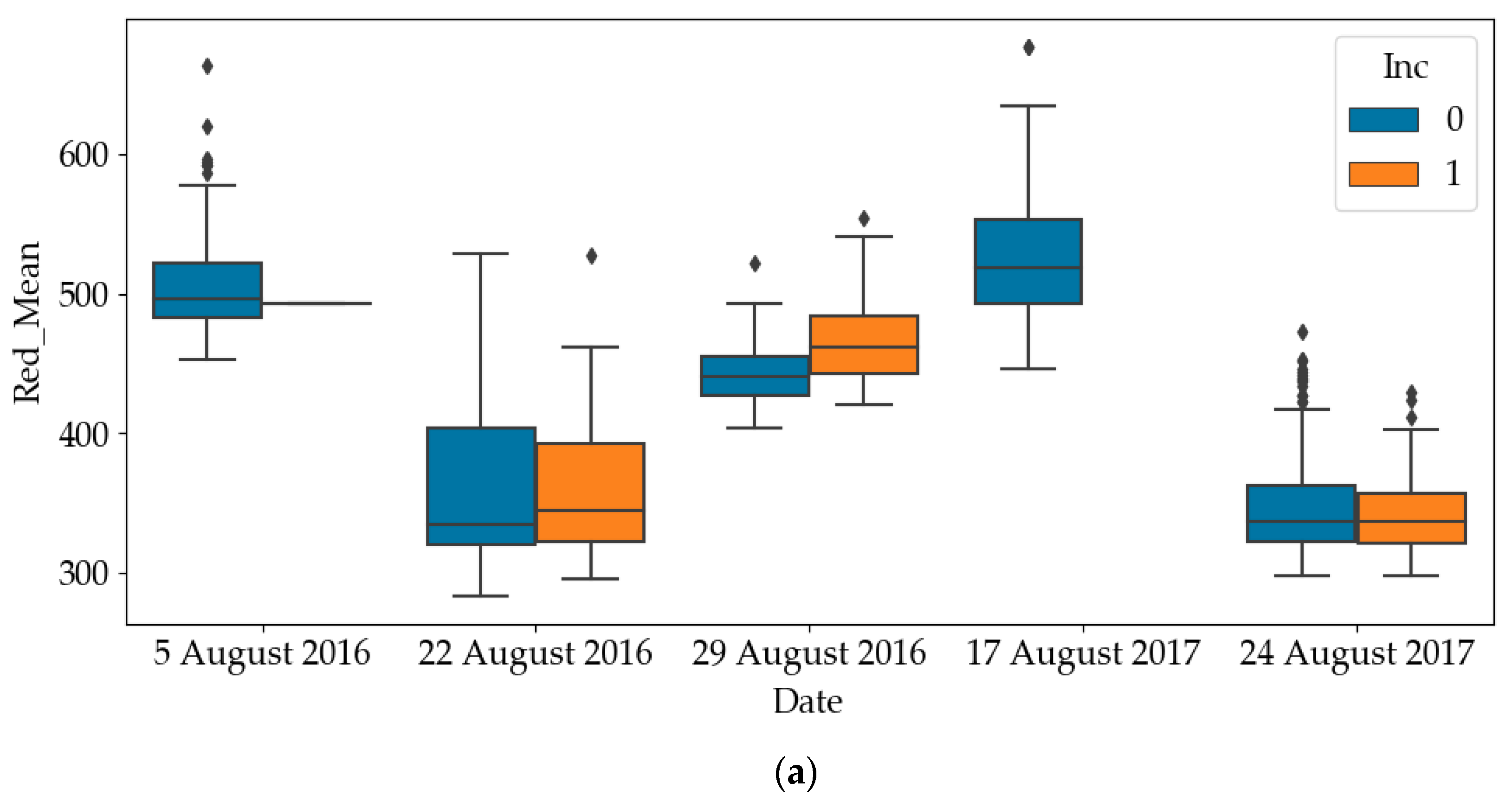
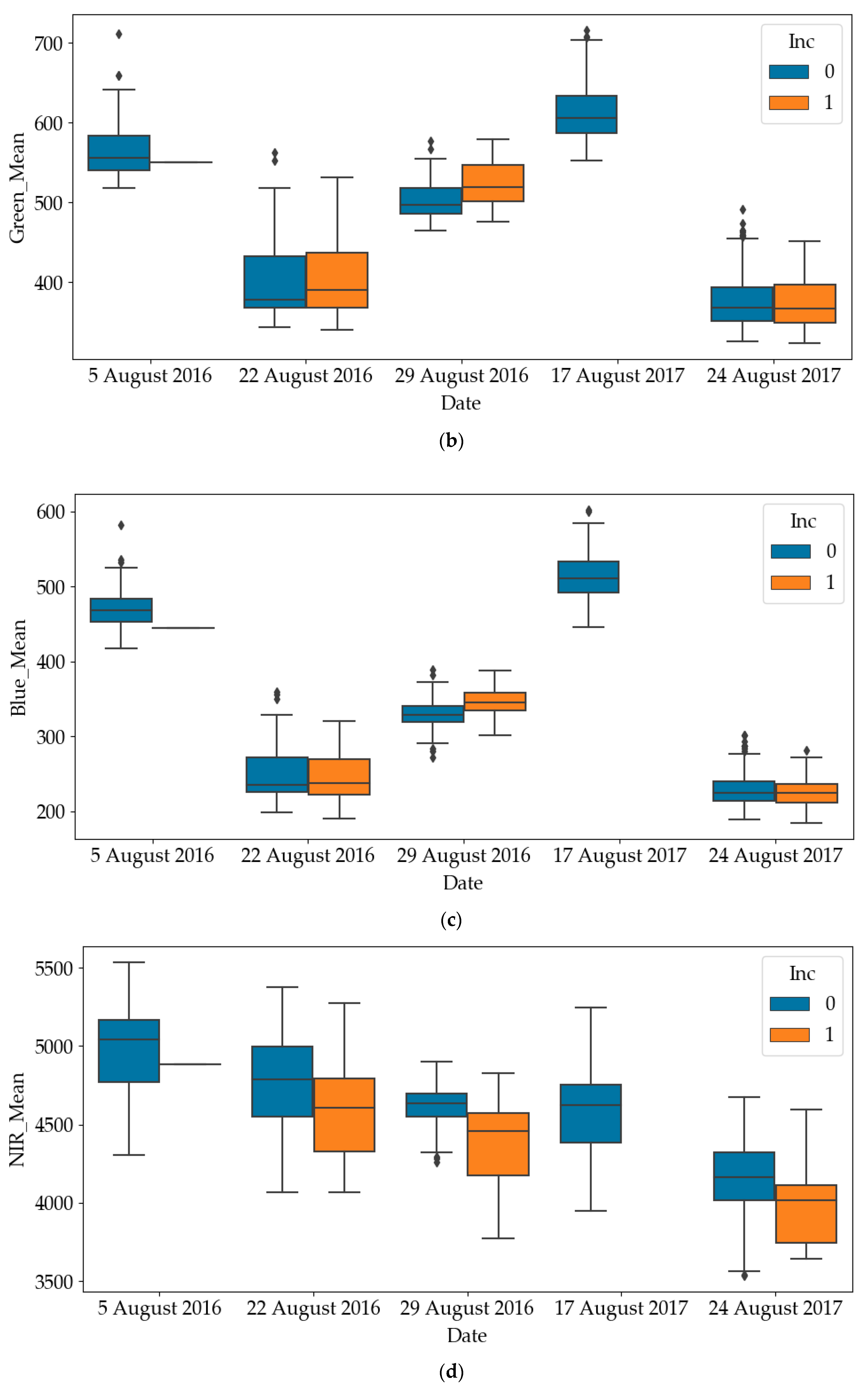
The box plots of RGB and NIR of diseased quadrats and healthy quadrats are shown in
Figure 4. Since all quadrates were healthy on the other dates, only the results on later dates have been plotted. It can be noticed that the RGB values of diseased quadrats were lower than those of healthy quadrats, while the NIR values of diseased quadrats were greater than those of healthy quadrats. This indicates that SDS does influence light emissions of leaves. As such, one of the objectives of this paper is to use these predictors to detect the SDS-infected quadrats. To avoid mutual interference between data samples collected in a quadrat at different time points, the dataset was divided into a training and a testing dataset according to quadrat number. For the experiment in each year, we randomly selected 200 quadrats (83% of the dataset) as the training dataset and 40 quadrats (17% of the dataset) as the testing dataset of the total 240 quadrats.
2.2. Measurements
Three indices, including overall accuracy, precision and recall, as calculated in Equations (2)–(4), were measured to evaluate the performance of models. The definitions of true positive (TP), true negative (TN), false positive (FP) and false negative (FN) are shown in
Table 1.
2.3. Methods
Three methods were investigated in this paper. The first is the GRU-based method. The second is XGBoost, which is the representative of tree-based methods. The third is an FCDNN, which is the most widely used deep learning method. As for comparisons, both XGBoost and the FCDNN used individual images while the GRU-based method used time-series images.
2.3.1. Gated Recurrent Unit (GRU)-Based Method
Most of the existing methods use one individual spectral measurement to predict the corresponding SDS [
3]. Nevertheless, the multiple images at different times of the same quadrat may help improve the prediction accuracy of the model. Thus, a method that can handle time-series imagery is needed. Recurrent neural networks (RNNs) are suitable for non-linear time-series processing [
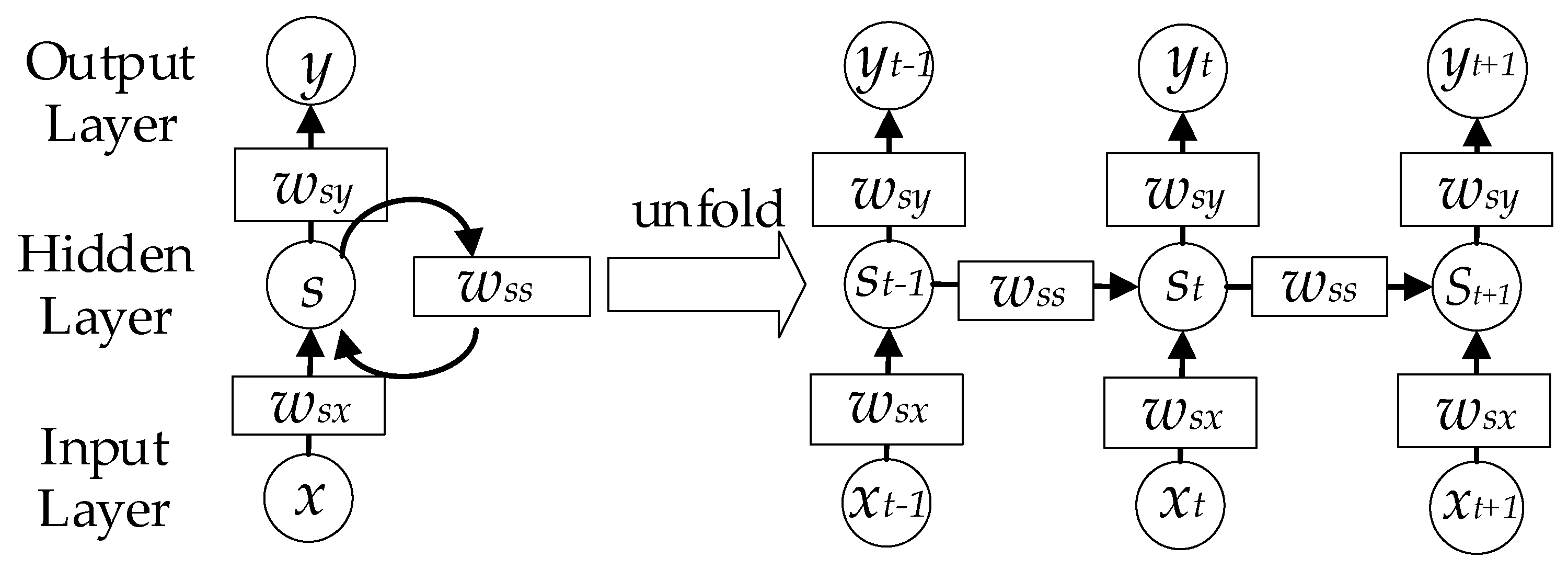
45]. As shown in
Figure 5, the RNN consists of an input layer
x, a hidden layer
h and an output layer
y. When dealing with time-series data, the RNN can be unfolded as the right part. The output and hidden layers can be calculated according to Equation (5) and Equation (6), respectively.
Despite its popularity as a universal function approximator and easy implementation, the RNN method is faced with the gradient vanishing/exploding problem. In the training process of RNNs, gradients are calculated from the output layer to the first layer of the RNN. If the gradients are smaller than 1, the gradients of the first several layers will become small through many multiplications. On the contrary, the gradients will become very large if the gradients are larger than 1. Therefore, it sometimes causes the gradients to become almost zero or very large when it reaches the first layers of RNNs. Consequently, the weights of the first layers will not get updated in the training process. Therefore, simple RNNs may not be suitable for some complex problems.
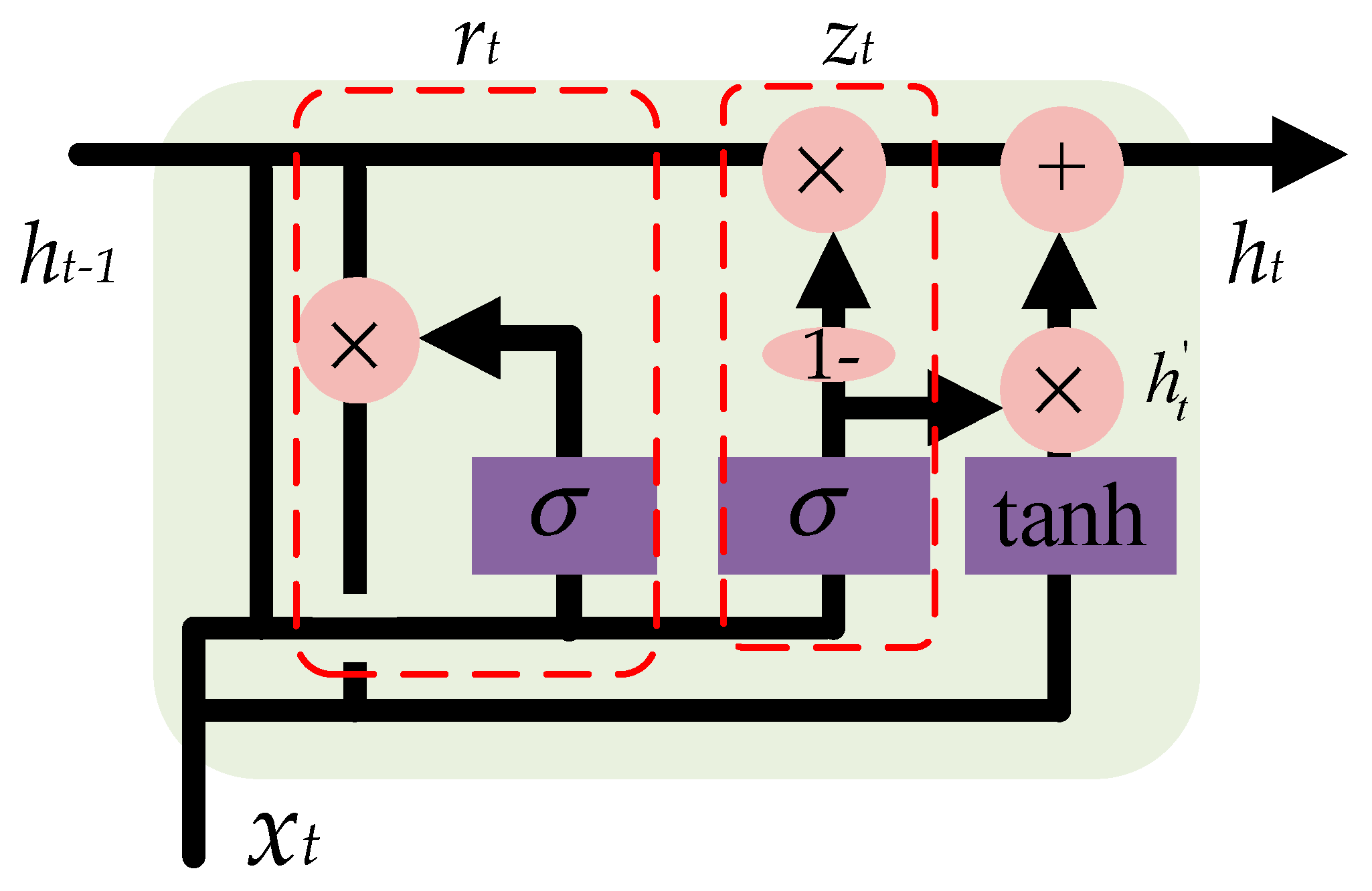
In this paper, a GRU-based method is proposed to deal with the multivariate time-series imagery data that will solve the vanishing gradient problem of a standard RNN [
39]. As shown in
Figure 6, based on the previous output
ht−1 and the current input
xt, a reset gate is used to determine which part of information should be reset, as calculated in Equation (7), while an update gate is used to update the output of the GRU
ht, as calculated in Equation (8). The candidate hidden layer is calculated according to Equation (9). The current output can be obtained according to Equation (10). The gates, namely,
zt and
rt, and parameters, namely,
Wz,
Wr and
W, of the GRU were updated in the training process.
2.3.2. Fully Connected Deep Neural Network (FCDNN)
FCDNN is a class of methods that use multiple layers to extract information from the input data [
46]. The basic layers are a fully connected layer and an activation layer. The fully connected layer consists of multiple neurons. Each neuron in a fully connected layer connects to all neurons in the next layer. The output of a fully connected layer is calculated as Equation (11).
The fully connected layer can only deal with a linear problem. To add the non-linear characteristic to the model, the concept of activation layers was introduced. Some widely used activation functions include sigmoid function, hyperbolic tangent function (Tanh) and rectified linear unit (ReLU) function. In this paper, ReLU is used as Equation (12).
The loss function is used to measure the performance of models. In this paper, binary cross-entropy loss function is used, which can be calculated as Equation (13),
where
N is the total number of the samples,
i is the index of the sample,
yi is the label of the
ith sample and
p(
yi) is the predicted probability of the sample belonging to the class.
The most common training method is stochastic gradient descent which calculates the gradients and then updates the weights and biases iteratively. The final goal of training is to minimize the loss function. FCDNNs can deal with large datasets and execute feature engineering without explicit programming.
2.3.3. XGBoost
The XGBoost method is a popular tree-based method for classification tasks [
47]. A decision tree consists of three parts: branches, internal nodes and leaf nodes. The internal nodes are a set of conditions that can divide the samples into different classes. The branches represent the outcome of internal nodes. The leaf nodes represent the label of the class. A decision-tree can break down a complex classification problem into a set of simpler decisions at each stage [
48].
One of the most famous tree-based methods is random forest. Random forest is an ensemble method that grows many trees and outputs the class based on the results of each individual tree. Given a training set
X with labels
Y, it randomly selects samples with replacement of the training set and train the trees,
b1,
b2,
b3, …,
bB. After training, for sample
x’, the prediction can be made by averaging the predictions of each tree or using the majority voting method. Since the bootstrap sampling method can reduce the variance of the model without increasing the bias, the model can have better generalization performance. Since each tree is trained separately, it can be implemented in parallel, which can save a lot of time. Another merit of random forest is that it can deal with high-dimensional dataset and identify the importance of each variable. Different from a random forest algorithm, which generates many trees at the same time, XGBoost is trained in an additive manner. In each iteration of XGBoost training, a new decision tree that minimizes the prediction error of previous trees will be added to the model. The prediction of a sample can be calculated by summarizing the scores of each tree. XGBoost also includes a regularization term in the loss function, which can further improve the generalization ability of the model. The specific details are given in [
47].
3. Results
To validate the proposed technique, numerical calculations were conducted. The Python code can be found in the
Supplementary Materials.
3.1. Model Parameters
The FCDNN consists of six fully connected layers which include 12, 8, 8, 8, 4 and 1 neurons, respectively. After each fully connected layer, a ReLU layer and a dropout layer are included. The dropout rate is 0.2. The binary cross-entropy function is used as the loss function of the model. The optimizer is stochastic gradient descent. To avoid overfitting, the dropout technique was also used for each fully connected layer. The learning rate was set as 0.008. The batch size was 100. The maximum number of iterations was set to 300.
For XGBoost, the max number of leaves was set as 40. The max depth was set as 10. The objective is the binary cross-entropy function. The maximum number of iterations was 300.
For the proposed model, two GRU layers were stacked. The first GRU layer coverts each input sequence to a sequence of 50 units. Then, the second GRU layer converts the sequences of 50 units to sequences of 25 units. Then, a fully connected layer is used to transform the 25 variables to one output. The learning rate was set as 0.012. The batch size was 100. The maximum number of iterations was set to 300. All three models used the cross-entropy loss function as Equation (13).
3.2. Calculations in Different Scenarios
To determine the effectiveness of the GRU-based method in different scenarios (i.e., the percentage of diseased quadrats), four analyses have been conducted. Since both the dataset of 2016 and that of 2017 had six pairs of imagery and human visual ratings, the dates of each year were numbered from 1 to 6. All the soybean plants at time points 1 to 3 in 2016 and time points 1 to 4 in 2017 were healthy; therefore, to reduce the influence of imbalanced data, we targeted to predict SDS at time points 3 to 6 in 2016 and 5 to 6 in 2017.
The specific settings of each calculation are shown in
Table 2. In calculation I, the target was to predict SDS at time points 3 to 6 in 2016 and time points 5 and 6 in 2017. In the training of the GRU-based model, the imagery collected at time points 1 and 2 was added to construct the time-series imagery samples. The sequence length was set as three. Thus, four sequences of satellite imagery (i.e., 1-2-3, 2-3-4, 3-4-5 and 4-5-6) can be generated for each quadrat in the experiment of 2016 and two sequences of satellite imagery (i.e., 3-4-5 and 4-5-6) can be generated for each quadrat in the experiment of 2017. In the training of XGBoost and the FCDNN, only labeled satellite imagery at time points 3, 4, 5 and 6 was used to train the model. For the three methods, since there were 200 quadrats for training and 40 quadrats for testing in each year, the number of training samples was 1200 (200 × 6) and the number of testing samples was 240 (40 × 6).
In calculation II, the target was SDS at the time points 4, 5 and 6 in 2016 and time points 5 and 6 in 2017. In the training of the GRU-based model, the sequence length was set as four. Thus, three sequences of satellite imagery (i.e., 1-2-3-4, 2-3-4-5 and 3-4-5-6) can be generated for each quadrat in the experiment of 2016 and two sequences of satellite imagery (i.e., 2-3-4-5 and 3-4-5-6) can be generated for each quadrat in the experiment of 2017. The number of training samples was 1000 (200 × 5) and the number of testing samples was 200 (40 × 5).
In calculation III, the target was SDS at the time points 5 and 6 in 2016 and time points 5 and 6 in 2017. In the training of the GRU-based model, the sequence length was set as five. Thus, two sequences of satellite imagery (i.e., 1-2-3-4-5 and 2-3-4-5-6) can be generated for each quadrat in the experiment of 2016 and two sequences of satellite imagery (i.e., 1-2-3-4-5 and 2-3-4-5-6) can be generated for each quadrat in the experiment of 2017. The number of training samples was 800 (200 × 4) and the number of testing samples was 160 (40 × 4).
In calculation IV, the target was SDS at the time point 6 in 2016 and time point 6 in 2017. In the training of the GRU-based model, the sequence length was set as six. Thus, one sequence of satellite imagery (i.e., 1-2-3-4-5-6) can be generated for each quadrat in the experiment of 2016 and one sequence of satellite imagery (i.e., 1-2-3-4-5-6) can be generated for each quadrat in the experiment of 2017. The number of training samples was 400 (200 × 2) and the number of testing samples was 80 (40 × 2).
The results are shown in
Table 3. In calculation I, the three methods had the same test precision. However, the test recall of GRU was 9% and 51% greater than that of XGBoost and the FCDNN, respectively. The reason why the test recall of the FCDNN is much less is that the model was overfitted and most of the samples were predicted as healthy. In calculation II, the test accuracy of GRU was 2% greater than that of XGBoost and 0.5% greater than that of the FCDNN owing to the improved test precision. It means that most of the positive predictions were accurate. In calculation III, the test accuracy of GRU was 1.8% and 5% greater than that of XGBoost and the FCDNN, respectively. In calculation IV, the test accuracy of GRU was 1.2% and 6% greater than that of XGBoost and the FCDNN, respectively. It can be observed that the training accuracy of GRU was lower in the four calculations; however, the test accuracy of GRU is the highest among the three methods in the four calculations. It proves the good generalization performance of the GRU-based method. The test precision of GRU was highest in the four calculations, which was about 80–95%. In terms of test recall, the FCDNN outperformed the other two methods in calculations II, III and IV. However, its test accuracy was lower because the proportion of positives that are correctly identified was lower.
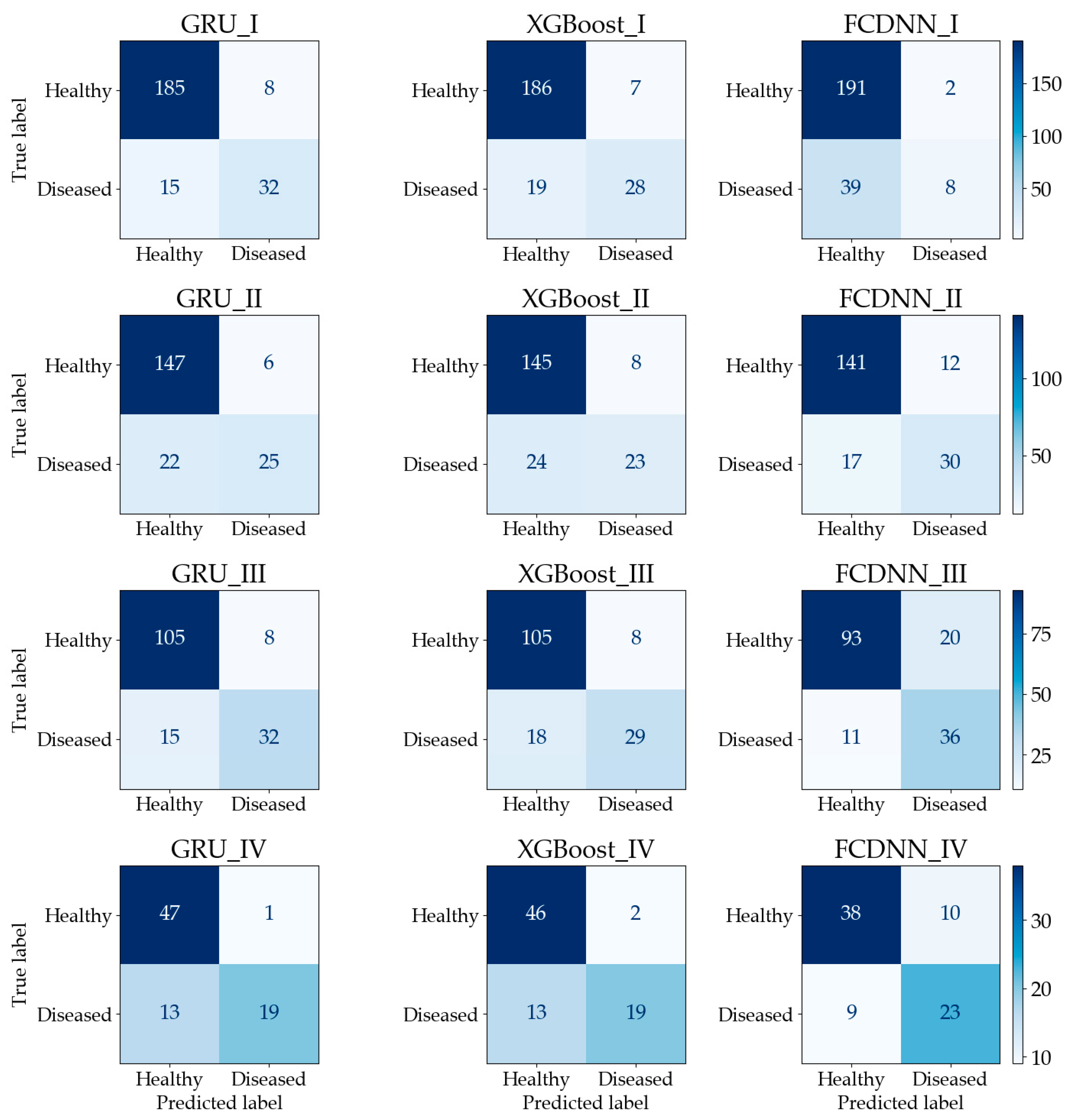
The confusion matrices are shown in
Figure 7. In calculation I, although GRU has the lowest number of true predictions for healthy quadrats, it has more true predictions for diseased quadrats than the other two methods. For the FCDNN, the opposite is the case, since 230 quadrats were classified as healthy and only 10 quadrats were classified as diseased. The reason is that the FCDNN is more likely to predict samples as healthy. In calculation II, GRU made more true predictions for healthy quadrats. In calculation III, Both GRU and XGBoost classified 105 healthy quadrats correctly; however, GRU had more true predictions for diseased quadrats than XGBoost. In calculation IV, the performance of GRU was similar to that of XGBoost; the difference was only one healthy quadrat. The FCDNN did not perform well in the classification of healthy quadrats. In conclusion, the calculation results show that prediction accuracy can be improved by using a sequence-based model, i.e., GRU, with time-series imagery.
3.3. Data Imbalance
The number of healthy samples was much larger than that of diseased samples (
Table 2). This is a typical example of a data imbalance issue. One possible consequence is that the learning models will be guided by global performance, while the minority samples may be treated as noise [
49]. For example, for a dataset consisting of 90 negative examples and 10 positive samples, a classifier that predicts all samples to be positive can achieve an overall accuracy of 90%. However, the classifier does not have the ability to predict positive examples. In our case, the training processes of the models were guided by the cross-entropy loss function. To reduce the loss, models were more likely to predict the samples as healthy since healthy samples were the majority. This pattern can be observed from the results shown in
Table 3. In most of the situations, the test precision was 10–20% greater than the test recall. There are two common approaches to address the issue of data imbalance. One way is to eliminate the data imbalance by using sampling methods [
50]. Over-sampling methods create more new minority classes while under-sampling methods discard some samples in the majority class [
51,
52]. Another way is to increase the costs for the misclassification of minority class samples [
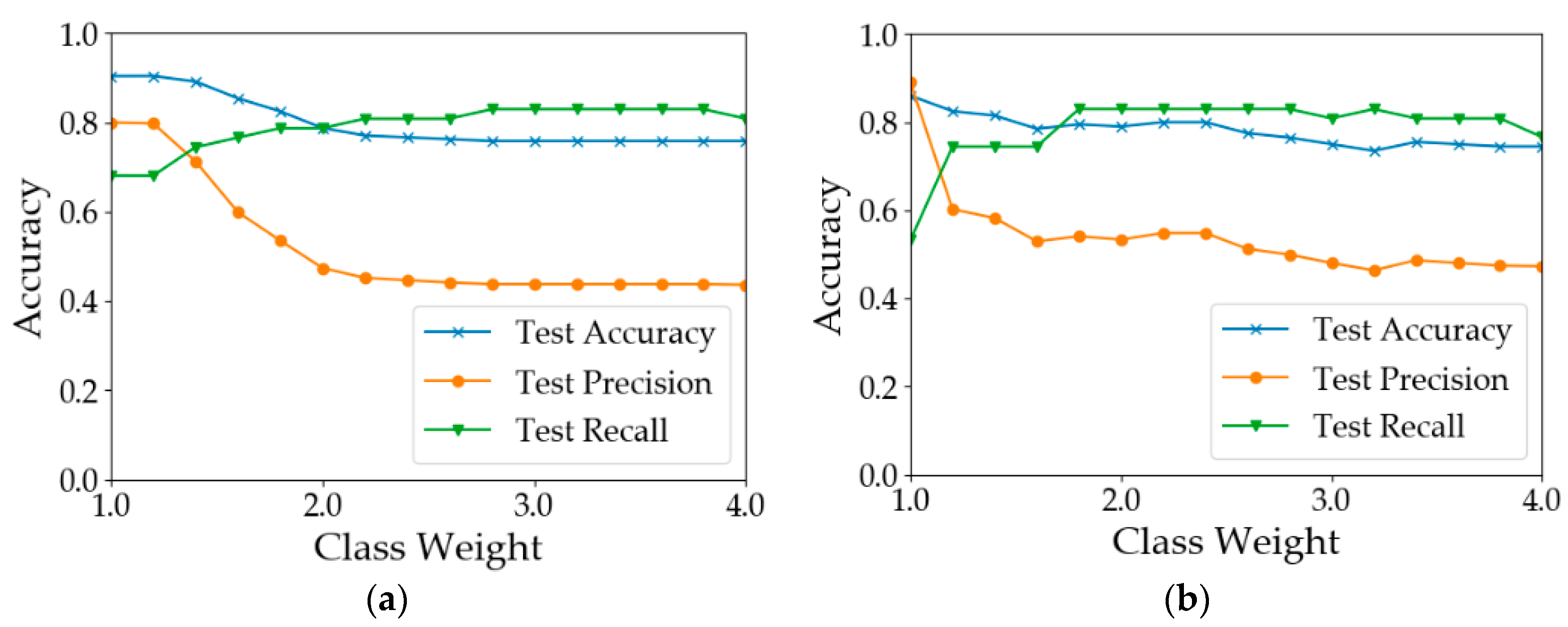
53]. Since the number of samples was limited, the second way was adopted to test model performance by assigning different weights to the minority class samples. The results are shown in
Figure 8. In calculation I (
Figure 8a), when the weight of the ‘disease’ class was increased from 1 to 1.2, the results did not change. When the class weight was between 1.2 and 2.8, with the increase in class weight, the recall of diseased samples increased from 0.681 to 0.830. However, the overall test accuracy and the test precision dropped by 15% and 35%, respectively. In calculation II (
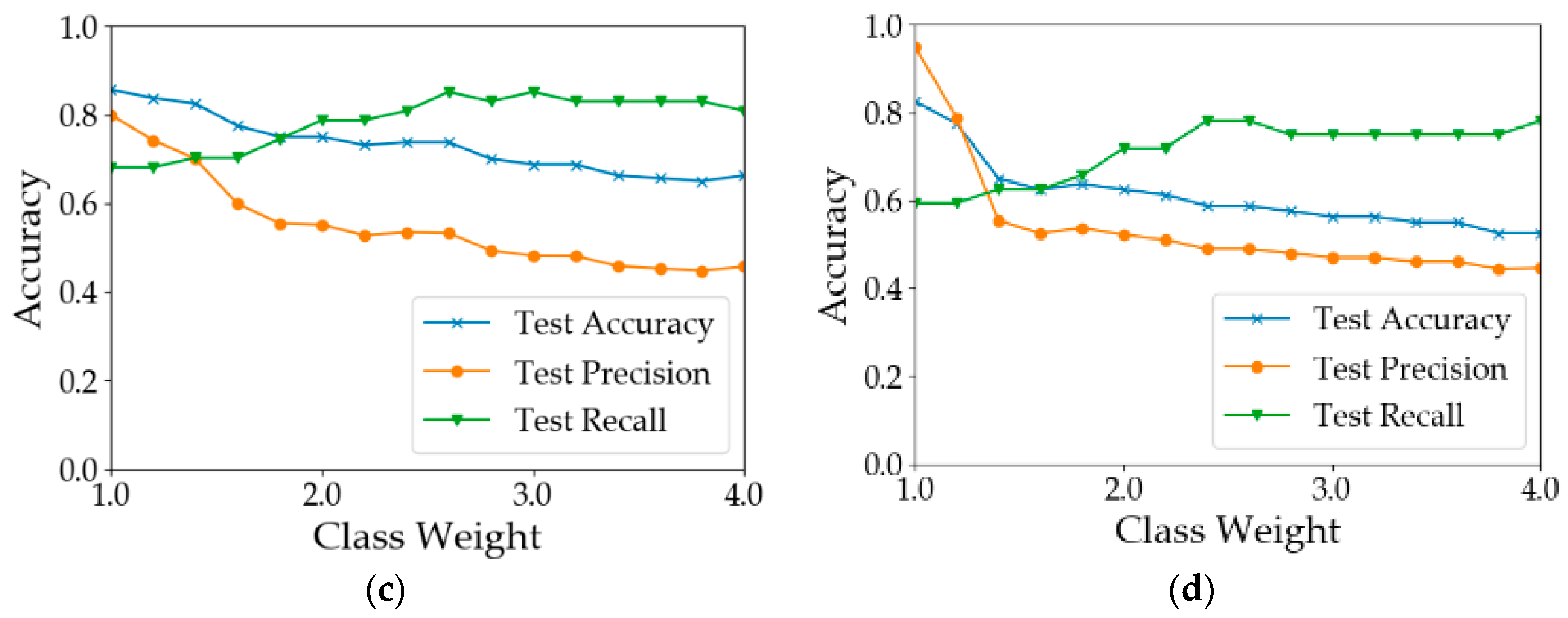
Figure 8b), when the weight was 1.8, the test recall achieved 0.830. After that, the model performance deteriorated with the increase in the class weight. In calculation III (
Figure 8c), the best test recall was achieved when the class weight was increased to 2.6. The overall test accuracy and the test precision dropped by 20% and 34%, respectively. In calculation IV (
Figure 8d), the test recall can be improved to 0.8. In summary, the increase in minority class weight can help improve the classification accuracy of diseased samples. However, the improvement was at the cost of overall accuracy and precision. Therefore, the value of the class weight should be adjusted according to the practical need. If the objective is to detect as many diseased quadrats as possible, a larger value of class weight should be used; otherwise, a smaller value should be used.
3.4. Forecast of the Soybean Sudden Death Syndrome (SDS)
Since the GRU-based method is a time sequence prediction model, it should forecast SDS occurrence in the future. To measure the prediction performance, calculations of four different scenarios have been conducted, as shown in
Table 4. The first method was named as GRU_Current, which is the same as the proposed method in
Section 3.2. The second was named as GRU_Next, which uses time-series imagery to predict SDS at the next time point. The results have been compared with the results in
Table 3. Take calculation A as an example; the target was SDS at time points 3, 4, 5 and 6 in 2016 and time points 5 and 6 in 2017. The sequence length of GRU_Next was two. The sequences were 1-2, 2-3, 3-4 and 4-5 in 2016 and 3-4 and 4-5 in 2017. The sequence length of GRU_Current was three. The sequences were 1-2-3, 2-3-4, 3-4-5 and 4-5-6 in 2016 and 3-4-5 and 4-5-6 in 2017. The two methods have the same target, i.e., SDS at the time points 3, 4, 5 and 6 in 2016 and at time points 5 and 6 in 2017.
The results are shown in
Table 5. In calculations A, B and C, the test accuracy of GRU_Current was 1–3% greater than that of GRU_Next. In terms of test precision and test recall, GRU_Current also outperformed GRU_Next. However, with the increase in the sequence length, the gap between the test accuracy of the two methods becomes smaller. In calculation D, although the train accuracies were slightly different, the test accuracy, recall and precision of the two methods were the same. It indicates that the proposed model can be used to predict the SDS at the next time point when enough historical images are available, which will bring benefits to the prediction of the future development of the plant diseases.
4. Discussion
Remote sensing using satellite imagery can be a potentially powerful tool to detect plant diseases at a quadrat or field level. Our results prove that the stress-triggered changes in the pattern of light emission due to soybean SDS can be detected through high-resolution satellite imagery and the classification accuracy of diseased and healthy quadrats can be further improved by incorporating time-series prediction. Our proposed method has manifested its ability to improve SDS detection accuracy by incorporating time-series information.
A growing interest has been observed recently in the early detection of plant diseases. Researchers have used different remote sensing tools for early detection and monitoring of plant diseases at different spatial levels, such as leaf scale [
54,
55,
56,
57,
58,
59], plant canopy scale [
3,
60], plot-scale based on aerial imagery [
61,
62] and field-wide-scale based on satellite imagery [
29,
63,
64,
65]. Although many studies obtained remotely sensed data at different time points, none of them incorporated time-series information in the analytical models.
Instead of only using individual static imagery, we proposed a model that treats the satellite imagery, captured at different time points, as a time series for the detection of SDS. We compared the SDS prediction results from our proposed GRU-based method with XGBoost and the FCDNN, both non-sequence-based methods. Although the test accuracies of all three methods were above 76%, accuracy improved by up to 7% after incorporating time-series prediction. This substantial improvement in accuracy reveals that the GRU-based method uses the characteristic information of spectral bands, ground-based crop rotation and time series in an optimal way. The main advantage of the GRU-based method goes back to its workability of learning from history data. In the learning process, GRU can determine the influence of images at different time points on the decision-making of the current status through the reset gate and the update gate. Information from past images can help the model to eliminate the effect of some noise, such as weather conditions.
In all calculation scenarios, the GRU-based method outperformed XGBoost and the FCDNN in SDS prediction accuracy. Although XGBoost and the FCDNN are very powerful methods, they do not incorporate time-based information. In our data, we found that reflectance values in the RGB spectrum were lower for healthy quadrats than diseased quadrats, while this was the opposite in the NIR spectrum. Moreover, this pattern became clearer near the end of the cropping season, which indicates that incorporating time-based information for satellite images can add information to the data analysis.
Besides accuracy, the GRU-based method also achieved greater precision (80–95%) for SDS detection in all calculation scenarios, as compared to the XGBoost and FCDNN methods. This means that soybean quadrats predicted either as diseased or healthy were assigned correctly 80% to 95% of the time. However, in terms of recall, the FCDNN performed better than the GRU-based method and XGBoost in three out of four calculation scenarios. This means that the FCDNN predicted diseased soybean quadrats more accurately than the other two methods. However, its test accuracy was lower because this method was not correctly predicting the healthy soybean quadrats. The reason is that FCDNN was more likely to predict a sample as diseased, so the precision was sacrificed.
In the end, we made predictions of SDS at future time points (GRU_Next) based on previous time-based imagery and we compared these results with the predictions made at time points included in the training (GRU_Current). SDS prediction accuracy, precision and recall were greater in GRU_Current models in small sequence scenarios. It is possible that this improved precision is because the models in the GRU_Current scenarios can extract information from the imagery collected at the current time point. On the other hand, in GRU_Next scenarios, we were predicting SDS using the history data only. Moreover, in the last sequence scenario, accuracy, recall and precision of both GRU_Next and GRU_Current models became equal, which indicates that the GRU-based method can predict SDS in soybean quadrats with high accuracy when enough historical images are available.
A recent study [
29] conducted at the same site detected SDS through satellite images with above 75% accuracy using the random forest algorithm. Contrary to our study, they used static images for data analysis and predicted SDS on the 30% test subset from the same satellite images. In comparison, we proposed a method that can predict SDS with high accuracy at future time points, based on time-series satellite imagery.
5. Limitations and Future Work
It should be noted that this proposed plant-disease recognition using a sequence-based model with remote sensing is subject to a few limitations which suggest future research directions.
In the data collection, the number of images in our case study was limited because the PlanetScope satellite can only take pictures of the locations every one or two weeks. More frequent observations of SDS can help the model capture subtle changes along time. Some studies installed a camera system around the canopies or plots so that they can monitor the real-time status of the plants. However, since it requires a high intensity of cameras, the scalability of this method is limited. Another issue of satellite imagery is that the collection frequency of the imagery may not correspond to the development of diseases. As shown in the previous section, SDS development in June and July was slow, while it was much faster at the end of August. So, ideally, it would have been better to collect images more frequently in August. Besides, the locations of the quadrats of 2016 and 2017 were different. Therefore, the time sequences of 2016 and 2017 were constructed separately. In the future, the experimental fields should be evaluated consistently so that longer time sequences can be used to further improve the prediction accuracy.
In terms of data preprocessing, this paper only used the mean values and variance values of the pixels due to the resolution limitations. The importance of different pixels may be different due to disease intensities. One alternative way is to construct a small-scale CNN to obtain features of each image and then feed the extracted features to the GRU. Additionally, multi-band imagery can also be used to improve the accuracy.
In some calculations, the percentage of diseased samples was very low, meaning that the data were not balanced. In this paper, this issue was addressed by assigning weights to the diseased samples in the calculation of loss of function. There are also some other methods to address data imbalance problem. For example, the oversampling method can generate new diseased samples by recombining the pixels of the diseased samples. In the future, we will compare the effectiveness of different methods.
Lastly, in this study, SDS is labeled as diseased (denoted as “1”) and not diseased (denoted as “0”), using 5% as a threshold value which constitutes a classification problem. One concern is the influence of the threshold value on the model performance. For example, in our case, quadrats with 5.1% and 99.1% incidence were categorized as diseased samples, which may influence the prediction precision of the model. Therefore, the classification accuracy of the model will be tested using different threshold values in the future. We can also test other time-series models, e.g., LSTM. These are reserved for future research.
6. Conclusions
The development of sensing techniques has brought significant improvements to plant-disease detection, treatment and management. However, there is a lack of research on detecting SDS using pixel-level satellite imagery at the quadrat level. The major challenge is how to use limited information, i.e., only a few pixels for each quadrat, to improve SDS prediction accuracy. Some traditional methods for the analysis of near-sensing data are based on CNNs, which can efficiently extract the most important features from thousands of RGB values and other information. In contrast, for the analysis of low-pixel-level satellite imagery, additional information is required.
In this paper, a GRU-based model is proposed to predict SDS by incorporating temporality into the satellite imagery. Instead of using individual static imagery, time-series imagery is used to train the model. Different test case scenarios have been created for comparisons between the proposed method and other non-sequence-based methods. The results show that compared to XGBoost and the FCDNN, the GRU-based method can improve overall prediction accuracy by 7%. In addition, the proposed method can potentially be adapted to predict future development of SDS.

 ,
, 


