Article

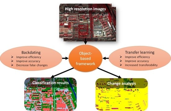
Integrating Backdating and Transfer Learning in an Object-Based Framework for High Resolution Image Classification and Change Analysis

1
State Key Laboratory of Urban and Regional Ecology, Research Center for Eco-Environmental Sciences, Chinese Academy of Sciences, No. 18 Shuangqing Road, Beijing 100085, China
2
College of Resources and Environment, University of Chinese Academy of Sciences, No. 19A Yuquan Road, Beijing 100049, China
3
Beijing Municipal Environmental Monitoring Center, No. 14 Chegongzhuang West Road, Beijing 100048, China
*
Author to whom correspondence should be addressed.
Remote Sens. 2020, 12(24), 4094; https://0-doi-org.brum.beds.ac.uk/10.3390/rs12244094
Submission received: 29 October 2020 / Revised: 6 December 2020 / Accepted: 9 December 2020 / Published: 15 December 2020
(This article belongs to the Special Issue Remote Sensing of Urban Form)

Abstract

:
Classification and change analysis based on high spatial resolution imagery are highly desirable for urban landscapes. However, methods with both high accuracy and efficiency are lacking. Here, we present a novel approach that integrates backdating and transfer learning under an object-based framework. Backdating is used to optimize the target area to be classified, and transfer learning is used to select training samples for classification. We further compare the new approach with that of using backdating or transfer learning alone. We found: (1) The integrated new approach had higher overall accuracy for both classifications (85.33%) and change analysis (88.67%), which were 2.0% and 4.0% higher than that of backdating, and 9.3% and 9.0% higher than that of transfer learning, respectively. (2) Compared to approaches using backdating alone, the use of transfer learning in the new approach allows automatic sample selection for supervised classification, and thereby greatly improves the efficiency of classification, and also reduces the subjectiveness of sample selection. (3) Compared to approaches using transfer learning alone, the use of backdating in the new approach allows the classification focusing on the changed areas, only 16.4% of the entire study area, and therefore greatly improves the efficiency and largely avoid the false change. In addition, the use of a reference map for classification can improve accuracy. This new approach would be particularly useful for large area classification and change analysis.

Graphical Abstract

1. Introduction

Land use/land cover (LULC) change is one of the major drivers of biodiversity loss, air pollution, urban heat island (UHI), water shortage and pollution, and ecosystem degradation from local to regional, and even global scales [1,2]. Remotely sensed images provide an effective way to map and quantify LULC change [3]. While most studies have used medium or coarser resolution data such as Landsat, MODIS, AVHRR, and SPOT-VEGETATION for LULC change analysis [4,5,6], high spatial resolution imagery has been increasingly used to quantify the fine-scale LULC change especially in urban landscapes with a wide availability of such data [7,8].
The backdating/updating and the transfer learning are two promising approaches that use the prior information of an existing land cover map for accurate and efficient classification. The backdating/updating approach conducts the classification in the changing area instead of the whole study area, which brings high efficiency and reduces “false changes” [9]. The transfer learning approach can automatically choose a large number of training samples based on the existing land cover map, which promotes the efficiency of machine learning classification [10].
Recent advances in backdating/updating approaches and transfer learning methods for multi-temporal classifications and/or change analysis show that the proper use of prior knowledge; for example, LULC classes from an existing classification map with high accuracy (typically referred to as “reference map”), can greatly increase the accuracy and efficiency in classification for other time periods, and for change analysis [9,11,12,13]. However, such advances in land cover mapping and change analysis have been largely developed from, and applied to, medium and coarser resolution remote sensing data, but not the increasingly used high spatial resolution images. For example, change analysis using high resolution images is still frequently based on traditional post-classification comparisons [14,15], which is time-consuming and may contain lots of “false changes” due to the propagation of errors from classification maps to the change analysis [16,17]. In the absence of long-term images (such as the Landsat satellite images) and global land cover products (such as the GlobeLand30), few studies have tested whether such advances in classification and change analysis can be applied to high spatial resolution imagery [9,10,18]. In particular, can a combination of such advances significantly improve accuracy and efficiency when using high spatial resolution imagery?
The strength of an updating/backdating approach lies in the application of prior knowledge based on existing LULC classification maps (i.e., reference maps) to classify the areas with changes, and update/backdate the areas with no change [12]. With classification focusing on a small proportion of the study areas with the change, and the application of prior knowledge of existing LULC types, an updating/backdating approach can greatly improve both efficiency and accuracy of multi-temporal classifications and change analysis [9,12,13,19,20]. The generation of the National Land Cover Database (NLCD) in the year 2006 and 2011 provides an excellent example of applying such an approach [12,19]. The product of NLCD in 2006 was updated from NLCD 2001 [12], and NLCD 2011 was updated from NLCD 2006 [19]. In addition, when integrating backdating with object-based classification, the accuracy and efficiency can be further improved because the object-based method can help reduce errors caused by, for example, misregistration between multi-temporal images [9].
Transfer learning is a method that can be used to transfer the labels of existing data to identify new ones and has been widely used for visual recognition, text processing, and emotional classification [21,22,23]. It was introduced to LULC classification in recent years and has been increasingly applied [11,20,24,25]. One of the advantages of the transfer learning method is the automatic selection of a very large number of training samples based on land cover type in “reference map”, which can greatly improve the classification accuracy and efficiency, and reduce the subjectiveness of sample selection [26,27]. Transfer learning methods are usually classified into four categories, which are instance transfer, parameter transfer, feature representation transfer, and relational knowledge transfer [10]. Previous studies usually used a relational knowledge transfer framework for land cover classification [10,11,28]. Specifically, they first applied a change detection-based approach to transfer the labels of land cover types from the source domain to the target domain and then used the labeled pixels/objects as training samples to classify the target image. However, this method has been mostly applied in LULC classification using medium and coarser resolution data, not high spatial resolution data.
Due to the much larger data volume of very high spatial resolution data, in comparison with medium and coarser resolution ones when covering the same area, improving the efficiency is highly desirable. Here, we develop a new approach that integrates backdating and transfer learning under an object-based framework. We test this new approach using high spatial resolution GeoEye-1 and Pleiades images in Beijing, China. We further compare the new approach with that of using backdating or transfer learning alone. We used an object-based framework as it has been proved to be superior to a pixel-based approach, especially when using high spatial resolution data [14,29].

2. Study Area and Data Preprocessing

2.1. Study Area

We chose a study area within the 5th ring road of Beijing, China, a location where many changes in LULC occurred between 2009 and 2015 (Figure 1). The study area contains all kinds of typical LULC types in urban settings, such as greenspace (i.e., vegetated land), water, buildings, and paved surfaces. From 2009 to 2015, both changes in large (e.g., a large patch of greenspace was replaced by buildings) and small size occurred in the study area, making it ideal for testing the proposed approach.

2.2. Data Preprocessing

We used the GeoEye-1 image acquired on 28 June 2009, and Pleiades image on 19 September 2015 for our study (Table 1). These two types of images have a similar spatial and spectral resolution. They both have one panchromatic band and four multispectral bands. The spatial resolution of GeoEye-1 and Pleiades for the panchromatic band is similar, 0.41 m and 0.5 m, respectively, and that for multi-spectral bands is 1.65 m and 2 m, respectively. The GeoEye-1 image was taken in summer, resulting in a higher solar elevation angle than that of the Pleiades (Table 1), so the shaded area of the GeoEye-1 is smaller than that of the Pleiades. It is difficult to identify the land cover in the shadow, and it is not the focus of this study. So, we treat shadows as a type of LULC.
We first conducted a radiometric correction for two images using the FLAASH model embedded in ENVI software. Then, we used a linear regression method for relative radiation normalization. That is, each band of the Pleiades image was linearly normalized to the corresponding band of the GeoEye-1 image. After that, we geometrically registered the GeoEye-1 image to the Pleiades image, and resampled the GeoEye-1 image to match the resolution of Pleiades. We chose 15 tie points and used the second-order polynomial model and the nearest neighborhood resampling approach for spatial rectification. The root mean square error was less than 0.5 pixels. For both images, we resampled the multi-spectral bands to the spatial resolution of the panchromatic band, using the nearest neighborhood resampling approach. For all experiments, we used a quad-core processor with a core frequency of 3.70 GHz, and a RAM of 32 GB to run the program. The operating system is window 10 of 64 bit.
I n e w = I M i n M a x M i n   M a x n e w M i n n e w   +   M i n n e w
For each band of the Pleiades image, I is the original pixel value, I n e w is the normalized pixel value; M a x and M i n are the maximum and minimum pixel value of Pleiades image, respectively, M a x n e w and M i n n e w are the maximum and minimum pixel values of the corresponding band of GeoEye-1, respectively.
We first classified the Pleiades image in 2015 using an object-based supervised classification, which was then used as the reference map in the latter backdating analysis. Specifically, we used the multiresolution segmentation algorithm embedded in the commercial software Trimble eCognition for image segmentation [30]. We first resampled the four multispectral bands to match the resolution of the panchromatic band, and then used all five bands for segmentation. We set the segmentation parameters of scale, color weight, and compactness weight to 30, 0.9, and 0.5, respectively, based on the “trial and error” approach. Then, we randomly chose 200 segmented objects as training samples for each typical type of urban land cover, namely greenspace, shadow, water, building, and pavement. Based on these samples, we used the spectrum and shape features, including five image bands, NDVI (Normalized Difference Vegetation Index), NDWI (Normalized Difference Water Index), and length for supervised classification. We used the support vector machine (SVM) as the classifier to classify segmented objects. We used the radial basis function (RBF) kernel of the SVM. According to a previous study [31], we tested the 10 values of C—10−1, 100, 101, 102, 103, 104, 105, 106, 107, and 108—and 10 values of gamma—10−5, 10−4, 10−3, 10−2, 10−1, 100, 101, 102, 103, and 104. Finally, we set parameters C and gamma for the SVM as 106 and 10−5, respectively. After supervised classification, we did extensive manual editing to refine the classification, and then selected 300 test samples, at least 30 samples in each category for accuracy assessment. We used a stratified random sampling method in Erdas Imagine (version 9.1) to generate testing samples, and then visually interpreted the “true” land cover type based on the Pleiades image. Specifically, we generated 72 samples for greenspace, 77 samples for building, 67 samples for pavement, 30 samples for water, and 54 samples for shadow. The final classification accuracy of the reference map was 92.58%.

3. Methods

We used three methods to classify LULC in 2009, as well as the changes from 2009 to 2015: (1) Method 1: a method of using a backdating approach alone; (2) Method 2: a method of using a transfer learning approach alone; and (3) Method 3: the new approach developed in this study that integrates backdating and transfer learning. All three methods were applied with an object-based procedure, which first segments the image into objects, and then classifies the objects. In addition, all three methods used the same reference map, the land cover map of 2015, for classification and change analysis. However, the way of how to use the reference map (Land cover map of 2015) was different for the three methods (Figure 2). After classification, we combined the land cover map of 2009 and 2015 to map the land cover change.

3.1. Method 1: Classification and Change Analysis using Backdating

3.1.1. Image Segmentation

We first segmented the 2009 GeoEye-1 image into objects. To ensure the boundaries of the segmented objects match the land cover patches in 2015, we used the 2015 LULC map as a thematic layer [14]. We segmented the image using multi-resolution segmentation algorithm that was embedded in the commercial software of eCognitionTM. The multi-resolution segmentation algorithm is a bottom-up region merging approach, which consecutively merges pixels or existing image objects into larger ones, according to the criteria of relative homogeneity which is determined by the input image layers [32]. In this study, we set equal weights for the five original bands when calculating the homogeneity.
For multi-resolution segmentation, the parameter “scale” determines the degree of homogeneity for the segmented objects, and thereby determines the average size of segmented objects. In general, the greater the value of the scale, the larger the size of the objects. In addition, two pairs of parameters: color and shape, and compactness and smoothness, affect the shape of segmented objects. Corresponding to the size of different land cover types, we created two object levels. At level one, the lower level, the scale value was set as 50 to separate the objects of fragmented greenspace, buildings, and shadows. At level two, the scale value was set as 200 to segment the relatively large patches of water and pavement. According to previous studies, we set the weights of color and shape as 0.9 and 0.1, respectively, and that of compactness and smoothness as 0.5 for both levels [33,34]. Consequently, we created 14,943 segments in level 1, with the size ranging from 2 pixels to 11,898 pixels. For level 2, we create 1231 segments, ranging in size from 32 pixels to 56,468 pixels. Finally, we merged the tiny segments by setting the minimum mapping units to 100 pixels.

3.1.2. Backdating

Following the image segmentation, we conducted the object-based classification using the backdating approach [9]. The backdating approach first applied change detection to separate changed (classified as “No change”) and unchanged objects (classified as “Possible change”) based on the GeoEye-1 image in 2009 and the Pleiades image in 2015. Then, it classified the changed objects using rule-based classification and assigned the unchanged objects as the same LULC classes as that of the reference map in 2015 (the land cover map of 2015). All changed and unchanged objects were finally classified into one of the five land cover types: greenspace, building, pavement, water, and shadow (Figure 3).
(1)
Change detection
We applied the change vector analysis (CVA) approach to identify objects with change [12,35,36,37]. The change vector (CV) was calculated for each object based on the two normalized images. For each object, we used the vectors R and S to represent the bands of GeoEye-1 image and Pleiades image, respectively (Equation (1)).
R = r 1 r 2 r n ,   S = s 1 s 2 s n
n is the total number of image bands. Here, n equals five. For each object, r1 represents the mean value of the first band of the GeoEye-1 image, and s1 represents the mean value of the same band of the Pleiades image.
For each object, the change magnitude of CV is calculated as Equation (2):
|| Δ V || = r 1 s 1 2 + r 2 s 2 2 + + r n s n 2 1 / 2
||ΔV|| represents the total spectral differences between image 2009 and 2015 for a given object. In general, the greater the value of the ||ΔV||, the higher the possibility of change in land cover type.
With the CVA algorithm, a specific threshold of change magnitude of CV is set to determine whether change occurs to an object (Equation (3)). As the threshold may vary by land cover types, the use of one single threshold for the whole scene may be inappropriate, generally resulting in over-extraction or under extraction [35]. In this study, we used a multi-threshold method, which identified the threshold values of change based on different land cover types [12]. Specifically, we first classified all objects to class j (greenspace, building, pavement, water, and shadow) according to the land cover map of 2015, and then calculated the change magnitude of CV for all objects ( || Δ V j x || ). Using all the objects in class j, we calculated the mean CVj ( || V ¯ j || ) and the standard deviation of the CVj ( σ j ). For each object in class j, we finally classified it to change or unchanged based on Equation (3).
C V j x = c h a n g e   i f || Δ V j x || || V ¯ j || + a j σ j u n c h a n g e   i f || Δ V j x || < || V ¯ j || + a j σ j
For any land cover type j, || V ¯ j || is the mean of all change vector C V j , σ j is the standard deviation of the C V j , and a j is an adjustable parameter. The large value of a j will lead to less changed objects, vice versa.
To find the optimal threshold, we tested a series of values of a j , from 0.1 to 3. We finally set the value of a j as 1.5, which achieved the highest classification accuracy, to identify all the objects that potentially had change. In other words, all land cover classes used a threshold of the mean plus and minus 1.5 times the standard deviation of the C V j to separate changed and unchanged objects. The threshold value was chosen based on a previous study [38]. We classified the objects as “Possible Change” if the value of C V j is larger than the threshold and classified the rest of objects as “No Change”. To calculate the values of || V ¯ j || and σ j for each land cover class, we used the classification result in the reference map to determine the land cover type for each object [12,19].
(2)
Rule-based classification
We used a rule-based approach for this classification, following the method detailed in previous studies [39]. Figure 4 shows the features and thresholds that were used for classification (Figure 4), all threshold values were determined by the “trial and error” approach. Specifically, we first separated shaded objects from non-shaded objects based on the brightness and NDWI of the object. If the value of brightness (the mean value of five original bands) is smaller than 260 and NDWI was smaller than 0.42, we classified them into the class of shadow. For non-shaded objects, we first separated greenspace (i.e., vegetated land) from non-vegetated land. We classified the objects with the value of NDVI greater than 0.55 as greenspace. For non-greenspace objects, we further separated objects of water from non-water. We classified the objects as water if the value of NDWI was greater than 0.40. Non-water objects were further classified as buildings and pavements. Objects with a brightness greater than 500, or with brightness smaller than 415 but NDVI smaller than 0.43 were classified as buildings, and the rest were then classified as pavement.

3.2. Method 2: Classification and Change Analysis using Transfer Learning

3.2.1. Image Segmentation

The process of image segmentation was the same as that in Method 1.

3.2.2. Transfer Learning

We deem the images over two periods as t1 (2009) and t2 (2015). X1 (GeoEye-1) and X2 (Pleiades) are original images acquired at time t1 and t2, respectively. We have classified the land cover at time t2, labeled P2 (the land cover map of 2015) in advance. The goal of the transfer learning is to produce a land cover map based on image X1 with the transferred knowledge from image X2 and land cover labels of P2.
Following the image segmentation, we conducted the object-based classification using the transfer learning approach [10]. The transfer learning approach first applied change detection to select a training sample set and labeled all samples to land cover types based on the land cover map of 2015. With the training sample set, we conducted a supervised classification for the whole study area (Figure 5). All objects were finally classified into one of the five land cover types: greenspace, building, pavement, water, and shadow.
(1)
Change detection
The algorithm of change detection was the same as that in Method 1. The difference is, we tested a series of values of a j , from 0.1 to 1.5, to find the optimal threshold. We finally set the value of a j as 0.4, which achieved the highest classification accuracy. That is, we used a threshold of the mean plus and minus 0.4 times the standard deviation of the C V j for all land cover classes to select training samples. We classified the objects as “training sample” if the value of C V j is smaller than the threshold. To calculate the values of || V ¯ j || and σ j for each land cover class, we used the classification result in the reference map to determine the land cover type for each object [12,19]. Finally, we transferred 360 samples for building, 395 samples for pavement, 89 samples for shadow, 350 samples for greenspace, and 16 samples for water.
(2)
Supervised classification
We used a supervised classification approach based on the transferred training sample set. We selected NDVI, NDWI, brightness, and the DN value of the five original bands as features for supervised classification (Table 2). For the classifier, we compare the classification performance of the support vector machine and random forest. Because the classification accuracy of the random forest was generally 3–5% higher than that of the support vector machine, we finally chose random forest as the classifier. Specifically, we set the maximum number of resulting decision trees as 50, and set the active variables as 3, which is used to determine the best splits for each tree. The maximum tree number was set empirically, and the value of the active variable was set based on the square root of the total number of features [40].

3.3. Method 3: Classification and Change Analysis Integrating Backdating and Transfer Learning

3.3.1. Image Segmentation

The process of image segmentation was the same as that in Method 1.

3.3.2. Backdating & Transfer Learning

Following the image segmentation, we conducted the object-based classification combining the backdating and transfer learning approach. First, we applied change detection to separate changed and unchanged objects based on the GeoEye-1 image in 2009 and the Pleiades image in 2015. Then, we select a training sample set, and labeled all samples to land cover types based on the land cover map of 2015. For the changed objects, we conducted a supervised classification based on the training sample set and Method 2. For example, the changed and unchanged objects were the same as those for the rest unchanged objects, we assigned the same LULC classes as that of the reference map in 2015 (Figure 6). Here, the methods and parameters of backdating and transfer learning were consistent with Method 1. The training sample set was the same as that in Method 2.
For the purpose of applying this method to other images, we need to reset two important parameters. One is the CV threshold that is used to classify change and unchanged objects, the other one is the threshold of CV that is used to select a training sample set. Those two thresholds are calculated based on the parameter aj, the adjustable parameter in change detection. The optimal value of aj can be determined by a “trial and error” approach. In addition, as an object-based classification, the parameters of segmentation also need to be reset according to the classification target.
(1)
Change detection
The algorithm of change detection was the same as that in Method 1. The difference is, Method 3 not only used it to separate changed and unchanged objects, but also used it to select training samples. Specifically, we set the a j as 1.5 to classify change and unchanged objects and set the a j as 0.4 to select training samples.
(2)
Supervised classification
We used the same training samples, classifier, and parameter setting as that of Method 2 for supervised classification. However, different from Method 2, we only conducted the classification for the objects of changed objects (classified as “Possible change”) instead of all objects in the study area. After classification, we combined the land cover map of 2009 and 2015 to map the land cover change.

3.4. Accuracy Assessment

We conducted accuracy assessment for (1) the change detection layer from 2009 to 2015 which were used in Method 1 and Method 3; (2) the sample selection layer from 2009 to 2015 which were used in Method 2 and Method 3; (3) the classification maps resulted from the three methods; and (4) the three change analysis maps from the three methods. We used a pixel-based stratified random sampling scheme in Erdas Imagine (version 9.1) to select testing samples. For the change detection layer and sample selection layer, we selected a total number of 300 samples, with 150 samples for change, 150 samples for no change. For classification maps and change analysis maps, we selected a total number of 300 samples, with at least 30 samples for each category. We used the GeoEye-1 image in 2009 to verify the classification results and used both images in 2009 and 2015 to verify the results of changes. Error matrices were generated to calculate the overall accuracies, user’s and producer’s accuracy, and the Kappa statistics.

4. Results

4.1. Comparison of the Classification Accuracy

Method 3 had the best classification accuracies among the three methods (Figure 7; Table 3, Table 4, Table 5 and Table 6). The overall accuracy and Kappa statistic of Method 3 were 85.33% and 0.82, respectively, slightly higher than that of Method 1 (83.33% and 0.79), and much higher than that of Method 2 (76.00% and 0.70). While the overall accuracies of Method 3 and Method 1 were similar, Method 3 had better classification results on distinguishing buildings and pavements (Figure 8; Table 3 and Table 5). For example, the user’s accuracy of the building of Method 3 was 8.50% greater than that of Method 1, and the producer’s accuracy of the pavement of Method 3 was 6.67% greater than that of Method 1.
For all the three methods, the user’s and producer’s accuracy for pavement were relatively low, especially for Method 2 (Table 5). There are a large proportion of the objects of pavement were misclassified as buildings (Figure 7; Table 5). In addition, some of the objects of pavement were also misclassified as greenspace. The user’s and producer’s accuracy for the pavement of Method 3 were 76.36% and 70.00%, respectively, which were 1.86% and 6.67% higher than that of Method 1, and 17.54% and 36.67% higher than that of Method 2.

4.2. Comparison of the Change Detection Accuracy

For the change detection of “Possible change” and “No change” that used for backdating of Method 1 and Method 3, the overall accuracy and Kappa coefficients were 87.67% and 0.75, respectively (Table 7). The user’s accuracy and producer’s accuracy of “Possible change” were 91.85% and 82.67%. That indicated 91.85% of the detected changes were correct, and 17.33% of the real changes were missing. After the change detection, we classified 16.49% of the study area as “Possible change” and classified the rest 83.51% area as “No change”.
For training samples that were automatically chosen based on transfer learning used in Method 2 and Method 3, the overall accuracy and Kappa coefficient were 86.33% and 0.73, respectively, which were 1.37% and 0.02 lower than that of change detection (Table 8). Although the overall accuracy was lower, the classification accuracy of “no change” which used as transferred samples for supervised classification was higher than that of change detection. The user’s accuracy of no change was 88.11%, 3.87% higher than that of change detection. That means 88.11% of samples used for supervised classification were correctly selected. In addition, the area of those samples accounts for 70.12% of the entire study area.
The accuracy assessment on the change analysis also showed that Method 3 had greater overall accuracy than Method 1 and Method 2. The overall accuracy of Method 3 was 88.67%, and the Kappa statistic was 0.87. The overall accuracy of Method 3 was 4.00% greater than that of Method 1 and 9.00% greater than that of Method 2 (Table 9, Table 10, Table 11 and Table 12). Overall, Method 3 and Method 1 had similar change analysis results for many of the change classes (Table 10 and Table 12). However, Method 3 greatly improved the producer’s accuracy for the classes “09GS to 15SD” (i.e., greenspace in 2009 convert to shadow in 2015) and “09PA to 15SD” (i.e., the pavement in 2009 convert to shadow in 2015). For both methods, the user’s and producer’s accuracy, for the classes “09BLD to 15SD” (i.e., building in 2009 convert to shadow in 2015) and “09PA to 15SD” (i.e., the pavement in 2009 convert to shadow in 2015), was relatively low.
The change analysis maps showed that Method 2 identified more changes than Method 1 and Method 3, which were in fact not real changes (Figure 9). Method 2 identified 827 objects as changed, accounting for 38.82% of the total area, but Method 1 and Method 3 only identified 356 and 340 objects as changed, accounting for 11.98% and 11.87% of the total area, respectively. Consequently, the producer’s accuracy for “NoChange” with Method 2 was 20.41% lower than that of Method 1 and Method 3, resulting in a much lower overall accuracy of Method 2 (Table 10, Table 11 and Table 12). In addition, Method 2 identified 17 types of land cover change, some of which did not exist in the study area, such as the type of change from pavement to water (Figure 9).
For all three methods, misclassifications were mostly related to changes associated with shaded objects. In particular, the user’s and producer’s accuracy for “09BLD to 15SD” and “09PA to 15SD” were very low. Many of these changes were not real changes but were caused by the classification of shaded buildings and pavements into shadow. A close examination of the map showed that objects classified as the shadow in 2015 were frequently a mixture of buildings and pavements. It’s very difficult to separate shaded buildings from shaded pavements without the aid of ancillary data [39].

5. Discussion

Due to the availability of long-term Landsat images and the global land cover products, most previous studies have explored the performance of the backdating or transfer learning approach based on medium resolution images [9,10]. However, with the increasing availability of high resolution data and the cloud platform, such as Google Earth Engine, those methods have a large potential to be widely applied to high resolution images. Here, we examined whether the backdating and transfer learning approaches are also applicable to high resolution images. Compared with the classification accuracy of the medium resolution images, which are usually higher than 85% [9,10,12,19], backdating (83.3%) and transfer learning (76%) achieved relatively lower accuracy when applied to high resolution images. That is mainly because the urban landscapes are highly fragmented, and some urban land cover types have large spectral variety, such as buildings and pavement. In addition, the backdating approach achieved higher classification accuracy and generated less false change than transfer learning. That indicates that compared with direct land cover classification, delivery of the correct classification results from the reference map tends to achieve higher accuracy and largely reduce the errors caused by spatial misregistration.
The new approach that integrates backdating and transfer learning was superior to Method 1 using backdating alone and Method 2 using transfer learning alone, in terms of both classification accuracy and efficiency. Comparing to the backdating method, the new approach integrates transfer learning, and thereby can automatically select the training samples. By doing this, it not only reduces the subjectiveness in training sample selection, but also minimizes the manual work of sample selection that can be labor-intensive, and thus makes the selection of a large number of training samples feasible and effective [11,20,24]. The use of a large number of training samples is necessary and useful for improving the classification accuracy of certain classes such as buildings that have large within-class spectral variations [41,42]. Comparing to the transfer learning method, the new approach was more accurate and efficient in classification and change analysis. This is because the integration of backdating allows the use of classification from the reference map for the unchanged areas, which account for 83.51% of the study area [17].
In the classification procedure, two parameters need to be properly set, especially when we transfer this approach to other regions or images. One is the parameter a j that controls the change detection, which decided where to conduct the classification. The other is the parameter a j that controls the sample selection, which decided what information will be used for classification. The first parameter decides the trade-offs of Method 3 with respect to Methods 1 and Method 2. In the extreme case that if we set a very large a j in change detection, we will identify no changed objects in our study area and resulting in the same classification results as Method 1. On the contrary, if we set a very small a j in change detection, the whole study area will be classified as change, and lead to the same classification results as Method 2. The proper thresholds will identify the real changes and select the correct training samples, which will finally determine the classification accuracy. In this study, the thresholds of these two parameters were determined by the “trial and error” approach, which required manual intervention. In the future, if we can develop algorithms to automatically choose the optimal thresholds of the two parameters, this new approach will be more efficient and transferrable.
The image misregistration between two images which presented as the boundary inconsistent is a bottleneck for improving the accuracy of in change analysis [43,44]. Regardless of using medium or high resolution imagery, previous studies have shown that compared with pixel-based classification, the object-based framework can greatly reduce the error in change detection caused by spatial misregistration [9,45,46]. In our method, we used the reference map as the thematic layer in the segmentation procedure. Specifically, we used the borders of land cover patches in the reference map to restrict the segmentation of new objects, which resulting in consistent borders, reduced the error caused by spatial misregistration, especially for images from different sensors. In addition, the object-based approach can incorporate the spatial, textural, and neighboring features in classification, which have great potential to increase the classification accuracy [39].
With the substantial improvement in classification and change analysis accuracy and efficiency, the new approach provides an effective means for large area classification and change analysis using high spatial resolution imagery. Compared with medium and coarser resolution image data, high spatial resolution images have a larger data size, greater within-class spectral variations, and are more affected by spatial misregistration [39,47]. Such a new approach is highly desirable for high spatial resolution data. At present, the lack of a high-resolution land cover product, the “reference map” of the new method, has limited the use of this new approach. The long-term monitoring of urban LULC dynamics is commonly based on medium resolution data such as the 30 m Landsat images [48]. In the future, however, with the development of global high-resolution land cover products [49], this approach is expected to realize the long-term and high-frequency monitoring of fine-scale LULC changes in urban areas based on high-resolution images.

6. Conclusions

For the accurate and efficient classification and change analysis of high spatial resolution imagery, we present a novel approach that integrates backdating and transfer learning under an object-based framework. The new approach first uses backdating to identify the target area for classification and then uses transfer learning to automatically select training samples for supervised classification. Compare to the backdating or transfer learning approaches which were usually separately used for classification, the new approach that combines these two approaches can improve the accuracy. The overall accuracy of classifications and change analysis were 85.33% and 88.67%, respectively, which were 2.0% and 4.0% higher than that of backdating, and 9.3% and 9.0% higher than that of transfer learning. In addition, the new method can promote efficiency in sample selection and classification, and largely reduce false change. In the classification procedure, two parameters need to be properly set especially when we transfer this approach to other regions or images. One is the parameter that controls the change detection, which decided where to conduct the classification. The other is the parameter that controls the sample selection, which decided what information will be used for classification. In the future, with the development of global high-resolution land cover products, this approach is expected to realize the high-resolution land cover classification of long-time series in urban areas.

Author Contributions

Conceptualization, Y.Q., W.Z. (Weiqi Zhou) and L.H.; Formal analysis, Y.Q.; Funding acquisition, W.Z. (Weiqi Zhou); Investigation, W.Z. (Wenhui Zhao); Methodology, W.Y., L.H. and W.L.; Resources, W.Y.; Writing—original draft, Y.Q.; Writing—review & editing, W.Z. (Weiqi Zhou). All authors have read and agreed to the published version of the manuscript.

Funding

The supports of the National Key Research and Development Program of China (Grant Nos. 2016YFC0503004), the National Natural Science Foundation of China (Grant Nos. 41601180 and 41771203), and the Bureau of Ecology and Environment of Shenzhen (SZCG2018161498) are gratefully acknowledged. All authors have read and agreed to the published version of the manuscript.

Conflicts of Interest

The authors declare no conflict of interest.

References

  1. Turner, B.L.; Lambin, E.F.; Reenberg, A. The emergence of land change science for global environmental change and sustainability. Proc. Natl. Acad. Sci. USA 2007, 104, 20666–20671. [Google Scholar] [CrossRef] [PubMed] [Green Version]
  2. Grimm, N.B.; Faeth, S.H.; Golubiewski, N.E.; Redman, C.L.; Wu, J.; Bai, X.; Briggs, J.M. Global Change and the Ecology of Cities. Science 2008, 319, 756–760. [Google Scholar] [CrossRef] [PubMed] [Green Version]
  3. Hansen, M.C.; Loveland, T.R. A review of large area monitoring of land cover change using Landsat data. Remote Sens. Environ. 2012, 122, 66–74. [Google Scholar] [CrossRef]
  4. Wickham, J.; Stehman, S.V.; Gass, L.; Dewitz, J.A.; Sorenson, D.G.; Granneman, B.J.; Poss, R.V.; Baer, L.A. Thematic accuracy assessment of the 2011 National Land Cover Database (NLCD). Remote Sens. Environ. 2017, 191, 328–341. [Google Scholar] [CrossRef] [Green Version]
  5. Bontemps, S.; Bogaert, P.; Titeux, N.; Defourny, P. An object-based change detection method accounting for temporal dependences in time series with medium to coarse spatial resolution. Remote Sens. Environ. 2008, 112, 3181–3191. [Google Scholar] [CrossRef]
  6. Eklundh, L.; Johansson, T.; Solberg, S. Mapping insect defoliation in Scots pine with MODIS time-series data. Remote Sens. Environ. 2009, 113, 1566–1573. [Google Scholar] [CrossRef]
  7. Huang, B.; Zhao, B.; Song, Y. Urban land-use mapping using a deep convolutional neural network with high spatial resolution multispectral remote sensing imagery. Remote Sens. Environ. 2018, 214, 73–86. [Google Scholar] [CrossRef]
  8. Zhang, X.; Du, S. Learning selfhood scales for urban land cover mapping with very-high-resolution satellite images. Remote Sens. Environ. 2016, 178, 172–190. [Google Scholar] [CrossRef]
  9. Yu, W.; Zhou, W.; Qian, Y.; Yan, J. A new approach for land cover classification and change analysis: Integrating backdating and an object-based method. Remote Sens. Environ. 2016, 177, 37–47. [Google Scholar] [CrossRef]
  10. Lin, C.; Du, P.; Samat, A.; Li, E.; Wang, X.; Xia, J. Automatic Updating of Land Cover Maps in Rapidly Urbanizing Regions by Relational Knowledge Transferring from GlobeLand30. Remote Sens. Basel 2019, 11, 1397. [Google Scholar] [CrossRef] [Green Version]
  11. Wu, T.; Luo, J.; Xia, L.; Shen, Z.; Hu, X. Prior Knowledge-Based Automatic Object-Oriented Hierarchical Classification for Updating Detailed Land Cover Maps. J. Indian Soc. Remote 2015, 43, 653–669. [Google Scholar] [CrossRef]
  12. Xian, G.; Homer, C.; Fry, J. Updating the 2001 National Land Cover Database land cover classification to 2006 by using Landsat imagery change detection methods. Remote Sens. Environ. 2009, 113, 1133–1147. [Google Scholar] [CrossRef] [Green Version]
  13. Jin, S.M.; Yang, L.M.; Danielson, P.; Homer, C.; Fry, J.; Xian, G. A comprehensive change detection method for updating the National Land Cover Database to circa 2011. Remote Sens. Environ. 2013, 132, 159–175. [Google Scholar] [CrossRef] [Green Version]
  14. Zhou, W.Q.; Troy, A.; Grove, M. Object-based land cover classification and change analysis in the Baltimore metropolitan area using multitemporal high resolution remote sensing data. Sensors 2008, 8, 1613–1636. [Google Scholar] [CrossRef] [Green Version]
  15. Milani, G.; Volpi, M.; Tonolla, D.; Doering, M.; Robinson, C.; Kneubühler, M.; Schaepman, M. Robust quantification of riverine land cover dynamics by high-resolution remote sensing. Remote Sens. Environ. 2018, 217, 491–505. [Google Scholar] [CrossRef]
  16. Stow, D. Reducing the effects of misregistration on pixel-level change detection. Int. J. Remote Sens. 1999, 20, 2477–2483. [Google Scholar] [CrossRef]
  17. Lu, D.; Mausel, P.; Brondizio, E.; Moran, E. Change detection techniques. Int. J. Remote Sens. 2004, 25, 2365–2407. [Google Scholar] [CrossRef]
  18. Wu, T.; Luo, J.; Zhou, Y.n.; Wang, C.; Xi, J.; Fang, J. Geo-Object-Based Land Cover Map Update for High-Spatial-Resolution Remote Sensing Images via Change Detection and Label Transfer. Remote Sens. Basel 2020, 12, 174. [Google Scholar] [CrossRef] [Green Version]
  19. Xian, G.; Homer, C. Updating the 2001 National Land Cover Database Impervious Surface Products to 2006 using Landsat Imagery Change Detection Methods. Remote Sens. Environ. 2010, 114, 1676–1686. [Google Scholar] [CrossRef]
  20. Rasi, R.; Beuchle, R.; Bodart, C.; Vollmar, M.; Seliger, R.; Achard, F. Automatic Updating of an Object-Based Tropical Forest Cover Classification and Change Assessment. IEEE J. Sel. Top. Appl. Earth Obs. Remote Sens. 2013, 6, 66–73. [Google Scholar] [CrossRef]
  21. Do, C.B.; Ng, A.Y. Transfer learning for text classification. Adv. Neural Inf. Process. Syst. 2005, 18, 299–306. [Google Scholar]
  22. Burgess, E.W. The Growth of the City: An Introduction to a Research Project. City 2008, 18, 71–78. [Google Scholar]
  23. Deng, J.; Zhang, Z.; Marchi, E.; Schuller, B. Sparse autoencoder-based feature transfer learning for speech emotion recognition. In Proceedings of the 2013 Humaine Association Conference on Affective Computing and Intelligent Interaction, Geneva, Switzerland, 2–5 September 2013; pp. 511–516. [Google Scholar]
  24. Xia, L.; Luo, J.; Wang, W.; Shen, Z. An Automated Approach for Land Cover Classification Based on a Fuzzy Supervised Learning Framework. J. Indian Soc. Remote 2014, 42, 505–515. [Google Scholar] [CrossRef]
  25. Xue, L.; Zhang, L.; Bo, D.; Zhang, L.; Qian, S. Iterative Reweighting Heterogeneous Transfer Learning Framework for Supervised Remote Sensing Image Classification. IEEE J. Sel. Top. Appl. Earth Obs. Remote Sens. 2017, 10, 2022–2035. [Google Scholar]
  26. Tuia, D.; Persello, C.; Bruzzone, L. Domain Adaptation for the Classification of Remote Sensing Data: An Overview of Recent Advances. IEEE Geosci. Remote Sens. Mag. 2016, 4, 41–57. [Google Scholar] [CrossRef]
  27. Pan, S.J.; Yang, Q. A Survey on Transfer Learning. IEEE Trans. Knowl. Data Eng. 2010, 22, 1345–1359. [Google Scholar] [CrossRef]
  28. Demir, B.; Bovolo, F.; Bruzzone, L. Updating Land-Cover Maps by Classification of Image Time Series: A Novel Change-Detection-Driven Transfer Learning Approach. IEEE Trans. Geosci. Remote 2013, 51, 300–312. [Google Scholar] [CrossRef]
  29. Myint, S.W.; Gober, P.; Brazel, A.; Grossman-Clarke, S.; Weng, Q.H. Per-pixel vs. object-based classification of urban land cover extraction using high spatial resolution imagery. Remote Sens. Environ. 2011, 115, 1145–1161. [Google Scholar] [CrossRef]
  30. Trimble, T. eCognition Developer 8.7 Reference Book. Trimble Ger. GmbH Munich Ger. 2011, 1, 319–328. [Google Scholar]
  31. Qian, Y.; Zhou, W.; Yan, J.; Li, W.; Han, L. Comparing machine learning classifiers for object-based land cover classification using very high resolution imagery. Remote Sens. Basel 2015, 7, 153–168. [Google Scholar] [CrossRef]
  32. Baatz, M.; Schäpe, A. Multiresolution segmentation: An optimizating approach for high quality multi-scale image segmentation. In Proceedings of Beiträge zum AGIT-Symposium; Wichmann Verlag: Salzburg, Austria, 2000; pp. 12–23. [Google Scholar]
  33. Mathieu, R.; Aryal, J.; Chong, A.K. Object-based classification of ikonos imagery for mapping large-scale vegetation communities in urban areas. Sensors 2007, 7, 2860–2880. [Google Scholar] [CrossRef] [PubMed] [Green Version]
  34. Pu, R.L.; Landry, S.; Yu, Q. Object-based urban detailed land cover classification with high spatial resolution IKONOS imagery. Int. J. Remote Sens. 2011, 32, 3285–3308. [Google Scholar] [CrossRef] [Green Version]
  35. Chen, J.; Gong, P.; He, C.Y.; Pu, R.L.; Shi, P.J. Land-use/land-cover change detection using improved change-vector analysis. Photogramm. Eng. Remote Sens. 2003, 69, 369–379. [Google Scholar] [CrossRef] [Green Version]
  36. Johnson, R.D.; Kasischke, E.S. Change vector analysis: A technique for the multispectral monitoring of land cover and condition. Int. J. Remote Sens. 1998, 19, 411–426. [Google Scholar] [CrossRef]
  37. Nackaerts, K.; Vaesen, K.; Muys, B.; Coppin, P. Comparative performance of a modified change vector analysis in forest change detection. Int. J. Remote Sens. 2005, 26, 839–852. [Google Scholar] [CrossRef]
  38. Morisette, J.T.; Khorram, S. Accuracy assessment curves for satellite-based change detection. Photogramm Eng. Remote Sens. 2000, 66, 875–880. [Google Scholar]
  39. Zhou, W.; Huang, G.; Troy, A.; Cadenasso, M. Object-based land cover classification of shaded areas in high spatial resolution imagery of urban areas: A comparison study. Remote Sens. Environ. 2009, 113, 1769–1777. [Google Scholar] [CrossRef]
  40. Breiman, L. Random forests. Mach. Learn. 2001, 45, 5–32. [Google Scholar] [CrossRef] [Green Version]
  41. Dannenberg, M.; Hakkenberg, C.; Song, C. Consistent Classification of Landsat Time Series with an Improved Automatic Adaptive Signature Generalization Algorithm. Remote Sens. Basel 2016, 8, 691. [Google Scholar] [CrossRef] [Green Version]
  42. Gray, J.; Song, C. Consistent classification of image time series with automatic adaptive signature generalization. Remote Sens. Environ. 2013, 134, 333–341. [Google Scholar] [CrossRef]
  43. Blaschke, T. Towards a framework for change detection based on image objects. Göttinger Geogr. Abh. 2005, 113, 1–9. [Google Scholar]
  44. Xiaolong, D.; Khorram, S. The effects of image misregistration on the accuracy of remotely sensed change detection. IEEE Trans. Geosci. Remote 1998, 36, 1566–1577. [Google Scholar] [CrossRef] [Green Version]
  45. Chen, G.; Zhao, K.; Powers, R. Assessment of the image misregistration effects on object-based change detection. ISPRS J. Photogramm. 2014, 87, 19–27. [Google Scholar] [CrossRef]
  46. Liu, D.; Xia, F. Assessing object-based classification: Advantages and limitations. Remote Sens. Lett. 2010, 1, 187–194. [Google Scholar] [CrossRef]
  47. Benediktsson, J.A.; Chanussot, J.; Moon, W.M. Very high-resolution remote sensing: Challenges and opportunities [point of view]. Proc. IEEE 2012, 100, 1907–1910. [Google Scholar] [CrossRef]
  48. Li, X.; Zhou, Y.; Zhu, Z.; Liang, L.; Yu, B.; Cao, W. Mapping annual urban dynamics (1985–2015) using time series of Landsat data. Remote Sens. Environ. 2018, 216, 674–683. [Google Scholar] [CrossRef]
  49. Dong, R.; Li, C.; Fu, H.; Wang, J.; Gong, P. Improving 3-m Resolution Land Cover Mapping through Efficient Learning from an Imperfect 10-m Resolution Map. Remote Sens. Basel 2020, 12, 1418. [Google Scholar] [CrossRef]
Figure 1. Study area and datasets used in this study. Pane (A): a site example of GeoEye-1 image with False-color acquired on 28 June 2009; panel (B): a site example of Pleiades image with False-color acquired on 19 September 2015; panel (C): a LULC map in 2015 (the reference map). False-color composite: near-infrared, red, green band as RGB.
Remotesensing 12 04094 g001
Figure 2. Flowchart of classification and change analysis. Method 1: backdating; Method 2: transfer learning; Method 3: integration of backdating and transfer learning.
Remotesensing 12 04094 g002
Figure 3. Flowchart of land cover classification using backdating. The key steps were highlighted in grey.
Remotesensing 12 04094 g003
Figure 4. The rule-based classification procedure in Method 1, showing the classification tree and features and thresholds used for classification.
Remotesensing 12 04094 g004
Figure 5. Flowchart of land cover classification using transfer learning.
Remotesensing 12 04094 g005
Figure 6. Flowchart of land cover classification integrating of backdating and transfer learning.
Remotesensing 12 04094 g006
Figure 7. The classification results of the three methods.
Remotesensing 12 04094 g007
Figure 8. The zoom-in of classification results of the three methods. We highlighted the classification results in 2009 in gray.
Remotesensing 12 04094 g008
Figure 9. The change analysis results from three methods. The false types of change that did not occur were marked in gray.
Remotesensing 12 04094 g009
Table 1. The information about high resolution images.
GeoEye-1Pleiades
Acquisition Data/Time2009-06-28 03:04 GMT2015-09-19 03:06 GMT
Solar azimuth132.0320 degrees155.5987 degrees
Solar elevation67.3074 degrees49.3733 degrees
Table 2. Object features used for supervised classification.
Object FeaturesDescription
Mean value of blueMean value of the blue band of an image object
Mean value of greenMean value of the green band of an image object
Mean value of redMean value of the red band of an image object
Mean value of near-infraredMean value of the near-infrared band of an image object
Mean value of panchromaticMean value of the panchromatic band of an image object
BrightnessMean value of the 5 original bands
NDVI(near infrared − red)/(near infrared + red)
NDWI(green − near infrared)/(green + near infrared)
Table 3. The classification accuracies in Method 1–3. Bold values refer to the highest accuracies.
Method 1Method 2Method 3
Overall Acc. (%)83.337685.33
Kappa Coefficient0.790.700.82
Producer’s Acc. (%)Greenspace90.4893.6592.06
Water76.7980.3680.36
Building95.0875.4193.44
Pavement63.3333.3370.00
Shadow90.0096.6790.00
User’s Acc. (%)Greenspace77.0395.1676.32
Water100.0093.7597.83
Building75.3259.7483.82
Pavement74.5058.8276.36
Shadow98.1873.4298.18
Table 4. The classification accuracies in Method 1.
Reference Data
ClassesGreenspaceWaterBuildingPavementShadowSum
Greenspace575010274
Water04300043
Building125812477
Pavement55338051
Shadow01005455
Sum6356616060
Producer’s Acc. (%)90.4876.7995.0863.3390
User’s Acc. (%)77.0310075.3274.598.18
Overall Acc. (%)83.33
Kappa Coefficient0.79
Table 5. The classification accuracies in Method 2.
Reference Data
ClassesGreenspaceWaterBuildingPavementShadowSum
Greenspace59111062
Water04502148
Building004631077
Pavement40920134
Shadow010565879
Sum6356616060
Producer’s Acc. (%)93.6580.3675.433.3396.67
User’s Acc. (%)95.1693.7559.7458.8273.42
Overall Acc. (%)76
Kappa Coefficient0.7
Table 6. The classification accuracies in Method 3.
Reference Data
ClassesGreenspaceWaterBuildingPavementShadowSum
Greenspace585110276
Water04500146
Building00578368
Pavement55342055
Shadow01005455
Sum6356616060
Producer’s Acc. (%)92.0680.3693.447090
User’s Acc. (%)76.3297.8383.8276.3698.18
Overall Acc. (%)85.33
Kappa Coefficient0.82
Table 7. The accuracies of change detection in Method 1 and Method 3.
Reference Data
ClassesPossible ChangeNo ChangeSum
Possible change12411135
No change26139165
Sum150150
Producer’s Acc. (%)82.6792.67
User’s Acc. (%)91.8584.24
Overall Acc. (%)87.67
Kappa Coefficient0.75
Table 8. The accuracies of transfer learning for sample selection used in Method 2 and Method 3.
Reference Data
Classified DataPossible ChangeNo ChangeSum
Possible Change13324157
No change17126143
Sum150150
Producer’s Acc. (%)88.6784.00
User’s Acc. (%)84.7188.11
Overall Acc. (%)86.30
Kappa Coefficient0.73
Table 9. The classification accuracies of changes in Method 1–3. Bold values refer to the highest accuracies.
Method 1Method 2Method 3
Overall Acc. (%)84.6779.6788.67
Kappa Coefficient0.830.770.87
Producer’s Acc. (%)NoChange91.8471.4391.84
09GS to 15SD66.6781.2593.75
09GS to 15BLD10096.6796.67
09GS to 15PA10086.6796.67
09BLD to 15SD10063.3363.33
09PA to 15BLD10096.67100
09PA to 15GS10085.3100
09PA to 15SD46.9467.3571.43
User’s Acc. (%)NoChange100100100
09GS to 15SD100100100
09GS to 15BLD10090.6396.67
09GS to 15PA10092.86100
09BLD to 15SD46.1557.5857.58
09PA to 15BLD96.7787.8893.75
09PA to 15GS10085.394.44
09PA to 15SD82.146671.43
Table 10. The classification accuracies of changes in Method 1.
Method 1Reference Data
ClassesNo Change09GS to 15SD09GS to 15BLD09GS to 15PA09BLD to 15SD09PA to 15BLD09PA to 15GS09PA to 15SDSum
No change43000000043
09GS to 15SD03200000032
09GS to 15BLD20300000032
09GS to 15PA00030000030
09BLD to 15SD090030002665
09PA to 15BLD10000300031
09PA to 15GS10000034035
09PA to 15SD05000002227
False Change320000005
Sum5048303030303448
Producer’s Acc. (%)91.8466.67100.00100.00100.00100.00100.0046.94
User’s Acc. (%)100.00100.00100.00100.0046.1596.77100.0082.14
Overall Acc. (%)84.67
Kappa Coefficient0.83
Note: 09SD: shadow in 2009; 09GS: greenspace in 2009; 09BLD: building in 2009; 09PA: pavement in 2009; 15SD: shadow in 2015; 15GS: greenspace in 2015; 15BLD: building in 2015; 15PA: pavement in 2015. False change: the false types of change that did not occur.
Table 11. The classification accuracies of changes in Method 2.
Method 2Reference Data
ClassesNo Change09GS to 15SD09GS to 15BLD09GS to 15PA09BLD to 15SD09PA to 15BLD09PA to 15GS09PA to 15SDSum
No change33000000033
09GS to 15SD03900000039
09GS to 15BLD01292000032
09GS to 15PA11026000028
09BLD to 15SD00003300033
09PA to 15BLD50100290035
09PA to 15GS31000029235
09PA to 15SD060011003249
False Change8002015016
Sum5048303044303434
Producer’s Acc. (%)71.4381.2596.6786.6763.3396.6785.3067.35
User’s Acc. (%)100.00100.0090.6392.8657.5887.8885.3066.00
Overall Acc. (%)79.67
Kappa Coefficient0.77
Note: 09SD: shadow in 2009; 09GS: greenspace in 2009; 09BLD: building in 2009; 09PA: pavement in 2009; 15SD: shadow in 2015; 15GS: greenspace in 2015; 15BLD: building in 2015; 15PA: pavement in 2015. False change: the false types of change that did not occur.
Table 12. The classification accuracies of changes in Method 3.
Reference Data
ClassesNo Change09GS to 15SD09GS to 15BLD09GS to 15PA09BLD to 15SD09PA to 15BLD09PA to 15GS09PA to 15SDSum
NoChange45000000045
09GS to 15SD04500000045
09GS to 15BLD00291000030
09GS to 15PA00029000029
09BLD to 15SD00003300033
09PA to 15BLD10100300032
09PA to 15GS30000034037
09PA to 15SD030011003448
False Change100000001
Sum5048303044303434
Producer’s Acc. (%)91.8493.7596.6796.6763.33100.00100.0071.43
User’s Acc. (%)100.00100.0096.67100.0057.5893.7594.4471.43
Overall Acc. (%)88.67
Kappa Coefficient0.87
Note: 09SD: shadow in 2009; 09GS: greenspace in 2009; 09BLD: building in 2009; 09PA: pavement in 2009; 15SD: shadow in 2015; 15GS: greenspace in 2015; 15BLD: building in 2015; 15PA: pavement in 2015. False change: the false types of change that did not occur.
Publisher’s Note: MDPI stays neutral with regard to jurisdictional claims in published maps and institutional affiliations.

