An Aircraft Wetland Inundation Experiment Using GNSS Reflectometry


1
Engineering and Science Division, Jet Propulsion Laboratory, California Institute of Technology, Pasadena, CA 91109, USA
2
COSMIC Group, University Corporation for Atmospheric Research, P.O. Box 3000, Boulder, CO 80307-3000, USA
*
Author to whom correspondence should be addressed.
Remote Sens. 2020, 12(3), 512; https://0-doi-org.brum.beds.ac.uk/10.3390/rs12030512
Submission received: 6 December 2019
/
Revised: 24 January 2020
/
Accepted: 24 January 2020
/
Published: 5 February 2020
(This article belongs to the Special Issue Applications of GNSS Reflectometry for Earth Observation)
Abstract
:In early May of 2017, a flight campaign was conducted over Caddo Lake, Texas, to test the ability of Global Navigation Satellite System-Reflectometry (GNSS-R) to detect water underlying vegetation canopies. This paper presents data from that campaign and compares them to Sentinel-1 data collected during the same week. The low-altitude measurement allows for a more detailed assessment of the forward-scattering GNSS-R technique, and at a much higher spatial resolution, than is possible using currently available space-based GNSS-R data. Assumptions about the scattering model are verified, as is the assumption that the surface spot size is approximately the Fresnel zone. The results of this experiment indicate GNSS signals reflected from inundated short, thick vegetation, such as the giant Salvinia observed here, results in only a 2.15 dB loss compared to an open water reflection. GNSS reflections off inundated cypress forests show a 9.4 dB loss, but still 4.25 dB above that observed over dry regions. Sentinel-1 data show a 6-dB loss over the inundated giant Salvinia, relative to open water, and are insensitive to standing water beneath the cypress forests, as there is no difference between the signal over inundated cypress forests and that over dry land. These results indicate that, at aircraft altitudes, forward-scattered GNSS signals are able to map inundated regions even in the presence of dense overlying vegetation, whether that vegetation consists of short plants or tall trees.
1. Introduction
Mapping wetland extent and quantifying how the extent changes over time is an important task for both scientific and societal applications. Wetlands are the largest natural emitter of atmospheric methane, a potent greenhouse gas, yet with the widest uncertainty range [1], and feedbacks between wetlands and the global carbon cycle are still poorly understood [1,2,3,4]. Understanding wetland dynamics is important for predicting the transmission of mosquito-borne diseases like malaria [5], and quantifying the rapid rate of wetland collapse is also important, as they provide economic and ecologic benefits to surrounding communities [6].
Current techniques used to map wetlands are not able to fully capture the sometimes-rapid changes in wetland extent, high spatial variability in inundated or saturated areas, or successfully map water beneath dense vegetation canopies. For example, in situ observations of wetlands are often sparse and seldom made, as many wetlands are located in areas too remote to map regularly. Satellite remote sensing has been widely used to map wetlands and seasonal changes in wetland extent. Optical techniques (e.g., [7]) are unable to map water underneath vegetation or see the land surface through cloud cover, both of which decrease the temporal frequency of observations and underestimate the total extent of inundated areas. Microwave instruments onboard satellites, either monostatic synthetic aperture radars (SARs) or radiometers, are able to see through clouds and, depending on the wavelength, some amount of vegetation cover. Currently available products deriving inundation extent from microwave instruments have primarily used data from radiometers, with an extremely coarse (>25 km) spatial footprint [8,9]. Data from SARs have also been used extensively to quantify seasonal changes in inundation extent in wetland complexes (e.g., [10]), though the only publicly available data are from C-band, which cannot penetrate dense vegetation cover, and the long temporal repeat cycles of a single SAR instrument inhibits their ability to capture short term changes in inundation dynamics.
A new observational technique, Global Navigation Satellite System Reflectometry (GNSS-R), has shown promise to map wetland inundation, even in the presence of dense, overlying vegetation. In [11], significantly higher power was observed in reflections over inundated rice fields compared to dry land. These results motivated a dedicated flight campaign to observe GNSS reflections over a variety of wetland sites and vegetation types, with a focus on Caddo Lake, located on the Texas-Louisiana border. Caddo Lake was chosen because it is one of the most heavily vegetated bodies of water in North America—large portions of the lake are densely covered with tall cypress forests. The cypress forests stand up to 50 m tall, and the trees are sometimes surrounded by cypress knees, which are small knobby structures that support the cypress trees’ stability. Cypress knees stand 20–30 cm above the water surface and prevent the passage of even the smallest watercraft through the forests. In addition to the cypress trees, a distinctive feature of Caddo Lake is the presence of an invasive floating weed, giant Salvinia (Salvinia molesta). These floating mats can completely obscure the open water and move with the lake currents—infestations can appear and disappear within a matter of weeks.
In addition to [11], there have been additional investigations into the potential of GNSS-R to map wetlands using CYGNSS (Cyclone Global Navigation Satellite System; e.g., [12,13,14]), a constellation of space-based GNSS-R instruments. However, these studies have been limited by the spatial footprint of the CYGNSS measurement (7 km × 1 km), which is artificially large due to its optimization for ocean surface remote sensing. With a footprint of this size, it is nearly guaranteed that there will be multiple landcover types contributing to surface scattering within each footprint. The aircraft GNSS-R experiment presented here allows a more detailed assessment of GNSS-R’s forward-scattering geometry, and at a much higher spatial resolution. In particular, it allows for the quantification of the attenuation of the GNSS-R signal through specific canopy types, with less uncertainty introduced by mixed pixels. Other GNSS-R aircraft flight experiments have been done in the past (e.g., [15,16]), though these experiments were for the purpose of understanding the sensitivity of GNSS-R to soil moisture and typical agricultural crops and not for the purpose of sensing standing water under trees.
This study will present GNSS-R data from the aircraft experiment over Caddo Lake and quantify the attenuation of the signal through the vegetation that typifies the Caddo Lake area to better understand the potential of GNSS-R to map inundation underneath different types of vegetation canopies. In order to put the results in the context of other remote sensing techniques, we will compare the results to those from Sentinel-1, a C-band SAR instrument that is routinely used to map inundation dynamics in wetland areas. Although it is well known that, in theory, L-band data should be able to penetrate further into a dense vegetation canopy and therefore be more sensitive to water underneath vegetation, there have been no quantitative assessments of the increased ability of GNSS-R to sense inundation relative to Sentinel-1 when the data collected by the two instruments are on a similar spatial scale. The comparison with Sentinel-1 will quantitatively show the increase in sensitivity of GNSS-R to inundation for specific wetland types relative to the more well-known and trusted Sentinel-1 data.
2. Experimental Campaign
This section describes the GNSS-R instrument, flight setup, and antenna calibration experiment.
2.1. Aircraft Flights
Keystone Ariel Survey, Inc. (Keystone) provided the aircraft, a Cessna 310, for this experiment, as shown in Figure 1a. Keystone also provided a pilot, while we ran the equipment, verified it was working in flight, and oversaw the data collection and flight plan. Most flight data were collected while flying at between 2.4 km (8000’) and 3 km (10,000’) altitude. The flight over the Caddo Lake region took place on 2 May 2017, and consisted of a flight in the morning, when large North/South (N/S) and East/West grids centered on Caddo Lake were performed. During the afternoon flight, another N/S grid at a lower altitude was performed, followed by multiple passes over the Northwest region of Caddo Lake, which has especially dense vegetation over the water. We separately toured this Northwest region that morning by boat to collect in situ data on inundation and tree density.
2.2. Flight Equipment
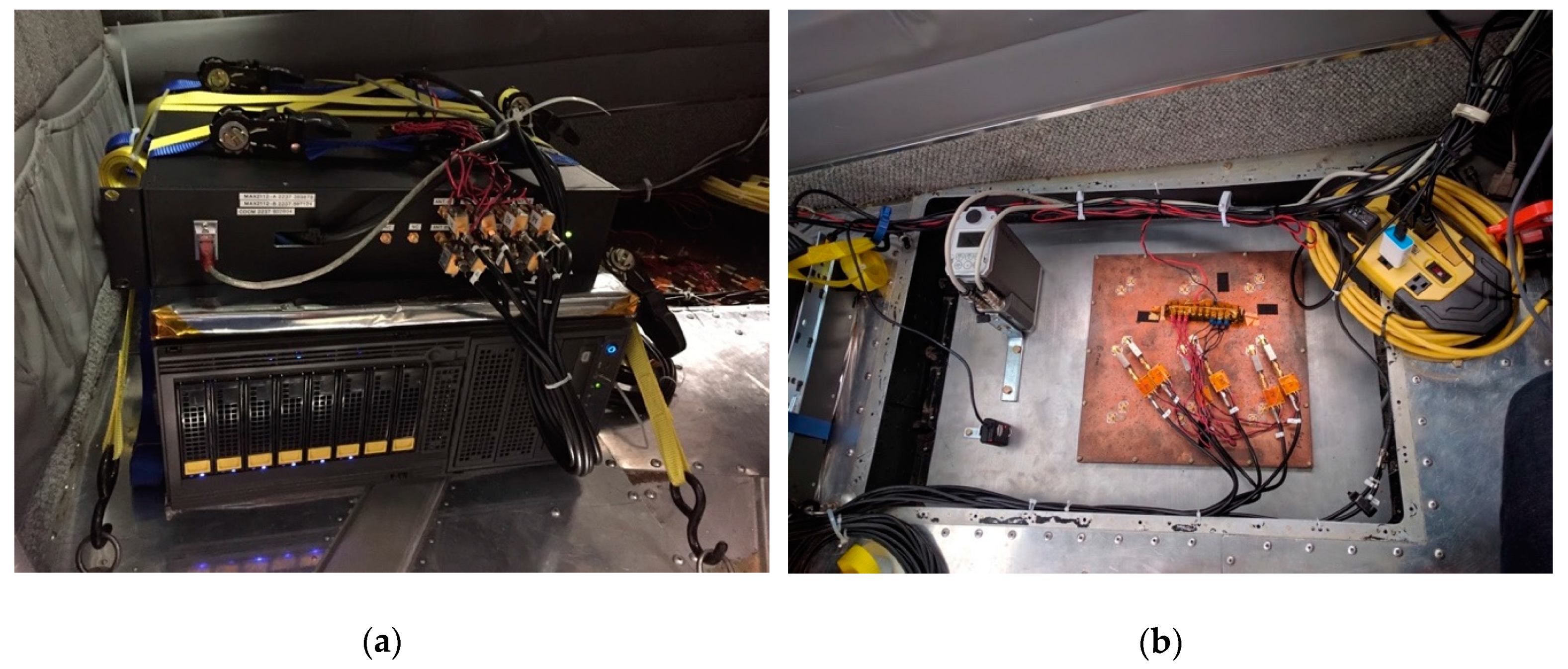
The Cessna 310 had been modified to have a large hole on the underside of the aircraft, which was typically used by Keystone for their commercial optical surveys. For our experiments, Keystone removed their optical camera, and the hole covered with an aluminum plate hosting a 9-element, down-looking, patch array antenna, mounted flush with the airframe. Each patch antenna element provided dual polarization, horizontal and vertical (H/V), at both GPS L1 and L2 frequencies. We flew a custom open-loop recorder, capable of recording up to 40 MHz 1-bit samples from 32 channels. Our front-end electronics had eight antenna inputs, each electronically tunable to two simultaneous local-oscillator (LO) frequencies, resulting in 16 complex (I/Q) sampled data streams, or 32 single-bit sampled streams, matching our recorder’s capability. Figure 2 shows our instruments and down-looking antenna. The recorder was monitored in real time during the flight using a laptop computer.
The Cessna had installed an up-looking commercial aircraft GPS antenna, mounted on top of the aircraft, along with a commercial Novatel GPS receiver, for its navigation system. We split the signal going from this antenna to the Novatel to gain access to the direct signal. For our experiments, we used seven of the eight antenna inputs, recording the H and V outputs from three of the down-looking patch antennas, along with the direct signal from the aircraft’s up-look antenna, all at both the GPS L1 and L2 frequencies. For the Caddo Lake experiment, we combined the H and V outputs from a 4th patch element to form a Left-Hand Circularly Polarized (LCP) signal, and recorded the GPS L1 and L5 frequencies from that patch element.
Most of our data were collected with a sampling rate of 20 MHz, however, some 40 MHz sampled data were collected during the afternoon flight. Our sampled data was stored onto a disk array of SSD hard drives having a total capacity of 8 TB. This allowed about 15 h of continuous recording using a 20 MHz sampling rate.
In addition to the patch antenna and corresponding recording system, we flew a downward-pointing optical camera fastened to the aluminum antenna mount over a small viewing hole, which took high quality optical images every 2 s. Finally, for aircraft positioning, we used the output from the Novatel receiver Keystone had installed on their plane.
2.3. Antenna Calibration
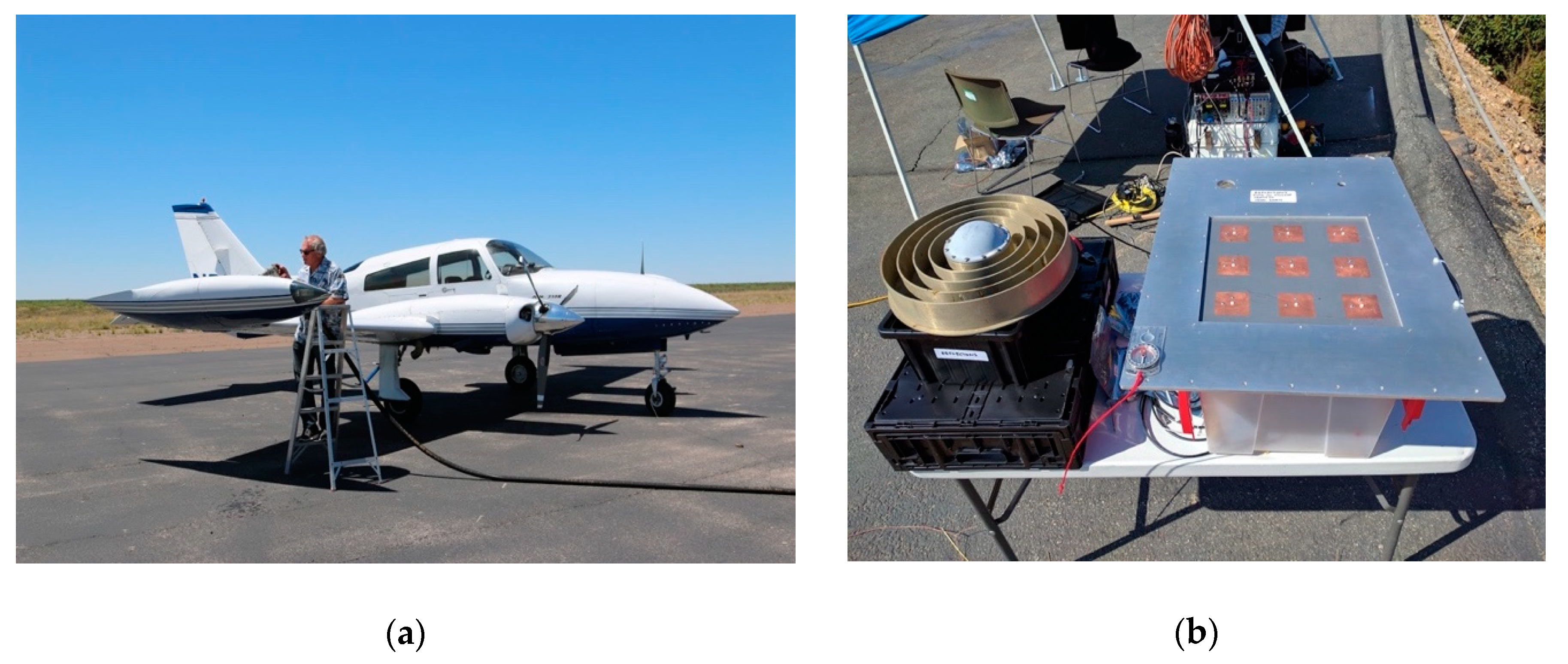
After a preliminary examination of the data, it was clear that the theoretical antenna gain pattern being used for the downward-looking patch elements resulted in geometrically correlated inconsistencies in the resulting surface scattering coefficient. It was assumed that a measurement of the antenna gain pattern would help remove these effects. With limited funding, we chose to perform a simple antenna calibration experiment, differencing the measured gains between our flight antenna and a well-measured geodetic antenna while observing GPS signals as their positions in the sky moved over several hours.
On 21 August 2018, both our 9-element patch array antenna and a well-measured geodetic choke-ring antenna were located near Jet Propulsion Laboratory’s (JPL’s) antenna range at a site with clear open sky views and few nearby objects to minimize multipath, as shown in Figure 1b. The antennas were placed up-looking, with the patch antenna configured as it was during flight, mounted on its aluminum plate with the same low-noise amplifiers (LNAs) on each antenna input. Data were collected as in the aircraft experiment, but with the aircraft’s up-looking geodetic antenna replaced with our choke ring antenna. Although these antennas were placed near each other, we did not observe any mutual coupling. We collected over 7 h of data in two continuous sessions, rotating the patch antenna 180 degrees in the second session for better azimuthal coverage. Since both antennas observed the same GPS transmitters and were located the same distance from them, the ratio of observed power between the antennas would be equal to the ratio of the antenna gains in that direction. By observing over several hours while the geometry of the transmitters changed, and knowing the gain pattern of the geodetic antenna, the patch antenna’s relative gain pattern over much of its beam pattern could be measured. The peak measured gain of the geodetic antenna was 6.8 dBIc while each linear polarization of a single patch was measured to have a peak gain of 5.4 dBIc.
3. Data Processing
The primary GNSS-R observable is a delay-Doppler map (DDM), two-dimensional cross-correlations between the received reflected GNSS signal, and a replica of the transmitted signal. Our DDMs were processed in a similar way as in previous studies [11,17,18].
3.1. Software Receiver and Geometric Modeling
The 20 MHz and 40 MHz raw samples recorded from the aircraft’s usual GPS antenna on top of the plane were processed through a software GPS receiver. All of the GPS signals in view were detected and tracked with delay and phase locked loops. The models used to track these signals were recorded, along with the correlation results. The main processing pass for GNSS-R used these models derived from the direct signals to correlate with data from the down-looking patch arrays.
All correlations were performed coherently each 20 msec. The correlations were performed while offsetting the data relative to the models by between −50 and +500 samples, or lags. The 550 correlations were computed for five Doppler values ranging from −2 to +2 times 39 Hz, using Fast Fourier Transforms (FFTs) and cyclic convolution for efficient computation. For an aircraft flying horizontally, the Doppler offset is close to zero—the additional offsets were to model slight upward and downward movements of the plane. The early correlations were computed to calibrate the system noise, while the later correlations covered the expected range of delays between the direct and reflected signal reception. The 500-lag range corresponds to a path delay of up to 7330 m, while all data were recorded below about 10,000’ altitude, or a maximum of 6100 m path delay. Due to the significant processing time to create (550 × 5) DDMs at 50 Hz, only three antenna inputs were processed: the direct signal from the plane’s up-looking antenna and the H and V signals from one of the three down-looking patches used in the experiment. The three DDMs were written to disk along with ancillary data each 20 msec for all GPS signals in view as the primary software-receiver output.
The aircraft position was obtained by processing the aircraft’s Novatel GNSS receiver data through JPL’s Gipsy software, a state-of-the-art sub-cm GNSS navigation software used by hundreds of academic and industry partners and dozens of NASA space missions. A geometric model was developed by combining these receiver positions with a surface height model based on SRTM 1” (30 m) data, and JPLs GPS transmitter positions. The 50-Hz DDMs were combined incoherently into 10-Hz DDMs by summing the power from five consecutive DDMs. This was to increase the signal to power ratio (SNR), average down the measurement noise, and to reduce speckle for incoherent reflections. For each of these resulting DDMs, an iterative procedure was used to compute the corresponding specular point on the surface given the uneven surface topology. The output of this processing step consists of the 10-Hz DDMs’ peak power and corresponding delay and Doppler values for the three processed antenna inputs, along with noise estimates and geometric model information, including the specular point location.
The peak power of the DDM is proportional to the surface reflectivity, however, it is also affected by other factors like system noise levels and receiver instrument gain. To mitigate these factors, the signal-to-noise ratio (SNR) was calculated, which is the peak power of the DDM normalized to a noise floor, which is defined as the mean cross-correlation before the leading edge of the reflection in the DDM.
3.2. Antenna Calibration Data Processing
The antenna calibration data were also processed through the software receiver and the signal-to-noise ratio was averaged each 5 s, for both the patch antenna H and V outputs, and the geodetic antenna. In processing the choke-ring antenna data, a simple quadratic polynomial as a function of boresight angle was found to fit the data well, after accounting for an average transmitter power for each satellite, with scatter of the 5-sec residuals under 0.4 dB. This function also agreed with published measurements to better than 0.5 dB. This agreement gave confidence in the derived average transmit power values from each transmitter, which differed from each other by up to 4 dB.
The patch antenna data were processed similarly, however the average transmitter power values were fixed to those found from the choke-ring antenna. Here, a clear azimuthal dependence was seen, and modeled with a simple sin(cos) of the azimuthal angle for the H(V) patch output with amplitude 4.2 dB, times the sin of the inclination angle. With these corrections, a quadratic polynomial fit the data reasonably well with 1.0 dB scatter. The power residuals showed slowly varying correlated trends from each transmitter on the order of 1 dB, presumably from multipath effects. Thus, the polynomial gain models for the patch H and V channels are likely good to better than 1 dB, but there may be 1 dB of systematic effects in the aircraft data.
3.3. Scattering Model
In assessing the observables to be used for inundation detection, two scattering models were considered, both assuming distributed targets (see [19] for a more refined scattering model): one where the signal is absorbed by the surface and retransmitted, and another where the surface is assumed flat and conducting. The first model follows the standard derivation of the radar equation [20], where the received surface-reflected power, , is given by
The RHCP transmitted power, , is amplified by the transmitter’s antenna in the direction of the surface specular point with effective gain . The signal then suffers a free-space loss of traveling from the transmitter to the surface, a distance of . The signal’s power is absorbed by the surface and retransmitted in the direction of the receiver from an effective cross-sectional area given by . The signal suffers another free-space loss of traveling the distance from the surface to the receiver. The signal is then collected by the receiver with an antenna having effective area . This development ignores losses due to the atmosphere and instrumentation, and this equation holds separately for each polarization. Figure 7.1 in [20] shows the geometry explicitly.
The second model assumes the surface approximates a flat conductor, so the signal travels from the transmitter to the receiver’s mirror image below the surface a distance , and suffers an attenuation expressed as the reflectivity at the surface. The received power is then given by
At the aircraft altitudes used in these experiments, is much smaller than , and can be neglected in Equation (2). With that change, the difference in the two scattering models is in how the signal interacts with the surface and travels to the receiver. In the first, the signal power is reradiated from an effective area and suffers a free-space loss traveling to the receiver, while in the second model, the signal reflects coherently with surface reflectivity . The surface reflectivity will change depending on the surface dielectric constant (e.g., wet vs. dry ground) and the roughness of the surface. Surface reflectivity is also expected to be attenuated by overlying vegetation canopies.
Both models can be expressed as
where is the 0.19 cm GPS L1 wavelength, and is given by:
for the former, incoherent model and for the latter, coherent model, and is the gain of the down-looking reflection antenna. A model for the expected received power from the direct transmitter-to-receiver signal is given by:
where is the received direct-signal power, and Gd is the gain of the up-looking antenna mounted on top of the aircraft.
3.4. Surface Spot Size
The surface spot size that is sensed by a coherent GNSS-R reflection has been assumed to be given by the size of the Fresnel zone [20], which is typically defined to be the iso-delay ellipse corresponding to a wavelength delay compared to the specular arrival (some authors use 1/2 wavelength). The major axis of an iso-delay ellipse corresponding to a delay (distance) of is:
while the minor axis is given by the same expression without the cosine term, and is the surface incidence angle.
4. Analysis Data Sets
4.1. Caddo Lake Calibrated Data
The received power values from the Caddo Lake aircraft passes, which were taken as the peak values from the 10 Hz DDMs, were divided by the received power from the aircraft’s up-looking antenna. Dividing Equation (3) by Equation (5), this ratio is given by:
where / is taken to be one. By computing this ratio, the effects of unknown GPS transmit power and gain are canceled out. Correcting for the direct and reflected antenna gains, the calibrated power results in an estimate for :
where denotes proportionality. Note that is not a calibrated power in the usual sense, but an SNR that is proportional to in Equation (2). By mapping spatial changes in , we can thus relate them to spatial changes in the surface reflectivity. Our dataset included GNSS-R reflections from the following PRNs: 3, 7, 8, 9, 11, 14, 16, 22, 23, 26, 27, 28, 30, and 31. Data were obtained from a range of incidence angles (min: 10.7 deg, max: 60 deg, mean: 34.7 deg). No notable relationship between and incidence angle was observed.
4.2. Ancillary Data
4.2.1. Sentinel-1 Data
Sentinel-1 data for 8 May 2017 was obtained from the University of Alaska Fairbanks Vertex data portal, which was the overpass closest in time to the aircraft flight. The Sentinel-1 toolbox (S1TBX) was used to process the data, following the recommended practices set forth by the United Nations Office for Outer Space Affairs [21]. VV-pol amplitude data were calibrated to produce sigma nought values, and these were speckle filtered using a 7 × 7 Lee filter. Finally, speckle-filtered sigma nought values were geometrically corrected and re-projected using the digital elevation model from the shuttle radar topography mission (SRTM).
4.2.2. Landsat Imagery
Landsat 8 data were obtained over Caddo Lake for 8 May 2017, which was the overpass closest in time to the aircraft flight. The Level 1 geotiff data product was converted into an RGB image using the band specific multiplicative and additive rescaling factors and corrected for the sun elevation angle using values within the metadata. The resulting 30 m image was pan-sharpened to 15 m. The Landsat 8 image identifies the extent and location of floating Giant Salvinia mats in Caddo Lake at the time of the flight experiment.
4.2.3. Landcover Classification Map
Landcover classification data for the Caddo Lake area were obtained from the Caddo Lake Institute, which simplifies the National Wetlands Inventory (NWI) habitat data into seven categories [22]. Here, we use both the NWI definitions as well as the simplified landcover categories to describe the different environments in Caddo Lake. Table 1 shows the wetland classes and respective abbreviations.
5. Results
5.1. Scattering Model
It has been assumed that the received power from GNSS-R signals reflecting from water are coherent and follow the scattering model given by Equation (2) [11,23]. We attempted to verify this by selecting data over the open-water portions of Caddo Lake, which should show a relatively constant calibrated power level, and assessed whether or fit the data better. The values should ideally show a constant value, however there are systematic effects at the 1–2 dB level that appear correlated with the plane’s direction. Since strong wind currents were encountered during the experiment, these systematics may be related to the plane’s unmodeled orientation, and thus, an unmodeled change in the antenna gain. Despite these systematic changes in power, the standard deviation of the open-water data was 2.2 dB for but 2.8 dB for , indicating the coherent model was favored. There was also one satellite (PRN 16) that was visible in both the 3 km (10,000’) and 2.4 km (8000’)-altitude grids. The difference in average between these grids for that satellite was 1.0 dB while the difference in average was 3.8 dB. Again, the coherent scattering model seems favored, and is assumed below.
5.2. Estimate of Surface Spot Size
We performed a data search for ground tracks passing cleanly from water to land, or tracks passing over a river or small lake. Measuring the transition time as the power level rises or falls, and knowing the receiver velocity, we can estimate the surface spot size. We found several dozen examples, all showing approximately the same rise and fall times, and present one example here.
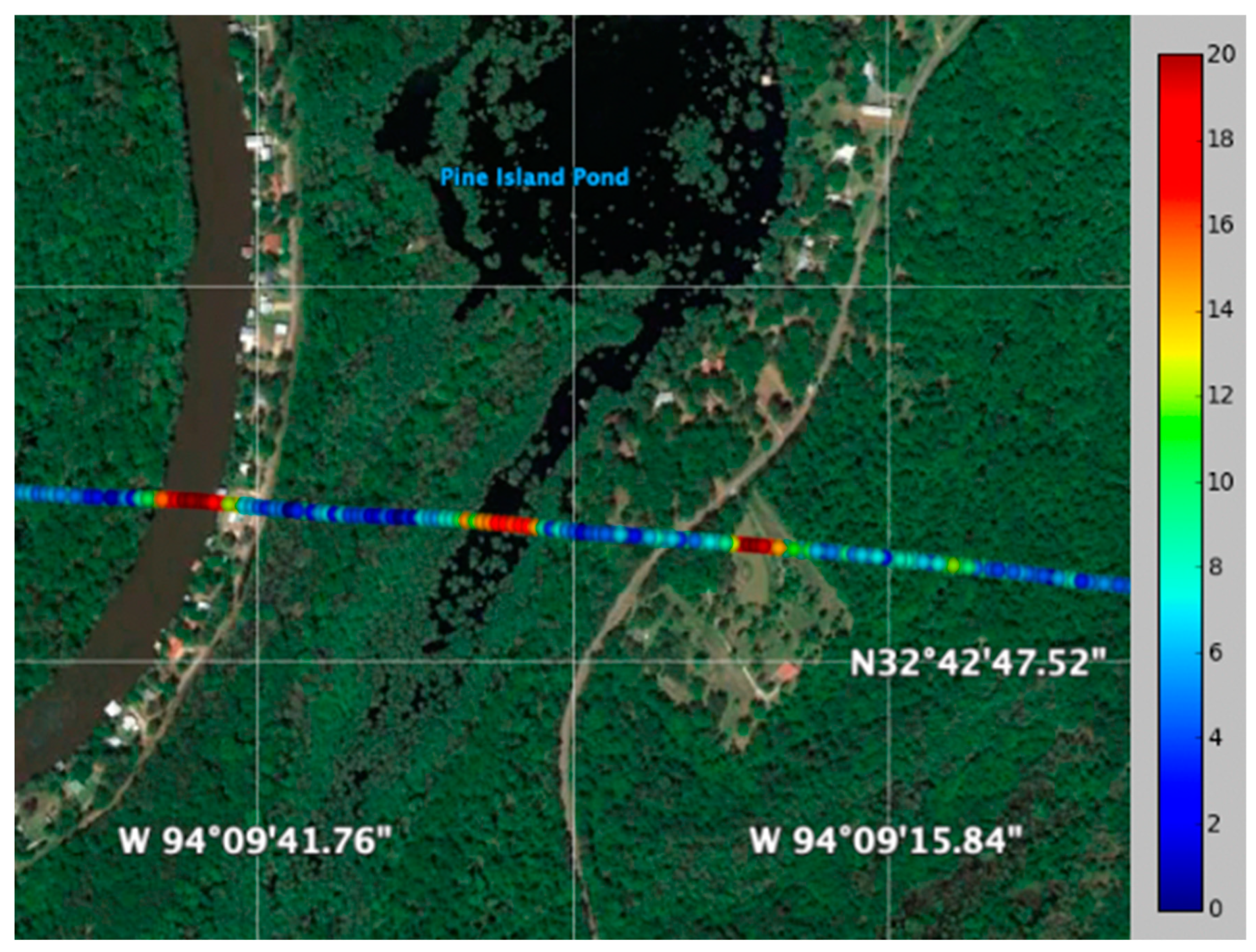
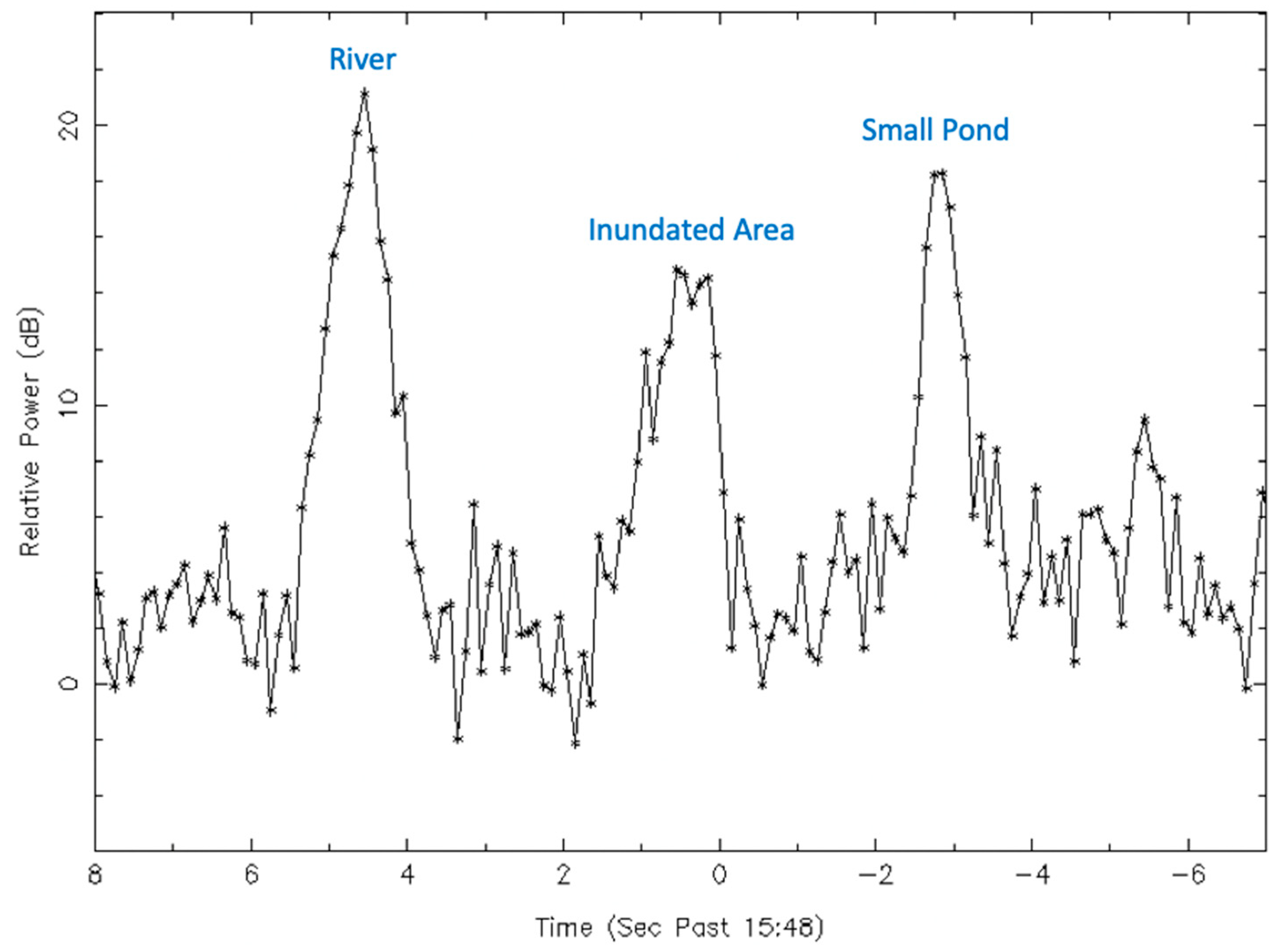
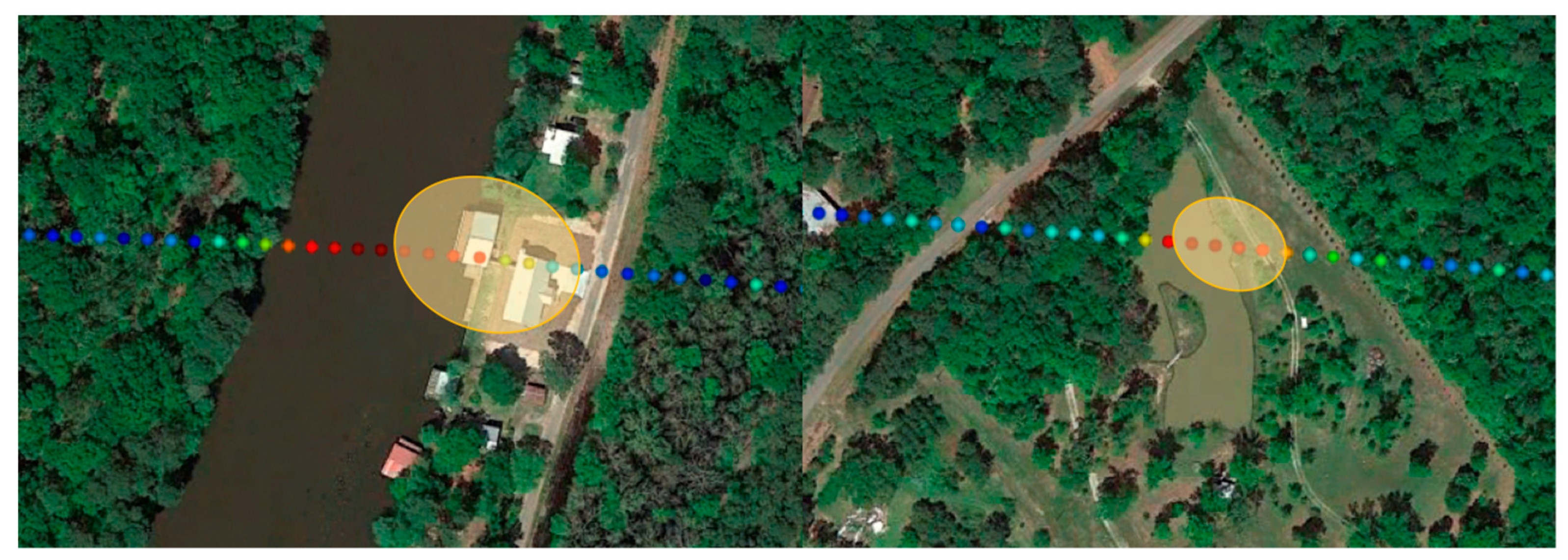
Figure 3 and Figure 4 show an example track over three bodies of water—a small pond, an inundated area, and a river. The track over the pond and river are reasonably clear and can be used to estimate the surface spot size, while the inundated area’s extent is uncertain due to overlying vegetation. The total duration of the pond and river crossings are approximately 0.8 s and 1.6 s, and their sizes under the track are about 31 m and 72 m, respectively. With an aircraft velocity of 81 m/s and assuming a simple boxcar (step-function) model for the spot, the spot size is estimated to be 34 m from the pond data and 58 m from the river data. This scene was chosen because it exemplifies the range of sizes deduced for essentially all the clear water transitions and crossings observed. Figure 5 shows a blowup of these crossings with their respective spot sizes indicated as yellow ellipses. The spots shown also account for the 33° incidence angle and the reflection plane being 170° CCW from the velocity vector. Both crossings have vegetation, flat open land, and/or buildings nearby, which can affect the measurements. With being within a few meters of 3130 m over this track, Equation (6) would predict the spot size along the track to be about 41 m, which is in good agreement with the observed values, given the boxcar model approximation and measurement uncertainties.
5.3. Caddo Lake
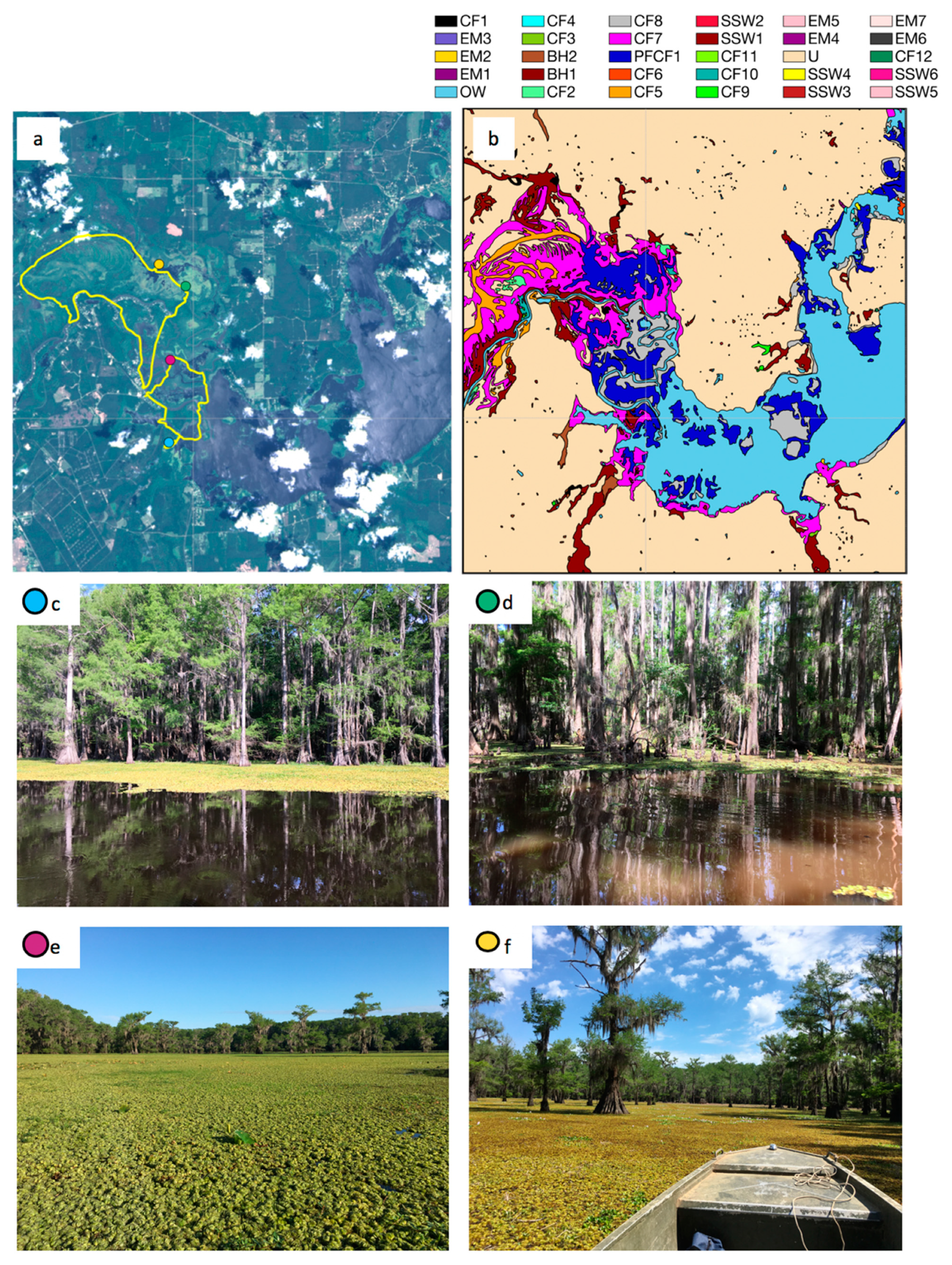
Figure 6a shows a pansharpened RGB image of the Caddo Lake area. Superimposed yellow lines are the paths the boat took concurrently with the GNSS-R flight. This region, the northwestern corner of Caddo Lake, is the area where inundated cypress forests are abundant. Giant Salvinia appears light green in the image shown in 6a.
Figure 6b shows a landcover classification map of Caddo Lake [22]. Abbreviated classes shown in legend are expanded in Table 1. The northwestern region of Caddo Lake contains a variety of intermittently, seasonally, semi-permanently, and permanently inundated cypress forests, scrub-shrub wetlands, and emergent species. The moving transient mats of giant Salvinia are not included in the landcover map. At the time of the aircraft experiment, they were prevalent predominantly in the areas denoted as permanently flooded cypress forests (PFCF1) but were also found in the semi-permanently flooded cypress forests (CF7/CF5), which can be seen in the Landsat 8 image in Figure 6a.
Selected photos depicting the conditions of Caddo Lake at the time of the aircraft experiment are shown in Figure 6c–e, and their respective locations are indicated by the colored dots in 6a. Figure 6c,d show typical cypress forests with a mixture of open water and giant Salvinia underneath the cypress trees. Figure 6e,f show two locations where giant Salvinia mats were particularly thick—the mats in 6f were thick enough to prevent further passage of the boat. Part of this analysis will show the effect of this aquatic vegetation on the ability for both C- and L-band signals to sense the underlying water.
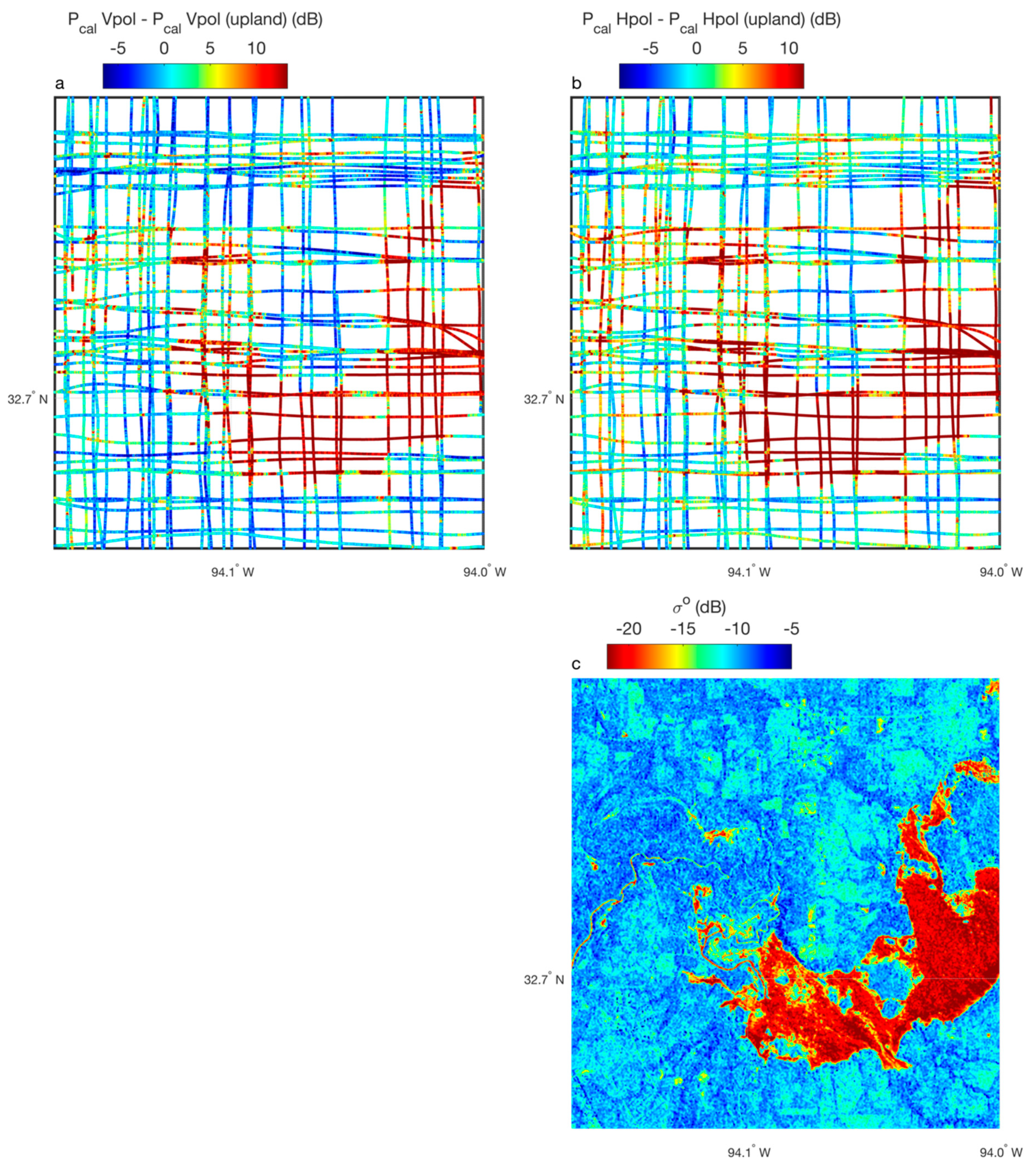
Figure 7 shows GNSS-R data (LHCP transmit, V pol received as well as LHCP transmit, Hpol received) collected during the flight experiment (a,b) and C-band data from Sentinel-1 (c; VV polarization). The Sentinel-1 data were collected on the same day as the Landsat image (Figure 6a), 8 May 2017. We do not expect there to have been significant variation in the inundated areas within and around Caddo Lake in the six days that spanned between the aircraft experiment and the acquisition date of the Sentinel-1 and Landsat data. Here, and in all figures that follow, we present the GNSS-R data as their values relative to their mean value over the upland landcover class (abbreviated U). In other words, we subtract the mean value obtained for observations falling over uplands from all observations. We do this in order to more clearly show the sensitivity of the GNSS-R signal to different wetland types. Overall, GNSS-R data from both V and H pol are very similar to one another, though on average the H pol data showed higher Equation (8)’s Pcal by 1.7 dB.
From Figure 7c, it is clear that the open water towards the eastern side of Caddo Lake is easily distinguishable in the Sentinel-1 data, apparent in the low sigma nought values. As stated above, low sigma nought values can indicate a very flat surface (e.g., smooth water) that results in little to no backscattering. As expected, the GNSS-R data in Figure 7a,b show the converse of this: the smooth open water on the eastern side of Caddo Lake produces high observed Pcal.
The northwestern side of Caddo Lake, with both cypress trees and giant Salvinia to obscure the water, is a more complex scattering environment. There is no qualitative distinction between the flooded cypress forests in the northwest and the surround upland areas, at least not as obvious of a distinction as that between the open water to the east and nearby uplands. There appears to be higher Pcal in the northwestern flooded forests relative to surrounding uplands, but without complete spatial sampling, this cannot be definitively concluded without a quantitative analysis.
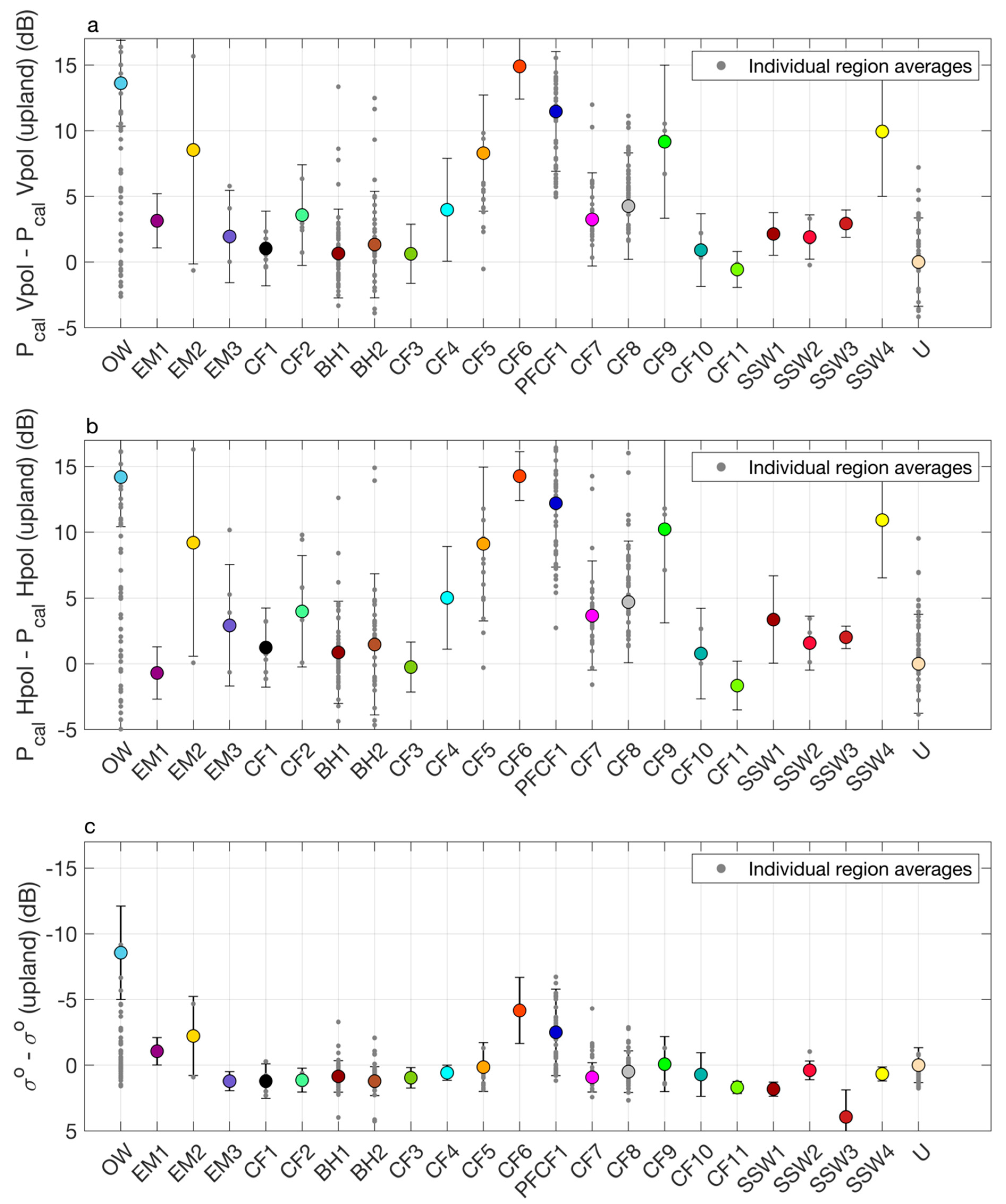
In order to quantify the sensitivity of both the GNSS-R aircraft data and that from Sentinel-1 to water obscured by vegetation, we first binned the observations by the landcover classes shown in Figure 6b. When binning the Sentinel-1 observations, we only used the data that corresponded to the locations where the GNSS-R data were collected, such that a direct comparison could be made. We calculated the mean and standard deviation of the sigma nought and Pcal observations within each landcover class, and we show this in Figure 8. For this analysis we again show GNSS-R data relative to its mean value over the upland land cover class, and now we show Sentinel-1 data also relative to its own mean value over uplands. Thus, for both the GNSS-R and Sentinel-1 data, the upland class (U) is plotted with a value of 0, and all other classes are relative to this value. Since results for the GNSS-R V- and H-pol data were so similar, the following results are described for only the V-pol data, though the H-pol data may be seen in Figure 8.
First, we focus on the sensitivity of the GNSS-R and Sentinel-1 data to the open water (OW) class, relative to uplands (U). Both show a several dB change between the classes: the mean increase in Pcal between uplands and open water was 13.61 dB, and the mean decrease in backscattering was 8.55 dB. In both the GNSS-R and Sentinel-1 data, the landcover class that came closest to open water was the intermittently exposed cypress forests (CF6). This type of landcover is only found in a very small portion of Caddo Lake—it is in the extreme northeastern part of the lake shown in Figure 3b. Although the sample size is small (n = 64), it appears that there is no attenuation of the GNSS-R signal through the vegetation canopy, as the observed mean Pcal was actually 1.29 dB higher than that observed over open water. This could indicate that the vegetation sheltered the water surface from any slight roughening from the wind, though given the relatively large standard deviation of the observations, the difference between open water and this vegetation class was small. The Sentinel-1 data show some attenuation through the vegetation, as there was a 4.4 dB increase in backscattering in the Sentinel-1 data.
Pcal over the permanently flooded cypress forests (PFCF1, n = 8345) also showed a high signal, only 2.15 dB lower than Pcal over open water. Sentinel-1 data over this landcover class was 6 dB higher than that over open water and 2.5 dB different than the backscattering over uplands. We attribute changes in the GNSS-R signal and Sentinel-1 data mostly to the presence of the giant Salvinia mats, and only partially to the presence of cypress trees in this class, as the spacing between the trees in this class is usually at least 50 m, which is more than the spatial resolution of both the GNSS-R and Sentinel-1 data. This indicates that there is some attenuation of the forward-scattered L-band signal through the giant Salvinia, but only 2.15 dB. For the backscattered C-band signal, the giant Salvinia geometry or biomass is not sufficient to produce a double bounced signal, but the vegetation itself is dense enough to produce significant backscatter, which makes the signal closer to that from upland rather than open water.
Another notable landcover class was the semi-permanently flooded cypress forests (CF5, n = 1781), which produced a Pcal of 8.3 dB higher than upland, and a sigma nought of 0.14 dB below the upland value. We again attributed this to the extensive presence of giant Salvinia in these areas at the time of acquisition.
In the densest cypress forests (CF8, n = 3816), we still saw a mean Pcal value 4.25 dB above the upland value, which was an indication that at least some of these forests were likely inundated. The sigma nought value was 0.5 dB higher than that for uplands. Despite the fact that parts of these forests were flooded, and the cypress trees having significant geometric components that might at L-band produce double bounce, it appeared that the C-band signals were not able to penetrate these types of canopies. Similar conclusions could be drawn for the other landcover classes in and around Caddo Lake.
The only notable distinction between the GNSS-R Pcal H-pol and V-pol data in terms of sensitivities to different landcover classes is the difference in mean Pcal over the EM1 landcover class (emergent reeds, semi-permanently flooded). In this case, the V-pol data show a few dB increase relative to the upland landcover class, whereas the H-pol data show a slight decrease relative to uplands. After closer examination, we found this single class to be misidentified, and instead of emergent reeds it should have been classified as uplands.
6. Discussion
Exploring the sensitivity of the GNSS-R signal to different wetland types based on a static landcover map is inherently an imperfect exercise. For example, just because the landcover map classifies an area as ‘semi-permanently flooded’ does not mean it actually was flooded during the flight experiment. Due to the extremely dense nature of the vegetation in Caddo Lake, it was not possible to conduct an extensive survey of flooded areas. In particular, we found many misclassifications of open water (OW) after comparing the Landsat 8 image and Google Earth images to the landcover classification map. These misclassifications were primarily small ponds to the north of Caddo Lake which had dried up or been converted to uplands in the time since the wetland inventory was conducted in 1983. These misclassifications can be seen in Figure 8, which also contains the mean Pcal value for individual landcover regions (i.e., each region classified as a particular landcover class instead of the class as a whole), indicated by the grey dots. Some individual regional averages for the open water (OW) class are quite low compared to the total average—these are the misclassified regions.
We plotted all individual region averages for each landcover class in Figure 8, not just for open water. For the most part, these regional averages cluster together, with individual region averages in the Sentinel-1 data mimicking what is observed in the GNSS-R data. A notable exception to the overall clustering of individual regions is for the EM2 (emergent reeds) class. In this case, there were two small clusters of observations over two different areas classified as EM2 in the southeast portion of Caddo Lake, separated by a larger region classified as CF7 (cypress forests). The cluster of observations closer to open water had a much higher mean Pcal V-pol than the cluster of observations adjacent to the upland/dry land. We interpret this as meaning that the cluster of observations in the EM2 region close to open water were probably responding to water underneath the reeds, whereas the reeds closer to the uplands/dry lands might have been dry. By considering these observations as being a part of one group only, a large standard deviation is the result.
7. Conclusions
From this aircraft experiment we have shown the scattering model in Equation (2) was appropriate for inundation and that the spot size in this case was approximately the Fresnel zone. From a comparison of L-band GNSS-R data with C-band Sentinel-1 data, we could conclude the following: The GNSS-R signal was able to penetrate the dense cypress canopies that typify Caddo Lake and other swamps in the southeast United States. There were several dB of attenuation, but the signal was still significantly higher than that over dry land. In addition, the presence of giant Salvinia only minimally attenuates the GNSS-R signal by ~2 dB. C-band backscatter data, on the other hand, was significantly attenuated by both of these vegetation types. This study was not able to conclude whether L-band backscatter signals, such as those collected by PALSAR-2, would be able to detect water underneath these types of vegetation, as there were no data publicly available. This study also did not quantify the saturation point for GNSS-R with respect to vegetation, as the GNSS-R signal was able to penetrate the vegetation canopies overflown here. Future GNSS-R aircraft flights, which could fly over denser vegetation canopies, might be able to quantify the saturation point, if there is one. Future studies should also focus on obtaining coincident L-band backscatter data, which could identify the relative strengths of the two data types without wavelength being a confounding factor.
Author Contributions
Conceptualization, S.T.L. and C.C.; methodology, S.T.L. and C.C.; experiment hardware, S.T.L., J.S. and M.K.; antenna calibration, S.T.L., J.S. and M.K.; data-collection software, J.S. and M.K.; experiment campaign, S.T.L., J.S. and C.C; analysis software, S.T.L.; validation, S.T.L and C.C.; formal analysis, S.T.L. and C.C.; resources, S.T.L., C.C., J.S. and M.K.; data curation, S.T.L., J.S. and M.K.; writing—original draft preparation, S.T.L. and C.C.; writing—review and editing, S.T.L. and C.C.; supervision, S.T.L.; project administration, S.T.L.; funding acquisition, S.T.L. All authors have read and agreed to the published version of the manuscript.
Funding
This research was carried out at the Jet Propulsion Laboratory, California Institute of Technology, under a contract with the National Aeronautics and Space Administration (NASA). Support for this work was provided by NASA’s Solid Earth Program, JPL’s Research and Technology Development Program, and JPL’s Advanced Concepts Program. Part of this work was funded by NASA NNH17ZDA001N-THP. © 2020. All rights reserved.
Acknowledgments
We thank Keystone Arial Surveys, Inc. for excellent performance and handling the 2-year flight delay, members of the Caddo Lake Institute for their information on this region, Dr. Roy Darville of East Texas Baptist University for providing a boat tour around Caddo Lake, JPL’s Bruce Haines for processing the aircraft Novatel data through Gipsy, and JPL’s Larry Young for his help with the antenna calibration experiment.
Conflicts of Interest
The authors declare no conflict of interest. The funders had no role in the design of the study; in the collection, analyses, or interpretation of data; in the writing of the manuscript, or in the decision to publish the results.
References
- Stocker, T.F.; Qin, D.; Plattner, G.-K.; Tignor, M.; Allen, S.K.; Boschung, J.; Nauels, A.; Xia, Y.; Bex, V.; Midgley, P.M. (Eds.) IPCC, 2013: Climate Change 2013: The Physical Science Basis. Contributions of Working Group I to the Fifth Assessment Report of the Intergovernmental Panel on Climate Change; Cambridge University Press: Cambridge, UK; New York, NY, USA, 2013. [Google Scholar]
- Melton, J.R.; Wania, R.; Hodson, E.L.; Poulter, B.; Ringeval, B.; Spahni, R.; Bohn, T.; Avis, C.A.; Beerling, D.J.; Chen, G.; et al. Present state of global wetland extent and wetland methane modelling: Conclusions from a model inter-comparison project (WETCHIMP). Biogeosciences 2013, 10, 753–788. [Google Scholar] [CrossRef] [Green Version]
- Ringeval, B.; de Noblet-Ducoudré, N.; Ciais, P.; Bousquet, P.; Prigent, C.; Papa, F.; Rossow, W.B. An attempt to quantify the impact of changes in wetland extent on methane emissions on the seasonal and interannual time scales. Glob. Biogeochem. Cycles 2010, 24, GB2003. [Google Scholar] [CrossRef] [Green Version]
- Shindell, D.T.; Walter, B.P.; Faluvegi, G. Impacts of climate change on methane emissions from wetlands. Geophys. Res. Lett. 2004, 31, 21. [Google Scholar] [CrossRef]
- Catry, T.; Li, Z.; Roux, E.; Herbreteau, V.; Gurgel, H.; Mangeas, M.; Seyler, F.; Dessay, N. Wetlands and Malaria in the Amazon: Guidelines for the Use of Synthetic Aperture Radar Remote-Sensing. Int. J. Environ. Res. Public Health 2018, 15, 368. [Google Scholar] [CrossRef] [PubMed] [Green Version]
- Gopal, B. Future of wetlands in tropical and subtropical Asia, especially in the face of climate change. Aquat. Sci. 2013, 75, 39–61. [Google Scholar] [CrossRef]
- Pekel, J.F.; Cottam, A.; Gorelick, N.; Belward, A.S. High-resolution mapping of global surface water and its long-term changes. Nature 2016, 540, 418–422. [Google Scholar] [CrossRef] [PubMed]
- Schroeder, R.; McDonald, K.; Chapman, B.; Jensen, K.; Podest, E.; Tessler, Z.; Bohn, T.; Zimmermann, R. Development and evaluation of a multi-year fractional surface water data set derived from active/passive microwave remote sensing data. Remote Sens. 2015, 7, 16688–16732. [Google Scholar] [CrossRef] [Green Version]
- Du, J.; Kimbal, J.; Galantowicz, J.; Kim, S.; Chan, S.; Reichle, R.; Jones, L.; Watts, J. Assessing global surface water inundation dynamics using combined satellite information from SMAP, AMSR2 and Landsat. Remote Sens. Environ. 2018, 213, 1–17. [Google Scholar] [CrossRef] [PubMed]
- Martinez, J.M.; le Toan, T. Mapping of flood dynamics and spatial distribution of vegetation in the Amazon floodplain using multitemporal SAR data. Remote Sens. Environ. 2007, 108, 209–223. [Google Scholar] [CrossRef]
- Nghiem, S.V.; Zuffada, C.; Shah, R.; Chew, C.; Lowe, S.; Mannucci, A.; Cardellach, E.; Brakenridge, G.; Geller, G.; Rosenqvist, A. Wetland monitoring with global navigation satellite system reflectometry. Earth Sp. Sci. 2017, 4, 16–39. [Google Scholar] [CrossRef] [PubMed]
- Jensen, K.; McDonald, K.; Podest, E.; Rodríguez-Álvarez, N.; Horna, V.; Steiner, N. Assessing L-band GNSS-Reflectometry and Imaging Radar for Detecting Sub-Canopy Inundation Dynamics in a Tropical Wetlands Complex. Remote Sens. 2018, 10, 1431. [Google Scholar] [CrossRef] [Green Version]
- Rodriguez-Alvarez, N.; Podest, E.; Jensen, K.; McDonald, K. Classifying Inundation in a Tropical Wetlands Complex with GNSS-R. Remote Sens. 2019, 11, 1053. [Google Scholar] [CrossRef] [Green Version]
- Morris, M.; Chew, C.; Reager, J.T.; Shah, R.; Zuffada, C. A novel approach to monitoring wetland dynamics using CYGNSS: Everglades case study. Remote Sens. Environ. 2019, 233, 111417. [Google Scholar] [CrossRef]
- Zribi, M.; Motte, E.; Baghdadi, N.; Baup, F.; Dayau, S.; Fanise, P.; Guyon, D.; Huc, M.; Wigneron, J. Potential Applications of GNSS-R Observations over Agricultural Areas: Results from the GLORI Airborne Campaign. Remote Sens. 2018, 10, 1245. [Google Scholar] [CrossRef] [Green Version]
- Egido, A.; Paloscia, S.; Motte, E.; Guerriero, L.; Pierdicca, N.; Caparrini, M.; Santi, E.; Fontanelli, G.; Floury, N. Airborne GNSS-R polarimetric measurements for soil moisture and above-ground biomass estimation. IEEE J. Sel. Top. Appl. Earth Obs. Remote Sens. 2014, 7, 1522–1532. [Google Scholar] [CrossRef]
- Chew, C.C.; Small, E.E. Soil Moisture Sensing Using Spaceborne GNSS Reflections: Comparison of CYGNSS Reflectivity to SMAP Soil Moisture. Geophys. Res. Lett. 2018, 45, 4049–4057. [Google Scholar] [CrossRef] [Green Version]
- Chew, C.C.; Shah, R.; Zuffada, C.; Hajj, G.; Masters, D.; Mannucci, A.J. Demonstrating soil moisture remote sensing with observations from the UK TechDemoSat-1 satellite mission. Geophys. Res. Lett. 2016, 43, 3317–3324. [Google Scholar] [CrossRef] [Green Version]
- Comite, D.; Ticconi, F.; Dente, L.; Guerriero, L.; Pierdicca, N. Bistatic Coherent Scattering from Rough Soils with Application to GNSS Reflectometry. IEEE Trans. Geosci. Remote Sens. 2019, 58, 612–625. [Google Scholar] [CrossRef]
- Ulaby, F.; Moore, R.; Fung, A. Microwave Remote Sensing: Active and Passive; Addison-Wesley Publishing Company: Boston, MA, USA, 1982; p. 02116. [Google Scholar]
- Stefanski, J. Step by Step: Recommended Practice Flood Mapping. UN-SPIDER Knowledge Portal. 2015. Available online: http://www.un-spider.org/ (accessed on 2 September 2019).
- Data Server for Caddo Lake Information. 2017. Available online: http://caddolakedata.us/maps (accessed on 9 September 2019).
- Camps, A. Spatial Resolution in GNSS-R Under Coherent Scattering. IEEE Geosci. Remote Sens. Lett. 2019, 17, 1–5. [Google Scholar] [CrossRef]
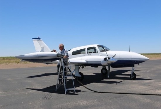
Figure 1.
(a) Keystone’s Cessna 310 used for all three flights. (b): Antenna calibration experiment.
Figure 1.
(a) Keystone’s Cessna 310 used for all three flights. (b): Antenna calibration experiment.

Figure 2.
(a): Sampler and front-end electronics (top) with 8 antenna inputs and low-noise amplifiers (LNAs), and solid state disk (SSD) array (bottom) with 8 TB of storage. (b): View of 9-element patch antenna from inside the aircraft, with central three patches’ H and V-Pol outputs cabled. IR camera is on upper left of antenna, and optical camera is small black box on lower left of antenna.

Figure 3.
Westward ground track near Caddo Lake of PRN 23 over a Google Earth image from April 2017. The track’s calibrated power in dBs is color coded from low to high as blue to red respectively, over a 20-dB range.
Figure 3.
Westward ground track near Caddo Lake of PRN 23 over a Google Earth image from April 2017. The track’s calibrated power in dBs is color coded from low to high as blue to red respectively, over a 20-dB range.

Figure 4.
Received power vs. time corresponding to the westward ground track in Figure 3. Note that time increases to the left to align with Figure 3 features. Points are 0.1 s apart, and the aircraft velocity was 81 m/s.

Figure 5.
Blowup of the pond (right) and river (left) crossings from Figure 3, with yellow ellipses indicating the approximate orientation and size of the surface spot size, as derived from their respective power measurements vs time.
Figure 5.
Blowup of the pond (right) and river (left) crossings from Figure 3, with yellow ellipses indicating the approximate orientation and size of the surface spot size, as derived from their respective power measurements vs time.

Figure 6.
(a) Pansharpened Landsat 8 image of Caddo Lake from 8 May 2017. Yellow lines are GPS tracks of the boat. Colored dots are locations of photos in (c–f). (b). Landcover classification map of Caddo Lake [22]. Acronyms are defined in Table 1.

Figure 7.
(a) Global Navigation Satellite System-Reflectometry (GNSS-R) Equation (8)’s Pcal Vpol observations over Caddo Lake, acquired on 2 May 2017. Observations are relative to their mean value over uplands (156.63 dB). (b) Same as (a), except showing GNSS-R Pcal Hpol observations, relative to their mean value over uplands (158.39 dB). (c) Sigma nought observations (VV pol) from Sentinel-1, acquired on 8 May 2017.

Figure 8.
(a) Mean GNSS-R Pcal Vpol observation, binned by the landcover classes in the Caddo Lake area, defined in Table 1. Error bars are ± one standard deviation. Observations are relative to the mean value over uplands (U), which was 156.63 dB. (b) Same as (a) except for GNSS-R Pcal Hpol observations (mean value over uplands = 158.39 dB). (c) Same as (a) except for sigma nought observations from Sentinel-1. The mean value over uplands (U) was -10.4 dB. Individual region averages are shown by the grey dots.


Table 1.
Landcover classification abbreviations used in this study. General and specific classes and the wetland ID follow conventions found in [22].
Table 1.
Landcover classification abbreviations used in this study. General and specific classes and the wetland ID follow conventions found in [22].
| Abbreviation | General Class | Specific Class | Wetland ID |
|---|---|---|---|
| OW | open water | open water | L1UBHh |
| EM1 | emergents | emergent reeds, semipermanently flooded | PEM5/FLCh |
| EM2 | emergents | emergent reeds, permanently flooded | PEM5/UBFH |
| EM3 | emergents | emergent reeds, seasonally flooded | PEM5C |
| CF1 | cypress forests | broad-leaved deciduous, scrub-shrub temporarily flooded | PFO/SS1A |
| CF2 | cypress forests | needle-leaved deciduous, scrub-shrub semipermanently flooded | PFO/SS2F |
| BH1 | bottomland hardwoods | broad-leaved deciduous, temporarily flooded | PFO1A |
| BH2 | bottomland hardwoods | broad-leaved deciduous, seasonally flooded | PFO1C |
| CF3 | cypress forests | needle-leaved deciduous, semipermanently flooded | PFO2/1F |
| CF4 | cypress forests | needle-leaved deciduous, seasonally flooded | PFO2/UBCh |
| CF5 | cypress forests | needle-leaved deciduous, semipermanently flooded | PFO2/UBF |
| CF6 | cypress forests | needle-leaved deciduous, intermittently exposed | PFO2/UBG |
| PFCF1 | permanently flooded cypress forests | needle-leaved deciduous, permanently flooded | PFO2/UBH |
| CF7 | cypress forests | needle-leaved deciduous, semipermanently flooded | PFO2F |
| CF8 | cypress forests | needle-leaved deciduous, intermittently exposed | PFO2Gh |
| CF9 | cypress forests | dead forest, permanently flooded | PFO5/UBHh |
| CF10 | cypress forests | deciduous, temporarily flooded | PFO6A |
| CF11 | cypress forests | deciduous, seasonally flooded | PFO6C |
| SSW1 | scrub-shrub wetlands | scrub-shrub broad-leaved deciduous, temporarily flooded | PSS1A |
| SSW2 | scrub-shrub wetlands | scrub-shrub broad-leaved deciduous, seasonally flooded | PSS1C |
| SSW3 | scrub-shrub wetlands | scrub-shrub broad-leaved deciduous, semipermanently flooded | PSS1F |
| SSW4 | scrub-shrub wetlands | scrub-shrub needle-leaved deciduous, permanently flooded | PSS2/UBHh |
| U | upland | upland | U |
| EM4 | emergents | emergent reeds, evergreen semipermanently flooded | PEM5/AB7F |
| EM5 | emergents | emergent reeds, temporarily flooded | PEM5A |
| SSW5 | scrub-shrub wetlands | scrub-shrub, needle-leaved deciduous intermittently exposed | PSS2/UBG |
| SSW6 | scrub-shrub wetlands | scrub-shrub, broad-leaved deciduous semipermanently flooded | PSS1/EMFh |
| CF12 | cypress forests | broad-leaved deciduous, seasonally flooded | PFO/SS1C |
| EM6 | emergents | emergent persistent semipermanently flooded | PEM1Fh |
| EM7 | emergents | emergent reeds semipermanently flooded | PEM5Fh |
© 2020 by the authors. Licensee MDPI, Basel, Switzerland. This article is an open access article distributed under the terms and conditions of the Creative Commons Attribution (CC BY) license (http://creativecommons.org/licenses/by/4.0/).
Share and Cite
MDPI and ACS Style
Lowe, S.T.; Chew, C.; Shah, J.; Kilzer, M. An Aircraft Wetland Inundation Experiment Using GNSS Reflectometry. Remote Sens. 2020, 12, 512. https://0-doi-org.brum.beds.ac.uk/10.3390/rs12030512
AMA Style
Lowe ST, Chew C, Shah J, Kilzer M. An Aircraft Wetland Inundation Experiment Using GNSS Reflectometry. Remote Sensing. 2020; 12(3):512. https://0-doi-org.brum.beds.ac.uk/10.3390/rs12030512
Chicago/Turabian StyleLowe, Stephen T., Clara Chew, Jesal Shah, and Michael Kilzer. 2020. "An Aircraft Wetland Inundation Experiment Using GNSS Reflectometry" Remote Sensing 12, no. 3: 512. https://0-doi-org.brum.beds.ac.uk/10.3390/rs12030512
Note that from the first issue of 2016, this journal uses article numbers instead of page numbers. See further details here.