Combining Spectral Unmixing and 3D/2D Dense Networks with Early-Exiting Strategy for Hyperspectral Image Classification


1
School of Computer Science, National Engineering Laboratory for Integrated Aero-Space-Ground-Ocean Big Data Application Technology, Shaanxi Provincial Key Laboratory of Speech Image & Information Processing, Northwestern Polytechnical University, Xi’an 710129, China
2
School of Computing and Information Systems, The University of Melbourne, Melbourne, VIC 3010, Australia
*
Author to whom correspondence should be addressed.
Remote Sens. 2020, 12(5), 779; https://0-doi-org.brum.beds.ac.uk/10.3390/rs12050779
Submission received: 14 December 2019
/
Revised: 26 February 2020
/
Accepted: 27 February 2020
/
Published: 29 February 2020
Abstract
:Recently, Hyperspectral Image (HSI) classification methods based on deep learning models have shown encouraging performance. However, the limited numbers of training samples, as well as the mixed pixels due to low spatial resolution, have become major obstacles for HSI classification. To tackle these problems, we propose a resource-efficient HSI classification framework which introduces adaptive spectral unmixing into a 3D/2D dense network with early-exiting strategy. More specifically, on one hand, our framework uses a cascade of intermediate classifiers throughout the 3D/2D dense network that is trained end-to-end. The proposed 3D/2D dense network that integrates 3D convolutions with 2D convolutions is more capable of handling spectral-spatial features, while containing fewer parameters compared with the conventional 3D convolutions, and further boosts the network performance with limited training samples. On another hand, considering the existence of mixed pixels in HSI data, the pixels in HSI classification are divided into hard samples and easy samples. With the early-exiting strategy in these intermediate classifiers, the average accuracy can be improved by reducing the amount of computation cost for easy samples, thus focusing on classifying hard samples. Furthermore, for hard samples, an adaptive spectral unmixing method is proposed as a complementary source of information for classification, which brings considerable benefits to the final performance. Experimental results on four HSI benchmark datasets demonstrate that the proposed method can achieve better performance than state-of-the-art deep learning-based methods and other traditional HSI classification methods.
1. Introduction
Hyperspectral Image (HSI) comprise hundreds of narrow and contiguous spectral bands, and each represents the measured intensity of a narrower range of light frequencies [1]. The great spectral resolution of HSI improves the capability of precisely discriminating the surface materials of interest [2,3]. Such abundant spectral information makes it beneficial to a wide range of applications, especially in some cases that cannot be directly detected by humans. For most of these applications, HSI classification has been an active area of research in remote sensing research. Abundant spectral resolution is useful for classification problems but at the expense of much lower spatial resolution. Because of the low spatial resolution of HSI, the spectral signature of each pixel contains a mixture of different spectra, which is caused by the multiple components that form the ground surface materials. If a pixel is highly mixed in HSI data, it is very difficult to categorize it in the original feature space. Therefore, the presence of mixed pixels is one of the major obstacles affecting seriously the classifier accuracy [4].
In recent years, in HSI data analysis, the spectral unmixing techniques [5] have been employed to handle with the mixed pixel issue. The spectral unmixing includes two steps: (1) extracting the pure material spectra (endmembers) from the HSI and (2) calculating their relative proportions (abundances) of the HSI data [6]. Spectral unmixing has been extensively studied as a possible solution in HSI analysis. Related research works and applications have been developed in many fields, such as HSI super-resolution, denoising, change detection, and so on [7,8,9]. For instance, in Reference [7], Lanaras et al. proposed a method which performs hyperspectral super-resolution by jointly coupled spectral unmixing. The proposed joint formulation significantly improves hyperspectral super-resolution. Yang et al. [8] proposed a sparse representation framework that unifies denoising and spectral unmixing in a closed-loop manner. This method utilizes spectral information from spectral unmixing as feedback to correct spectral distortion, while denoising and spectral unmixing act as constraints to iteratively solve other constraints. In Reference [9], a general framework for HSI change detection using sparse unmixing is proposed. This model has the potential to get more information than other change detection techniques.
Moreover, spectral unmixing also carries valuable information for the HSI classification problem. A brief review of existing HSI classification methods with spectral unmixing is given below. Generally, these algorithms can be divided into two groups. Firstly, spectral unmixing has been widely studied as a feature extraction strategy before classification [10,11,12,13]. For instance, in Reference [10], unmixing results is used to improve classification performance in an alternative strategy and spectral unmixing can be used to extract suitable features for future classify images. Later, Dópido et al. [11] quantitatively evaluated the unmixing-based feature extraction methods, and further proved that these features can effectively improve the accuracy of classification. This strategy was further explored in many works [12,13] and also proved that the unmixing before classification provided an effective solution for HSI classification. Secondly, several techniques are proposed to utilize the complementarity of the classification and spectral unmixing in a semi-supervised framework, where the abundance maps have been applied as a supplementary source for the multinomial logistic regression (MLR) classifier [14,15,16,17]. First, the framework utilizes the information provided by spectral unmixing to select new training samples for classification, and then it integrates the abundance maps and classification to obtain the final classification results. This strategy considers the output provided by both classification and unmixing simultaneously, which provides a joint approach for HSI interpretation and can effectively improve the classification results, particularly when the available training set is very limited.
More recently, the deep learning-based methods have shown state-of-the-art performance in HSI classification [18,19,20,21,22], thanks to its great success in computer vision and the fast advancement of computing facilities [23,24,25,26,27]. Instead of shallow manually-crafted features, deep learning network models can extract high-level, hierarchical and abstract features which are generally more robust to nonlinear processing. In Reference [18], Pan et al., proposed a simplified deep learning model called R-VCANet [18] (vertex component analysis network) based on the deep learning baseline PCANet [27]. In recent studies, convolutional neural networks (CNNs) [23] are most often used in deep learning-based methods for HSI classification [19,20,21]. For example, a 3D CNN based on the 3D convolutional kernel is proposed in Reference [19], and the discriminative spectral-spatial features and classification are performed in an end-to-end manner. Zhong et al. [20] proposed a supervised spectral-spatial residual network (SSRN) based on the residual neural network (ResNet) [24]. An SSRN consists of consecutive spectral and spatial residual blocks, which are used to extract spectral-spatial features of HSI.
Furthermore, dense convolutional networks (DenseNet) have demonstrated significant achievement in deep learning network models and have also been used for HSI classification [28,29,30], particularly in limited training samples, because the dense connections have a regularizing effect, which reduces overfitting on tasks with smaller training set sizes [31]. In Reference [21], a 3D dense convolutional network with multiple scales dilated convolutions [32] and a spectral-wise attention mechanism (MSDN-SA) is proposed for HSI classification with limited training samples. The 3D CNN has a very important characteristic, that is they can directly create hierarchical representations of spectral-spatial data. However, the number of parameters grows exponentially when convolution goes from 2D to 3D. Due to the additional kernel dimension, 3D network has more parameters than 2D CNN. A large number of parameters make it easily prone to over-fitting when there are only limited labeled samples. Besides, when the 3D network is applied to HSI classification, the power of 3D network comes at a considerable cost, namely the computational cost of applying them to new examples. It is necessary to design a network model for resource-efficient HSI classification with limited training samples [33].
Considering the successful combination of HSI unmixing and classification, as well as the development of deep learning, we aimed at integrating spectral unmixing with deep learning-based classification algorithm to improve the classification accuracy. Little research has been undertaken on the combining of these two techniques. Recently, Alam et al. [12] used spectral unmixing to generate abundance maps and then used abundance maps as the input for deep learning-based HSI classification. However, in some cases, it is important to take advantage of the unmixing and classification information in a complementary manner, but the algorithm [12] uses the information provided by spectral separation before classification [15].
Based on the above motivations, a novel 3D/2D dense network where multiple intermediate classifiers are integrated with the spectral unmixing method for HSI classification is proposed. For HSI data with mixed pixels, compared with state-of-the-art CNN, this model shows its superiority in terms of overall classification accuracy, especially in limited training samples. The three contributions of this paper can be summarized as follows.
- Our model adopts a specially designed network with multiple intermediate classifiers that is trained end-to-end. A 3D/2D dense networks with multiple intermediate classifiers (3D/2DNets) are jointly optimized during training and early-exiting strategy is adopted for each sample during testing. This is a resource-efficient model concerning other deep learning-based HSI classifiers.
- We proposed a spectral-spatial 3D/2D convolution (SSDC) for the proposed framework. It enables the network to incorporate fewer 3D convolutions, while taking advantage of 2D convolutions to obtain more spectral information feature maps and enhance feature learning capabilities, thereby reducing the training complexity of each round of spectral-spatial fusion, which reduces overfitting on tasks with limited training samples.
- An adaptive spectral unmixing is proposed as a complementary source for classification. The endmember composition of each pixel is established by the probabilistic output of softmax adaptively.
2. Proposed Methods
2.1. Overview
The proposed method aims to learn an early-exiting deep learning framework for HSI classification based on 3D/2D dense networks (denoted as 3D/2DNets) and adaptive spectral unmixing (ASU). The whole framework is abbreviated as ASU-3D/2DNets. We exploit the fact that HSI data is typically a combination of easy examples and hard examples. Based on the above facts, a 3D/2D dense network with early-exiting strategy is proposed, which can reduce the evaluation time without loss of accuracy. Furthermore, considering the pixels with a low probabilistic output are either mixed pixels or pixels that are difficult to classify due to spectral variability, we unmix the hard samples to get more accurate classification results.
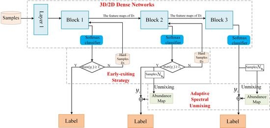
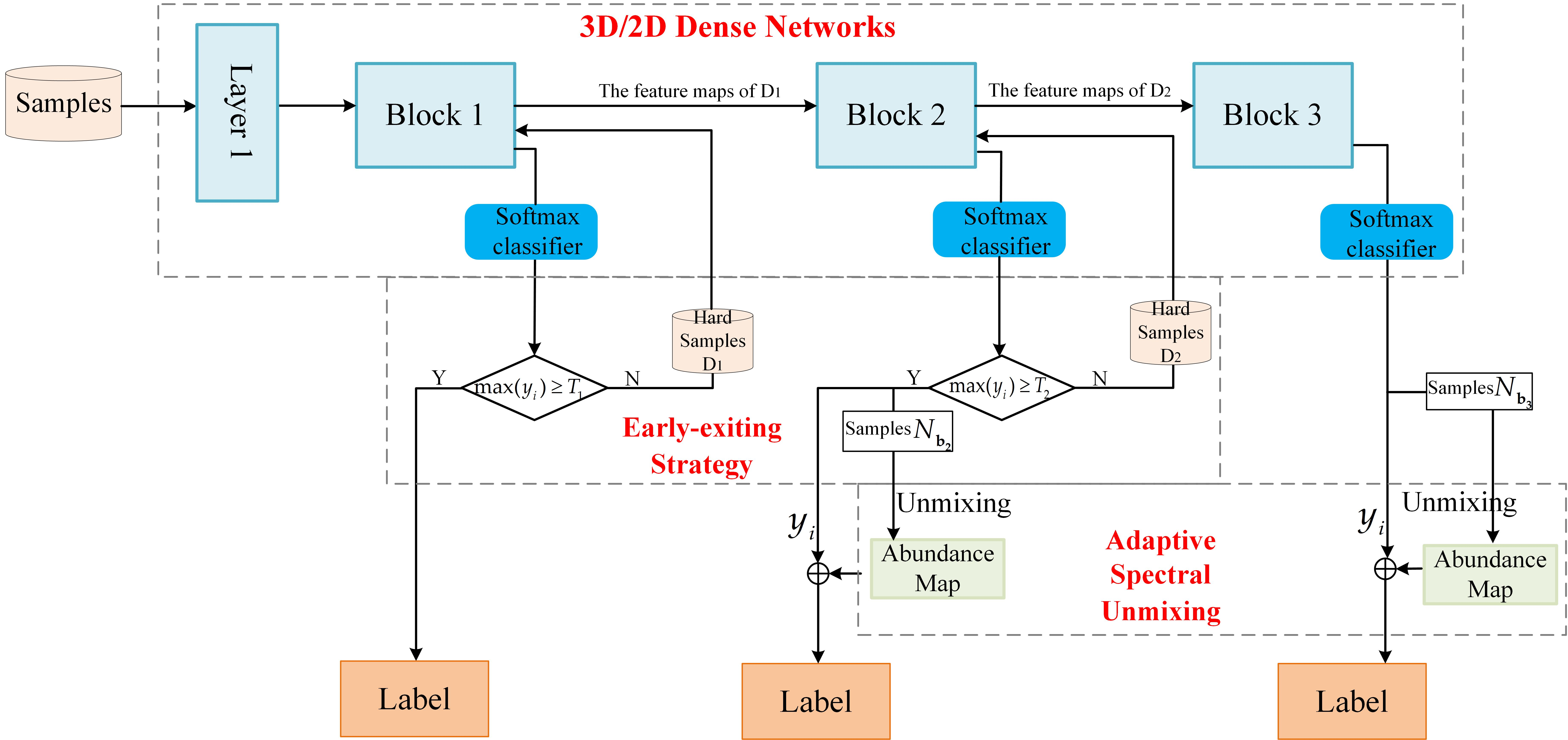
The framework of the proposed method is shown in Figure 1. All available labeled samples are divided into three parts: training samples, validation samples, and testing samples. The method is mainly composed of three parts: 3D/2D dense networks; early-exiting strategy; and adaptive spectral unmixing.
3D/2D dense networks: To be specific, the 3D/2D dense networks composed of one convolution layer and three blocks, each block is connected to a classifier exit. In training processing, a 3D/2D dense network with multiple intermediate classifiers is jointly optimized.
Early-exiting strategy: Considering the existence of mixed pixels in HSI, the pixels in HSI classification can be divided into hard samples and easy samples. We intend to prioritize easy samples from early layer and difficult to classify samples (hard samples) from later layers. This process is called the early-exit strategy. All samples first pass the Block 1, each sample can be assigned to a class and the probability of each sample in the softmax layer is denote as , where , , i is the number of categories. If the softmax probability value of samples obtained in the classification process is greater than a chosen threshold , the system sends them down to exit; otherwise, it sends the samples (the hard samples ) to the Block 2. After the samples pass through the Block 2, if the softmax probability value of samples obtained in the classification process is greater than a chosen threshold , the system will send them to exit and future unmix them. Otherwise, the samples (the hard samples ) will be input into the Block 3 to continue to extract deeper features. The samples output from each block is represented as , , and , respectively.
Adaptive spectral unmixing: At the exit of the Block 2, by considering the results of the coarse classification step and applying the fully constrained least squares (FCLS) [34] method to each unlabeled pixel, spectral unmixing is performed to the unclassified pixels to obtain the abundance maps. As a result, abundance maps provide additional information about the composition of each pixel. Finally, the contribution degree of abundance maps and classification results are controlled by weight, and the final classification map is obtained.
Next, we will detail the 3D/2D dense networks with early-exiting strategy and adaptive spectral unmixing.
2.2. 3D/2D Dense Networks with Early-Exiting Strategy
Recently, two-dimensional multi-scale dense networks (MSDNets) is first proposed for resource-efficient image classification [35]. MSDNets uses a cascade of intermediate early-exiting classifiers throughout the network. In these intermediate early-exiting classifiers setting, MSDNets can improve the average accuracy by reducing the amount of computation spent on easy samples to save up computation for hard samples [35].
Based on the fact of that HSI data is typically a mix of easy examples and hard examples, we are trying to apply MSDNets to the HSI classification, thereby increasing the classification accuracy whilst reducing the computational requirements. As HSI data are 3D cubes, it is reasonable to extend the 2D model to the 3D model for HSI classification; however, greatly increasing on both computational complexity and memory usage has followed. To resolve this problem, an early-exiting dense network with mixed 3D and 2D convolutions (3D/2DNets) is proposed. In this section, we first give a detailed description of early-exiting dense networks. Then, a 3D/2D convolution based on spectral and spatial information is presented for early-exiting dense networks.
2.2.1. Dense Networks Architecture with Early-Exiting Strategy
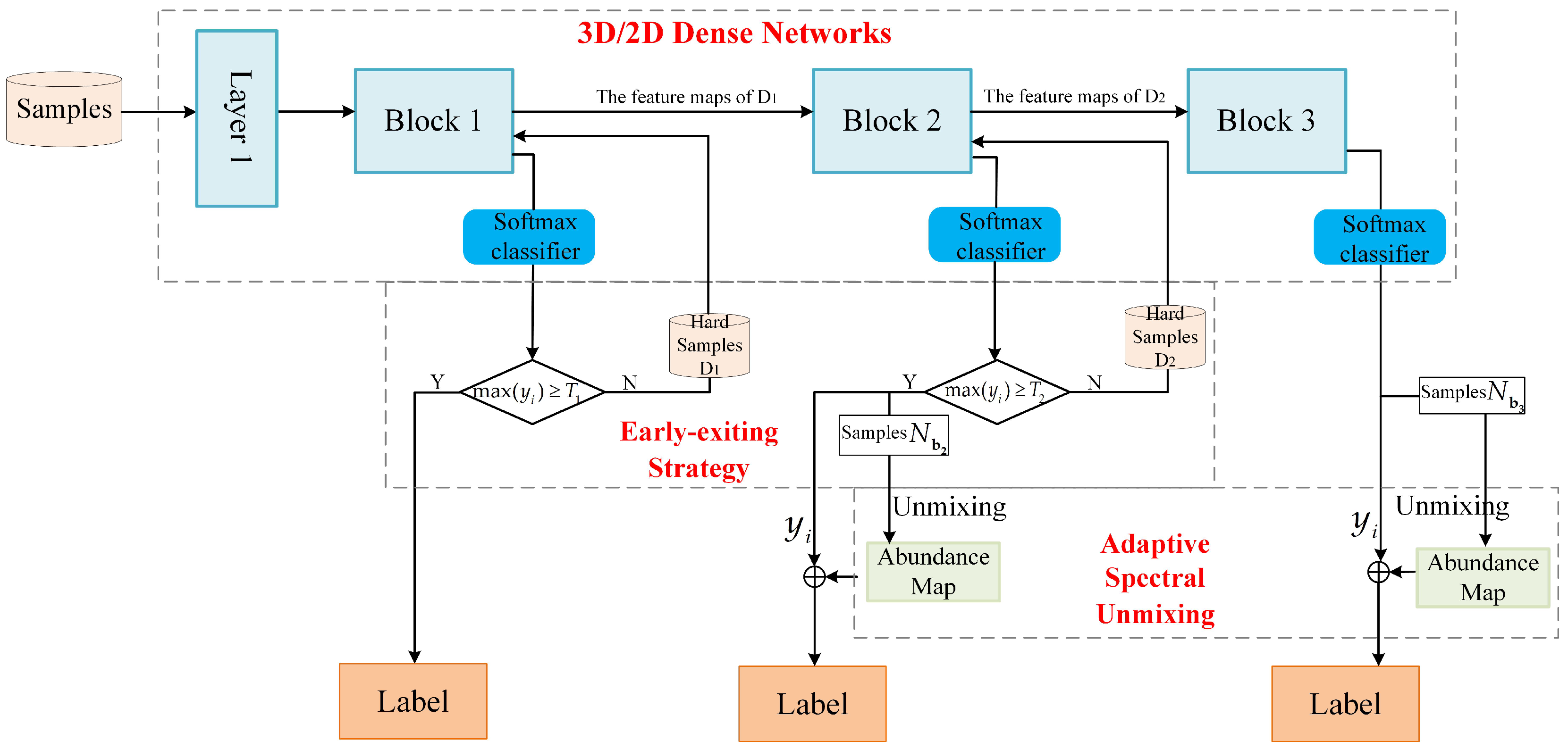
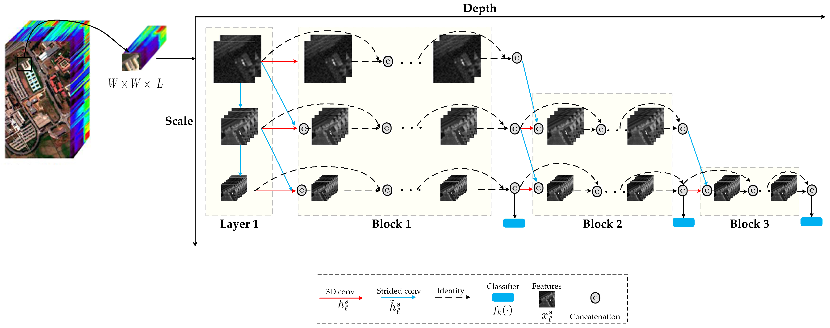
Figure 2 gives an illustration of the dense networks architecture with early-exiting strategy. As shown, the network is based on DenseNets [31] and cascaded intermediate early-exiting classifiers throughout the network. Because coarse-scale features are important to classify the content of the sample patch into a single class, the network maintains a feature representation at multiple scales throughout the network, and all the classifiers only use the coarse-level features. We perform the early-exiting of the easy examples at early classifiers whilst propagating hard examples through the entire network, using the procedure described in Section 2.1.
In sample extraction, we extract cube with the size , where W and L are the spatial size and the number of spectral bands, respectively. Each cube is extracted from a neighborhood window centered around a pixel, and the label of each sample is that of the pixel located in the center of this cube. Then, we feed 3D cube into the multi-scale dense networks model, which is itself composed of one convolution layer and three blocks, to obtain the classification result.
- (1)
- The convolutional layer functions in the first layer ( ), ; denote a sequence of -sized 3D convolutions (Conv), the batch normalization layer with rectified linear unit (ReLU) function, and a 3D max pooling layer with -sized kernel, stride of 2. The output feature maps at ℓ layer and scale s are denoted as .
- (2)
- For subsequent feature layers in each block, the transformations and are defined following the design in DenseNets [32]: Conv()-BN-ReLU-Conv()-BN-ReLU. We set the number of output channels of the three scales to 6, 12, and 24, respectively. The output feature maps produced at subsequent layers, and scales s, are a concatenation of transformed feature maps from all previous feature maps of scale s and (if ).
- (3)
- Each classifier has two down-sampling convolutional layers with 128 dimensional filters, followed by a 3D average pooling layer and a linear layer. The classifier at layer ℓ uses all the features . Let denote the k th classifier, every sample traverses the network and exits after classifier if its prediction confidence (we use the maximum value of the softmax probability as a confidence measure) exceeds a pre-determined threshold T.
During training, we use cross entropy loss functions for all classifiers and minimize a cumulative loss as follows:
where D denotes the training set.
2.2.2. 3D/2D Convolutional Based on Spectral-Spatial Information
In HSI classification, a 3D convolution couples spectral-spatial information to effectively extract spectral-spatial features. Though promising, regarding 2D CNN, 3D CNN extends the spatial kernel to spectral-spatial space, which significantly increase the number of parameters, thus greatly increasing the computational complexity and memory usage, as well as increasing the network’s demand for huge training sets [36]. It can be seen from the above analysis that the above facts limit the performance of existing 3D CNN on HSI classification, especially in dense convolution networks based on 3D convolution [21]. There are currently some efforts to ameliorate the downside of the 3D convolution model in HSI classification. Zhong et al. [20] first employed the style of residual connection to extract the spectral features by continuous 1D convolution, and then used 3D convolution to extract spatial information. Furthermore, in Reference [37], the combination of a 2D spatial convolution and a 1D spectral convolution was used to replace spectral-spatial 3D convolution, which means that this network structure was no longer 3D CNN.
Recently, intertwined 3D/2D networks [38,39,40] have shown up as a hybrid between 2D CNN and 3D CNN in human action recognition. In Reference [38], a mixed convolutional tube (MiCT) was proposed to integrate 2D convolution with the 3D convolution to learn better spatio-temporal features. Compared to the 3D CNN, a benefit of using such 3D/2D networks is that the parameters involved in the networks are much reduced.
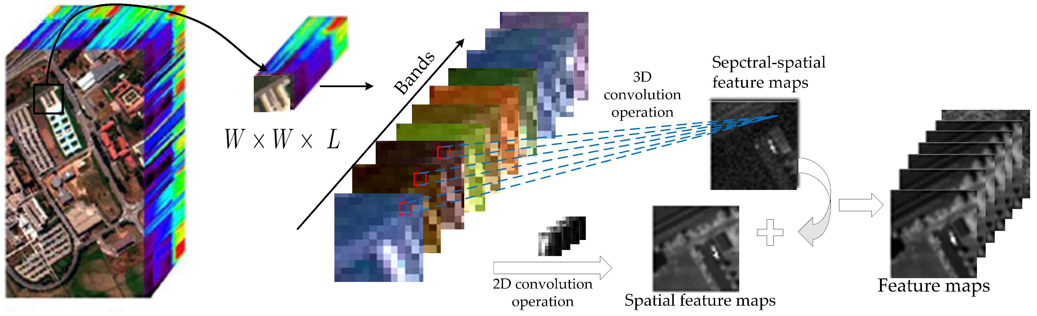
Inspired by this, to alleviate the drawback of 3D convolution in the HSI classification, inspired by Reference [38], we proposed a spectral-spatial 3D/2D convolution (SSDC) for HSI, as illustrated in Figure 3. The SSDC replaces each 3D convolution in the first layer of the proposed framework. Considering the HSI data has a lot of redundant spectral information among consecutive bands, this results in redundant information in feature maps along the spectral dimension. In the first layer, if all the bands are directly used in the network input, the 3D sample block will input too many parameters and increase the computational complexity. Therefore, the proposed SSDC is used to replace the 3D convolution used in the first layer network. It enables the network to incorporate fewer 3D convolutions, while taking advantage of 2D convolutions to obtain more spectral information feature maps and enhance feature learning capabilities, thereby reducing the training complexity of each round of spectral-spatial fusion, which reduces overfitting on tasks with limited training samples.
The shortcut in our SSDC is cross-domain [38] is different from the residual connections in previous works [21,24]. The SSDC is obtained by 3D convolution mapping for the 3D inputs and a 2D convolution mapping for the 2D inputs. By introducing a 2D convolution to extract the 2D features information on each band, the 3D convolution in SSDC only needs to learn residual information along the spectral dimension. Thus, the cross-domain residual connection largely reduces the complexity of SSDC in 3D convolution kernels learning.
2.3. An Adaptive Endmember Selection of Unmixing
As described above, the method of combining classification and unmixing has achieved good results in pixel labeling, in which the abundance maps have been used as an auxiliary information source in the MLR classifier [10,11,16]. However, all the above methods process all pixels in the same way, but the fact that hyperspectral data is that some samples may be not highly mixed (in this case, the coarse classification step may be sufficient to characterize them), and some samples may be highly mixed (in this case, spectral unmixing is particularly useful for enhancing the classification) [15]. With the aforementioned issues in mind, adaptive spectral unmixing is introduced to the 3D/2D dense networks with early-exiting classifier. Through this network architecture, the easy examples were correctly classified and exited by the first classifier. The examples with low probabilistic outputs are either mixed pixels or pixels hard to classify due to spectral variability; we unmix the hard samples to achieve more accurate classification results. In general, adaptive spectral unmixing consists of two important parts, the collection of endmembers spectrum and adaptive endmember selection.
Firstly, in our framework, the spectral signatures used for unmixing purposes are not obtained by endmember extraction but are obtained by averaging the spectral signatures of each labeled category in the training set. Although the average endmembers will cause a decrease in spectral purity, it can reduce the effects of noise and/or average the subtle spectral variability of each spectral category, resulting in a more representative final endmember as a whole [10,13].
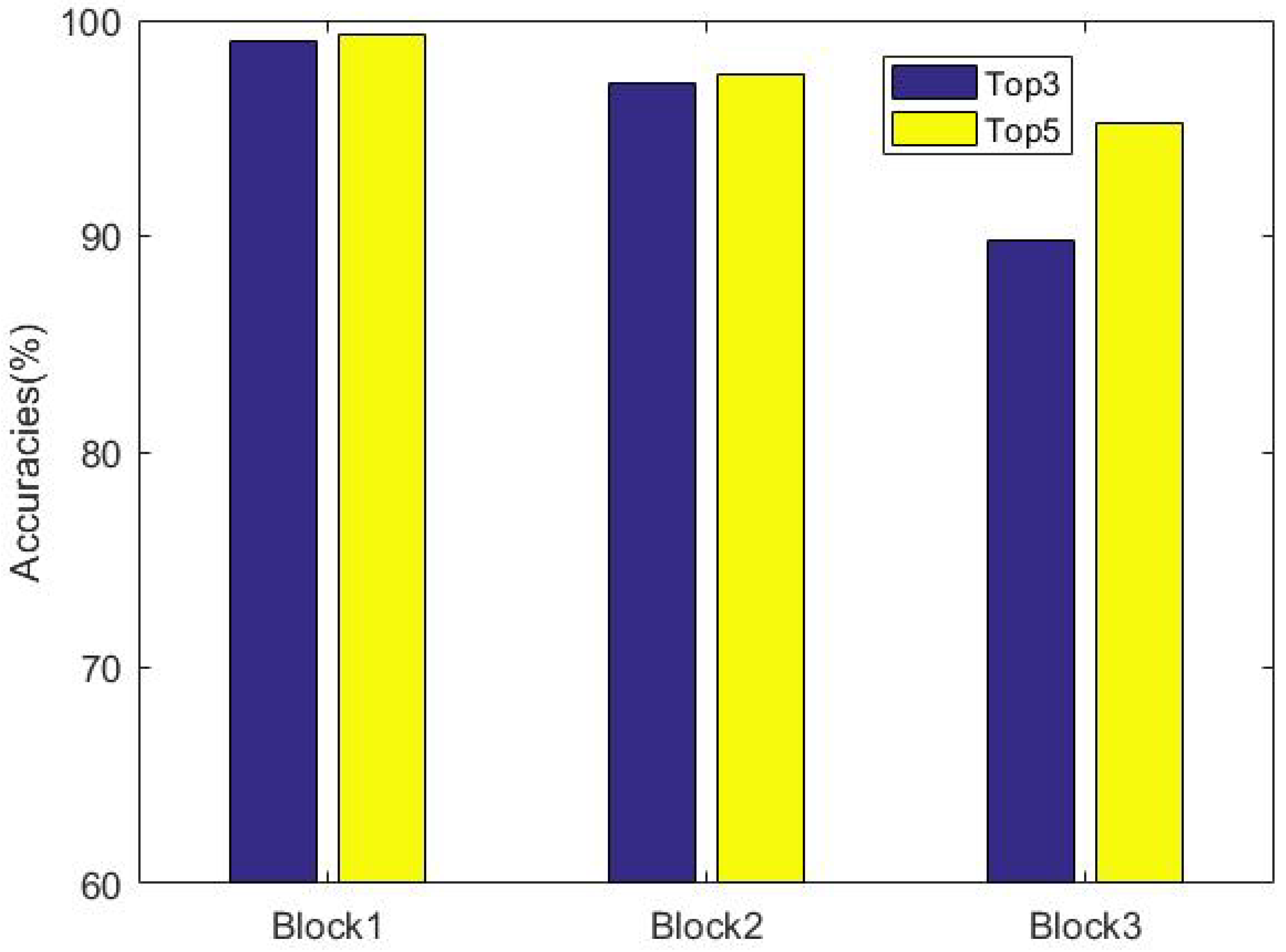
In the spectral unmixing of mixed pixels, the choice of endmembers is extremely important. We did a simple experiment, and Figure 4 shows the classification results of each block output. In Figure 4, we find the hard samples (maybe highly mixed), which are from the second and third classifiers, and the probabilistic output of top3—the top3 value refers to the top three in the maximum probability vector. As long as the correct probability is present, the prediction is correct; otherwise, the prediction error is close to 99% in second classifiers, and the probabilistic output of top5 is also 95% in third classifiers. So, we speculate that the endmember composition of a mixed pixel can represent its main component with a few endmembers instead of all endmembers, and according to the different spectral purity, different processing strategies should be adopted for different types of the pixel. This theory has also been verified in the literature [15]. Therefore, we propose an endmember selection of unmixing in which the probabilistic output of softmax is exploited to determine the endmember set for each pixel.
To be specific, all samples first pass the first block, and every sample can be assigned to a class. If the probabilistic output obtained in the classification process is greater than a chosen threshold T ( and ), the system sends it down to exit; otherwise, it sends the sample to the second block. It is worth mentioning that the easy examples were correctly classified and exited directly by the first classifier. For each sample output from the second classifier, we take the top3 result of the corresponding probabilistic output as the endmember, and for the sample output by the third classifier, we take the top5 of the probabilistic output classification result as the endmember.
where is the selected endmember set of sample i from the k th classifier. If , then ; if , then . denotes endmember set.
Lastly, the adaptive endmembers are adopted for the fully constrained least squares (FCLS) [34] unmixing model. As a result, abundance map provides additional information about the composition of each pixel. Finally, the contribution degree of abundance map and classification result is controlled by weight , and the final classification map is obtained as follows:
where function is the probability obtained by the classification algorithm, i.e., the kth classifier described in Section 2.2.1; and function is the abundance fraction obtained by the spectral unmixing with adaptive endmember .
3. Experimental Results and Discussion
3.1. Experimental Data Sets
In this section, one synthetic dataset and four benchmark HSI datasets, including Indian Pines, Salinas Valley, Kennedy Space Center (KSC), and Pavia University, are used to evaluate the performance of the proposed method. The first three datasets were collected by the NASA Airborne Visible/Infrared Imaging spectrometer (AVIRIS) instrument; the last one was collected by the ROSIS-03 sensor.
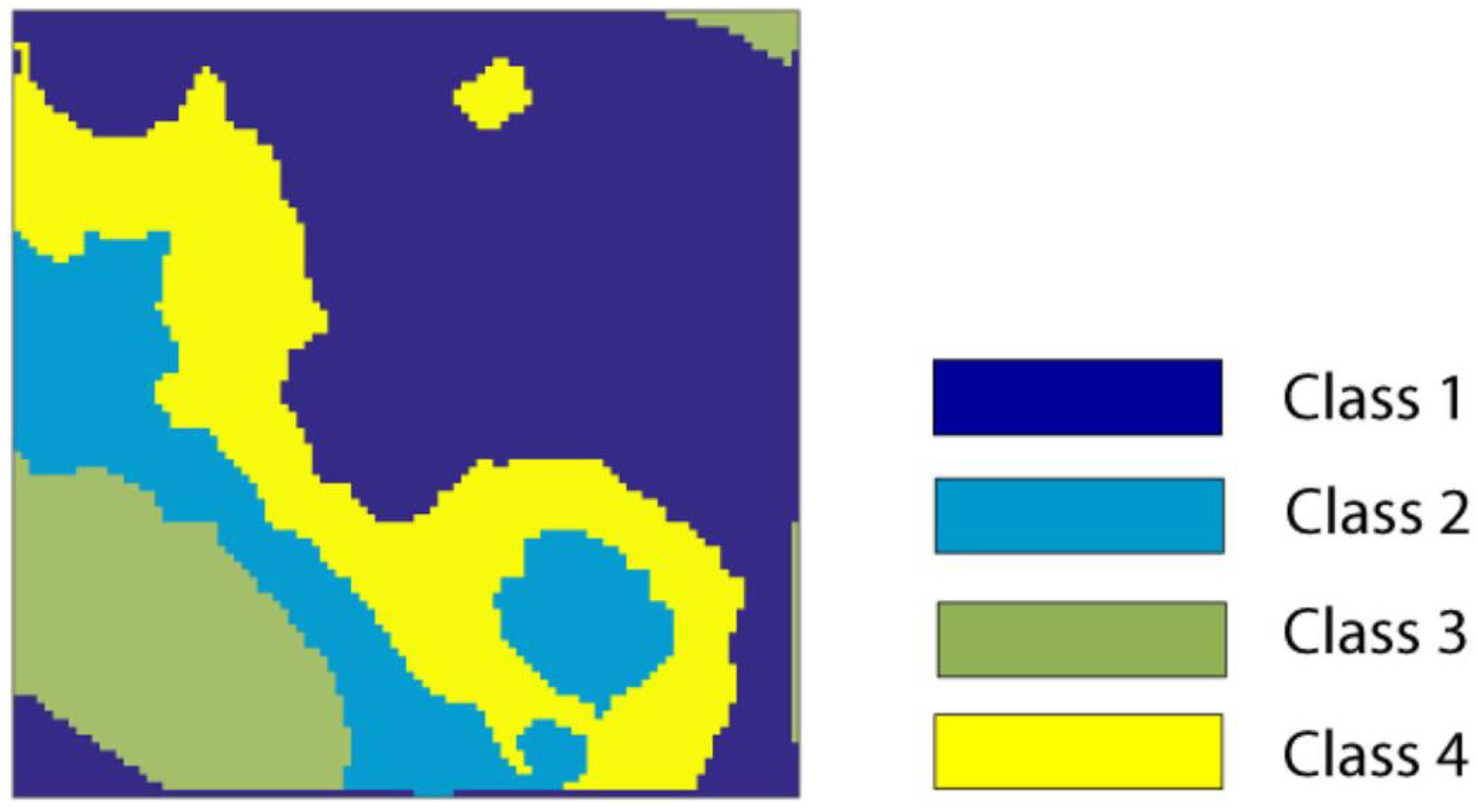
To assess the classification performance in a totally controlled environment, we generate synthetic datasets of four classes (see Figure 5). It should be noted that the proposed approach exploits the linear mixture model. Let be the i th samples in class k,
where are pure spectra from the U.S. Geological Survey digital spectral library, is the corresponding abundance fraction, and is the number of constituents in class k. For a certain sample , we assume that receives the maximum abundance value, which, in turn, determines the corresponding label . The zero-mean Gaussian noise is also added to the pixel .
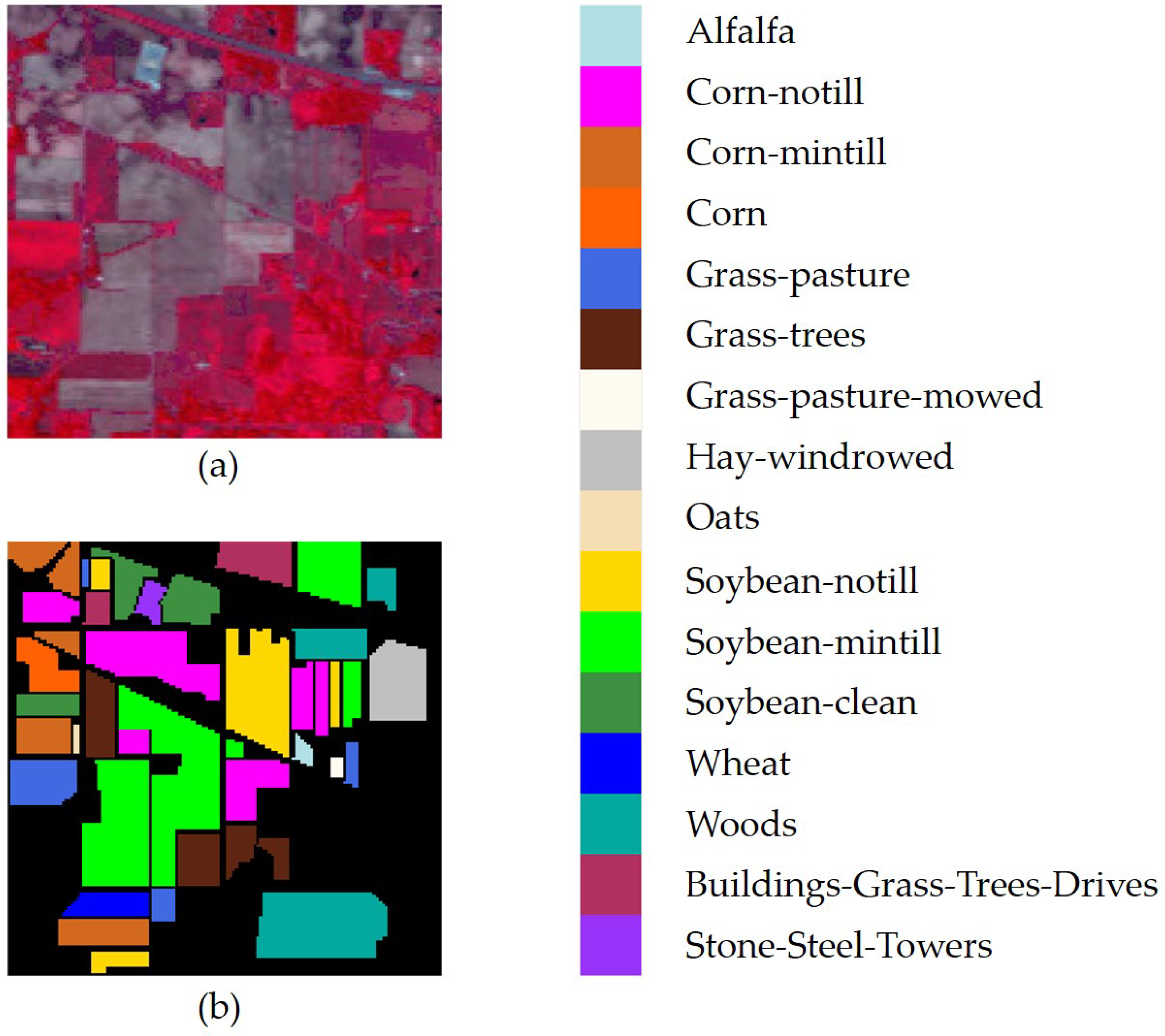
The Indian Pines image was recorded by the AVIRIS sensor over the Indian Pines test site in Northwestern Indiana, with 20 m spatial resolution and 0.4–2.5 m wavelength range. It consists of pixels and 220 spectral reflectance bands. Twenty spectral bands (104–108,150–163, and 220) were removed due to the noise and water absorption, and the remaining 200 bands image was used as the original for the experiments reported herein. The ground-truth data contains 16 classes, the false color composite image and the reference map are shown in Figure 6a,b, respectively.
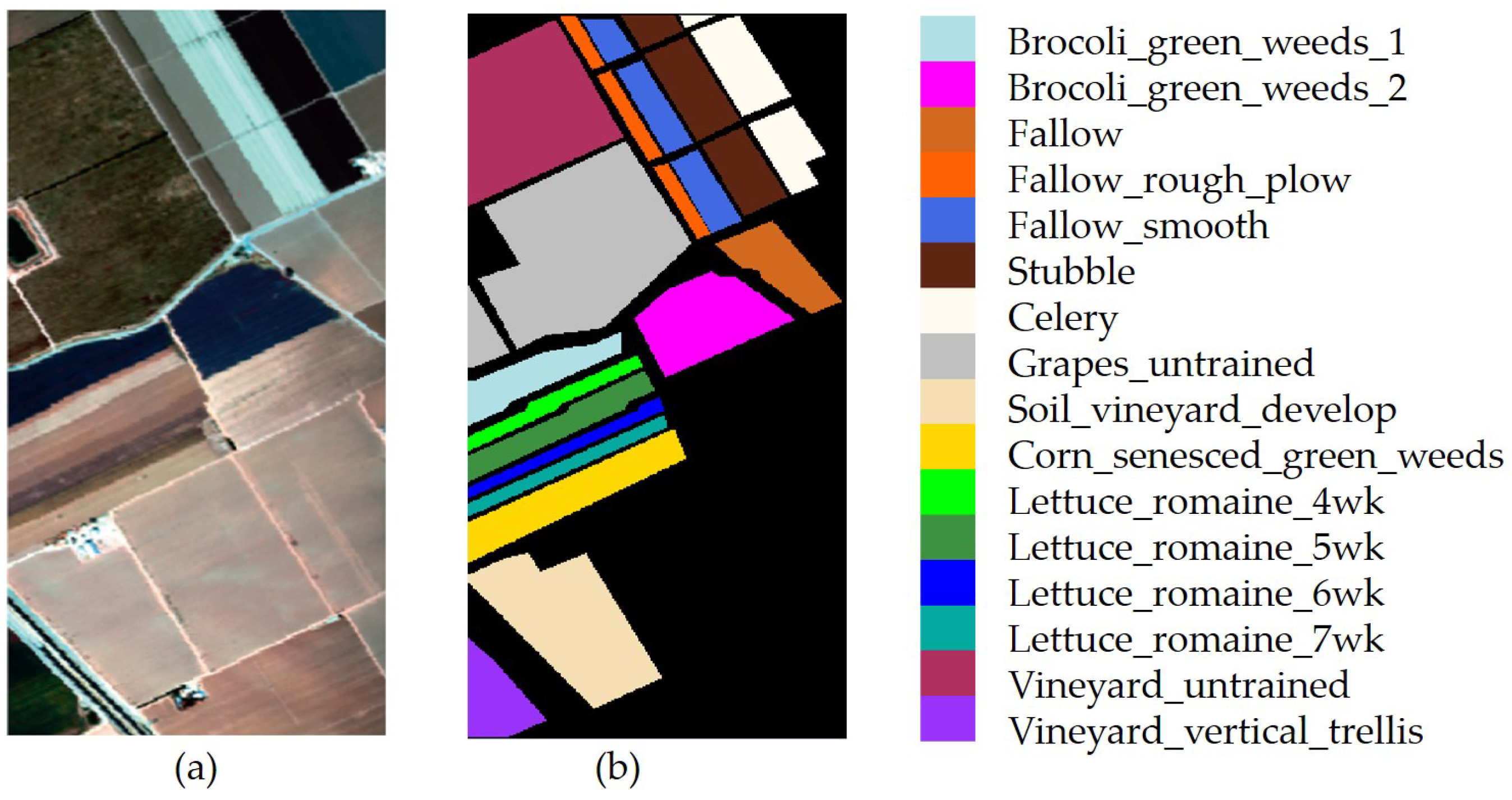
The Salinas Valley image was captured by the AVIRIS sensor over Salinas Valley, California, and is characterized by 3.7 m spatial resolution. It consists of pixels and 224 spectral bands and 0.4–2.5 m wavelength range, where twenty water absorption bands (108–112, 154–167, and 224) were removed. The reference image contains 16 land-cover classes. Figure 7a,b shows the true color composite of the Salinas Valley image and the corresponding reference data.
The KSC image was recorded by the AVIRIS sensor over the KSC site in Florida, with 18 m spatial resolution and 0.4–2.5 m wavelength range. After removing water absorption and low signal-to-noise-ratio (SNR) bands, the remaining 176 bands and pixels are used for assessment. Training data were selected using land cover maps derived from color infrared photography provided by the KSC and Landsat Thematic Mapper (TM) imagery. The vegetation classification scheme was developed by KSC personnel in an effort to define functional types that are discernible at the spatial resolution of Landsat and these AVIRIS data. Discrimination of land cover for this scene is difficult due to the similarity of spectral signatures for certain vegetation types. For classification purposes, 13 upland and wetland classes representing the various land cover types that occur in this scene were defined for the site. Figure 8a,b shows the true color composite of the KSC image and the corresponding reference data.
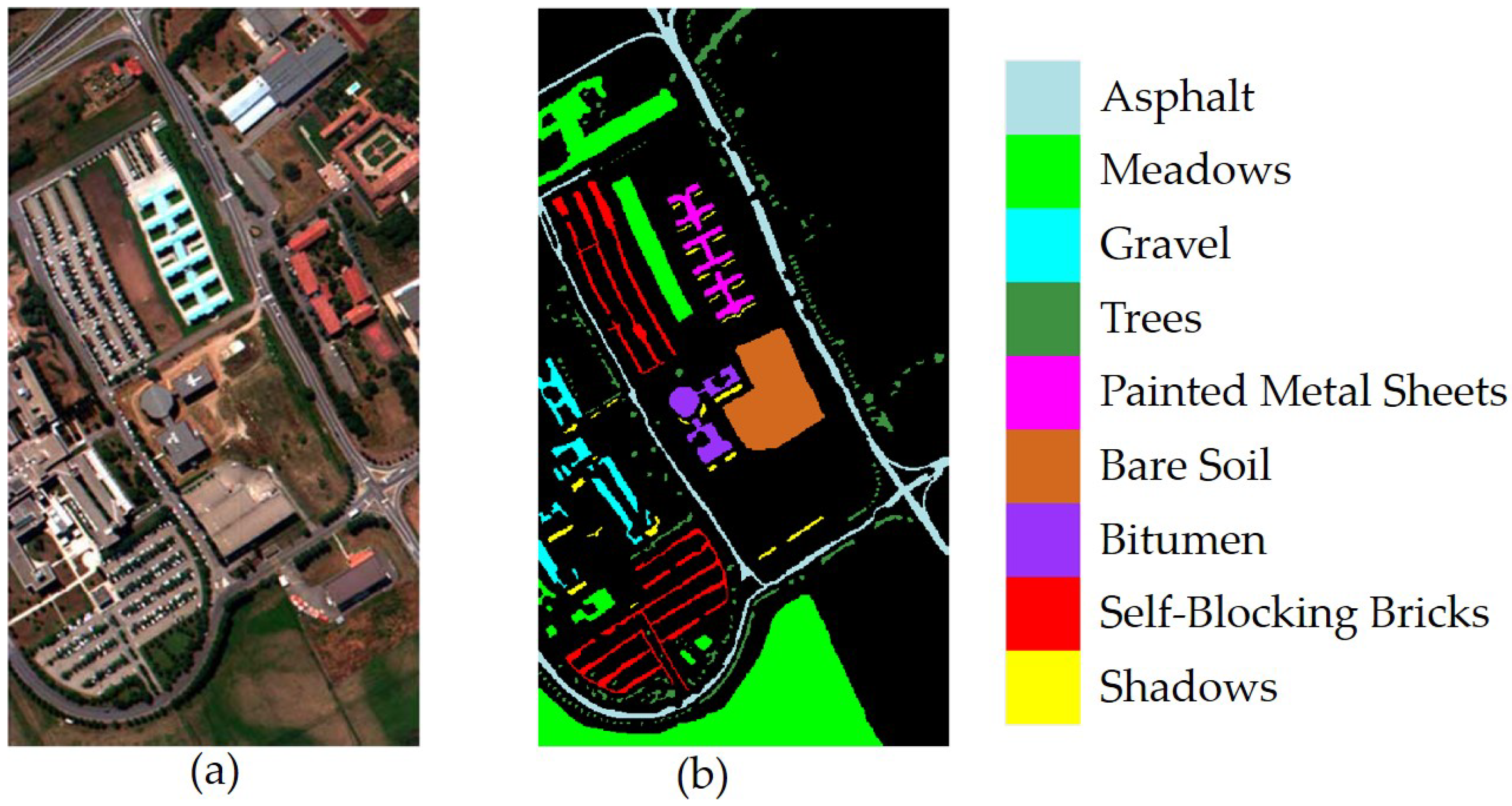
The Pavia University image was gathered by the ROSIS sensor during a flight campaign over Pavia, northern Italy, having pixels with 1.3 m spatial resolution. It consists of 115 spectral bands at the range 0.43–0.86 m. Twelve spectral bands were removed due to noise, and the remaining 103 bands were used for classification of nine classes. The true color composite of the Pavia University image and the corresponding reference image are shown in Figure 9a,b, respectively.
3.2. Experimental Settings
All the compared methods are assessed numerically using the following three criteria: overall accuracy (OA), average accuracy (AA), and statistically kappa coefficient (). We implemented 10 trials of hold-out cross validation for each dataset: the mean values and standard deviations are reported for each dataset. For each trial, a limited number of training samples were randomly selected from each class, 10% of the labeled samples are chosen as validation samples, and the remaining samples were used as testing samples. The training samples are used to train the weights and biases of each neuron in the model, while the architecture variables are optimized based on the validation samples. More specifically, the number of training samples in Indian Pines, Salinas Valley, Kennedy Space Center (KSC), and Pavia University datasets are set as 5%, 2%, 1%, and 1% per class, respectively.
The performance of ASU-3D/2DNets is compared with several recent proposed HSI classification methods related to our algorithm, which are summarized as follows.
On the one hand, in dealing with mixed pixels in HSI classification, we compare two HSI classification methods for mixed pixels. MLRsubMLL (multilevel logistic) [40] is a supervised algorithm which integrates a subspace projection method with the multinomial logistic regression (MLR) and further combined with an markov random field (MRF)-based multilevel logistic (MLL) prior for spatial-contextual information. Subspace projection methods can provide advantages by separating classes of mixed pixels which are very similar in a spectral sense. SVM (support vector machine)-MLRsub-MRF [41] is a spectral-spatial classifier for HSI data that specifically addresses the issue of mixed pixel characterization. More specifically, a subspace-based multinomial logistic regression method (MLRsub) for learning the posterior probabilities and a pixel-based probabilistic support vector machine (SVM) classifier as an indicator to locally determine the number of mixed components participate in each pixel.
On the other hand, we also compare three state-of-art HSI classification methods based on deep learning, R-VCANet [18], SSRN [20], and MSDN-SA [21]. Rolling guidance filter (RGF) and vertex component analysis network (R-VCANet) [18] is based on PCANet [27], which contains four layers. In the input layer, RGF is used to combine the spectral and spatial information of the original HSI data. Based on the result of RGF, two VCA-based convolution layers are followed to explore the deep information in the HSI data. At last, an output layer is used to determine the feature expression for each pixel. More specifically, the VCA-based convolutional kernels are extracted from the HSI by VCA. The SSRN [20] includes a spectral feature learning section, a spatial feature learning section, an average pooling layer, and a fully connected (FC) layer. The spectral feature learning section is composed of two convolutional layers and two spectral residual blocks, and the spatial feature learning section comprises one 3D convolutional layer and two spatial residual blocks. Besides, MSDN-SA [21] directly extends the 2D DenseNets architecture into 3D DenseNets with multiple scales dilated convolutions and spectral-wise attention mechanism; the network structure is set as given in Reference [21]
For the proposed framework, the is set as 0.75. For the 3D/2DNets algorithm, we set the spatial size to , following the practice in Reference [21], and the specification of the architecture employed on four datasets in the experiments in Table 1. We use Nesterov momentum with a momentum weight of 0.9 without dampening and a weight decay of . All models are trained for 90 epochs, with an initial learning rate of 0.1, which is divided by a factor 10 after 30 and 60 epochs.
3.3. Experimental Results
In this section, we first present a synthetic dataset experiment showing the effects of additional noise. We select 100 samples per class from the image for training and use the rest samples for testing. In this experiment, we use the synthetic datasets of linear mixed classes to evaluate the algorithm performance with different noise effects. Gaussian additive noise with a signal-to-noise-ratio (SNR) from 20 dB to 50 dB is shown in Table 2. It can be seen that the proposed ASU-3D/2DNets always achieves the best performance. For example, in the case of SNR=40 dB, the OA of ASU-3D/2DNets is 5.61% and 3.25% higher than MLRsubMLL and SVM-MLRsub-MRF.
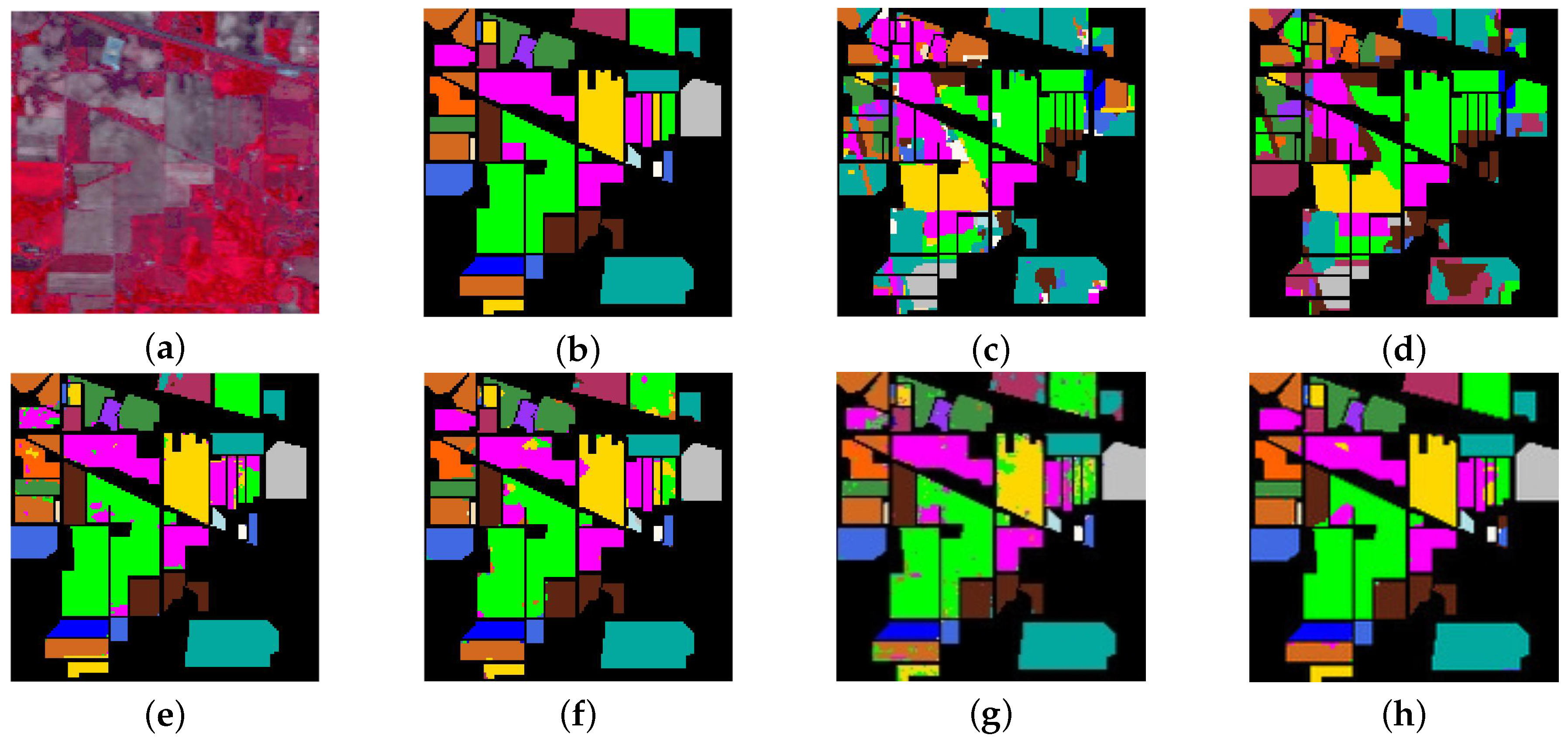
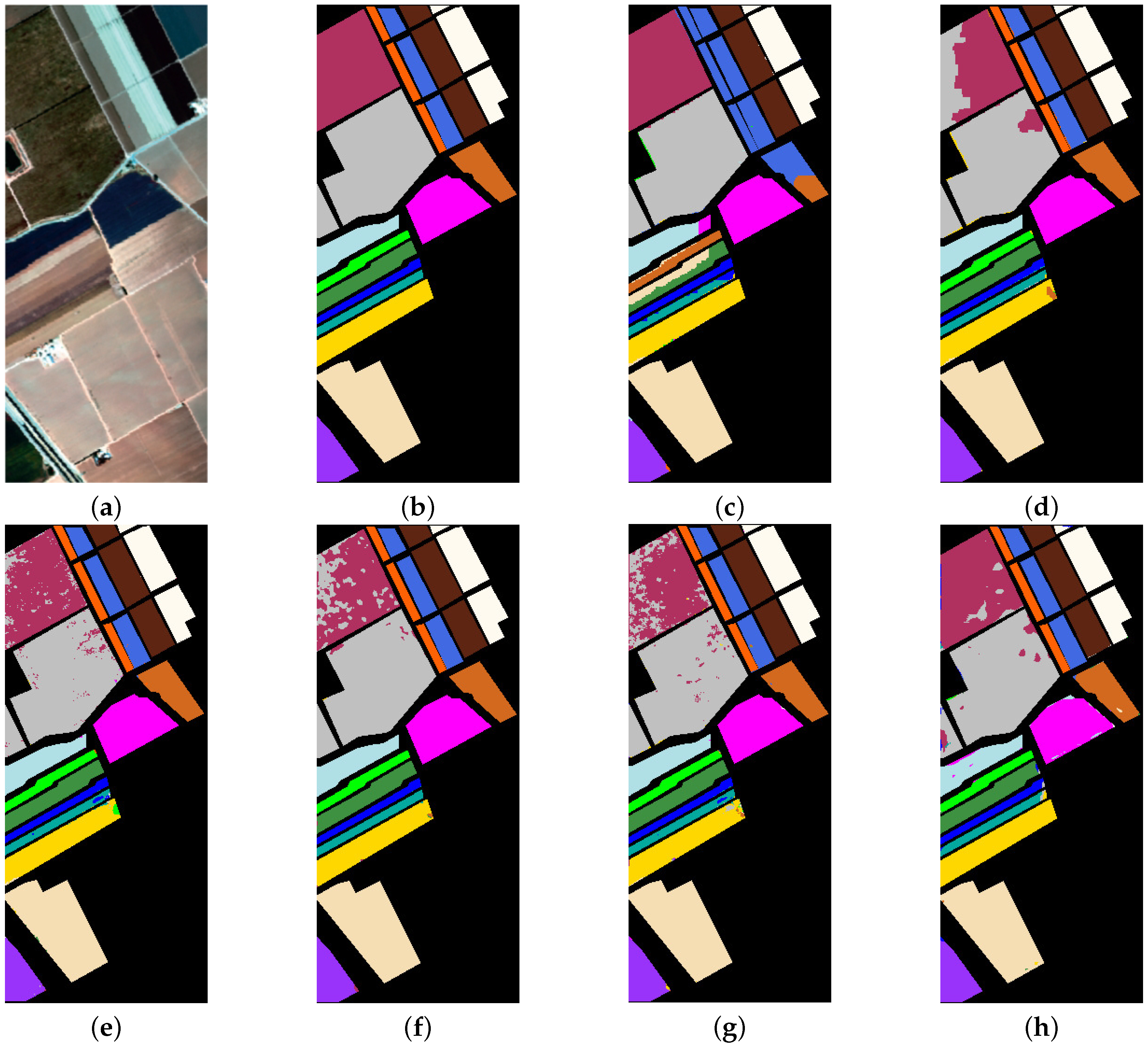
Next, we will show the advances of the proposed ASU-3D/2DNets compared to the state-of-the-art algorithms for HSI classification. Related results on Indian Pines, Salinas Valley, Kennedy Space Center (KSC), and Pavia University datasets are shown in Table 3, Table 4, Table 5 and Table 6, respectively. The corresponding classification maps are shown in Figure 10, Figure 11, Figure 12 and Figure 13. As can be seen from the tables, in all compared methods, our ASU-3D/2DNets achieves the best performance on four datasets, of which 96.34% on Indian Pines, 98.92% on Salinas Valley, 92.82% on KSC, and 98.64% on Pavia University. For deep learning-based methods, R-VCANet adopt advanced endmember-based convolution to explore the deep features in the HSI data; SSRN learns deep spectral-spatial features by decomposing 3D convolutions; MSDN-SA directly extends the 2D DenseNets architecture into 3D DenseNets; the ASU-3D/2DNets still performs the best. In addition, regarding subspace projection-based methods to separate mixed pixels (such as MLRsubMLL, SVM-MLRsub-MRF) with the best accuracy up to 87.82% on Indian Pines, 93.85% on Salinas Valley, 80.07% on KSC, and 93.85% on Pavia University, our proposed ASU-3D/2DNets performs the best.
4. Experimental Analysis
In this section, experiments on effect of training samples is shown firstly. Then, we qualitatively evaluate the performance of the early-exiting strategy in the proposed framework. Then, we investigate the efficacy of the adaptive spectral unmixing by confusion matrix obtained from the classification results. Then, we provide an ablation study of our ASU-3D/2DNets on four datasets. Lastly, experimental analysis on challenging HSI dataset is provided.
4.1. Effect of Training Samples
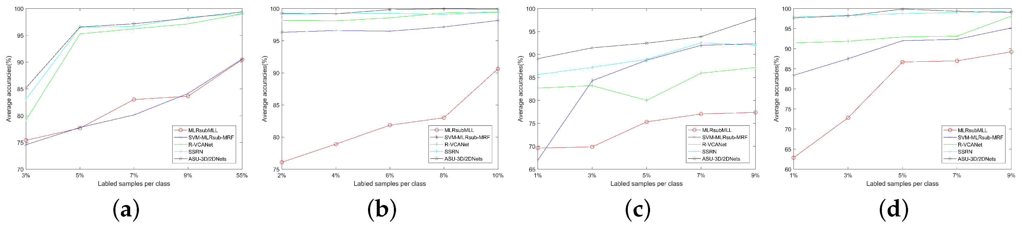
The above experimental results have shown that the proposed ASU-3D/2DNets method performs well in HSI classifications, especially in the case of having smaller training samples. In this part, we would like to further investigate the scenarios of extremely scarce training samples. The curves of AA, with respect to a different number of training samples, are shown in Figure 14.
As expected, as the number of training samples increases, the accuracy increases. We can see from Figure 14 that ASU-3D/2DNets outperforms other methods in most cases. Regarding Salinas Valley, KSC, and Pavia University datasets using only small training samples per class, ASU-3D/2DNets has achieved best. Although classification of Indian Pines dataset is more challenging, on 3–9% training samples per class, ASU-3D/2DNets scores significantly higher than other compared methods. It is worth mentioning that 55% of the training samples selected in the Indian dataset were allocated according to GRSS DASE website [42], and the algorithm also showed good classification results under fixed train/test data.
4.2. Analysis of Early-Exiting Strategy and Unmixing
In order to evaluate the performance of the early-exiting strategy in the proposed framework, quantitative data in the experiments are carried out on four datasets. As shown in Table 7, Table 8, Table 9 and Table 10, the first column indicates the block number, the second column indicates the output threshold of softmax for different blocks, the third column indicates the number and correct rate of sample output at T without unmixing, and the fourth column indicates that, under T, the number and correct rate of sample output at the time of unmixing. It should be noted that we set the to 0.75, following the practice in Reference [14]. In the early-exiting strategy, the number of samples output per block is changed by the correct rate before and after unmixing. According to the value of T, the classification result is outputted from the first two blocks successively, and the remaining samples are output in the last block, so the value of T in the last block is null.
Next, we investigate the efficacy of the adaptive spectral unmixing through confusion matrix obtained from the classification results. Under the early-exiting strategy of our proposed ASU-3D/2DNets, we remove the adaptive spectral unmixing method and represent this model as 3D/2DNets. Take KSC dataset as an example, the confusion matrix of the classification obtained by the 3D/2DNets and ASU-3D/2DNets is shown in Table 11 and Table 12, respectively. As shown in Table 11, from line five, we can see that confusion between CP/oak hammock and Slash pine (class 4 and class 5) is significant. After adding the adaptive spectral unmixing strategy as shown in Table 12, the number of samples in class 5 that were misclassified to the class 4 decreased from 48 to 9, reducing nearly 80%. In Table 11, for the Cattail marsh (class 10) of line ten, the misclassified samples are distributed in the Spartina marsh (class 9) and Mud flats (class 12). In Table 12, class 10 is completely separated from class 9. However, 3D/2DNets provides more accurate classification scores than ASU-3D/2DNets in class 8. In general, the performance of the 3D/2DNets becomes further improved by incorporating the adaptive spectral unmixing, with its OA increasing from 88.62% to 92.95% on KSC dataset. It can be inferred from the above analysis that spectral unmixing provides a useful source of information for classification and has the ability to further interpret mixed pixels, especially for classes where highly mixed pixels are dominant and its classification labels may be changed accordingly.
4.3. Ablation Study
To assess the performance gain caused by spectral-spatial 3D/2D convolution (SSDC), multiple intermediate classifiers, and adaptive spectral unmixing, we compared the proposed ASU-3D/2DNets with another four deep learning architectures. The first one, denoted by Model-B, is identical to the proposed one except for replacing each SSDC with a 3D convolutional kernel. The last two, denoted by Model-C and Model-D, are same with the proposed one except for either removing the adaptive spectral unmixing or removing the first two classifiers. To make a fair comparison, the same preprocessing strategy was used. The obtained OA, AA, values were displayed in Table 13, Table 14, Table 15 and Table 16. Take Indian Pines dataset as an example, where it shows that, compared to using 3D convolutional layers, using SSDC improves the OA from 0.9567 to 0.9634. It indicates that, compared with conventional 3D convolution, the SSDC can learn and represent spectral-spatial features more efficiently and accurately. Besides, either multiple intermediate classifiers or adaptive spectral unmixing can improve the performance to some extent. It is worth noting that the test samples passed through a deeper network layer in Model-D leads to no further improvement, but the model contained much more parameters and computational requirements. The same conclusion can be obtained by analyzing the other three datasets.
All these results show that the proposed ASU-3D/2DNets outperforms the state-of-the-art HSI classification methods. The design of the multiple intermediate classifiers make it possible to use adaptive spectral unmixing to facilitate classification, which brings considerable benefits for computational requirements and final performance. In addition, SSDC is more capable of processing spectral-spatial features than conventional 3D convolution, and each component of SSDC does help improve classification results.
4.4. Experimental Analysis on Challenging HSI Dataset
In this section, we will explore the classification results of our algorithm on more challenging high resolution HSI datasets. The HSI we used are provided by the Image Analysis and Data Fusion Technical Committee in the 2018 IEEE GRSS Data Fusion Contest, which are the images of the University of Houston Energy Research Park (UHEP) and the Earth and Atmospheric Science building (UH01) and one temporary station located at the Baytown airport (KHPY) [43]. It contains 48 bands with a spectral range of 380–1050 nm and a spatial resolution of 1 meter. The size of this data is , and it contains 50,4856 labeled reference samples. The classes and the number of labeled samples in each are listed in Table 17. Classification results of Houston 2018 dataset with different numbers of training samples are shown in Table 18.
It can be seen from Table 18 that our algorithm does not perform well in this dataset, and we analyze the reasons as follows.
Firstly, Table 17 shows the samples in the given hyperspectral image are severely unbalanced. Some classes, e.g., buildings and roads, have an adequate amount of data for training. However, classes, such as water, unpaved parking lots, and artificial turf, contain less than seven hundred samples. It has been well known that unbalanced training data may result in an underperformance of the network. Therefore, for this dataset, the future work of our algorithm needs to carry out a data augmentation method for the problem of unbalanced data, so as to re-balance the training data while keeping the data diversity.
Secondly, after adding the unmixing step, the classification result of the algorithm will not improve but decrease. We analyze that, since our algorithm is designed for the dataset with low resolution, and the spatial resolution of Houston 2018 is relatively high, further unmixing on preliminary classification results will have a bad effect on the classification result. Therefore, it can be concluded that our algorithm is more suitable for HSI with mixed pixels at low resolution.
5. Conclusions
In this paper, we proposed a network architecture specifically designed for low resolution hyperspectral datasets with mixed pixels. Based on the fact that HSI data is typically a mix of easy and hard examples, in this paper, we proposed a specially designed framework for HSI classification jointly using 3D/2D dense networks with multiple intermediate classifiers (i.e., 3D/2DNets) with an adaptive spectral unmixing. The design of the multiple intermediate classifiers with early-exiting strategy make it possible to use adaptive spectral unmixing to facilitate classification, which can decrease the computational requirements and improve final classification results. Besides, we proposed a 3D/2D convolution based on spectral-spatial information for the proposed framework, which fully takes advantage of 2D convolutions to obtain more spectral information, so that the 3D convolution can incorporate fewer 3D convolutions, while achieving feature learning, thereby reducing the training complexity of spectral-spatial fusion. Experimental results on four benchmark datasets show the proposed method outperforms state-of-the-art deep learning based and traditional HSI classification methods.
Author Contributions
All the authors made significant contributions to this work. B.F. devised the approach and analyzed the data; Y.L. helped design the experiments and provided advice for the preparation and revision of the work; B.F. performed the experiments; and Y.B. helped with the experiments. All authors have read and agreed to the published version of the manuscript.
Funding
The work was supported in part by the National Natural Science Foundation of China (61871460, 61876152) and Fundamental Research Funds for the Central Universities (3102019ghxm016).
Acknowledgments
The authors would like to thank P. Gamba from the Pavia University, Pavia, Italy, for providing the reflective optics system imaging spectrometer data and corresponding reference information.
Conflicts of Interest
The authors declare no competing financial interests. The founding sponsors had no role in the design of the study; in the collection, analyses, or interpretation of data; in the writing of the manuscript, and in the decision to publish the results.
References
- Bioucas-Dias, J.M.; Plaza, A.; Dobigeon, N.; Parente, M.; Du, Q.; Gader, P.; Chanussot, J. Hyperspectral unmixing overview: Geometrical, statistical, and sparse regression-based approaches. IEEE J. Sel. Topics Appl. Earth Observ. Remote Sens. 2012, 5, 354–379. [Google Scholar] [CrossRef] [Green Version]
- Dópido, I.G. New techniques for hyperspectral image classification. Ph.D. Thesis, Universidad de Extremadura, Extremadura, Spain, 2013. [Google Scholar]
- Fauvel, M.; Tarabalka, Y.; Benediktsson, J.A.; Chanussot, J.; Tilton, J.C. Advances in spectral-spatial classification of hyperspectral images. Proc. IEEE 2012, 101, 652–675. [Google Scholar] [CrossRef] [Green Version]
- Xu, S.; Li, J.; Khodadadzadeh, M.; Marinoni, A.; Gamba, P.; Li, B. Abundance-indicated subspace for hyperspectral classification with limited training samples. IEEE J. Sel. Topics Appl. Earth Observ. Remote Sens. 2019, 12, 1265–1278. [Google Scholar] [CrossRef]
- Keshava, N.; Mustard, J.F. Spectral unmixing. IEEE Signal Proc. Mag. 2002, 19, 44–57. [Google Scholar] [CrossRef]
- Plaza, A.; Benediktsson, J.A.; Boardman, J.W.; Brazile, J.; Bruzzone, L.; Camps-Valls, G.; Chanussot, J.; Fauvel, M.; Gamba, P.; Gualtieri, A.; et al. Recent advances in techniques for hyperspectral image processing. Remote Sens. Environ. 2009, 113, S110–S122. [Google Scholar] [CrossRef]
- Lanaras, C.; Baltsavias, E.; Schindler, K. Hyperspectral super-resolution by coupled spectral unmixing. In Proceedings of the IEEE International Conference on Computer Vision, Santiago, Chile, 7–13 December 2015; pp. 3586–3594. [Google Scholar]
- Yang, J.; Zhao, Y.Q.; Chan, J.C.W.; Kong, S.G. Coupled sparse denoising and unmixing with low-rank constraint for hyperspectral image. IEEE Trans. Geosci. Remote Sens. 2015, 54, 1818–1833. [Google Scholar] [CrossRef]
- Ertürk, A.; Plaza, A. Informative change detection by unmixing for hyperspectral images. IEEE Geosci. Remote Sens. Lett. 2015, 12, 1252–1256. [Google Scholar] [CrossRef]
- Dópido, I.; Zortea, M.; Villa, A.; Plaza, A.; Gamba, P. Unmixing prior to supervised classification of remotely sensed hyperspectral images. IEEE Geosci. Remote Sens. Lett. 2011, 8, 760–764. [Google Scholar] [CrossRef]
- Dópido, I.; Villa, A.; Plaza, A.; Gamba, P. A quantitative and comparative assessment of unmixing-based feature extraction techniques for hyperspectral image classification. IEEE J. Sel. Topics Appl. Earth Observ. Remote Sens. 2012, 5, 421–435. [Google Scholar] [CrossRef]
- Alam, F.I.; Zhou, J.; Tong, L.; Liew, A.W.C.; Gao, Y. Combining unmixing and deep feature learning for hyperspectral image classification. In Proceedings of the IEEE 2017 International Conference on Digital Image Computing: Techniques and Applications (DICTA), Sydney, NSW, Australia, 29 November–1 December 2017; pp. 1–8. [Google Scholar]
- Ibarrola-Ulzurrun, E.; Drumetz, L.; Marcello, J.; Gonzalo-Martín, C.; Chanussot, J. Hyperspectral classification through unmixing abundance maps addressing spectral variability. IEEE Trans. Geosci. Remote Sens. 2019, 57, 4775–4788. [Google Scholar] [CrossRef]
- Dópido, I.; Li, J.; Gamba, P.; Plaza, A. A new hybrid strategy combining semisupervised classification and unmixing of hyperspectral data. IEEE J. Sel. Topics Appl. Earth Observ. Remote Sens. 2014, 7, 3619–3629. [Google Scholar] [CrossRef]
- Li, J.; Dópido, I.; Gamba, P.; Plaza, A. Complementarity of discriminative classifiers and spectral unmixing techniques for the interpretation of hyperspectral images. IEEE Trans. Geosci. Remote Sens. 2014, 53, 2899–2912. [Google Scholar] [CrossRef]
- Sun, Y.; Zhang, X.; Plaza, A.; Li, J.; Dópido, I.; Liu, Y. A new semi-supervised classification strategy combining active learning and spectral unmixing of hyperspectral data. In High-Performance Computing in Geoscience and Remote Sensing VI; SPIE: Bellingham, WA, USA, 2016; Volume 10007, p. 1000708. [Google Scholar]
- Samat, A.; Li, J.; Liu, S.; Du, P.; Miao, Z.; Luo, J. Improved hyperspectral image classification by active learning using pre-designed mixed pixels. Pattern Recognit. 2016, 51, 43–58. [Google Scholar] [CrossRef]
- Pan, B.; Shi, Z.; Xu, X. R-VCANet: A new deep-learning-based hyperspectral image classification method. IEEE J. Sel. Topics Appl. Earth Observ. Remote Sens. 2017, 10, 1975–1986. [Google Scholar] [CrossRef]
- Chen, Y.; Jiang, H.; Li, C.; Jia, X.; Ghamisi, P. Deep feature extraction and classification of hyperspectral images based on convolutional neural networks. IEEE Trans. Geosci. Remote Sens. 2016, 54, 6232–6251. [Google Scholar] [CrossRef] [Green Version]
- Zhong, Z.; Li, J.; Luo, Z.; Chapman, M. Spectral–spatial residual network for hyperspectral image classification: A 3-D deep learning framework. IEEE Trans. Geosci. Remote Sens. 2017, 56, 847–858. [Google Scholar] [CrossRef]
- Fang, B.; Li, Y.; Zhang, H.; Chan, J.C.W. Hyperspectral images classification based on dense convolutional networks with spectral-wise attention mechanism. Remote Sens. 2019, 11, 159. [Google Scholar] [CrossRef] [Green Version]
- Fang, B.; Li, Y.; Zhang, H.; Chan, J.C.W. Collaborative learning of lightweight convolutional neural network and deep clustering for hyperspectral image semi-supervised classification with limited training samples. ISPRS J. Photogramm. Remote Sens. 2020, 161, 164–178. [Google Scholar] [CrossRef]
- Sutskever, I.; Hinton, G.E.; Krizhevsky, A. Imagenet classification with deep convolutional neural networks. In Proceedings of the 2012 Advances in Neural Information Processing Systems Conference, Stateline, NV, USA, 3–8 December 2012; pp. 1097–1105. [Google Scholar]
- He, K.; Zhang, X.; Ren, S.; Sun, J. Deep residual learning for image recognition. In Proceedings of the IEEE 2016 Conference on Computer Vision and Pattern Recognition, Las Vegas, NV, USA, 27–30 June 2016; pp. 770–778. [Google Scholar]
- Girshick, R.; Donahue, J.; Darrell, T.; Malik, J. Region-based convolutional networks for accurate object detection and segmentation. IEEE Trans. Pattern Anal. Mach. Intell. 2015, 38, 142–158. [Google Scholar] [CrossRef]
- Farabet, C.; Couprie, C.; Najman, L.; LeCun, Y. Learning hierarchical features for scene labeling. IEEE Trans. Pattern Anal. Mach. Intell. 2012, 35, 1915–1929. [Google Scholar] [CrossRef] [Green Version]
- Chan, T.H.; Jia, K.; Gao, S.; Lu, J.; Zeng, Z.; Ma, Y. PCANet: A simple deep learning baseline for image classification? IEEE Trans. Image Proc. 2015, 24, 5017–5032. [Google Scholar] [CrossRef] [PubMed] [Green Version]
- Paoletti, M.; Haut, J.; Plaza, J.; Plaza, A. Deep learning classifiers for hyperspectral imaging: A review. ISPRS J. Photogramm. Remote Sens. 2019, 158, 279–317. [Google Scholar] [CrossRef]
- Wang, W.; Dou, S.; Jiang, Z.; Sun, L. A fast dense spectral–spatial convolution network framework for hyperspectral images classification. Remote Sens. 2018, 10, 1068. [Google Scholar] [CrossRef] [Green Version]
- Paoletti, M.E.; Haut, J.M.; Plaza, J.; Plaza, A. Deep&dense convolutional neural network for hyperspectral image classification. Remote Sens. 2018, 10, 1454. [Google Scholar]
- Huang, G.; Liu, Z.; Van Der Maaten, L.; Weinberger, K.Q. Densely connected convolutional networks. In Proceedings of the 2017 IEEE Conference on Computer Vision and Pattern Recognition, Honolulu, HI, USA, 21–26 July 2017; pp. 4700–4708. [Google Scholar]
- Yu, F.; Koltun, V. Multi-scale context aggregation by dilated convolutions. arXiv 2015, arXiv:1511.07122. [Google Scholar]
- Köpüklü, O.; Kose, N.; Gunduz, A.; Rigoll, G. Resource efficient 3D convolutional neural networks. arXiv 2019, arXiv:1904.02422. [Google Scholar]
- Heinz, D.C. Fully constrained least squares linear spectral mixture analysis method for material quantification in hyperspectral imagery. IEEE Trans. Geosci. Remote Sens. 2001, 39, 529–545. [Google Scholar] [CrossRef] [Green Version]
- Huang, G.; Chen, D.; Li, T.; Wu, F.; van der Maaten, L.; Weinberger, K.Q. Multi-scale dense networks for resource efficient image classification. arXiv 2017, arXiv:1703.09844. [Google Scholar]
- Li, Y.; Zhang, H.; Shen, Q. Spectral–spatial classification of hyperspectral imagery with 3D convolutional neural network. Remote Sens. 2017, 9, 67. [Google Scholar] [CrossRef] [Green Version]
- Jiang, Y.; Li, Y.; Zhang, H. Hyperspectral image classification based on 3-D separable ResNet and transfer learning. IEEE Geosci. Remote Sens. Lett. 2019, 16, 1949–1953. [Google Scholar] [CrossRef]
- Zhou, Y.; Sun, X.; Zha, Z.J.; Zeng, W. Mict: Mixed 3d/2d convolutional tube for human action recognition. In Proceedings of the 2018 IEEE Conference on Computer Vision and Pattern Recognition, Salt Lake City, UT, USA, 18–22 June 2018; pp. 449–458. [Google Scholar]
- Tran, D.; Wang, H.; Torresani, L.; Ray, J.; LeCun, Y.; Paluri, M. A closer look at spatiotemporal convolutions for action recognition. In Proceedings of the 2018 IEEE Conference on Computer Vision and Pattern Recognition, Salt Lake City, UT, USA, 18–22 June 2018; pp. 6450–6459. [Google Scholar]
- Li, J.; Bioucas-Dias, J.M.; Plaza, A. Spectral–spatial hyperspectral image segmentation using subspace multinomial logistic regression and Markov random fields. IEEE Trans. Geosci. Remote Sens. 2011, 50, 809–823. [Google Scholar] [CrossRef]
- Khodadadzadeh, M.; Li, J.; Plaza, A.; Ghassemian, H.; Bioucas-Dias, J.M.; Li, X. Spectral–spatial classification of hyperspectral data using local and global probabilities for mixed pixel characterization. IEEE Trans. Geosci. Remote Sens. 2014, 52, 6298–6314. [Google Scholar] [CrossRef]
- GRSS DASE Website. Available online: http://dase.grss-ieee.org/ (accessed on 1 December 2019).
- 2018 IEEE GRSS Data Fusion Contest. Available online: http://www.grssieee.org/community/technical-committees/data-fusion (accessed on 1 December 2019).
Figure 1.
Illustration of the proposed framework adaptive spectral unmixing (ASU)-3D/2DNets.

Figure 2.
Illustration of dense networks with early-exiting strategy.

Figure 3.
Illustration of spectral-spatial 3D/2D convolution (SSDC).

Figure 4.
The classification results of each block in Indian Pines dataset.

Figure 5.
Reference map of the simulated hyperspectral dataset with four classes.

Figure 6.
Indian Pines image. (a) False color image. (b) Reference image.

Figure 7.
Salinas Valley image. (a) True color image. (b) Reference image.

Figure 8.
Kennedy Space Center (KSC) image. (a) True color image. (b) Reference image.

Figure 9.
Pavia University image. (a) True color image. (b) Reference image.

Figure 10.
Classification maps of Indian Pines dataset. (a) False color image. (b) Reference image. (c) MLRsubMLL. (d) SVM-MLRsub-MRF. (e) R-VCANet. (f) SSRN. (g) MSDN-SA. (h) ASU-3D/2DNets.
Figure 10.
Classification maps of Indian Pines dataset. (a) False color image. (b) Reference image. (c) MLRsubMLL. (d) SVM-MLRsub-MRF. (e) R-VCANet. (f) SSRN. (g) MSDN-SA. (h) ASU-3D/2DNets.

Figure 11.
Classification maps of Salinas Valley dataset. (a) True color image. (b) Reference image. (c) MLRsubMLL. (d) SVM-MLRsub-MRF. (e) R-VCANet. (f) SSRN. (g) MSDN-SA. (h) ASU-3D/2DNets.
Figure 11.
Classification maps of Salinas Valley dataset. (a) True color image. (b) Reference image. (c) MLRsubMLL. (d) SVM-MLRsub-MRF. (e) R-VCANet. (f) SSRN. (g) MSDN-SA. (h) ASU-3D/2DNets.

Figure 12.
Classification maps of KSC dataset. (a) True color image. (b) Reference image. (c) MLRsubMLL. (d) SVM-MLRsub-MRF. (e) R-VCANet. (f) SSRN. (g) MSDN-SA. (h) ASU-3D/2DNets.
Figure 12.
Classification maps of KSC dataset. (a) True color image. (b) Reference image. (c) MLRsubMLL. (d) SVM-MLRsub-MRF. (e) R-VCANet. (f) SSRN. (g) MSDN-SA. (h) ASU-3D/2DNets.

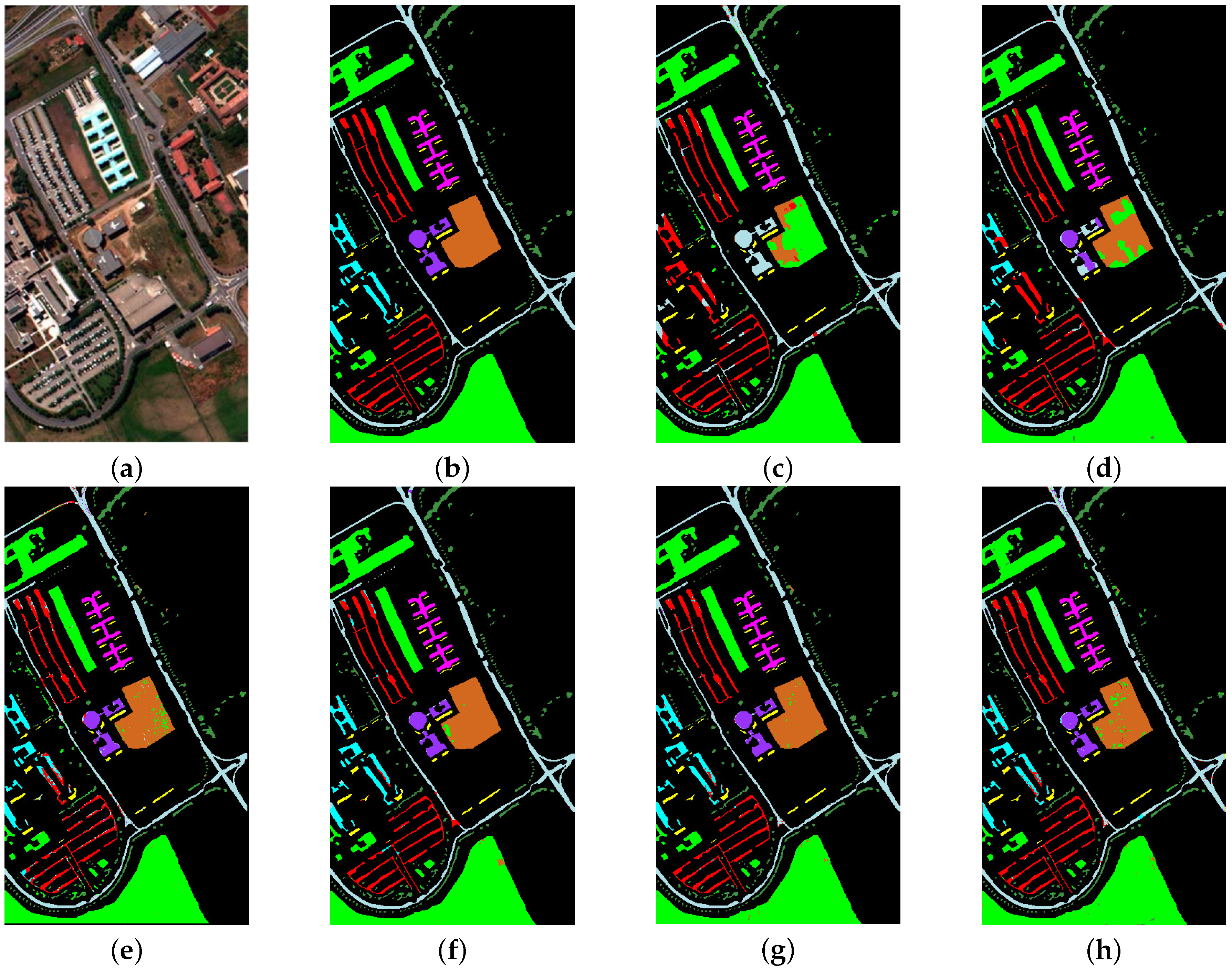
Figure 13.
Classification maps of Pavia University dataset. (a) True color image. (b) Reference image. (c) MLRsubMLL. (d) SVM-MLRsub-MRF. (e) R-VCANet. (f) SSRN. (g) MSDN-SA. (h) ASU-3D/2DNets.
Figure 13.
Classification maps of Pavia University dataset. (a) True color image. (b) Reference image. (c) MLRsubMLL. (d) SVM-MLRsub-MRF. (e) R-VCANet. (f) SSRN. (g) MSDN-SA. (h) ASU-3D/2DNets.

Figure 14.
Effect of number of training samples on: (a) Indian Pines dataset; (b) Salinas Valley dataset; (c) KSC dataset; and (d) Pavia University dataset.
Figure 14.
Effect of number of training samples on: (a) Indian Pines dataset; (b) Salinas Valley dataset; (c) KSC dataset; and (d) Pavia University dataset.


Table 1.
Network architecture details of proposed ASU-3D/2DNets.
| Type | |||
|---|---|---|---|
| Layer1 | Block1 | Block2 | Block3 |
| Avgpool3d | |||
Table 2.
Classification overall accuracy (%) of the synthetic dataset with different signal-to-noise-ratio (SNR). MLR = multinomial logistic regression; MLL = multilevel logistic; SVM = support vector machine; MRF = markov random field.
Table 2.
Classification overall accuracy (%) of the synthetic dataset with different signal-to-noise-ratio (SNR). MLR = multinomial logistic regression; MLL = multilevel logistic; SVM = support vector machine; MRF = markov random field.
| Algorithms | SNR | ||||||
|---|---|---|---|---|---|---|---|
| 20 | 25 | 30 | 35 | 40 | 45 | 50 | |
| MLRsubMLL | 85.97 ± 0.82 | 87.05 ± 0.83 | 88.99 ± 0.67 | 89.51 ± 0.55 | 90.36 ± 0.57 | 91.87 ± 0.21 | 92.42 ± 0.54 |
| SVM-MLRsub-MRF | 86.74 ± 0.74 | 88.48 ± 0.45 | 90.84 ± 0.34 | 91.97 ± 0.39 | 92.72 ± 0.48 | 93.48 ± 0.19 | 95.17 ± 0.23 |
| ASU-3D/2DNets | 90.15 ± 0.57 | 92.57 ± 0.18 | 94.28 ± 0.26 | 95.84 ± 0.24 | 95.97 ± 0.14 | 97.27 ± 0.21 | 98.96 ± 0.14 |
Table 3.
Classification results (%) of different algorithms on Indian Pines dataset with 5% training samples per class. OA = overall accuracy; AA = average accuracy; MSDN-SA = multiple scales dilated convolutions and a spectral-wise attention mechanism.
Table 3.
Classification results (%) of different algorithms on Indian Pines dataset with 5% training samples per class. OA = overall accuracy; AA = average accuracy; MSDN-SA = multiple scales dilated convolutions and a spectral-wise attention mechanism.
| Class | Samples | Methods | |||||
|---|---|---|---|---|---|---|---|
| No. | Training/ Validation /Testing | MLRsubMLL | SVM-MLRsub-MRF | R-VCANet | SSRN | MSDN-SA | ASU-3D/2DNets |
| 1 | 5/5/36 | 91.55 ± 4.48 | 31.11 ± 20.92 | 94.70 ± 5.12 | 100 ± 0 | 100 ± 0 | 100 ± 0 |
| 2 | 72/143/1213 | 74.47 ± 19.80 | 80.52 ± 3.99 | 91.12 ± 3.11 | 93.90 ± 2.17 | 94.65 ± 3.67 | 95.66 ± 2.83 |
| 3 | 42/83/705 | 81.04 ± 24.61 | 62.41 ± 8.67 | 93.46 ± 2.06 | 93.56 ± 4.82 | 92.80 ± 4.12 | 95.22 ± 3.03 |
| 4 | 12/24/201 | 35.71 ± 20.94 | 50.04 ± 34.87 | 92.07 ± 6.50 | 90.66 ± 8.18 | 91.87 ± 4.93 | 100 ± 0 |
| 5 | 25/49/409 | 57.42 ± 25.02 | 91.99 ± 2.65 | 96.99 ± 2.55 | 98.43 ± 1.04 | 97.89 ± 2.29 | 99.76 ± 0.21 |
| 6 | 37/73/620 | 95.75 ± 1.59 | 98.33 ± 1.29 | 99.98 ± 0.06 | 97.93 ± 2.64 | 97.88 ± 1.43 | 99.08 ± 0.65 |
| 7 | 2005/5/18 | 97.96 ± 3.75 | 64.29 ± 20.10 | 95.68 ± 1.51 | 99.24 ± 1.86 | 100 ± 0 | 95.45 ± 1.13 |
| 8 | 24/48/406 | 99.45 ± 0.12 | 99.53 ± 0.16 | 99.89 ± 0.18 | 98.67 ± 1.66 | 98.16 ± 2.41 | 95.73 ± 2.87 |
| 9 | 2005/5/10 | 100 ± 0 | 51.12 ± 48.38 | 85.96 ± 16.86 | 95.74 ± 4.99 | 88.24 ± 3.23 | 93.33 ± 1.98 |
| 10 | 49/98/825 | 39.00 ± 31.09 | 80.89 ± 5.29 | 93.73 ± 1.29 | 93.75 ± 5.33 | 86.72 ± 2.03 | 92.58 ± 3.74 |
| 11 | 123/246/2086 | 98.92 ± 0.96 | 97.85 ± 2.74 | 96.46 ± 1.77 | 97.08 ± 1.53 | 98.39 ± 1.62 | 95.25 ± 1.14 |
| 12 | 30/60/503 | 67.27 ± 31.89 | 93.95 ± 4.75 | 93.46 ± 3.16 | 93.97 ± 2.81 | 92.88 ± 1.87 | 97.25 ± 2.97 |
| 13 | 11/21/173 | 99.36 ± 0.24 | 98.43 ± 1.95 | 99.23 ± 0.84 | 99.29 ± 1.15 | 98.37 ± 0.62 | 97.34 ± 1.09 |
| 14 | 64/127/1074 | 100 ± 0 | 97.49 ± 2.14 | 99.60 ± 0.43 | 98.43 ± 1.12 | 98.53 ± 0.61 | 99.21 ± 0.27 |
| 15 | 20/39/327 | 12.34 ± 12.80 | 77.34 ± 21.21 | 92.59 ± 5.13 | 94.52 ± 5.39 | 95.92 ± 3.58 | 96.91 ± 3.21 |
| 16 | 5/10/78 | 92.70 ± 6.66 | 69.54 ± 37.18 | 99.43 ± 1.39 | 93.47 ± 6.85 | 90.43 ± 4.79 | 92.22 ± 3.04 |
| OA(%) | 79.87 ± 6.18 | 87.82 ± 2.37 | 95.68 ± 0.73 | 96.03 ± 0.58 | 95.47 ± 0.74 | 96.34 ± 1.40 | |
| AA(%) | 77.68 ± 4.67 | 77.80 ± 9.39 | 95.27 ± 0.91 | 96.50 ± 0.10 | 95.17 ± 0.89 | 96.56 ± 1.14 | |
| (%) | 76.47 ± 7.61 | 85.99 ±2.74 | 95.07 ± 0.83 | 95.29 ± 0.75 | 94.85 ± 0.81 | 95.83 ± 1.58 | |
Table 4.
Classification results (%) of different algorithms on Salinas Valley dataset with 2% training samples per class.
Table 4.
Classification results (%) of different algorithms on Salinas Valley dataset with 2% training samples per class.
| Class | Samples | Methods | |||||
|---|---|---|---|---|---|---|---|
| No. | Training/ Validation /Testing | MLRsubMLL | SVM-MLRsub-MRF | R-VCANet | SSRN | MSDN-SA | ASU-3D/2DNets |
| 1 | 41/201/1767 | 98.03 ± 3.80 | 100 ± 0 | 99.66 ± 0.18 | 100 ± 0 | 99.54 ± 0.77 | 100 ± 0 |
| 2 | 75/373/3278 | 99.94 ± 0.10 | 99.90 ± 0.11 | 99.86 ± 0.15 | 99.92 ± 0.10 | 99.97 ± 0.16 | 99.82 ± 0.41 |
| 3 | 40/198/1738 | 22.52 ± 17.78 | 99.38 ± 1.47 | 99.61 ± 0.26 | 99.66 ± 0.45 | 99.12 ± 1.37 | 100 ± 0 |
| 4 | 28/140/1226 | 13.99 ± 14.25 | 98.62 ± 1.50 | 98.59 ± 1.15 | 99.11 ± 0.91 | 98.68 ± 0.52 | 99.26 ± 0.48 |
| 5 | 54/268/2356 | 99.92 ± 0.01 | 98.76 ± 0.56 | 99.81 ± 0.24 | 99.93 ± 0.10 | 99.92 ± 0.04 | 99.87 ± 0.34 |
| 6 | 80/396/3483 | 99.93 ± 0.08 | 99.96 ± 0.06 | 99.97 ± 0.02 | 99.99 ± 0.01 | 99.95 ± 0.76 | 99.97 ± 0.29 |
| 7 | 72/358/3149 | 99.86 ± 0.04 | 99.65 ± 0.18 | 99.59 ± 0.50 | 99.93 ± 0.18 | 99.91 ± 0.24 | 100 ± 0 |
| 8 | 226/1128/9917 | 99.15 ± 0.20 | 96.20 ± 1.50 | 95.38 ± 0.96 | 95.26 ± 3.94 | 95.89 ± 5.18 | 97.22 ± 2.45 |
| 9 | 125/621/5457 | 100 ± 0 | 99.93 ± 0.14 | 99.81 ± 0.27 | 99.72 ± 0.28 | 99.93 ± 0.02 | 99.98 ± 0.19 |
| 10 | 66/328/2884 | 92.79 ± 3.96 | 95.54 ± 2.00 | 97.26 ± 0.98 | 99.59 ± 0.15 | 97.17 ± 2.83 | 99.48 ± 0.26 |
| 11 | 22/107/939 | 14.13 ± 34.62 | 95.19 ± 4.52 | 98.82 ± 0.76 | 99.43 ± 0.78 | 99.04 ± 0.19 | 98.54 ± 0.39 |
| 12 | 39/193/1695 | 56.19 ± 5.46 | 100 ± 0 | 100 ± 0 | 99.77 ± 0.44 | 100 ± 0 | 100 ± 0 |
| 13 | 19/92/805 | 99.41 ± 0.63 | 97.84 ± 0.91 | 99.10 ± 0.81 | 99.46 ± 1.27 | 99.89 ± 0.78 | 96.87 ± 3.67 |
| 14 | 22/107/941 | 91.03 ± 7.44 | 96.25 ± 1.54 | 93.79 ± 2.41 | 99.70 ± 0.37 | 94.71 ± 3.82 | 100 ± 0 |
| 15 | 146/727/6395 | 32.83 ± 50.86 | 65.19 ± 5.76 | 90.73 ± 1.67 | 94.02 ± 4.20 | 90.98 ± 6.04 | 97.49 ± 0.53 |
| 16 | 37/181/1589 | 97.74 ± 0.49 | 98.52 ± 0.75 | 98.65 ± 1.13 | 99.97 ± 0.08 | 97.83 ± 1.65 | 99.81 ± 0.46 |
| OA(%) | 81.35 ± 6.42 | 93.85 ± 0.90 | 97.30 ± 0.26 | 98.25 ± 0.51 | 97.47 ± 0.82 | 98.92 ± 0.42 | |
| AA(%) | 76.09 ± 3.41 | 96.31 ± 0.73 | 98.16 ± 0.26 | 99.15 ± 0.14 | 98.28 ± 0.76 | 99.27 ± 0.33 | |
| (%) | 78.97 ± 7.32 | 93.13 ± 1.01 | 96.99 ± 0.29 | 97.75 ± 0.89 | 97.18 ± 0.29 | 98.80 ± 0.46 | |
Table 5.
Classification results (%) of different algorithms on KSC dataset with 1% training samples per class.
Table 5.
Classification results (%) of different algorithms on KSC dataset with 1% training samples per class.
| Class | Samples | Methods | |||||
|---|---|---|---|---|---|---|---|
| No. | Training/ Validation /Testing | MLRsubMLL | SVM-MLRsub-MRF | R-VCANet | SSRN | MSDN-SA | ASU-3D/2DNets |
| 1 | 8//77/676 | 91.63 ± 2.03 | 100 ± 0 | 96.60 ± 2.37 | 96.34 ± 2.00 | 96.66 ± 1.53 | 95.26 ± 1.27 |
| 2 | 3/25/215 | 89.17 ± 10.19 | 59.58 ± 25.88 | 68.55 ± 18.28 | 93.84 ± 8.51 | 100 ± 0 | 93.78 ± 8.89 |
| 3 | 3/26/227 | 54.55 ± 33.61 | 79.64 ± 23.55 | 83.00 ± 17.59 | 76.74 ± 24.02 | 61.47 ± 27.78 | 90.51 ± 10.86 |
| 4 | 3/26/223 | 50.60 ± 12.23 | 71.02 ± 22.29 | 59.76 ± 12.76 | 65.34 ± 18.64 | 55.26 ± 13.76 | 52.61 ± 15.28 |
| 5 | 2/17/142 | 47.80 ± 25.96 | 17.44 ± 18.23 | 88.81 ± 9.89 | 51.46 ± 15.78 | 53.47 ± 8.01 | 91.37 ± 0.13 |
| 6 | 3/23/203 | 43.36 ± 27.19 | 16.00 ± 39.19 | 42.99 ± 2.78 | 83.37 ± 13.84 | 66.03 ± 11.69 | 54.97 ± 20.14 |
| 7 | 2/11/92 | 48.54 ± 20.38 | 14.21 ± 10.31 | 86.73 ± 29.14 | 80.46 ± 20.15 | 94.74 ± 1.57 | 95.83 ± 2.14 |
| 8 | 5/44/382 | 70.66 ± 22.14 | 78.76 ± 21.17 | 69.18 ± 19.97 | 89.94 ± 10.69 | 90.46 ± 2.96 | 89.29 ± 1.02 |
| 9 | 6/52/462 | 77.24 ± 1.35 | 97.89 ± 5.16 | 99.42 ± 0.67 | 86.53 ± 8.87 | 81.03 ± 6.19 | 99.61 ± 1.24 |
| 10 | 5/41/358 | 50.13 ± 16.58 | 53.42 ± 13.02 | 88.45 ± 20.05 | 98.27 ± 2.70 | 100 ± 0 | 99.00 ± 0.42 |
| 11 | 5/42/372 | 94.93 ± 2.98 | 91.06 ± 11.16 | 94.36 ± 3.94 | 96.52 ± 3.81 | 99.44 ± 0.49 | 99.48 ± 1.07 |
| 12 | 6/51/446 | 88.33 ± 7.61 | 92.39 ± 7.78 | 97.03 ± 3.07 | 94.19 ± 4.05 | 96.07 ± 1.22 | 96.39 ± 0.64 |
| 13 | 10/93/824 | 97.82 ± 3.73 | 99.11 ± 0.99 | 100 ± 0 | 100 ± 0 | 100 ± 0 | 100 ± 0 |
| OA(%) | 78.04 ± 5.32 | 80.07 ± 3.89 | 87.89 ± 5.42 | 88.78 ± 1.19 | 89.30 ± 2.63 | 92.82 ± 0.94 | |
| AA(%) | 69.60 ± 8.21 | 66.96 ± 6.04 | 82.68 ± 8.18 | 85.62 ± 0.85 | 84.20 ± 3.20 | 89.08 ± 1.83 | |
| (%) | 75.53 ± 6.77 | 77.62 ± 4.44 | 86.47 ± 6.07 | 87.50 ± 1.34 | 88.08 ± 2.92 | 93.09 ± 1.05 | |
Table 6.
Classification results (%) of different algorithms on Pavia University dataset with 1% training samples per class.
Table 6.
Classification results (%) of different algorithms on Pavia University dataset with 1% training samples per class.
| Class | Samples | Methods | |||||
|---|---|---|---|---|---|---|---|
| No. | Training/ Validation /Testing | MLRsubMLL | SVM-MLRsub-MRF | R-VCANet | SSRN | MSDN-SA | ASU-3D/2DNets |
| 1 | 67/664/5900 | 96.10 ± 3.98 | 98.79 ± 1.38 | 90.98 ± 3.24 | 99.10 ± 0.69 | 99.09 ± 0.78 | 98.01 ± 0.03 |
| 2 | 187/1865/16597 | 99.90 ± 0.05 | 99.81 ± 0.23 | 99.48 ± 0.28 | 99.03 ± 0.49 | 99.05 ± 0.07 | 99.56 ± 0.12 |
| 3 | 21/210/1868 | 7.62 ± 14.28 | 54.66 ± 11.14 | 82.20 ± 5.17 | 96.65 ± 4.27 | 96.77 ± 1.37 | 95.84 ± 0.49 |
| 4 | 31/307/2726 | 55.95 ± 14.39 | 89.51 ± 7.58 | 84.89 ± 0.89 | 99.82 ± 0.11 | 99.92 ± 0.52 | 97.07 ± 1.37 |
| 5 | 14/135/1196 | 99.80 ± 0.23 | 99.51 ± 0.23 | 99.89 ± 0.13 | 99.64 ± 0.76 | 98.09 ± 0.43 | 100 ± 0 |
| 6 | 51/503/4475 | 28.69 ± 4.59 | 85.96 ± 7.27 | 94.44 ± 0.63 | 99.07 ± 0.87 | 99.53 ± 1.41 | 98.55 ± 0.18 |
| 7 | 14/133/1183 | 19.01 ± 0.99 | 35.08 ± 12.62 | 89.43 ± 4.19 | 94.41 ± 10.94 | 72.28 ± 7.75 | 95.86 ± 0.04 |
| 8 | 37/369/3276 | 62.71 ± 33.98 | 90.14 ± 7.06 | 89.07 ± 3.56 | 91.49 ± 3.16 | 89.18 ± 2.39 | 97.50 ± 1.58 |
| 9 | 10/95/842 | 97.22 ± 2.31 | 96.91 ± 4.24 | 92.64 ± 1.5 | 99.94 ± 0.15 | 100 ± 0 | 99.41 ± 0.14 |
| OA(%) | 76.89 ± 3.62 | 92.15 ± 1.35 | 94.30 ± 0.38 | 98.11 ± 0.70 | 96.98 ± 0.32 | 98.64 ± 0.36 | |
| AA(%) | 62.89 ± 5.45 | 83.38 ± 4.28 | 91.45 ± 0.27 | 97.68 ± 1.51 | 94.88 ± 0.27 | 97.97 ± 0.43 | |
| (%) | 67.35 ± 5.39 | 87.89 ± 4.40 | 92.43 ± 0.49 | 97.49 ± 0.93 | 95.99 ± 0.39 | 98.20 ± 0.47 | |
Table 7.
Analysis of early-exiting strategy on Indian Pines dataset.
| Block | T | No Unmixing | Add Unmixing |
|---|---|---|---|
| 1 | 0.8658 | 1300/1302(0.999) | 1300/1302(0.999) |
| 2 | 0.6916 | 2033/2257(0.901) | 2114/2257(0.937) |
| 3 | ∼ | 2711/5125(0.529) | 4028/5125(0.786) |
Table 8.
Analysis of early-exiting strategy on Salinas Valley dataset.
| Block | T | No Unmixing | Add Unmixing |
|---|---|---|---|
| 1 | 0.8658 | 7142/7142(1) | 7142/7142(1) |
| 2 | 0.6916 | 12279/13333(0.921) | 13279/13333(0.996) |
| 3 | ∼ | 16449/27144(0.606) | 23208/27144(0.855) |
Table 9.
Analysis of early-exiting strategy on KSC dataset.
| Block | T | No Unmixing | Add Unmixing |
|---|---|---|---|
| 1 | 0.8658 | 696/693(1) | 693/693(1) |
| 2 | 0.6916 | 1183/1292(0.916) | 1188/1292(0.920) |
| 3 | ∼ | 1990/2637(0.755) | 2117/2637(0.803) |
Table 10.
Analysis of early-exiting strategy on Pavia University dataset.
| Block | T | No Unmixing | Add Unmixing |
|---|---|---|---|
| 1 | 0.8658 | 5700/5705(0.999) | 5700/5705(0.999) |
| 2 | 0.6916 | 10324/11030(0.936) | 10544/11030(0.958) |
| 3 | ∼ | 13969/21328(0.655) | 18235/21328(0.855) |
Table 11.
Confusion matrix of the classification obtained by the 3D/2DNets on KSC dataset.
| Class No. | 1 | 2 | 3 | 4 | 5 | 6 | 7 | 8 | 9 | 10 | 11 | 12 | 13 |
|---|---|---|---|---|---|---|---|---|---|---|---|---|---|
| 1 | 654 | 7 | 0 | 5 | 0 | 6 | 0 | 4 | 0 | 0 | 0 | 0 | 0 |
| 2 | 6 | 185 | 0 | 0 | 0 | 0 | 10 | 14 | 0 | 0 | 0 | 0 | 0 |
| 3 | 1 | 0 | 189 | 28 | 8 | 0 | 0 | 0 | 1 | 0 | 0 | 0 | 0 |
| 4 | 3 | 4 | 58 | 88 | 29 | 38 | 0 | 3 | 0 | 0 | 0 | 0 | 0 |
| 5 | 0 | 0 | 0 | 48 | 73 | 17 | 0 | 4 | 0 | 0 | 0 | 0 | 0 |
| 6 | 27 | 0 | 13 | 34 | 4 | 120 | 5 | 0 | 0 | 0 | 0 | 0 | 0 |
| 7 | 0 | 8 | 0 | 0 | 0 | 0 | 84 | 0 | 0 | 0 | 0 | 0 | 0 |
| 8 | 0 | 4 | 0 | 1 | 1 | 0 | 0 | 345 | 14 | 0 | 0 | 17 | 0 |
| 9 | 10 | 0 | 0 | 0 | 0 | 0 | 0 | 9 | 437 | 0 | 5 | 1 | 0 |
| 10 | 0 | 0 | 0 | 0 | 0 | 0 | 0 | 0 | 21 | 325 | 0 | 12 | 0 |
| 11 | 0 | 0 | 0 | 0 | 0 | 0 | 0 | 0 | 0 | 1 | 369 | 2 | 0 |
| 12 | 0 | 0 | 0 | 0 | 0 | 0 | 0 | 39 | 0 | 4 | 0 | 403 | 0 |
| 13 | 0 | 0 | 0 | 0 | 0 | 0 | 0 | 0 | 0 | 0 | 0 | 0 | 824 |
| OA = 88.62%, AA = 82.51%, = 87.32% | |||||||||||||
Table 12.
Confusion matrix of the classification obtained by the ASU-3D/2DNets on KSC dataset.
| Class No. | 1 | 2 | 3 | 4 | 5 | 6 | 7 | 8 | 9 | 10 | 11 | 12 | 13 |
|---|---|---|---|---|---|---|---|---|---|---|---|---|---|
| 1 | 652 | 0 | 0 | 0 | 6 | 0 | 0 | 10 | 8 | 0 | 0 | 0 | 0 |
| 2 | 1 | 206 | 0 | 0 | 0 | 0 | 8 | 0 | 0 | 0 | 0 | 0 | 0 |
| 3 | 0 | 0 | 218 | 1 | 0 | 1 | 0 | 0 | 7 | 0 | 0 | 0 | 0 |
| 4 | 1 | 3 | 57 | 109 | 10 | 37 | 0 | 2 | 1 | 0 | 0 | 3 | 0 |
| 5 | 3 | 0 | 0 | 9 | 130 | 0 | 0 | 4 | 0 | 0 | 0 | 0 | 0 |
| 6 | 28 | 3 | 26 | 5 | 0 | 141 | 0 | 0 | 0 | 0 | 0 | 0 | 0 |
| 7 | 0 | 8 | 0 | 0 | 0 | 1 | 83 | 0 | 0 | 0 | 0 | 0 | 0 |
| 8 | 0 | 0 | 0 | 1 | 0 | 0 | 0 | 311 | 57 | 0 | 0 | 13 | 0 |
| 9 | 0 | 0 | 0 | 0 | 0 | 0 | 0 | 0 | 461 | 0 | 1 | 0 | 0 |
| 10 | 0 | 0 | 0 | 0 | 0 | 0 | 0 | 0 | 0 | 350 | 0 | 8 | 0 |
| 11 | 0 | 0 | 0 | 0 | 0 | 0 | 0 | 0 | 0 | 1 | 369 | 2 | 0 |
| 12 | 0 | 0 | 0 | 0 | 0 | 0 | 0 | 0 | 0 | 3 | 0 | 442 | 1 |
| 13 | 0 | 0 | 0 | 0 | 0 | 0 | 0 | 0 | 0 | 0 | 0 | 0 | 824 |
| OA = 92.95%, AA = 89.67%, = 92.14% | |||||||||||||
Table 13.
Classification accuracy (%) of three different types’ networks on Indian Pines dataset.
| Proposed | Model-B | Model-C | Model-D | |
|---|---|---|---|---|
| OA | 96.34 | 95.67 | 94.3 | 94.21 |
| AA | 96.56 | 95.78 | 93.88 | 93.9 |
| 95.83 | 95.05 | 93.29 | 93.84 |
Table 14.
Classification accuracy (%) of three different types’ networks on Salinas Valley dataset.
| Proposed | Model-B | Model-C | Model-D | |
|---|---|---|---|---|
| OA | 98.92 | 96.64 | 93.53 | 93.47 |
| AA | 99.27 | 98.79 | 94.17 | 94.88 |
| 98.8 | 96.25 | 93.47 | 93.54 |
Table 15.
Classification accuracy (%) of three different types’ networks on KSC dataset.
| Proposed | Model-B | Model-C | Model-D | |
|---|---|---|---|---|
| OA | 92.82 | 90.29 | 88.69 | 87.14 |
| AA | 89.08 | 86.43 | 85.49 | 85.26 |
| 93.09 | 89.19 | 88.05 | 87.58 |
Table 16.
Classification accuracy (%) of three different types’ networks on Pavia University dataset.
Table 16.
Classification accuracy (%) of three different types’ networks on Pavia University dataset.
| Proposed | Model-B | Model-C | Model-D | |
|---|---|---|---|---|
| OA | 98.64 | 97.86 | 95.01 | 95.96 |
| AA | 97.97 | 98.13 | 94.48 | 93.14 |
| 98.2 | 97.15 | 95.99 | 94.87 |
Table 17.
Class information for Houston 2018 dataset.
| No | Class Name | Class Number |
|---|---|---|
| 1 | Healthy grass | 9799 |
| 2 | Stressed grass | 32502 |
| 3 | Artificial turf | 684 |
| 4 | Evergreen trees | 13595 |
| 5 | Deciduous trees | 5021 |
| 6 | Bare earth | 4516 |
| 7 | Water | 266 |
| 8 | Residential buildings | 39772 |
| 9 | Non-residential buildings | 223752 |
| 10 | Roads | 45866 |
| 11 | Sidewalks | 34029 |
| 12 | Crosswalks | 1518 |
| 13 | Major thoroughfares | 46348 |
| 14 | Highways | 9865 |
| 15 | Railways | 6937 |
| 16 | Paved parking lots | 11500 |
| 17 | Unpaved parking lots | 146 |
| 18 | Cars | 6547 |
| 19 | Trains | 5369 |
| 20 | Stadium seats | 6824 |
Table 18.
Classification results (%) of Houston 2018 dataset with different numbers of training samples.
Table 18.
Classification results (%) of Houston 2018 dataset with different numbers of training samples.
| The Proposed Algorithms | The Nnumber of Training Samples | ||
|---|---|---|---|
| 10% Per Class | 20% Per Class | 30% Per Class | |
| 3D/2DNets | 49.79 ± 5.88 | 62.53 ± 3.39 | 71.93 ± 2.98 |
| ASU-3D/2DNets | 46.30 ± 6.71 | 58.21 ± 4.18 | 70.56 ± 3.24 |
© 2020 by the authors. Licensee MDPI, Basel, Switzerland. This article is an open access article distributed under the terms and conditions of the Creative Commons Attribution (CC BY) license (http://creativecommons.org/licenses/by/4.0/).
Share and Cite
MDPI and ACS Style
Fang, B.; Bai, Y.; Li, Y. Combining Spectral Unmixing and 3D/2D Dense Networks with Early-Exiting Strategy for Hyperspectral Image Classification. Remote Sens. 2020, 12, 779. https://0-doi-org.brum.beds.ac.uk/10.3390/rs12050779
AMA Style
Fang B, Bai Y, Li Y. Combining Spectral Unmixing and 3D/2D Dense Networks with Early-Exiting Strategy for Hyperspectral Image Classification. Remote Sensing. 2020; 12(5):779. https://0-doi-org.brum.beds.ac.uk/10.3390/rs12050779
Chicago/Turabian StyleFang, Bei, Yunpeng Bai, and Ying Li. 2020. "Combining Spectral Unmixing and 3D/2D Dense Networks with Early-Exiting Strategy for Hyperspectral Image Classification" Remote Sensing 12, no. 5: 779. https://0-doi-org.brum.beds.ac.uk/10.3390/rs12050779
Note that from the first issue of 2016, this journal uses article numbers instead of page numbers. See further details here.