A Multi-Decadal Investigation of Tidal Creek Wetland Changes, Water Level Rise, and Ghost Forests


Department of Earth and Ocean Sciences, University of North Carolina Wilmington, 601 S. College Rd, Wilmington, NC 28403, USA
*
Author to whom correspondence should be addressed.
Remote Sens. 2020, 12(7), 1141; https://0-doi-org.brum.beds.ac.uk/10.3390/rs12071141
Submission received: 5 March 2020
/
Revised: 27 March 2020
/
Accepted: 31 March 2020
/
Published: 3 April 2020
(This article belongs to the Special Issue Remote Sensing of Coastal Processes)
Abstract
:Coastal wetlands play a vital role in protecting coastlines, which makes the loss of forested and emergent wetlands devastating for vulnerable coastal communities. Tidal creeks are relatively small hydrologic areas that feed into larger estuaries, are on the front lines of the interface between saltwater and freshwater ecosystems, and are potentially the first areas to experience changes in sea level. The goal of this study was to investigate wetland changes through time at two tidal creeks (Smith Creek and Town Creek) of the Cape Fear River estuary in southeastern North Carolina, USA, to determine if there is a spatial relationship between habitat change, physical geography characteristics, and the rate of wetland migration upstream. Historic aerial photography and recent satellite imagery were used to map land cover and compute change through time and were compared with derived physical geography metrics (sinuosity, creek width, floodplain width, floodplain elevation, and creek slope). The primary results were: (1) there was a net gain in emergent wetlands even accounting for the area of wetlands that became water, (2) wetlands have migrated upstream at an increasing rate through time, (3) land cover change was significantly different between the two creeks (P = 0.01) where 14% (67.5 ha) of Smith Creek and 18% (272.3 ha) of Town Creek transitioned from forest to emergent wetland, and (4) the transition from emergent wetland to water was significantly related to average change in creek width, floodplain elevation, and average water level. In conclusion, this research correlated habitat change with rising water level and identified similarities and differences between neighboring tidal creeks. Future research could apply the methodologies developed here to other coastal locations to further explore the relationships between tides, sea level, land cover change, and physical geography characteristics.

1. Introduction
There are several factors that influence wetland species presence and the transition/loss of wetlands through time. The primary driving factors that influence coastal wetlands are land cover change, sedimentation, relative sea-level rise (RSLR), tidal regime, topography, and location of the salt wedge [1]. Sediment accumulates naturally on wetlands from tidal inflow and runoff from upland areas. Under natural conditions, coastal wetlands accrete sediment from these sources and transgress inland at the same rate as RSLR [1]. If RSLR surpasses the rate at which coastal wetlands accumulate sediment, wetlands will transition to intertidal mudflats or open water [2,3,4]. Additionally, the salt wedge dictates the freshwater/saltwater boundary while the tidal range, ground elevation, and topography influence the duration and extent of tidal inundation and salinity. Specifically, low relief coastal areas experience vegetation changes with slight changes to the tidal range while this change is not as expansive in high relief locations.
Wetlands are also threatened by many natural and anthropogenic factors such as human modification along the coast, faster rates of RSLR, invasive non-native species, and tropical storms and hurricanes [5,6]. Wetlands are particularly vulnerable to increased rates of RSLR because as sea levels rise, tides and the saltwater wedge are pushed further upstream, resulting in freshwater tidal areas becoming brackish and non-tidal wetlands becoming tidally influenced. This push of tides brings saltier water further upstream and since freshwater forested and non-forested wetlands are not adapted to increased salinities, freshwater wetlands will transition to saltmarsh [7]. This transition results in “ghost forests” where dead trees remain standing in the herbaceous understory for years and provide evidence of historical forests [8,9,10].
Global mean sea-level rise was 1.7 mm/yr during the 20th century [11] and estimates for 2100, based on the Representative Concentration Pathways 8.5 scenario (which are based on a continued rise in greenhouse gas emissions throughout the 21st century) indicate global mean sea level will rise 0.52–0.98 m [12]. Alternatively, National Oceanic and Atmospheric Administration (NOAA) estimates of sea level rise takes into account Antarctic ice melt predicting a rise of 0.3–2.5 m and varies geographically [13]. In Wilmington, North Carolina, USA, the RSLR has been calculated to be 2.47 mm/yr [14].
1.1. Study Area
Located along the mid-Atlantic coast of the United States, the Cape Fear River estuary has a semi-diurnal, microtidal regime with a mean daily tidal range of 1.4 m at the Atlantic Ocean (Bald Head Island station 8658163) and 1.3 m tidal range 46 km upstream at the NOAA tide gauge located on Eagle Island, Wilmington, North Carolina (station 8658120) (Figure 1) [5,14,15]. The potential tidal influence extends further upstream to the United States Geological Survey (USGS) gauging station (station 02105769) at Lock and Dam No. 1, but water level is predominantly influenced by precipitation and river discharge [16]. Therefore, the extent to which rising tides versus seasonal changes in river discharge are related to water level is not well known in this study area. Further, the Cape Fear River shipping channel has been widened and deepened numerous times to allow larger ships to enter the Wilmington Port. Earliest records recorded a depth of 3.7 m in 1871 and dredging has increased the channel depth to 12.8 m at Mean Lower Low Water (MLLW) [17,18]. Dredging mimics the effects of increasing sea level, pushing tides and salinity further upstream, and has contributed a 0.26 m increase in tidal range in downtown Wilmington from 1889–1984 [19].
Previous research identified wetland transitions at isolated locations along the Cape Fear River, Northeast Cape Fear River, and two tidal creeks (Town Creek and Mott Creek) (Figure 1) [19,20]. From 1949–1978, bald cypress (Taxodium distichum) transitioned to brackish marsh species including black needlerush (Juncus roemerianus) and chairmaker’s bulrush (Scirpus olneyi) in Mott Creek [19]. Twelve sites were also studied from 2000–2009 and four of these experienced vegetation changes: (1) freshwater emergent vegetation transitioned to saltwater emergent vegetation, (2) forested wetlands transitioned to herbaceous, and (3) bald cypress showed salt stress [20].
Within the Cape Fear River estuary, wetland composition changes from the mouth of the river to the upstream tidal extent (Figure 2). At the mouth of the estuary (salinity >30 parts per thousand (ppt)), there is a limited number of species adapted to the high salinity and long inundation period, resulting in one dominant species, Sporobolus alternifolius (previously named Spartina alterniflora) in the low marsh and greater species diversity in the middle to high marsh (i.e., Juncus roemerianus, Distichlis spicata, and Salicornia virginica) [1,5]. Moving upstream, salinity decreases (30 to 0.5 ppt) and species diversity increases to a mixture of saltwater and freshwater species. Further up the estuary are tidal freshwater (<0.5 ppt) wetlands that are either forested or non-forested. Tidal freshwater non-forested wetlands are not characterized by species zonation and usually have a high species diversity consisting of annuals, perennials, broad-leafed trees, grasses, rushes, sedges, and herbaceous plants [15,20,21,22,23], while tidal freshwater forested wetlands are dominated by bald cypress (Taxodium distichum) [20,21]. Located furthest upstream, beyond the influence of tides, are non-tidal/riverine wetlands.
The coastal counties surrounding the Cape Fear River have experienced a large increase in urban population where, from 1970 to 2010, New Hanover County experienced a 144% increase in population and Brunswick County a 343% increase [24]. With population growth, and the potential loss of natural areas including forested wetlands, there is an increased coastal vulnerability to storm surge inundation and pluvial flooding. To investigate land cover change under increasing tidal range, relative sea-level rise, and urban development, two tidal creeks of the Cape Fear River estuary, Smith Creek (34.257029, -77.929373) and Town Creek (34.135822, -78.001620) were investigated in this study (Figure 1). Town Creek, 33 km from the mouth of the Cape Fear River, is characterized by expansive wetlands, and is very long for a tidal creek at 53 km [25]. Further upstream, 18 km from Town Creek, is Smith Creek which is much shorter in length (17 km) and is surrounded by urban development. While Smith Creek and Town Creek have notable differences, these creeks were chosen because: (1) they are in close proximity, which is good for comparison purposes; (2) field work could be accomplished over the same time frame; and (3) other studies have conducted some short-term salinity and vegetation analysis on these creeks (Figure 1) [20,26], but they were not spatially inclusive and did not cover a long time frame.
Each creek was divided into segments (lower, middle, and upper for Smith Creek and lower, lower-mid, upper-mid, and upper for Town Creek) in order to make comparisons between locations from downstream to upstream (Figure 1). The segment boundaries were based on a combination of anthropogenic influences (e.g., roads, power lines, railroads that crossed the creek) and size of the segment so that each creek had roughly the same size/area for each segment with exceptions when a road crossed the study area and this was a useful boundary.
1.2. Project Significance and Research Questions
Given that wetlands will transition from freshwater to saltwater under rising sea levels, and previous work in the Cape Fear River has documented isolated cases of wetland transitions [19,20], the goal for this project was to investigate wetland changes that address these research questions:
- Can airborne (historic aerial photography) and satellite imagery be used to identify where freshwater forested wetlands have changed to saltmarsh?
- Can aerial photography and satellite imagery be used to document salinity movement upstream?
- Have changes in wetland distributions been the same across multiple creeks?
- Is there a spatial relationship with the physical geography of creeks?
2. Materials and Methods
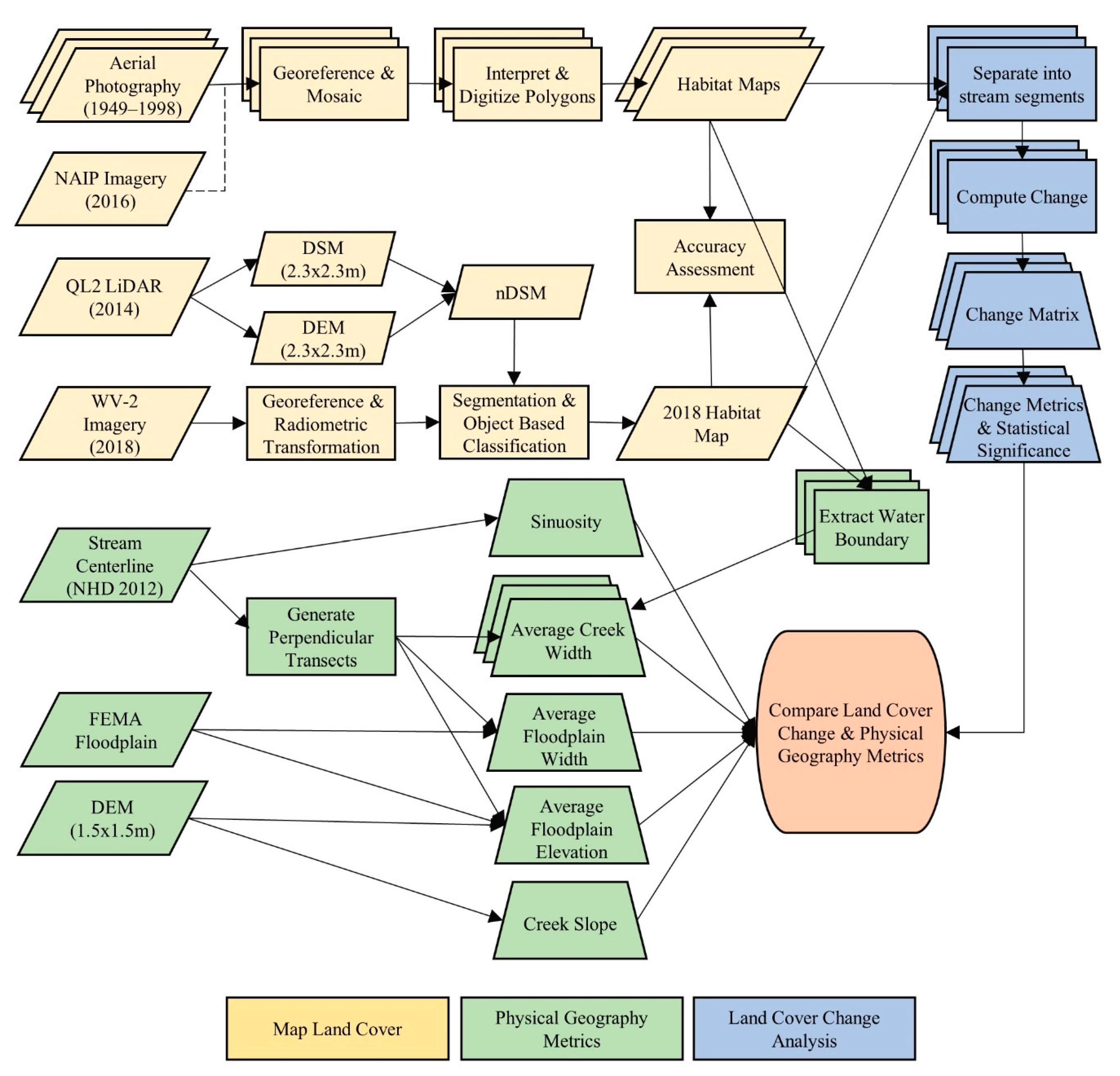
To address the research questions, methods consisted of field work, derivation of physical geography characteristics, mapping land cover, computing land cover change through time, and comparing the two study areas to identify similarities and differences. Specifically we conducted the following: (1) field work to gather ground reference data; (2) quantified water level with respect to semi-diurnal tides and compared with the nearest NOAA gauge; (3) computed physical geography metrics including sinuosity, creek width, floodplain width, floodplain elevation, and creek slope; (4) interpreted aerial photography from 1949 to 1998 and analyzed satellite imagery from 2018; and (5) assessed habitat changes through time with physical geography metrics (Figure 3).
2.1. Gather Ground Reference Data
Field work was conducted to gather Global Positioning System (GPS) coordinates and habitat types, install pressure transducers to measure water level, and install gauges to measure salinity (locations are shown in Figure 1). Gathering water level data was important in order to document how far tides extend up-creek and to measure the time differences between the creeks and the NOAA gauge. Five HOBO U20 Water Level Logger pressure transducers [29] were installed and recorded measurements every six minutes from 10 August 2018 to 9 September 2018. Three devices were installed in Smith Creek and only one device was placed in Town Creek because of extremely limited access to the creek. At Town Creek, one device was located on an upland site adjacent to the creek in order to convert barometric pressure to water level. We used HOBOware Pro 3.7.13 Barometric Pressure Assistant [30] to convert the barometric pressure data from the four devices to water level. Additionally, we used water temperature to account for fluid density to more accurately convert pressure to water level [31]. Tidal lag was calculated by measuring the time difference between consecutive high tides at the pressure transducers and the NOAA tide gauge in downtown Wilmington.
To measure salinity, three HOBO U24-002-C Salinity Data Loggers [32], two on Smith Creek and one on Town Creek, were installed and recorded every six minutes from 10 August 2018 to 9 September 2018 (locations are shown in Figure 1). Upon retrieval, conductivity was converted to salinity using HOBOware Pro 3.7.13 Conductivity Assistant [30] using a salt water for temperature compensation where water temperature was obtained from the pressure transducers [33].
2.2. Compute Physical Geography Metrics
To identify if there was a change in tidal range over time, daily water levels were obtained from 1936–2018 for the NOAA gauge located on Eagle Island [14] and tidal range was calculated based on the differences between high tide and low tide. To understand the characteristics of the two tidal creeks, we computed several physical geography metrics: sinuosity, creek width through time, floodplain width, floodplain elevation, and upstream to downstream creek slope (Supplementary Figures S1 and S2). These metrics were compared with the change in land cover to identify patterns in the study areas.
Sinuosity (S) describes the curviness of a line (Equation (1)):
where LS is stream length and LE is Euclidean distance.
S = LS/LE
A higher sinuosity corresponds to a creek that meanders more. The stream channel was defined using stream centerlines from the 2012 National Hydrography Dataset [34]. For each creek segment, a straight line was digitized to calculate the Euclidean distance which was compared with the length of the creek centerline.
To calculate floodplain width, transects were generated at 100 m intervals perpendicular to the Euclidean distance and then clipped to the Federal Emergency Management Agency (FEMA) 100-yr floodplain boundary [35]. To calculate the average elevation within the floodplain, a Digital Elevation Model (DEM) with 5x5 ft cell size was obtained from the North Carolina Department of Emergency Management [36] and then clipped to FEMA’s 100-yr floodplain boundary [35]. To calculate creek width, transects were generated perpendicular to the creek centerline and then clipped to the water extent. Creek width change through time was calculated using multiple dates of imagery (see dates and detailed imagery information provided below in Table 1, Section 2.3).
To calculate the slope of each creek, we identified the upper headwater location, buffered this point using a 50 m radius, and computed the average elevation. Similarly, we identified the mouth of the creek, buffered it 50 m, and computed the average elevation. Next, the slope between the headwater and mouth was the change in elevation divided by the length of the creek.
The forest/emergent wetland boundary indicates the upper extent of salinity due to the sensitivity of forested wetlands to salt, where exposure to >1 ppt for more than 25% of the time can initiate a change in vegetation [20]. Therefore, to determine if saltwater moved upstream through time, the location of the boundary between forest and emergent wetland was identified in each date of imagery. To determine if the rate of migration upstream was influenced by relative sea-level rise, or other factors, a tidal extension formula (Equation (2)) was created using information provided in previous research [37]:
where E is the rate of tidal extension (meters per year), R is the rate of relative sea-level rise, and S is the slope of the creek.
E = R/S
2.3. Map Land Cover
A variety of image sources (aerial photography and satellite imagery) with differing spatial and spectral characteristics were used to map land cover since the mid-1900s (Table 1) [38,39,40]. Aerial photography was used in this study in order to get a long time frame, which was important to capture when land cover transitions occurred, and historic aerial photography was useful for documenting habitat change in coastal environments [7,19,41,42]. WorldView-2 (WV-2) satellite imagery was used to map land cover due to the high spatial and spectral resolutions relative to other commercial satellites, and its success in mapping coastal habitats [43,44,45,46,47]. Due to the inherent differences between the aerial photography and satellite imagery, we used a variety of methods to map land cover (Figure 3).
Aerial photography was rectified in ArcMap 10.5.1 to 2016 National Agriculture Imagery Program (NAIP) orthorectified aerial photography (using Universal Transverse Mercator (UTM) coordinate system, North American Datum (NAD) 83, and cell size 2 m) [48]. A minimum of 50 ground reference points per image were used to perform rectification. We tested several approaches to deriving land cover through automated techniques, such as unsupervised, supervised, and object-based classifications, but none were successful with black-and-white aerial photography. Others have successfully used automated methods using natural color [49] and multispectral aerial photography [50,51], but black-and-white photography does not have the spectral information needed for successful automated mapping of coastal habitats [7,42,52]. Therefore, for each year, images were mosaicked and land cover polygons were digitized using a map scale of 1:1,000. Digitized polygons were classified into six categories: water, emergent wetland, forest, upland grass, developed, and bare ground. Black-and-white aerial photography was interpreted using textural differences while color infrared photographs were primarily interpreted using the vegetation response in the near-infrared band. Unfortunately, it was impossible to distinguish upland forest from freshwater forested wetland in the black-and-white imagery; therefore, both were grouped into a forest category. After digitization and classification, numerous topological error checks were conducted to ensure there were no gaps or overlapping features in the data.
To assess digitizing accuracy, 1 randomly selected polygon for each land cover type, for each year, was redigitized. This resulted in between 8% and 24% of the study area being redigitized for each year. Next, points were generated every 25 m along the new digitized land cover boundary and the distance from the new points to the original digitized polygon boundary was computed (Supplementary Figure S3). Spatial error was assessed by computing the positional uncertainty (Equation (3)) [49,50,51,52]:
where UT is the total positional uncertainty, D is the digitization error, and R is the rectification error.
WV-2 imagery collected on 19 July 2018 was used to generate the most recent land cover map of each study area. The imagery had 8 spectral bands with 2.29x2.29 m spatial resolution and 16-bit radiometric resolution [53]. Each image was preprocessed to convert digital numbers to surface reflectance by first radiometrically calibrating to absolute radiance, then ENVI’s fast line-of-sight atmospheric analysis of spectral hypercubes (FLAASH) was used to remove atmospheric scattering and absorption effect [54] and then the images were mosaicked together. To assist with image classification, 2014 QL2 Light Detection and Ranging (Lidar) data [36] were used to generate a DEM, Digital Surface Model (DSM), and Normalized Digital Surface Model (nDSM). Bare Earth returns were used to generate the DEM while the first returns were used to create the DSM. The nDSM was calculated as: DSM – DEM.
Image classification was performed using eCognition [55], an image segmentation and object-oriented classification software. eCognition has been successfully used to map wetland habitats [56,57] and, unlike per pixel classification methods, the object-oriented approach uses spectral and spatial parameters to define objects. Using the 2018 WV-2 imagery and 2014 Lidar terrain layers, the multi-resolution segmentation algorithm (scale, 75; shape, 0.1, compactness, 0.5) was used to merge neighboring pixels into objects based on their relative homogeneity. The objects were then classified into the six land cover classes (water, emergent wetland, forest, upland grass, developed, and bare ground) using a defined rule set. The specific values used in the rule set were determined from trial and error using several band indices and threshold values. The rule set incorporated the 8 bands from the WV-2, a Normalized Difference Bare Soil Index (NDBSI) (Equation (4)), two Normalized Difference Vegetation Indices (NDVI) (Equations (5) and (6)) [58], and the Lidar derived DEM and nDSM.
NDBSI = (Blue − Coastal)/(Blue + Coastal)
NDVI1 = (NIR1 − Red)/(NIR1 + Red)
NDVI2 = (Red − NIR2)/(Red + NIR2)
Lastly, a classification accuracy assessment using 30 randomly located points per land cover type with a minimum distance of 10 m between points for Smith Creek and 20 m between points for Town Creek was conducted on the final WV-2 map classifications.
2.4. Multi-Temporal Change Analysis
Five transition periods were analyzed for Smith Creek (1949–1956, 1656–1966, 1966–1980, 1980–1998, and 1998–2018) and three for Town Creek (1964–1980, 1980–1998, 1998–2018). For each transition period, change matrices were created for the entire creek and each creek segment. The transitions were analyzed by gain, loss, total change (sum of gains and losses), net change (difference between gains and losses), and swap change (total change minus the absolute value of the net change). Classification change matrices are useful for quantifying change; however, they do not identify transitions that changed more or less than expected [59]. To determine the transitions that changed more than expected, we calculated the expected gain (G, Equation (7)) and expected loss (L, Equation (8)) between land cover types based on the observed percentages of each land cover in time 1. We then tested the amount of change (deviation) by computing the difference between observed and expected change (C, Equation (9)). A high value of the deviation/expected ratio represents a greater amount of change than expected [59]. When the ratio of deviation/expected was greater than 1 standard deviation, the change between land cover types was considered significant.
where GB is the expected gain in class B, OB is the observed gain in class B, TA is the observed total of class A during the first time, and TB is the observed total of class B during the first time.
where LA is the expected loss of class A, OA is the observed loss of class A, TB is the observed total of class B during the second time, and TA is the observed total of class A during the second time.
where C is the amount of change, O is the observed change (gain or loss) between land cover types, and E is the expected change (gain or loss) between land cover types.
GB = OB (TA/(100 − TB))
LA = OA (TB/(100 − TA))
C = (O − E)/(E)
3. Results
3.1. Tides and Salinity
Since the installation of the NOAA tide gauge in 1936, the average tidal range has increased 0.41 m, the average high tide has increased 0.4 m, and average low tide has decreased 0.01 m. However, not all of the change in tidal range can be attributed to relative sea-level rise since the rate was 2.47 mm/yr [14] for a total of 0.202 m.
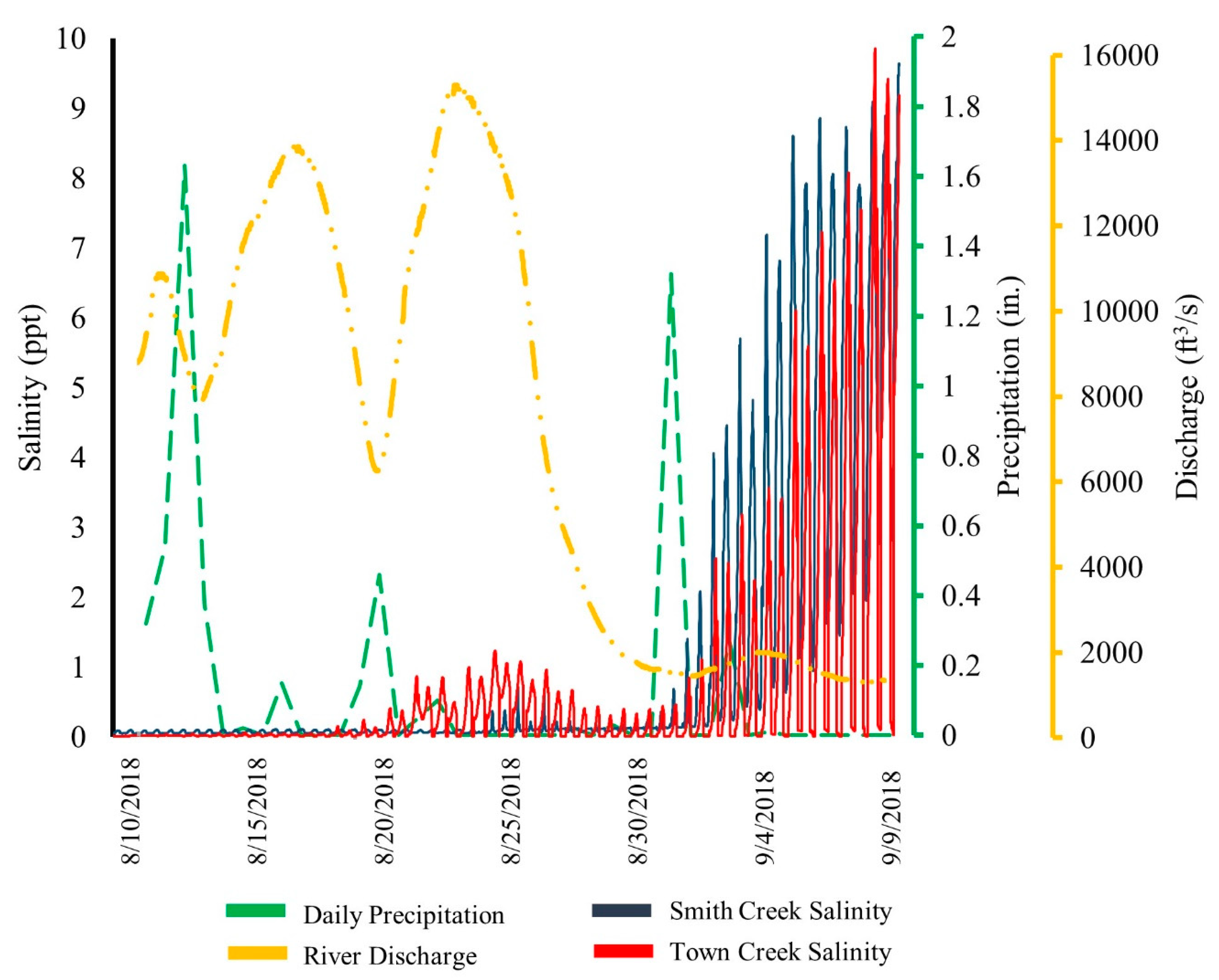
We compared the control pressure transducer, located adjacent to the creek shoreline, with the nearest airport, and there was no significant difference in barometric pressure. Therefore, we proceeded with the conversion to water level, which resulted in 62 high tides that were then compared with the NOAA tide gauge in downtown Wilmington. The time delay was 110 min for Town Creek and 38 min near the mouth of Smith Creek and 94 min in the upper reach of Smith Creek (see Supplementary Table S1 for detailed results). From 10 August 2018 to 9 September 2018, salinity ranged from 0.5–9.64 ppt at Smith Creek and 0.01–9.86 ppt at Town Creek.
3.2. Physical Geography Characteristics: Sinuosity, Elevation, Width, and Slope
Overall, sinuosity and floodplain width were greater at Town Creek than Smith Creek (Table 2). Both creeks had the greatest sinuosity in the middle segments and the lowest sinuosity in the upper segment. Smith Creek had the largest floodplain width in the lower segment and the smallest floodplain width in the middle segment while Town Creek had the largest floodplain width in the lower-mid segment and the smallest floodplain width in the upper-mid segment.
Overall, creek width was greater at Smith Creek than Town Creek and the creek width increased through time (1949 to 2018) with the greatest increase occurring in the middle and lower creek segments (Table 2). Conversely, Town Creek did not have as large an increase in creek width through time (1964 to 2018). Smith Creek had a positive relationship where the creek width increased from the headwaters to the mouth of the creek. Conversely, Town Creek did not have a linear relationship where the creek was much wider at the mouth and headwaters and was narrower in the middle segments (Supplementary Figures S4 and S5 and Supplementary Table S2 illustrate the creek width spatial pattern).
3.3. Land Cover and Multi-Temporal Change
Several transformations were tested and the best results for rectifying the aerial photography were obtained using a third order polynomial transformation with an average root mean square error (RMSE) ranging from 0.83–4.67 m (Table 3). These results are comparable to previous research where the RMSE ranged from 0.5–3 m [49,50,51,52]. The average distance between the original polygon boundary and the redigitized boundary was under 1.6 m (Table 3), which was similar to the digitizing error reported in other research that interpreted historical aerial photography [49,52]. Overall, the positional uncertainty (UT) was 2.6 m for Smith Creek and 2.7 m for Town Creek. The overall classification accuracy for all imagery dates was over 90% for both creeks (Table 3). There was no correlation between source scale and accuracy and, therefore, we concluded that the varying scales of aerial photography did not influence the digitizing and classification accuracy of the resulting map products. Figure 4 shows an example area of Smith Creek, illustrating the aerial photography, WV-2 imagery, and the final land cover polygons.
3.3.1. Dominant Cover Types
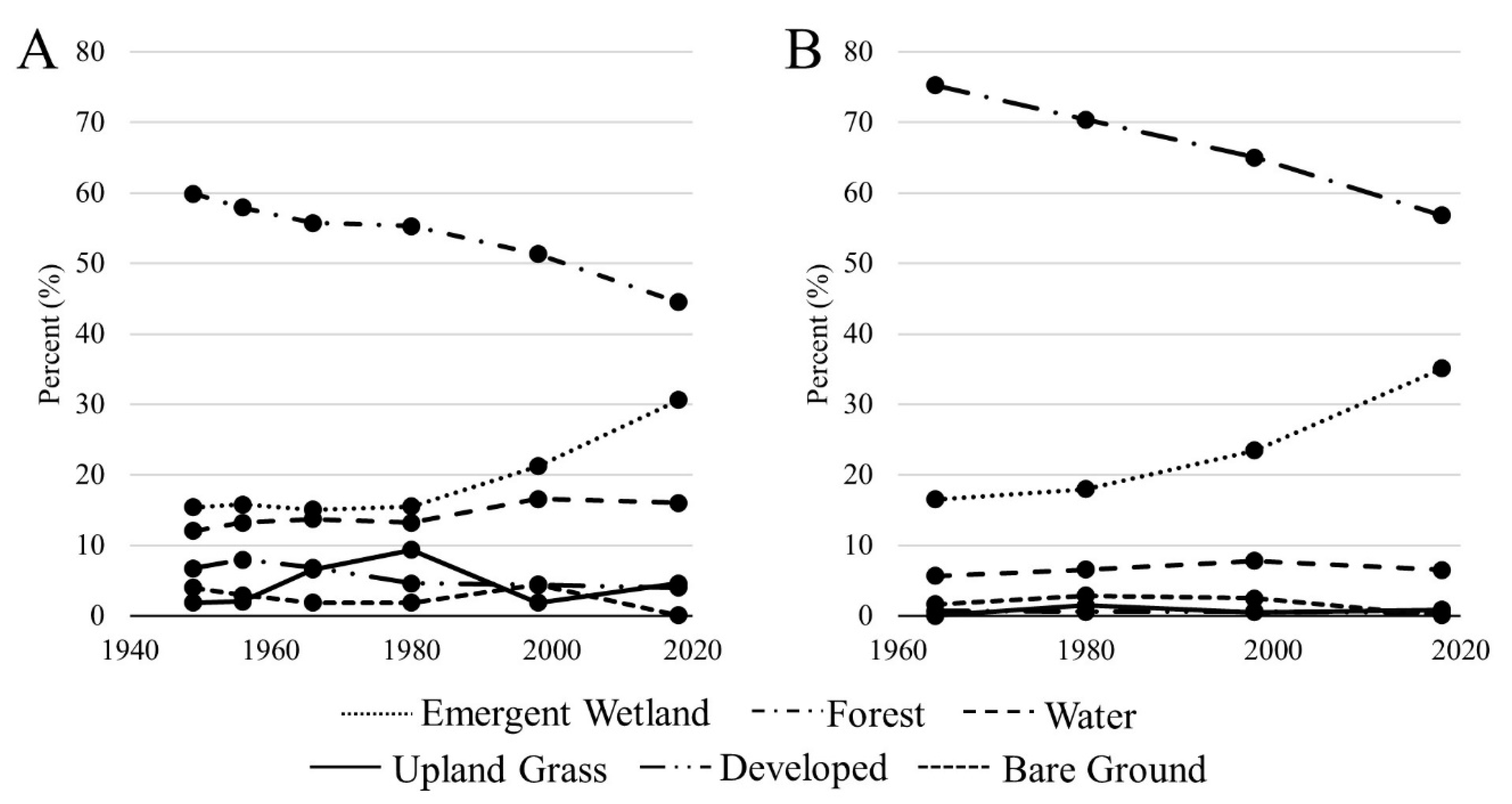
The dominant cover type in both Smith Creek and Town Creek was forest where coverage ranged from 60% in 1949 to 45% in 2018 for Smith Creek and 75% in 1964 to 57% in 2018 for Town Creek (Figure 5). Emergent wetland was the next dominant, ranging from 15% in 1949 to 30% in 2018 for Smith Creek and 17% in 1964 to 35% in 2018 for Town Creek. Developed, bare ground, and upland grass did not change throughout Town Creek yet varied in Smith Creek due to periods of construction and timber harvest.
In 1949, the dominant land cover type in all segments of Smith Creek was forest, which ranged from 35% in the lower segment to 91% in the upper segment; however, by 2018 emergent wetland was largest at 48% in the lower segment while forest still dominated the middle (45%) and upper (74%) segments (see Supplementary Figure S6 for statistics by creek segment). Overall, from 1949 to 2018, forest consistently declined in all segments with the greatest loss in the middle segment (21%) and upper segment (17%) and less loss (11%) in the lower segment. Emergent wetland was located only in the lower segment in 1949, 1956, and 1966, but in 1980 emergent wetland was in the middle segment and in 2018 it was in the upper segment.
In 1964, the dominant land cover type in the lower creek segment of Town Creek was emergent wetland (53%) while forest dominated in the other creek segments (lower-mid at 74%, upper-mid at 95%, upper at 91%); however, by 2018, emergent wetland was the dominant land cover in the lower (57%) and lower-mid (58%) segments while forest still dominated in upper-mid (60%) and upper (93%) segments (see Supplementary Figure S6 for statistics by creek segment). Overall, from 1964 to 2018, forests declined in the lower, lower-mid, and upper-mid creek segments and experienced no change in the upper segment with the greatest loss in the lower-mid (43%) and upper-mid (36%) segments. Emergent wetland was located only in the lower and lower-mid segments in 1964, but in 1980 emergent wetland was in the upper-mid segment and in 2018 it was in the upper segment.
3.3.2. Greatest Change: Loss of Forest, Change in Emergent Wetland, and Gain in Water
For both Smith Creek and Town Creek, the greatest change in land cover was forest to emergent wetland (Figure 6). Overall, Smith Creek had 14% (67.5 ha) of the study area change from forest to emergent wetland from 1949 to 2018 and Town Creek had 18% (272.3 ha) of the study area change from 1964 to 2018. Specifically, in Smith Creek, the greatest net gain in emergent wetland from forest occurred in the middle segment (26%) followed by the lower segment (18%) (see Supplementary Table S3 for summary stats by creek segment). In Town Creek the greatest net gain in emergent wetland from forest occurred in the lower-mid (43%) and upper-mid (35%) segments (see Supplementary Table S4 for summary stats by creek segment). Additionally, the rate of change from forest to emergent wetland for both creeks moved upstream over time (Supplementary Tables S3 and S4). For Smith Creek, the greatest rate of change occurred in the lower creek segment from 1980–1998 and in the middle and upper creek segments from 1998–2018. Similarly, for Town Creek, the greatest rate of change occurred from 1964–1980 in the lower segment, 1980–1998 in the lower-mid segment, and 1998–2018 in the upper-mid and upper segments.
Both Smith Creek and Town Creek also experienced a transition from emergent wetland to water. Overall, Smith Creek experienced a 3% net increase in water from emergent wetland where the greatest transition occurred in the lower creek segment from 1980 to 1998 followed by the middle creek segment from 1998 to 2018 (Supplementary Table S3). Similarly, Town Creek experienced a 1% net increase in water from emergent wetland where the greatest change occurred in the lower-mid segment from 1964 to 1980 (Supplementary Table S4).
Across both Smith Creek and Town Creek, there was a greater loss of forest to emergent wetland and emergent wetland to water than gain in emergent wetland from forest and water from emergent wetland (Figure 7). For Smith Creek, there was a significant loss in forest to emergent wetlands in three time periods (1966–1980, 1980–1998, and 1998–2018) and only occurred in the middle creek segment. The loss from 1966–1980 coincided with the appearance of emergent wetlands in the middle creek segment in 1980, while the loss from 1980–1998 and 1998–2018 was consistent with the high land cover change (11.28% from 1980–1998 and 12.94% of 1998–2018) occurring during these time periods (Supplementary Table S3). For Town Creek, there was a significant loss in forest to emergent wetland in two time periods (1980–1998 and 1998–2018). The loss from 1980–1998 coincided with the appearance of emergent wetlands in the upper-mid segment in 1998 and the loss from 1998–2018 coincided with the appearance of emergent wetlands in the upper creek segment in 2018.
3.3.3. Upstream Movement of the Forest/Emergent Wetland Boundary
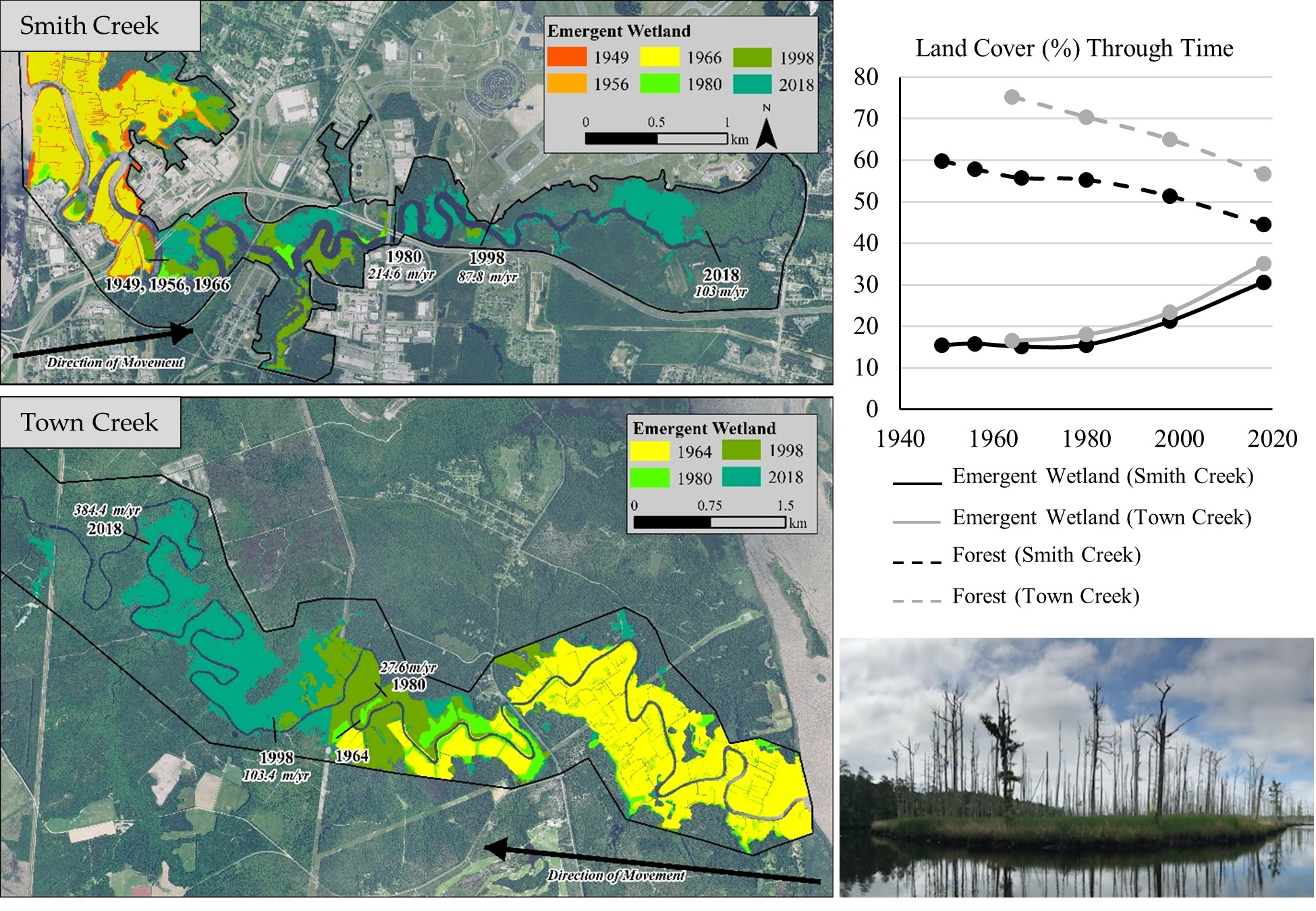
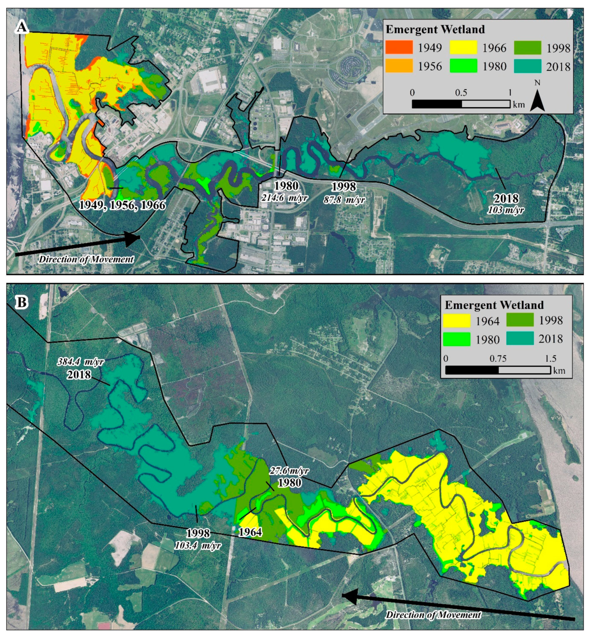
At Smith Creek, the average elevation at the headwater was 24.4 m and 2.2 m at the mouth for a slope of 1.3 m/km and Town Creek was 59.3 m at the headwater and 2.0 m at the mouth for a slope of 1.07 m/km. Using 2.47 mm/yr RSLR in Wilmington for the 20th century [14] and each creek slope, the rate of tidal extension would be 1.9 m/yr for Smith Creek and 2.3 m/yr for Town Creek. Using these rates of extension, the forest/emergent wetland boundary was expected to move 0.13 km from 1949 to 2018 on Smith Creek and 0.12 km from 1964 to 2018 on Town Creek. However, the forest/emergent wetland boundary moved 6.65 km upstream on Smith Creek and 10 km upstream on Town Creek (Figure 8), resulting in a rate of migration that ranged from 87.8 to 214.6 m/yr on Smith Creek and 27.6 to 384.4 m/yr on Town Creek (Table 4).
4. Discussion
4.1. Compare Land Cover Change and Physical Geography Characteristics
This research confirmed the hypothesis that there has been a change in the distribution of wetlands where forested areas have transitioned to emergent wetlands and emergent wetlands have transitioned to water. There was also an upstream movement of the forest/emergent boundary. In comparing the two creeks, the percentage of transition from forest to emergent wetland was significantly different (P = 0.01) between Smith Creek and Town Creek, but conversion to water (P = 0.69) and the rate of saltwater migration up the creeks was not significantly different (P = 0.19).
Based on the literature, and close proximity, it was hypothesized that the physical geography characteristics would not be different between Smith Creek and Town Creek; however, there were several metrics that were significantly different: (1) creek width through time (P = 0.0006), (2) floodplain width (P = 0.0004), (3) sinuosity (P = 0.0584), and (4) floodplain elevation (P = 0.0898). Average change in creek width (P = 0.110) and average water level (P = 0.223) were not significantly different between the two study areas, but these are not expected to vary in short distances, so it is not surprising that these were not significantly different. The significant differences in physical characteristics are important because they illustrate how tidal creeks are not all the same; they vary in size, shape, topography, etc., even though they are in close proximity and are within the same physiographic province (coastal plain).
Lastly, it was hypothesized that physical geography characteristics were related to changes in wetlands; however, only three metrics at Smith Creek (sinuosity, change in creek width, and floodplain elevation) and two metrics at Town Creek (sinuosity and change in creek width) were related to the change from emergent wetland to water. There are very few studies that have investigated a relationship between land cover, wetland change, and metrics that describe the physical geography of a location. Other than erosion/accretion related to shoreline change and area of coastal features [60,61,62], most studies do not holistically investigate changing coastal riverine dynamics and land cover change. Therefore, one of the main contributions of this research was to investigate these metrics to see if there is a pattern and to measure the spatial and statistical relationships among several characteristics through time.
4.2. Salinity, Water Level, and Saltwater Migration Upstream
The salinity measurements recorded in this study (from 10 August 2018 to 9 September 2018) were similar to the monthly salinity data from 2005–2016 reported by the Lower Cape Fear River Program and from 2000–2010 reported by the US Army Corps of Engineers (USACOE) monitoring of the Wilmington Harbor [16,63]. However, the salinity data collected in this study did not reach the peak salinities identified in either study [16,63]. The Lower Cape Fear River program reported peak salinities during the late fall and winter and the lowest salinity in spring and summer [63]. Salinity values are primarily driven by river discharge and precipitation [16]. Daily precipitation data in Wilmington (obtained from the National Centers for Environmental Information [64]) for the same period that our instruments were within the creeks showed that there was no correlation between salinity and daily precipitation (Figure 9); however, river discharge data from the USGS gauging station (station 02105769) at Lock and Dam 1 (see location in Figure 1) [65] was correlated with salinity where low river discharge related to higher salinity (Figure 9). Given these results, salinity in these creeks is likely driven by Cape Fear River discharge and precipitation, which is consistent with the finding from the USACOE long-term monitoring study [16].
The rate at which saltmarsh migrated upstream (87.8 to 214.6 m/yr on Smith Creek and 27.6 to 384.4 m/yr on Town Creek) far exceeded the anticipated rate that saltwater should migrate upstream due to RSLR (1.9 m/yr on Smith Creek and 2.3 m/yr on Town Creek) and, therefore, RSLR cannot be the sole factor dominating wetland change in these two tidal creeks. Additionally, the tidal range in Wilmington increased 0.41 m since the installation of the NOAA tide gauge in 1936; however, only 0.202 m can be attributed to RLSR and, therefore, the remaining 0.208 m was likely the result of the frequent dredging in the Cape Fear River, which has increased channel depth 9.1 m since 1871. Dredging increases the volume of water and, therefore, leads to movement of the saltwater wedge further up the estuary. This migration of salinity mimics the effects of RSLR, which pushes tides and salinity upstream. Therefore, given that we calculated an increasing tidal range through time using daily water levels from 1936 to 2018 [14] and there are documented dredging activities, it is likely that the combination of increased tidal range through RSLR and dredging activities enabled saltier water to move further inland, including up the tidal creeks, resulting in vegetation transitioning from forest to emergent wetland.
4.3. Sources of Error
The ability to document historic wetland distributions through aerial photography has previously been successful for coastal wetlands [7,19,41] and barrier islands [42]. When conducting heads-up digitizing, there are many sources of potential error including rectification, interpretation, and digitization. In this study, the rectification (0.83–4.67 m) and digitization errors (0.62–1.52 m) were similar to the rectification (0.5–3 m) and digitization errors (0.55–3 m) from other studies in coastal habitats [49,50,51,52]. When mapping intertidal habitats, images ideally should be acquired during the same tidal phase and phenological stage to accurately delineate vegetation. While image acquisition date and time was available for the WV-2 imagery, it was unavailable for the aerial photography, making it difficult to account for the tidal regime/height during the time of image acquisition. However, we can assume that the aerial photography was obtained during mid to high tide due to the absence of any mud flats within the water bodies. Second, if imagery dates were obtained during different tidal phases, the location of “change” through time would be consistent along the creek boundary between water and non-water (e.g., emergent wetland, forest). However, this was not the case as both Smith Creek and Town Creek experienced varying amounts of change throughout the creek between imagery dates. Therefore, we can conclude that the tidal regimes were close between image dates, and transitions between land cover types (e.g., emergent wetlands to water) represent true transitions rather that misidentified transitions due to the influence of tides. Third, the phenological stage during image acquisition poses an issue for bald cypress trees, which lose their needlelike leaves in the winter, making it difficult to decipher dead versus deciduous trees. This issue arose for the 1998 Digital Orthophoto Quarter-Quads (DOQQs) taken in January, resulting in potentially misclassified vegetation. However, the 1998 imagery were compared to imagery from the early 2000s that was obtained during leaf-on conditions, which verified the land cover designations from the 1998 imagery. Lastly, the classification accuracy of the WorldView-2 imagery (98% for Smith Creek and 96% for Town Creek) was similar to other wetland classification studies [56,57], indicating that WV-2 imagery is a reliable source for mapping coastal wetlands in this study area.
4.4. Future Work
This research initiated the investigation into whether there were changes in wetlands and when they occurred, and the rate of migration upstream as an indication of increasing saltwater. The next step in this research is to (1) replicate this work on sites that do not have any influence from dredging, (2) investigate urbanization and deforestation and the relationship with sedimentation rates, (3) incorporate many more dates of recent satellite imagery in order to decipher the relationship with seasonal weather, and (4) perform additional field work to measure salinity and the influence of groundwater and surface water to link this water level and saltwater extent. These four items are currently being developed with a larger team of multidisciplinary researchers.
We purposely selected sites that had nearby dredging because these activities dramatically mimic a rising sea level and, if we documented the impacts on vegetation under these conditions, then other tidal creeks that have no influence of dredging (i.e., tributaries of the New River and White Oak River) may provide insight into changing land cover that is directly related to rising sea level.
This study utilized six dates of imagery at one creek and four dates at the other creek. So, now that we have identified habitat changes, migration rate of saltmarsh moving upstream, and changes in water level, this work can be expanded to many dates of imagery that could provide more detailed spatial and temporal analysis of land cover transitions, rate of upstream movement of the emergent wetland/forest boundary, and comparison with seasonal weather. Thus, imagery sources with greater spatial, spectral, and temporal resolutions (i.e., WorldView-2/3, NAIP, PlanetScope, QuickBird, and IKONOS) will provide more image acquisition dates and increased measurement of when land cover transitions occurred. Further, with the greater spectral and spatial resolution, species-level vegetation change could be feasible [44,47,56].
Lastly, additional research could investigate tides and salinity through time and space in greater detail by installing devices at more locations and for a longer duration. This would allow for a greater understanding of temporal (daily, monthly, seasonal) and spatial changes as well as the drivers of salinity from both a groundwater and surface water perspective. This combination of increased spatial and temporal mapping, replication at other sites, and further understanding the influence of weather and salinity will greatly increase our understanding of the processes and resulting land cover changes under a rising sea level.
5. Conclusions
This study utilized aerial photography and satellite imagery to map tidal creek habitats with high spatial accuracy. The results identified habitat change in tidal creeks, migration of emergent marsh upstream, and the relationship with physical geography metrics such as floodplain elevation, creek sinuosity, average change in creek width, average water level, river discharge, and precipitation. There have been other case studies investigating wetland transition/loss along tidal creeks of the Cape Fear River [19,20]; however, this is the first multi-decadal investigation in the Cape Fear River that sheds light into when and where change occurred.
Results from this study identified substantial change in the distribution of wetlands since the mid-1900s where (1) 67.85 ha (14%) on Smith Creek and 272 ha (18%) on Town Creek transitioned from forest to emergent wetland, (2) the rate of transition was the greatest since 1980, (3) the forest/emergent wetland boundary migrated upstream 6.65 km at Smith Creek and 10 km at Town Creek, (4) the transition from forest to emergent wetland was significantly different between the two creeks, and (5) sinuosity, change in creek width, and floodplain elevation were significantly related to the change in wetlands. Ultimately, this research provides valuable insight into the location and timing of forest and wetland transitions in coastal tidal creeks, describes a methodology for identifying change, and relates this with physical geography characteristics.
Supplementary Materials
The following are available online at https://0-www-mdpi-com.brum.beds.ac.uk/2072-4292/12/7/1141/s1: Figure S1: Physical geography metrics calculated for each study area. Figure S2: Location of upstream and downstream locations used to calculate creek slope. Figure S3: Example accuracy assessment where randomly selected polygons were redigitized and the distance between the original and redigitized lines was used to calculate digitizing accuracy. Figure S4. Change in creek width. Figure S5: Geographic trend in creek metrics. Figure S6: Percent land cover type through time by creek segment. Table S1: Average difference in time (hrs:mins) between high tide at the NOAA tide gauge in Wilmington to instruments located in Smith Creek and Town Creek. Table S2: Average creek width (m) through time for Smith Creek and Town Creek. Table S3: Net change (%) between forest to emergent and emergent to water for each creek segment in Smith Creek. Table S4: Net change (%) between forest to emergent and emergent to water for each creek segment in Town Creek.
Author Contributions
The following contributions were made to this publication: J.N.H. conceptualized the project while J.L.M. and J.N.H designed the methodology; J.L.M. used remote sensing and GIS software, conducted the formal analysis, and created visualizations while J.L.M. and J.N.H collaborated on the project investigation, data curation, and writing the manuscript. J.N.H provided supervision and project administration and funding acquisition was performed by J.L.M. and J.N.H. All authors have read and agreed to the published version of the manuscript.
Funding
This research was partially funded by the Geological Society of America, Robert D. Hatcher/Research Award, and the American Association of Geographers Applied Geography Specialty Group Student Research Fellowship.
Acknowledgments
The authors would like to thank the Department of Earth and Ocean Sciences, University of North Carolina Wilmington, for providing a Trimble RTK, pressure transducers, and salinity gauges; Britton Baxley, Yvonne Marsan, Jeff Edwards, and Sara Chahin for assistance with field work; the Army Corp of Engineers for providing WorldView-2 imagery; Britton Baxley for preprocessing the WorldView-2 imagery; Jordan Skinner and James Olshan for assistance with digitizing aerial photography; and Narcisa Pricope for a software license to use eCognition.
Conflicts of Interest
The authors declare no conflict of interest and the funders had no role in the design of the study; in the collection, analyses, or interpretation of data; in the writing of the manuscript, or in the decision to publish the results.
References
- Weigert, R.G.; Freeman, B.J. Tidal Salt Marshes of the Southeast Atlantic Coast: A Community Profile; U.S. Fish and Wildlife Service: Washington, DC, USA, 1990; p. 80.
- Stammermann, R.; Piasecki, M. Influence of sediment availability, vegetation, and sea level rise on the development of tidal marshes. J. Coast. Res. 2012, 28, 1536–1549. [Google Scholar] [CrossRef]
- Alber, M.; Swenson, E.; Adamowicz, S.; Mendelssohn, I. Salt Marsh Dieback: An overview of recent events. Estuar. Coast. Shelf Sci. 2008, 80, 1–11. [Google Scholar] [CrossRef]
- Mudd, S.; Howell, S.; Morris, J. Impact of dynamic feedbacks between sedimentation, sea-level rise, and biomass production on near-surface marsh stratigraphy and carbon accumulation. Estuar. Coast. Shelf Sci. 2009, 82, 377–389. [Google Scholar] [CrossRef]
- Sanger, D.; Parker, C. Guide to Salt Marshes and Tidal Creeks of the Southeastern United States; South Carolina Department of Natural Resources: Charleston, SC, USA, 2016.
- Dame, R.; Alber, M.; Allen, D.; Mallin, M.; Montague, C.; Lewitus, A.; Chalmers, A.; Gardner, R.; Gilman, C.; Kjerfve, B.; et al. Estuaries of the south Atlantic coast of North America: Their geographical signatures. Estuaries 2000, 23, 793–819. [Google Scholar] [CrossRef]
- Higinbotham, C.B.; Alber, M.; Chalmers, A.G. Analysis of tidal marsh vegetation patterns in two Georgia estuaries using aerial photography and GIS. Estuaries 2004, 27, 670–683. [Google Scholar] [CrossRef]
- Kirwan, M.L.; Gedan, K.B. Sea-level driven land conversion and the formation of ghost forests. Nat. Clim. Chang. 2019, 9, 450–457. [Google Scholar] [CrossRef] [Green Version]
- Kirwan, M.L.; Gedan, K.B. Author Correction: Sea-level driven land conversion and the formation of ghost forests. Nat. Clim. Chang. 2019, 9, 726. [Google Scholar] [CrossRef]
- McCarthy, M.J.; Dimmitt, B.; Muller-Karger, F.E. Rapid Coastal Forest Decline in Florida’s Big Bend. Remote Sens. 2018, 10, 1721. [Google Scholar] [CrossRef] [Green Version]
- Zervas, C. Sea Level Variations of the United States 1854–2006; NOAA Technical Report NOS CO-OPS 053; NOAA: Silver Springs, FL, USA, 2009. [Google Scholar]
- Church, J.A.; Clark, P.U.; Cazenave, A.; Gregory, J.M.; Jevrejeva, S.; Levermann, A.; Merrifield, M.A.; Milne, G.A.; Nerem, R.S.; Nunn, P.D.; et al. Sea Level Change. In Climate Change 2013: The Physical Science Basis. Contribution of Working Group I to the Fifth Assessment Report of the Intergovernmental Panel on Climate Change; Stocker, T.F., Qin, D., Plattner, G.-K., Eds.; Cambridge University Press: New York, NY, USA, 2013; pp. 1137–1216. [Google Scholar]
- Sweet, W.V.; Kopp, R.E.; Weaver, C.P.; Obeysekera, J.; Horton, R.M.; Thieler, E.R.; Zervas, C. Global and Regional Sea Level Rise Scenarios for the United States; NOAA: Silver Springs, FL, USA, 2017. [Google Scholar]
- NOAA. Tides and Currents. Available online: https://tidesandcurrents.noaa.gov/ (accessed on 1 May 2019).
- Odum, W.E.; Smith, T.J.; Hoover, J.K.; McIvor, C.C. The Ecology of Tidal Freshwater Marshes of the United States East Coast: A Community Profile; FWS/OBS-83/17; U.S. Fish Wildlife Service: Washington, DC, USA, 1984; p. 177.
- USACOE. Monitoring Effects of a Potential Increased Tidal Range in the Cape Fear River Ecosystem Due to Deepening Wilmington Harbor, North Carolina Year 10: June 1, 2009–May 31; USACE: Wilmington, NC, USA, 2010.
- USACOE. Draft Integrated Feasibility Report and Environmental Assessment, Wilmington Harbor Navigation Improvements; USACE: Wilmington, NC, USA, 2014.
- USACOE. Long-Term Maintenance of Wilmington Harbor, North Carolina; USACE: Wilmington, NC, USA, 1988.
- Hackney, C.; Yelverton, F. Effects of Human Activities and Sea Level Rise on Wetland Ecosystems in the Cape Fear River Estuary, North Carolina, USA. In Wetlands Ecology and Management: Case Studies; Whigham, D.F., Good, R.E., Evet, J., Eds.; Springer: Dordrecht, The Netherlands, 1990; pp. 55–63. [Google Scholar]
- Hackney, C.T.; Avery, G.B. Tidal Wetland Community Response to Varying Levels of Flooding by Saline Water. Wetlands 2015, 35, 227–236. [Google Scholar] [CrossRef]
- North Carolina Department of Environment Health and Natural Resources. Common Wetland Plants of North Carolina; North Carolina Department of Environment Health and Natural Resources: Raleigh, NC, USA, 1997.
- Perry, J.E.; Hershner, C.H. Temporal changes in the vegetation patterns in a tidal freshwater marsh. Wetlands 1999, 19, 90–99. [Google Scholar] [CrossRef]
- Swarth, C.W.; Delgado, P.; Whigham, D.F. Vegetation Dynamics in a Tidal Freshwater Wetland: A Long-Term Study at Differing Scales. Estuaries Coasts 2013, 36, 559–574. [Google Scholar] [CrossRef]
- US Census Bureau. Available online: https://factfinder.census.gov/faces/nav/jsf/pages/index.xhtml (accessed on 1 January 2020).
- Davis, R.A.; Fitzgerald, D.M. Beaches and Coasts; Blackwell Science Ltd.: Hoboken, NJ, USA, 2004. [Google Scholar]
- University of North Carolina Wilmington. Lower Cape Fear River Program. Available online: https://uncw.edu/cms/aelab/lcfrp/ (accessed on 1 June 2019).
- USFWS. National Wetlands Inventory. Available online: https://www.fws.gov/wetlands/ (accessed on 1 November 2017).
- Cowardin, L.M.; Carter, V.; Golet, F.C.; LaRoe, E.T. Classification of Wetlands and Deepwater Habitats of the United States; FWS/OBS-79/31; U.S. Fish Wildlife Service: Washington, DC, USA, 1979.
- ONSET. HOBO 250-ft Depth Water Level Data Logger. Available online: https://www.onsetcomp.com/products/data-loggers/u20-001-03 (accessed on 1 May 2018).
- ONSET. HOBOware Pro. Available online: https://www.onsetcomp.com/products/software/bhw-pro (accessed on 1 May 2018).
- ONSET. HOBOware Pro Barometric Compensation Assistant User’s Guide. Available online: https://www.onsetcomp.com/files/manual_pdfs/Barometric-Compensation-Assistant-Users-Guide-10572.pdf (accessed on 1 May 2018).
- ONSET. HOBO Salt Water Conductivity/Salinity Data Logger. Available online: https://www.onsetcomp.com/products/data-loggers/u24-002-c (accessed on 1 May 2018).
- ONSET. HOBOware Pro Conductivity Assistant User’s Guide. Available online: https://www.onsetcomp.com/files/manual_pdfs/Conductivity-Assistant-Users-Guide-15019.pdf (accessed on 1 May 2018).
- USGS. National Hydrography Dataset. Available online: https://www.usgs.gov/core-science-systems/ngp/national-hydrography (accessed on 1 June 2019).
- FEMA. FEMA Flood Map Service Center. Available online: https://msc.fema.gov/portal/home (accessed on 9 November 2017).
- NC Department of Emergency Management. QL2 LiDAR. Available online: https://sdd.nc.gov/sdd/ (accessed on 1 May 2018).
- Ensign, S.H.; Noe, G.B. Tidal extension and sea-level rise: Recommendations for a research agenda. Front. Ecol. Environ. 2018, 16, 37–43. [Google Scholar] [CrossRef]
- NHC. Orthophotos. Available online: https://maps.nhcgov.com/ (accessed on 1 June 2018).
- USGS. Aerial Photo Single Frame. Available online: https://earthexplorer.usgs.gov/ (accessed on 1 October 2018).
- USGS. Digital Orthophoto Quadrangle (DOQs). Available online: https://earthexplorer.usgs.gov/ (accessed on 1 October 2018).
- Hackney, C.T.; Brady, S.; Stemmy, L.; Boris, M.; Dennis, C.; Hancock, T.; Obryon, M.; Tilton, C.; Barbee, E. Does intertidal vegetation indicate specific soil and hydrologic conditions. Wetlands 1996, 16, 89–94. [Google Scholar] [CrossRef]
- Halls, J.; Kraatz, L. A Spatio-Temporal Assessment of Back-Barrier Salt Marsh Change: A Comparison of Multidate Aerial Photography and Spatial Landscape Indices. In Proceedings of the ISPRS Commission VII Mid-term Symposium Remote Sensing: From Pixels to Processes, Enschede, The Netherlands, 8–11 May 2006. [Google Scholar]
- McCarthy, M.; Halls, J. Habitat Mapping and Change Assessment of Coastal Environments: An Examination of WorldView-2, QuickBird, and IKONOS Satellite Imagery and Airborne LiDAR for Mapping Barrier Island Habitats. ISPRS Int. J. Geo-Inf. 2014, 3, 297–325. [Google Scholar] [CrossRef] [Green Version]
- Halls, J.; Costin, K. Submerged and Emergent Land Cover and Bathymetric Mapping of Estuarine Habitats Using WorldView-2 and LiDAR Imagery. Remote Sens. 2016, 8, 718. [Google Scholar] [CrossRef] [Green Version]
- Hassan, N.; Hamid, J.R.A.; Adnan, N.A.; Jaafar, M. Delineation of wetland areas from high resolution WorldView-2 data by object-based method. In Proceedings of the 8th International Symposium of the Digital Earth (ISDE), Univ Teknologi Malaysia, Inst Geospatial Sci & Technol, Kuching, Malaysia, 26–29 August 2013. [Google Scholar]
- Rapinel, S.; Clement, B.; Magnanon, S.; Sellin, V.; Hubert-Moy, L. Identification and mapping of natural vegetation on a coastal site using a Worldview-2 satellite image. J. Environ. Manag. 2014, 144, 236–246. [Google Scholar] [CrossRef] [PubMed] [Green Version]
- Lane, C.R.; Liu, H.X.; Autrey, B.C.; Anenkhonov, O.A.; Chepinoga, V.V.; Wu, Q.S. Improved Wetland Classification Using Eight-Band High Resolution Satellite Imagery and a Hybrid Approach. Remote Sens. 2014, 6, 12187–12216. [Google Scholar] [CrossRef] [Green Version]
- USDA. National Agriculture Imagery Program (NAIP). Available online: https://www.fsa.usda.gov/programs-and-services/aerial-photography/imagery-programs/naip-imagery/ (accessed on 1 October 2018).
- Cowart, L.; Walsh, J.P.; Corbett, D.R. Analyzing estuarine shoreline change: A case study of Cedar Island, North Carolina. J. Coast. Res. 2010, 26, 817–830. [Google Scholar] [CrossRef]
- Cowart, L.; Corbett, D.R.; Walsh, J.P. Shoreline Change along Sheltered Coastlines: Insights from the Neuse River Estuary, NC, USA. Remote Sens. 2011, 3, 1516–1534. [Google Scholar] [CrossRef] [Green Version]
- Currin, C.; Davis, J.; Baron, L.C.; Malhotra, A.; Fonseca, M. Shoreline Change in the New River Estuary, North Carolina: Rates and Consequences. J. Coast. Res. 2015, 31, 1069–1077. [Google Scholar] [CrossRef]
- Fletcher, C.; Rooney, J.; Barbee, M.; Lim, S.C.; Richmond, B. Mapping shoreline change using digital orthophotogrammetry on Maui, Hawaii. J. Coast. Res. 2003, 38, 106–124. [Google Scholar]
- Digital Globe. WorldView-2. Available online: https://www.digitalglobe.com/ (accessed on 1 January 2019).
- Harris Geospatial Solutions. Fast line-of-sight atmospheric analysis of hypercubes (FLAASH). Available online: https://www.harrisgeospatial.com/docs/FLAASH.html (accessed on 15 May 2019).
- Trimble. eCognition Essentials, Version 1.3. Available online: http://www.ecognition.com/ (accessed on 21 June 2018).
- Gilmore, M.S.; Wilson, E.H.; Barrett, N.; Civco, D.L.; Prisloe, S.; Hurd, J.D.; Chadwick, C. Integrating multi-temporal spectral and structural information to map wetland vegetation in a lower Connecticut River tidal marsh. Remote Sens. Environ. 2008, 112, 4048–4060. [Google Scholar] [CrossRef]
- Byrd, K.B.; Ballanti, L.; Thomas, L.; Nguyen, D.; Holmquist, J.R.; Simard, M.; Windham-Myers, L. A remote sensing-based model of tidal marsh aboveground carbon stocks for the conterminous United States. ISPRS J. Photogramm. Remote Sens. 2018, 139, 17. [Google Scholar] [CrossRef]
- Wolf, A.F. Using Worldview-2 Vis-NIR Multispectral Imagery to Support Land Mapping and Feature Extraction Using Normalized Difference Index Ratios. In Proceedings of the Annual Conference on Algorithms and Technologies for Multispectral, Hyperspectral, and Ultraspectral Imagery XVIII, Baltimore, MD, USA, 23–27 April 2012. [Google Scholar]
- Pontius, R.G.; Shusas, E.; McEachern, M. Detecting important categorical land changes while accounting for persistence. Agric. Ecosyst. Environ. 2004, 101, 251–268. [Google Scholar] [CrossRef]
- Al-Nasrawi, A.K.M.; Hamylton, S.M.; Jones, B.G. An assessment of anthropogenic and climatic stressors on estuaries using a spatio-temporal GIS-modelling approach for sustainability: Towamba estuary, southeastern Australia. Environ. Monit. Assess. 2018, 190, 26. [Google Scholar] [CrossRef]
- Jangir, B.; Satyanarayana, A.N.V.; Swati, S.; Jayaram, C.; Chowdary, V.M.; Dadhwal, V.K. Delineation of spatio-temporal changes of shoreline and geomorphological features of Odisha coast of India using remote sensing and GIS techniques. Nat. Hazards 2016, 82, 1437–1455. [Google Scholar] [CrossRef]
- Ramirez-Cuesta, J.M.; Rodriguez-Santalla, I.; Gracia, F.J.; Sanchez-Garcia, M.J.; Barrio-Parra, F. Application of change detection techniques in geomorphological evolution of coastal areas. Example: Mouth of the River Ebro (period 1957-2013). Appl. Geogr. 2016, 75, 12–27. [Google Scholar] [CrossRef]
- Mallin, M.A.; McIver, M.R.; Merrit, J.F. Environmental Assessment of the Lower Cape Fear River System, 2015; UNCW Center for Marine Science: Wilmington, NC, USA, 2016; p. 48. [Google Scholar]
- NOAA National Centers for Environmental Information. Climate Data Online. Available online: https://www.ncdc.noaa.gov/cdo-web/ (accessed on 15 May 2019).
- USGS. National Water Information System Web Interface. Available online: https://nwis.waterdata.usgs.gov/nwis (accessed on 1 June 2019).
Figure 1.
The study area includes Smith Creek and Town Creek, located in Southeastern North Carolina where (A) is the general location of North Carolina in the Eastern USA, (B) the Cape Fear River estuary and the location of the two creeks in this study, and (C) Smith Creek and (D) Town Creek with locations of field equipment and creek segments. Data Sources: Hackney and Avery 1990 [19] and Hackney et al., 2015 [20] (historic research sites), Lower Cape Fear River Program and US Army Corp of Engineers (historic salinity sites) [16,26], NOAA (tide stations) [14], and US Fish and Wildlife Service (National Wetlands Inventory (NWI) wetlands) [27].

Figure 2.
Conceptual model of coastal riverine wetlands in southeastern North Carolina describing the differences in salinity and species that occupy each type of wetland. Adapted from Cowardin et al., 1979 [28], and Odum et al., 1984 [15].

Figure 3.
Generalized workflow involved mapping land cover, computing physical geography metrics, and analyzing change through time.
Figure 3.
Generalized workflow involved mapping land cover, computing physical geography metrics, and analyzing change through time.

Figure 4.
Aerial photography and WorldView-2 imagery for a portion of Smith Creek where (A) is aerial photography from 1949 to 1998 and WorldView-2 from 2018 and (B) is classified land cover from 1949 to 2018.
Figure 4.
Aerial photography and WorldView-2 imagery for a portion of Smith Creek where (A) is aerial photography from 1949 to 1998 and WorldView-2 from 2018 and (B) is classified land cover from 1949 to 2018.

Figure 5.
Percent land cover type (emergent wetland, forest, water, upland grass, developed, and bare ground) through time for (A) Smith Creek and (B) Town Creek.
Figure 5.
Percent land cover type (emergent wetland, forest, water, upland grass, developed, and bare ground) through time for (A) Smith Creek and (B) Town Creek.

Figure 6.
Land cover transitions from forest to emergent wetland (A,B) and emergent wetland to water (C,D) for Smith Creek (A,C) and Town Creek (B,D).
Figure 6.
Land cover transitions from forest to emergent wetland (A,B) and emergent wetland to water (C,D) for Smith Creek (A,C) and Town Creek (B,D).

Figure 7.
Land cover change (in percent) between forest and emergent wetland (A,B) and emergent wetland and water (C,D) for Smith Creek (A,C) and Town Creek (B,D). Transitions indicated with “*” were significantly more than expected.
Figure 7.
Land cover change (in percent) between forest and emergent wetland (A,B) and emergent wetland and water (C,D) for Smith Creek (A,C) and Town Creek (B,D). Transitions indicated with “*” were significantly more than expected.

Figure 8.
Emergent wetlands through time, where the upstream extent is shown by year and annotated with the rate of movement (m/yr) from the proceeding time period for (A) Smith Creek and (B) Town Creek.
Figure 8.
Emergent wetlands through time, where the upstream extent is shown by year and annotated with the rate of movement (m/yr) from the proceeding time period for (A) Smith Creek and (B) Town Creek.

Figure 9.
Salinity for Smith Creek (downstream location) and Town Creek compared with daily precipitation [64] and river discharge [65].


Table 1.
Imagery dates, sources, spectral characteristics, and spatial scale/resolution.
| Year | Month/Date | Data Type | Provider | Spectral | Spatial | |
|---|---|---|---|---|---|---|
| Smith Creek | 1949 | 4/19, 12/1 | Aerial Photography | New Hanover County | BW | 1”: 1320′ |
| 1956 | 3/23, 3/25, 6/4 | Aerial Photography | New Hanover County | BW | 1”: 1320′ | |
| 1966 | 3/18, 3/20 | Aerial Photography | New Hanover County | BW | 1”: 1320′ | |
| 1980 | 10/1 | Aerial Photo Single Frame | US Geological Survey | CIR | 1:80,000 | |
| 1998 | 1/26 | DOQQ | US Geological Survey | CIR | 1 m | |
| 2016 | 5/16, 6/12 | NAIP Orthophotography* | USDA Farm Service Agency | RGBN | 1 m | |
| 2018 | 7/19 | WorldView-2 | Digital Globe | 8-band | 2.29 m | |
| Town Creek | 1964 | 4/1 | Aerial Photo Single Frame | US Geological Survey | BW | 1:50,000 |
| 1980 | 10/1 | Aerial Photo Single Frame | US Geological Survey | CIR | 1:80,000 | |
| 1998 | 1/26, 2/25 | DOQQ | US Geological Survey | CIR | 1 m | |
| 2016 | 5/16, 6/12 | NAIP Orthophotography* | USDA Farm Service Agency | RGBN | 1 m | |
| 2018 | 7/19 | WorldView-2 | Digital Globe | 8-band | 2.29 m |
*2016 NAIP Orthophotography was used for rectification of historical aerial photography.
Table 2.
Sinuosity, average creek width, average change in creek width through time, average floodplain width, and average floodplain elevation, for Smith Creek and Town Creek.
Table 2.
Sinuosity, average creek width, average change in creek width through time, average floodplain width, and average floodplain elevation, for Smith Creek and Town Creek.
| Creek Segment | Sinuosity | Creek Width (m) | Change Creek Width (m) | Floodplain Width (m) | Floodplain Elevation (m) | |
|---|---|---|---|---|---|---|
| Smith Creek | Whole Creek | 1.8 | 51.4 | 1.8 | 518.4 | 2.34 |
| Lower | 1.9 | 63.8 | 2.2 | 646.0 | 2.13 | |
| Middle | 2.0 | 55.0 | 2.3 | 442.5 | 3.05 | |
| Upper | 1.4 | 28.2 | 0.5 | 484.6 | 2.152 | |
| Town Creek | Whole Creek | 2.5 | 29.4 | 0.6 | 1064.5 | 2.0 |
| Lower | 2.0 | 39.0 | 0.9 | 1147.1 | 2.32 | |
| Lower-Mid | 2.9 | 29.2 | 1.7 | 1049.6 | 2.02 | |
| Upper-Mid | 3.2 | 33.7 | -0.2 | 1130.5 | 1.77 | |
| Upper | 1.9 | 21.1 | 0.4 | 943.6 | 1.84 |
Table 3.
Image rectification, digitizing, and classification accuracy by year.
| Year | Average Rectification Accuracy (m) | Average Digitizing Accuracy (m) | Classification Accuracy | |
|---|---|---|---|---|
| Smith Creek | 1949 | 2.87 | 0.64 | 98% |
| 1956 | 2.44 | 1.52 | 94% | |
| 1966 | 4.67 | 1.01 | 94% | |
| 1980 | 1.18 | 0.98 | 97% | |
| 1998 | 0.83 | 0.62 | 99% | |
| 2018 | N/A | N/A | 98% | |
| Town Creek | 1964 | 1.79 | 0.95 | 99% |
| 1980 | 3.11 | 1.47 | 97% | |
| 1998 | N/A* | 1.00 | 98% | |
| 2018 | N/A | N/A | 96% |
* The 1998 aerial photography for Town Creek was previously rectified and the accuracy assessment confirmed that it did not need to be further rectified for spatial accuracy.
Table 4.
Rate (m/yr) of saltwater migration upstream for Smith Creek and Town Creek.
| Timeframe | Saltwater Movement (m/yr) | |
|---|---|---|
| Smith Creek | 1949 to 1956 | 0 |
| 1956 to 1966 | 0 | |
| 1966 to 1980 | 214.6 | |
| 1980 to 1998 | 87.8 | |
| 1998 to 2018 | 103.0 | |
| Town Creek | 1964 to 1980 | 27.6 |
| 1980 to 1998 | 103.4 | |
| 1998 to 2018 | 384.4 |
© 2020 by the authors. Licensee MDPI, Basel, Switzerland. This article is an open access article distributed under the terms and conditions of the Creative Commons Attribution (CC BY) license (http://creativecommons.org/licenses/by/4.0/).
Share and Cite
MDPI and ACS Style
Magolan, J.L.; Halls, J.N. A Multi-Decadal Investigation of Tidal Creek Wetland Changes, Water Level Rise, and Ghost Forests. Remote Sens. 2020, 12, 1141. https://0-doi-org.brum.beds.ac.uk/10.3390/rs12071141
AMA Style
Magolan JL, Halls JN. A Multi-Decadal Investigation of Tidal Creek Wetland Changes, Water Level Rise, and Ghost Forests. Remote Sensing. 2020; 12(7):1141. https://0-doi-org.brum.beds.ac.uk/10.3390/rs12071141
Chicago/Turabian StyleMagolan, Jessica Lynn, and Joanne Nancie Halls. 2020. "A Multi-Decadal Investigation of Tidal Creek Wetland Changes, Water Level Rise, and Ghost Forests" Remote Sensing 12, no. 7: 1141. https://0-doi-org.brum.beds.ac.uk/10.3390/rs12071141
Note that from the first issue of 2016, this journal uses article numbers instead of page numbers. See further details here.