Machine Learning-Based CYGNSS Soil Moisture Estimates over ISMN sites in CONUS
by
 , , , , and
Volkan Senyurek
1,* ,
,
Fangni Lei
1,
Dylan Boyd
2,
Mehmet Kurum
2,
Ali Cafer Gurbuz
2 and
and
Robert Moorhead
1 1
Geosystems Research Institute, Mississippi State University, Mississippi State, MS 39759, USA
2
Department of Electrical and Computer Engineering, Mississippi State University, Mississippi State, MS 39759, USA
*
Author to whom correspondence should be addressed.
Remote Sens. 2020, 12(7), 1168; https://0-doi-org.brum.beds.ac.uk/10.3390/rs12071168
Submission received: 11 March 2020
/
Revised: 31 March 2020
/
Accepted: 3 April 2020
/
Published: 5 April 2020
(This article belongs to the Special Issue Applications of GNSS Reflectometry for Earth Observation)
Abstract
:Soil moisture (SM) derived from satellite-based remote sensing measurements plays a vital role for understanding Earth’s land and near-surface atmosphere interactions. Bistatic Global Navigation Satellite System (GNSS) Reflectometry (GNSS-R) has emerged in recent years as a new domain of microwave remote sensing with great potential for SM retrievals, particularly at high spatio-temporal resolutions. In this work, a machine learning (ML)-based framework is presented for obtaining SM data products over the International Soil Moisture Network (ISMN) sites in the Continental United States (CONUS) by leveraging spaceborne GNSS-R observations provided by NASA’s Cyclone GNSS (CYGNSS) constellation alongside remotely sensed geophysical data products. Three widely-used ML approaches—artificial neural network (ANN), random forest (RF), and support vector machine (SVM)—are compared and analyzed for the SM retrieval through utilizing multiple validation strategies. Specifically, using a 5-fold cross-validation method, overall RMSE values of 0.052, 0.061, and 0.065 cm3/cm3 are achieved for the RF, ANN, and SVM techniques, respectively. In addition, both a site-independent and a year-based validation techniques demonstrate satisfactory accuracy of the proposed ML model, suggesting that this SM approach can be generalized in space and time domains. Moreover, the achieved accuracy can be further improved when the model is trained and tested over individual SM networks as opposed to combining all available SM networks. Additionally, factors including soil type and land cover are analyzed with respect to their impacts on the accuracy of SM retrievals. Overall, the results demonstrated here indicate that the proposed technique can confidently provide SM estimates over lightly-vegetated areas with vegetation water content (VWC) less than 5 kg/m2 and relatively low spatial heterogeneity.

1. Introduction
Soil moisture (SM) is a critical variable for many Earth science models with applications for hydrology, meteorology, crop forecasting, and Earth thermodynamics [1]. The European Space Agency (ESA)’s Soil Moisture and Ocean Salinity (SMOS) and the National Aeronautics and Space Administration (NASA)’s Soil Moisture Active Passive (SMAP) missions are two microwave remote sensing satellite systems dedicated for global SM retrievals [2,3]. They provide critical, global SM measurements between 25–50 km spatial resolution with cm/cm volumetric SM accuracy every 2–3 days. The need for global SM products below 9 km spatial resolution and at a temporal resolution of 3 days or less is still present within the hydrology community for applications in hydrometeorology, atmospheric research, and water resource management at microscale and mesoscale resolutions [4,5].
Global Navigation Satellite System (GNSS) Reflectometry (GNSS-R) is a growing area in microwave remote sensing with great potential for providing cost-efficient, high-resolution SM estimations. The GNSS-R technique uses a measured GNSS signal reflected from a scattering surface to determine geophysical information of the examined surface by cross-correlating the reflected signal with either a received direct signal or a GNSS signal replica [6]. It has been established as an effective tool for monitoring ocean surface roughness and wind vectors from airborne and spaceborne platforms [7,8,9]. Research is on-going for the use of GNSS-R for other vital remote sensing parameters such as altimetry [10], sea ice monitoring [11], biomass estimation [12], wetland classification [13], and SM estimation [14,15,16,17,18].
The Cyclone GNSS (CYGNSS) mission is NASA’s most recent spaceborne GNSS-R application, orbiting over tropics (within latitudes) [19]. CYGNSS, although designed for the estimation of ocean wind vectors, has shown particular sensitivity to variations in SM and high correlation with SMAP SM data products [14,15,16,17]. By means of bistatic radar measurements using eight, four-channel micro-satellites, CYGNSS records reflected signals scattered from Earth’s land surface during the 95-minute orbital period of each satellite. Under a coherency assumption, it is capable of performing sub-daily observations at a relatively high spatial resolution (on the order of a few kilometers). However, CYGNSS SM retrieval approaches must contend with many more unknown variables within the measurement scene and the received signal when compared to traditional microwave remote sensing. First, a GNSS signal is scattered from the land surface and is received by the CYGNSS receiver, and this received signal is a composite of coherent and incoherent signals. Second, the received signal emanates from quasi-random locations (i.e., non-repeating ground tracks). Third, the soil contribution can be suppressed by a combination of effects from vegetation, topography, surface roughness, soil type, and water bodies under bistatic geometry. Furthermore, CYGNSS data products have been through a number of updates that consider non-geophysical factors such as a variation/uncertainty of the GNSS transmitter power [20,21] as well as the receiver antenna pattern corrections [22]. In order to determine a SM data product, a model is needed which correctly determines the aforementioned effects based on the complex scattering environment within CYGNSS’s contributing area. Given the sensitivity to fine-scale surface features and the pseudorandom sampling of CYGNSS, direct application of physical models in the SM retrieval process from CYGNSS measurements at high spatio-temporal resolutions would be much more challenging than SMAP and SMOS which have exact repeat-pass tracks on a regular interval and relatively coarse resolution. Because of these complications, previous studies have employed spatio-temporal averaging in their retrieval algorithms to successfully eliminate measurement uncertainties associated with the measurement configuration and complexity of scattering contributions [15,16,17]. This, however, sacrifices CYGNSS’s capability to provide high spatio-temporal SM datasets.
A SM retrieval approach that considers complex land surface characteristics is needed to obtain accurate, high spatio-temporal SM information. In order to effectively address the problem for the uncertainty of coherent/incoherent assumptions as well as the nonlinear relationships among SM, CYGNSS observations, and geophysical input data at high spatio-temporal resolution, we have recently implemented a machine learning (ML) framework to retrieve SM from CYGNSS measurements [18]. The approach was realized as a proof-of-concept to obtain a SM data product over limited (a total of 18) International Soil Moisture Network (ISMN) sites without the need for a model that explicitly requires (1) incoherent signal detection and modeling, (2) modeling of unpredictable scattering mechanisms within vegetation, or (3) spatio-temporal averaging. The primary data resources included CYGNSS Level 1 data, NASA’s Moderate Resolution Imaging Spectrometer (MODIS) which provides normalized difference vegetation index (NDVI) information, 90 m spatial-resolution digital elevation model data, and in-situ SM data from ISMN sites. The area surrounding the sites were chosen for low vegetation and surface roughness regions in order to establish the artificial neural network (ANN) retrieval algorithm’s basis from its simplest spaceborne case using non-simulated datasets. The technique achieved cm/cm retrieval accuracy with Pearson correlation coefficient of 0.9009 for 2017 and 2018 CYGNSS observations.
This paper extends our previous study [18] over larger and more diverse datasets to gain further insights into the use of ML-based CYGNSS SM retrievals at high spatio-temporal scales. The present study utilizes in-situ data from over 100 ISMN sites that exist below 38° latitudes in the Continental United State (CONUS) from years 2017 to 2019. The ML-based retrieval model has been evaluated through three different validation strategies, i.e., 5-fold, site-independent, and year-based cross-validation methods. Furthermore, the results are evaluated across different land cover types and soil textures as well as the SM site network types on the SM prediction performance. The effects of ancillary inputs on SM predictions are also compared.
The rest of the paper is organized as follows: Section 2 describes the CYGNSS L1 and auxiliary land surface parameters, and preprocessing of combined dataset including associated quality filters used before the application of ML approaches. Section 3 provides a detailed explanation of the ML framework as well as the cross-validation approaches. Section 4 illustrates the effectiveness of the approaches across different land cover types, soil textures, and the SM site network types. The effects of primary ancillary inputs on the performance are also compared. Section 5 discusses findings, challenges, and implications for extending the ML-based SM retrieval methodology to a global coverage. Finally, Section 6 summarizes our conclusions.
2. Datasets
In order to effectively develop an ML-based retrieval algorithm for surface SM from CYGNSS observations, several datasets must be leveraged. The following subsections detail the input selection for the retrieval algorithm as well as each input’s physical relationship to SM and GNSS-R sensitivity. The methods of quality control and multi-resolution dataset combinations are discussed in order to ensure consistent, accurate SM products.
2.1. Cyclone Global Navigation Satellite System
The CYGNSS mission is a constellation of eight micro-satellite observatories, each of which is carrying a four-channel GNSS-R bistatic radar receivers to record the reflected Global Positioning System (GPS) signals. Despite the fact that the constellation primarily orbits the tropics, limiting the spatial coverage to latitudes , it acquires a considerable amount of land observation data that provides opportunities to exercise SM retrieval approaches.
To retrieve SM over land, the CYGNSS Level-1 (L1) version 2.1 product is used and accessed from the Physical Oceanography Distributed Active Archive Center (PO.DAAC, https://podaac.jpl.nasa.gov/). The key observable from CYGNSS L1 data is the Delay-Doppler map (DDM) which represents the received surface power over a range of time delays and Doppler frequencies (bin-by-bin) for each observed specular reflection point [23]. DDMs are processed in L1 to account for non-surface related terms through inverting CYGNSS’ forward-scattering model and obtaining the surface’s bistatic radar cross section (BRCS) and the effective scattering area. The bin-by-bin BRCS is provided as an array of DDM in L1 data. Additionally, the geometric and instrumental variables are included to provide detailed acquisition information for each specular point with factors such as incidence angle as well as the distances between the GPS transmitter, CYGNSS receiver, and the specular point.
Using the observables provided in L1 data, the surface reflectivity can be estimated via several approaches with different coherence and incoherence assumptions [13,16,18]. Assuming that the observed GNSS-R signal is dominated by coherent reflections, the approach of [13] is selected for calculating reflectivity. Namely, the BRCS (variable brcs in CYGNSS L1) () and the range terms are used to calculate the reflectivity () as
where and denote the distances between the specular reflection point and the GNSS transmitter (tx_to_sp_range in L1) and the GNSS-R receiver (rx_to_sp_range in L1), respectively. The peak value of the brcs DDM is used with the coherency assumption. Furthermore, additional CYGNSS observables such as trailing edge slope (TES) and leading edge slope (LES) are computed from the reflectivity delay waveform which is the integration of BRCS within the Doppler domain. Following [13,24], TES and LES are calculated from the reflectivity delay waveform values at the delay bins m (peak delay bin) to m+3 and m to m−3, respectively. Both TES and LES are indicators related to the conditions of coherent or incoherent scattering and provide supplementary information in addition to the CYGNSS reflectivity. Therefore, the derived reflectivity is combined with TES, LES, and incidence angle (sp_inc_angle in L1) as input layer features from CYGNSS data for SM retrieval in the ML framework. The CYGNSS data used in this work span from March 2017 to December 2019.
2.2. International Soil Moisture Network
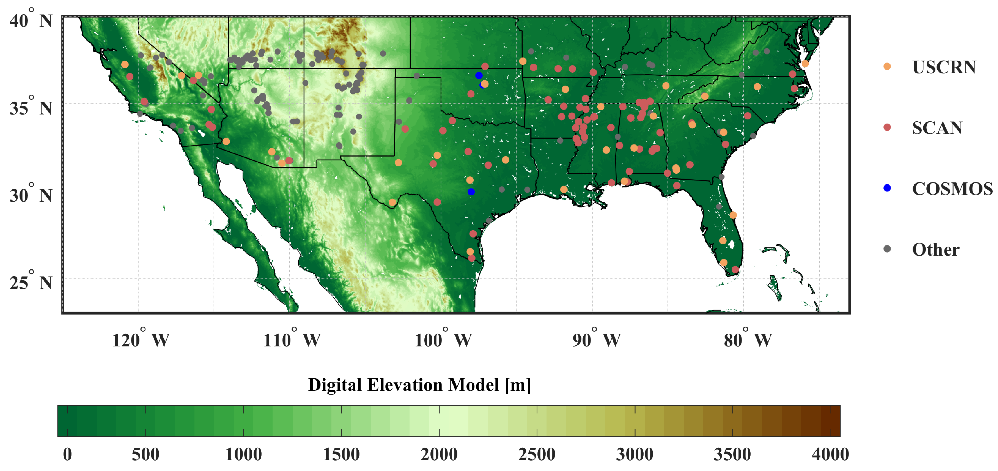
The aforementioned CYGNSS observables need to be accompanied with several auxiliary land surface parameters to describe the interaction of received signals with the land surface. To construct the nonlinear relationship between CYGNSS observations and these parameters including SM information through ML approaches, labeled in-situ SM measurements are needed. The in-situ SM data available at the ISMN sites [25] are used as the reference data and are assumed to be representative over a 9 km × 9 km grid cell [18]. The ISMN has assembled over 50 operational and experimental SM networks worldwide, providing a global in-situ SM database with uniform data format and pre-processing quality flags [26]. While there are some sites in Asia, Australia and Europe, sites that provide both temporally and spatially collocated observations with regards to CYGNSS data are mainly in North America. In this study, we consider all available sites over CONUS within the CYGNSS spatial coverage (shown in Figure 1). Detailed information about the ISMN is reported in [25,27]. The ISMN dataset is publicly accessible (http://ismn.geo.tuwien.ac.at).
The hourly SM data from ISMN are masked using the provided quality flag (identified as ‘good’ with ‘G’) and then averaged to daily values. The surface SM at 5 cm depth is used which is consistent with the penetration depth of L-band microwave signals. In total, there are more than 200 ISMN sites with ground-based observations between March 2017 and December 2019 within the CYGNSS spatial coverage in CONUS. These sites are mainly from the Soil Climate Analysis Network (SCAN), U.S. Climate Reference Network (USCRN), and the COsmic-ray Soil Moisture Observing System (COSMOS). Since many effects including complex topography and surface open water can significantly affect CYGNSS received observations, a detailed masking criteria is applied to all ISMN sites as described in Section 2.4. Quality control masks and the number of ISMN for each utilized network is provided in Table 1.
2.3. Ancillary Data
Received GNSS-R signals are affected by various land surface characteristics such as land cover, topography, water bodies, and soil texture in addition to the SM value as stated previously. To account for the impact of land surface characteristics, various time-varying or static physical remote sensing-based land surface parameters are utilized as features in the ML framework. The spatial resolution of CYGNSS observations (that dictates the spatial extent of the ancillary data) is linked to the nature of the scattering surface. It is determined by the first Fresnel zone (several kilometers) in the case of specular (coherent) scattering, and by the glistening zone (several tens of kilometers) in the case of the non-specular (diffuse) scattering. In this study, a coherent reflection is assumed, which is valid when the contributing area is relatively flat and smooth ground with no or light vegetation cover. The “effective size” of the first Fresnel zone is highly variable, and depends on the ranges from specular point to the transmitter and the receiver, specular reflection angle, and operating frequency. It also gets smeared along the track depending on the coherent integration time of the receiver. For most applications, the CYGNSS data is usually gridded to regular grid cells with a fixed resolution under the coherent assumption [13,15]. In our previous work [18], we considered an approximate 4 km × 4 km grid cell that centered the specular point to generate the mean terrain characteristics. Here, the spatial resolution of CYGNSS data is assumed to be 3 km × 3 km which leads to the optimal results from several tests under different spatial resolution assumptions in our pre-test experiments. Therefore, the auxiliary land surface characteristics are spatially aggregated from their native resolutions to 3 km. For CYGNSS specular points located within the 9 km grid centered at each ISMN site, the reference labels are assumed to be the same for one particular day. Each specular point has its own auxiliary data from a 3 km grid centered at the specular point, including physical parameters of DEM elevation, slope, NDVI, and soil texture.
The 500 m resolution, 16-day composite NDVI from MODIS (MYD13A1) is utilized for characterizing the spatio-temporal variations of vegetation conditions. To be consistent with the assumed spatial resolution of CYGNSS data, MODIS NDVI data has been spatially averaged from its original 500 m to 3 km for grids centered at specular points. The MYD13A1 dataset can be acquired from the NASA Land Processes Distributed Active Archive Center (https://lpdaac.usgs.gov/products/myd13a1v006/).
A dominant land cover type map at 500 m resolution is also obtained from the MODIS yearly Land Cover Type (MCD12Q1) product in 2018. This product provides the dominant land cover type for each grid cell. Six classification schemes are included, and the primary International Geosphere Biosphere Programme (IGBP) land cover scheme is selected for further analysis. IGBP contains 17 land cover classes, including water, forest, shrublands, grasslands, cultivated land, wetlands, artificial surfaces, permanent snow and ice, and bareland. For each 3 km grid, the most frequent land cover type is determined. In addition, the land cover information is used to calculate Vegetation Water Content (VWC) and surface roughness (H-value) parameters using the same lookup tables as in the SMAP product [28]. Specifically, both VWC and H-values are obtained using the weighted averages of the lookup table values with weights determined by the percentages of corresponding land cover types within each 3 km grid cell.
The topographic information, known to greatly affect the reflectivity of GNSS-R signals [29], is derived from the 1 km Digital Elevation Model GTOPO30 product. This can be obtained from the United States Geological Survey Earth Resources Observation and Science archive (doi: /10.5066/F7DF6PQS). Elevation and slope are calculated and aggregated from 1 km to 3 km. Similar to other datasets, the spatial regridding for topography is conducted for each 3 km grid centered at the specular point and averages of elevation and slope are used to represent the underlying topographic complexities.
The presence of surface inland water body is identified by utilizing a 30 m Global Surface Water Dataset from the Joint Research Centre (GSW-JRC) [30]. Particularly, the seasonality map in 2018 provides the intra-annual behavior of surface water and the number of months where permanent or seasonal surface water were present. These 30 m seasonality maps are aggregated to 3 km for representing the percentages of surface inland water within the CYGNSS observed reflection area. The water percent is determined by calculating the percentage of 30 m grids within each 3 km grid indicating the presence of either permanent or seasonal water, and this value is used during the retrieval algorithm’s quality control phase.
The Global Gridded Soil Information (SoilGrids) [31] is used to represent soil texture that controls hydraulic properties such as water retention and capillary action within the profile. In SoilGrids, the soil profile is vertically discretized to seven layers with a maximum depth of 2 m. For each layer, the soil is classified into 12 standard soil texture classes based on the sand, clay, and silt proportions. Here, the 5 cm depth is used for consistency with the penetration depth of L-band signals. The product is available at 250 m and spatially aggregated to 3 km for each specular point. Sand, clay, and silt proportions are spatially averaged, and the dominant soil texture class is determined by the percentages of the 12 soil texture classes.
2.4. Quality Control Mechanisms
In total, there are over 160,000 CYGNSS observations available from March 2017 to December 2019 over ISMN sites in CONUS. However, critical screening for the quality of CYGNSS observations and underlying land surface conditions is needed before conducting SM retrieval. Several filtering criteria for quality control are applied to CYGNSS observations, ancillary data, and in-situ SM measurements.
CYGNSS metadata contains many quality control flags for both the raw instrument data and processing information. Thus, observations with relatively low quality can be easily removed by quality flags that indicate a potentially unreliable GNSS-R observation. In the study, we use the specific flags (S-band powered up, large spacecraft attitude error, black-body DDM, DDM test pattern, low confidence GPS EIRP estimate) and methods reported in [13,15]. Additionally, CYGNSS observations with a negative antenna gain are filtered from the input dataset. Observations with an incidence angle higher than 65° [14] are removed to avoid the inclusion of noisy DDMs. Also, observations with a DDM peak value outside of 5 to 11 delay bins are removed from the dataset to avoid the inclusion of high-altitude measurements [13].
Open water near the specular point is a critical error source for SM retrieval products. The power of a forward-scattered signal emanating from a water’s surface is generally several orders of magnitude higher than a signal scattered from soil due to the very strong coherency over water surfaces [32]. The SM retrieval near water bodies, thus, becomes infeasible if the surface water is sufficiently large within the CYGNSS footprint. Hence, a CYGNSS observation is excluded if more than two percent of the 3 km grid centered on a specular point is covered with permanent or seasonal water.
In addition, CYGNSS observations that fall over forested regions with VWC > 5 kg/m2 (dense vegetation canopy) [33] and with a dominant urban land cover type [34] are filtered and removed using the land cover type data described in Section 2.3. Furthermore, CYGNSS observations, which corresponds to a total of 84 ISMN sites in the CONUS, are also masked out due to a limited elevation algorithm at the first stage of CYGNSS mission.
Table 1 summarizes some information about the raw dataset, quality mechanisms, and their ratios on the raw dataset and filtered dataset statistics. From 2017 to 2019, there are 234 sites over CONUS reporting SM data from COSMOS, SCAN, and USCRN networks. The concurrent number of data samples from CYGNSS and ISMN is . After applying specified quality control criteria, total of 106 sites with concurrent CYGNSS observations for SM retrieval is achieved.
3. Methodology
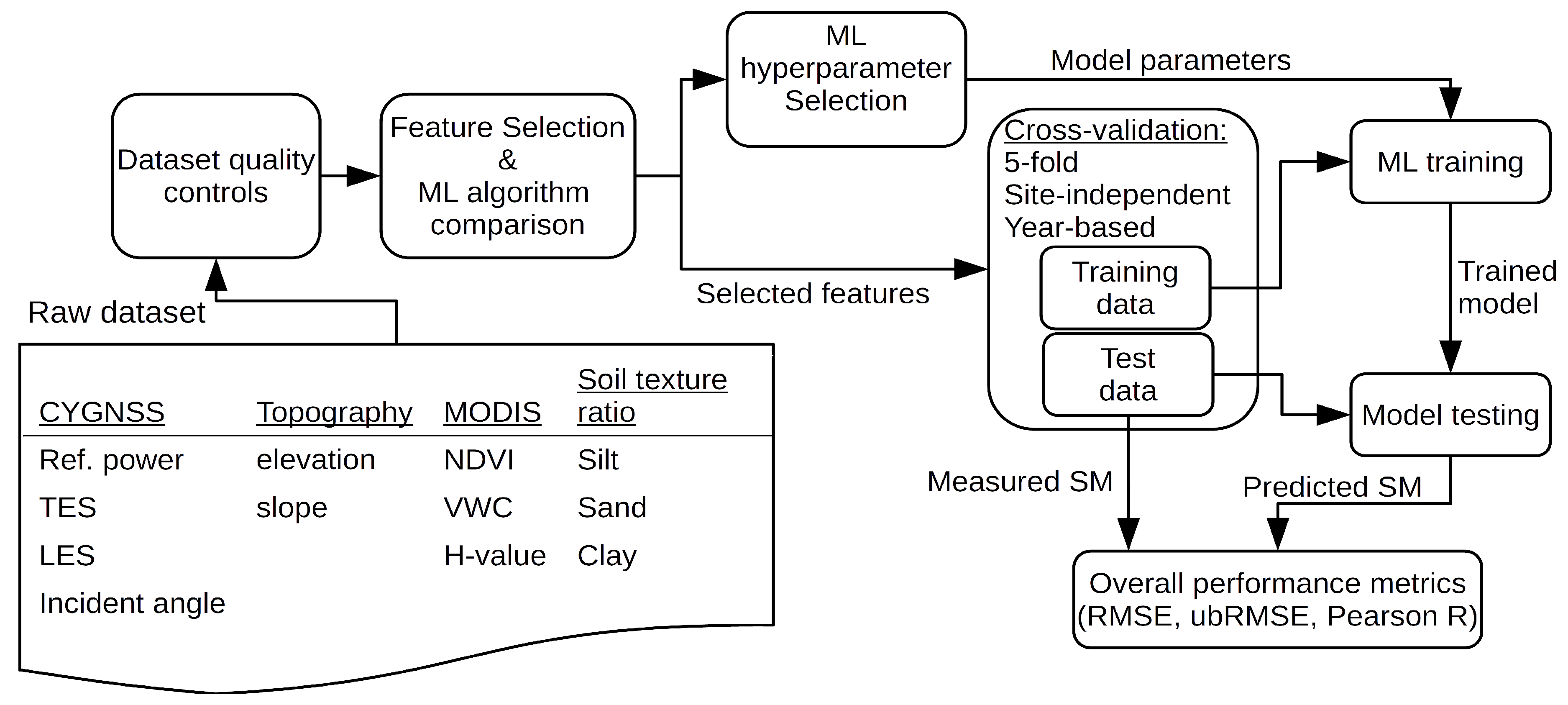
The accuracy of SM estimation retrieved from GNSS-R observations is dependent on a proper modeling of the complex and nonlinear relationship between the forward-scattered signal and environmental variables such as system geometry, surface roughness, topography, and soil properties. It is highly complex to model all such interactions with high fidelity. Instead, our methodology uses data-driven ML approaches with physics-based features that have direct, physical relations to SM estimation. Since ML algorithms are excellent function approximators and have a remarkable capability in modeling complex and nonlinear relationships, ML is a well-suited approach for the CYGNSS-based SM retrieval problem. All available ISMN sites over CONUS are utilized to conduct extensive analysis on both the ML approaches and their performance dependence on utilized physical features. The overall SM retrieval algorithm used in this study is depicted in Figure 2 and briefly summarized in Section 3.3.
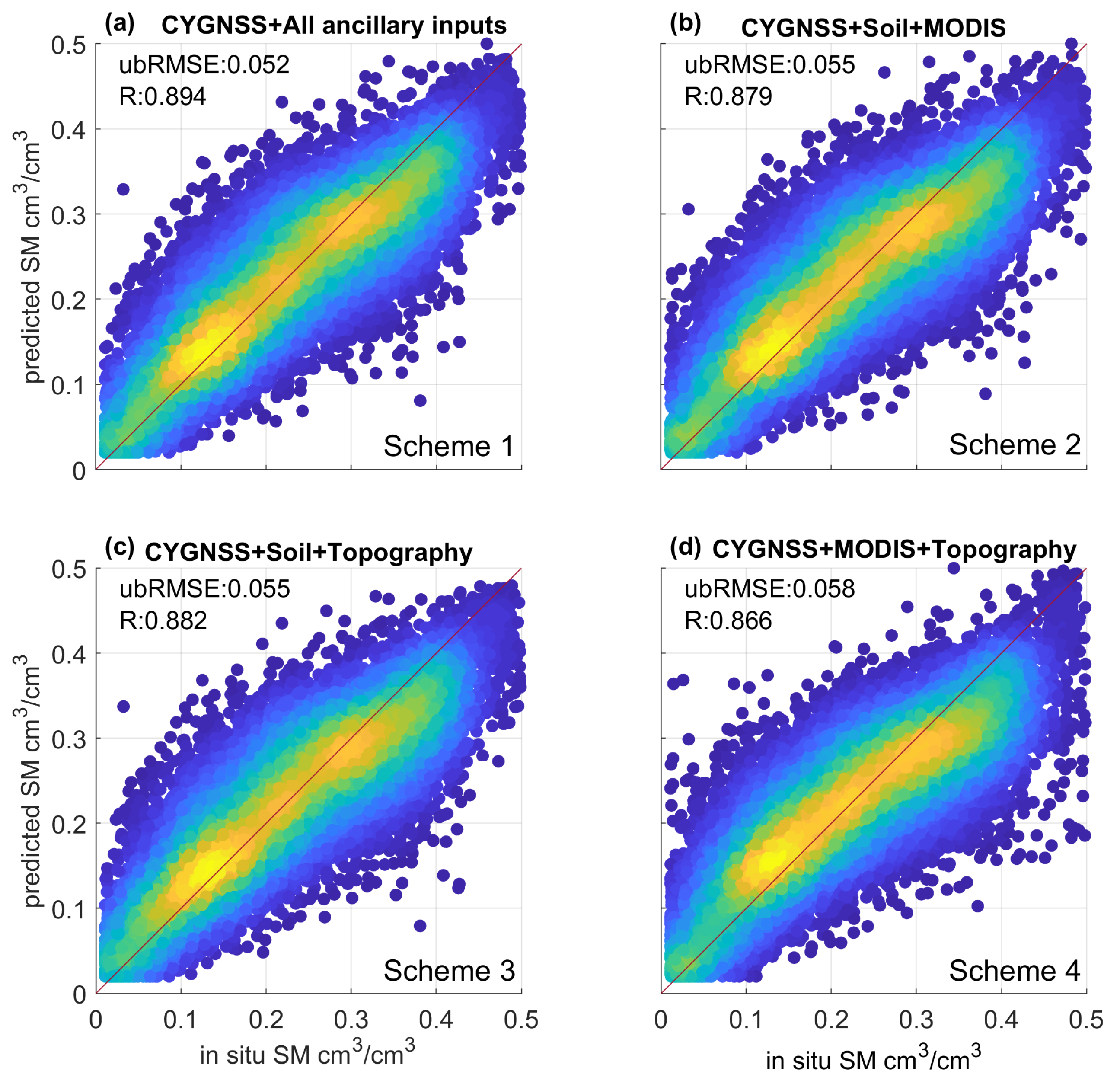
In this study, a supervised learning problem is considered that maps the inputs, which are physical features related to land scattering characteristics, to the labels, which are the measured SM values at ISMN sites. CYGNSS and the ancillary dataset that form the input features for the proposed supervised learning approach are presented in Section 2 along with the preprocessing and quality control mechanisms. The physical features for CYGNSS-based SM retrieval are separated into four main groups: CYGNSS observables, topography, MODIS, and soil texture features. All of the 12 physical features in these groups are listed and described in Table 2. To interpret the effect of different types of ancillary data, different ML models are trained and validated by excluding one ancillary input group at a time. Therefore, four different schemes of input feature groups are constructed as below and discussed in Section 4.1.
Scheme 1: default scheme with + CYGNSS.
Scheme 2: + CYGNSS.
Scheme 3: + CYGNSS.
Scheme 4: + CYGNSS.
In the following subsections, we describe in detail the trade-offs in use of different ML-algorithms, determination of optimum hyperparameters of the algorithms, selecting most relevant features as well as strategies to evaluate the performance of the framework.
3.1. Machine Learning Algorithm and Feature Selection
The selection of a ML algorithm and its hyperparameters that are most suitable for the SM retrieval problem is a critical decision and has a significant impact on the performance of SM prediction. We compare ANN, Random Forest (RF), and Support Vector Machine (SVM) approaches, which are popularly used for supervised regression problems.
ANN is one of the most common ML algorithms for nonparametric and nonlinear classification or regression problems [35]. ANNs are networks formed by interconnections between neurons with nonlinear activations. Each neuron is a model that receives a linearly weighted combination of outputs from previous layers and outputs a result passing that linear combination through its nonlinear activation function. A feed-forward ANN of a multi-layer perceptron structure is usually composed of an input layer, one or more hidden layers, and an output layer. The total number of layers and number of nodes used in each hidden layer determines the total number of weights that must be learned through minimizing the total cost between ANN predictions and the actual measured outputs in the training data.
SVM is a supervised nonparametric learning method [36]. The basic idea of the SVM is to find hyperplanes that separates training samples into a predefined number of classes. SVM can also be applied to nonlinearly separable problems by using a kernel function [37]. The accuracy of SVM depends on the hyperparameters of the error penalty parameter and the parameters of kernel functions. These two critical parameters need to be optimized if a radial basis function (RBF) is selected.
RF is an ensemble ML algorithm that forms multiple decision trees. Each decision tree contains a root node, internal nodes, and leaf nodes. In the forest, each decision tree makes its prediction, and then the mean prediction of the trees is calculated as the output of the RF for a regression problem [38]. The important hyperparameter defining the RF performance is the number of decision trees utilized in the RF algorithm.
Hyperparameters are model parameters specified before the learning process. Typical hyperparameters include the number of hidden layers and neurons in ANN, the regularization coefficients and parameters in the kernel function of SVM, maximum split size, and the size of the ensemble tree in RF algorithms, etc. The selection of hyperparameters mainly determines the ML model and thus has a critical impact on SM prediction performance. Optimal hyperparameters should be used to prevent overfitting and underfitting of the ML technique to the training dataset. The optimal operating points of each ML model are obtained by utilizing a grid search method for their hyperparameters as presented in Section 4.1.
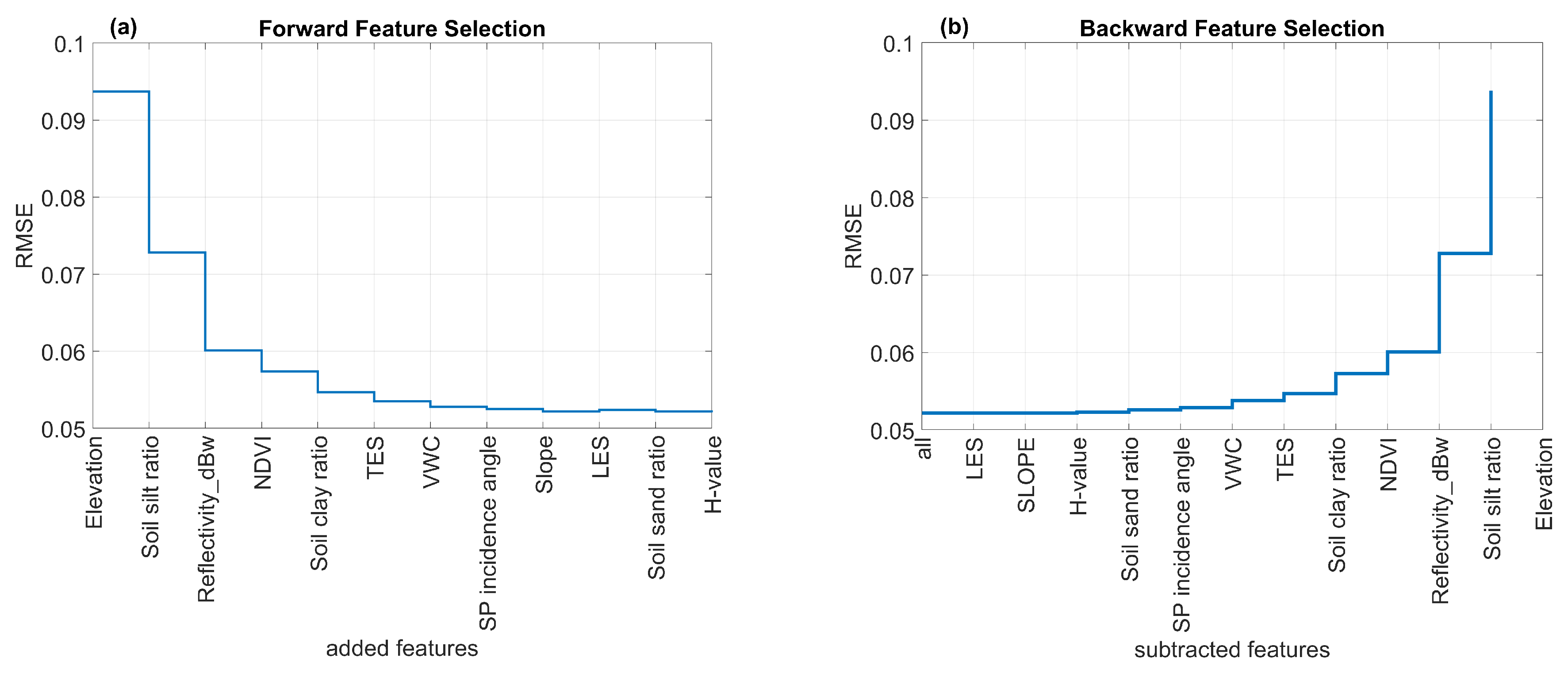
Initially, 12 features from CYGNSS, MODIS, soil texture and topography feature groups are used (Table 2). However, using too many features or too complex models may lead to an overfitting with the ML model. A large feature set can contain noisy features or cross-correlated features that might lead to marginal improvements or even deteriorations in final performance. Moreover, using too many features will increase the computational cost. Thus, it is highly essential to select a subset of relevant features. In this work, the sequential feature selection, forward or backward, algorithms are used to choose the most relevant feature subset. The sequential feature selection is widely used for its simplicity and speed in many applications [39,40]. Forward sequential feature selection is an iterative technique that selects at each iteration the subset of features that minimizes the defined cost function. Starting with the best-performing single feature and sequentially adding the next best feature, the iteration continues until a certain stopping criterion is satisfied or all features are used. In the backward feature selection method, the algorithm removes one less significant feature at a time. This process is repeated until there is no feature to be removed or when a stopping criterion is reached. The feature selection results are described in Section 4.1.
3.2. Performance Metrics and Evaluation
Results are evaluated in terms of the root-mean-square error (RMSE), unbiased RMSE (ubRMSE), bias, and correlation coefficient (R) between the predicted SM values and the measured SM from in-situ sites. To evaluate how well the performance of the proposed method could be generalized, three different cross-validation techniques are deployed: (1) 5-fold, (2) site-independent, and (3) year-based.
For a 5-fold cross-validation, the data set is first split into 5 folds, then 4 folds are used as the training set, and the remaining fold is used as the testing set. The final evaluation result is the averaged result of each fold. To evaluate the capability of the prediction model to be generalized, a site-independent cross-validation approach is also tested. In this approach, data for a single SM site is used as test dataset while data for all other SM sites are used in training. By this way, the prediction performance of ML for a totally unseen site can be analyzed. The RMSE, ubRMSE, bias, and R values are computed separately for each site under this validation case. For a year-based cross-validation method, the proposed model is first trained with data from 2017 and 2018 and then tested on data from the year 2019. This year-based validation process is repeated for each combination of the three observation years. As seen in Table 1, the number of observations of each year is different. Hence, it should be noticed that the contribution of years to the training model would not be similar.
3.3. Machine Learning Framework Summary
Figure 1 encapsulates the following, overall workflow of the ML-based SM product. The raw dataset which contains CYGNSS-based reflectivity and geometry, MODIS-based vegetation information, GTOPO30-based topography information, and SoilGrid-based soil texture data are compiled into a single dataset for analysis. These individual datasets are described in detail within Section 2.1 and Section 2.3. Data that contain potentially unreliable information are filtered out using the dataset quality control processes described in Section 2.4. The optimal hyperparameters for ML methods are chosen as discussed in Section 3.1. Redundant input features are then eliminated using the feature selection process described in Section 3.1. Using a portion of the ISMN data described in Section 2.2 as reference labels, the selected ML method is trained with the filtered input dataset. The remaining portion of ISMN data is considered a testing dataset and is used for model testing. The metrics for this model testing are defined in Section 3.2. Finally, this entire process is performed for different input dataset schemes as defined in Section 3. All analyses and model development processes are performed using the machine learning toolbox of MATLAB R2019b software.
4. Results
In this section, the SM retrieval results from varying ML-based approaches are presented from four perspectives. In Section 4.1, the performance of different ML algorithms and input features are first explored. With the selected ML technique and input features, the overall performance of the ML model for SM retrieval is evaluated in Section 4.2 through three cross-validation strategies (as described in Section 3.2). The spatial distribution of the ML-based SM retrieval performance is also presented in this part. Section 4.3 analyzes the effect of different land cover types and soil texture conditions on the SM prediction performance via a 5-fold cross validation method. In addition, the impact of different in-situ SM networks on the performance is examined. In Section 4.4, two representative ISMN sites are selected and their performance are demonstrated in the temporal domain.
4.1. Examination of Different Machine Learning Algorithms and Input Features
As stated in Section 3.1, hyperparameters and, hence, the ML-based model itself require careful selection in order to prevent overfitting or underfitting. Here, we first analyze the ML algorithm performance with a varying set of model parameters with 5-fold cross-validation. The selected grid search ranges for hyperparameters are the number of trees (from 10 to 1250 with a 10-step interval) and maximum split size (from 1 to 250 with a 5-step interval) for RF, hidden neuron size (from 5 to 100 with a 5-step interval) and layer size (from 1 to 3) for ANN, kernel scale (from to ) and penalty parameter (from to ) for SVM. During the grid search process, the model complexity is determined in terms of total weight number for ANN and total nodes number for RF. In ANN, the number of weights is a function of the number of features, the number of layers, and the number of neurons. For an RF model, the total number of nodes is the sum of the number of nodes of each decision tree. For SVM, the number of features and kernel scale are the main parameters that affect the model complexity.
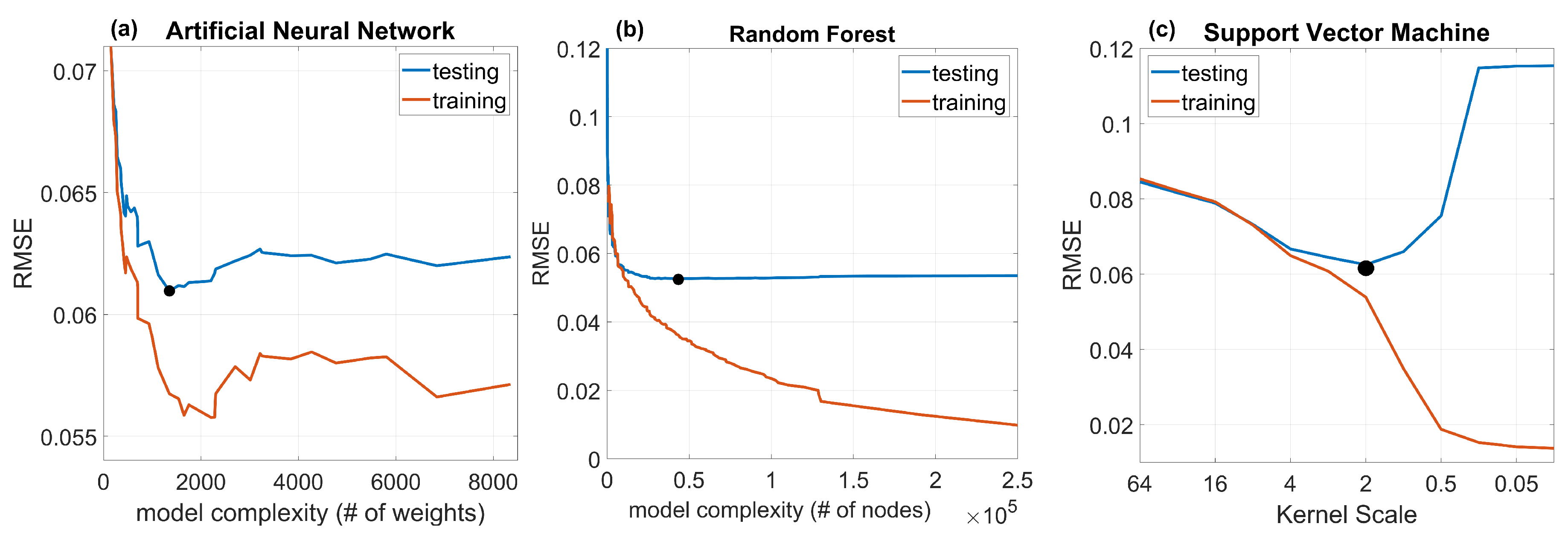
Figure 3 shows the validation curves for each evaluated ML approach. The training and validation RMSE curves are shown as a function of the varying model parameters obtained from the grid search process for each ML algorithm. The black circle as shown on each ML approach’s validation curve indicates the optimal model order and hyperparameter selection that generates the minimum RMSE on the testing dataset. It is clear and expected that the RMSE of the training dataset generally decreases with increasing model complexity for all compared ML algorithms. However, exclusively minimizing the RMSE value for the training dataset can produce overfitting if the RMSE of the testing dataset is not considered during hyperparameter selection. For ANN, a minimum RMSE value of 0.061 cm/cm on the testing dataset is obtained with three layers and 25 hidden neurons for each hidden layer (Figure 3a). For RF the minimum testing dataset RMSE of 0.052 cm/cm can be obtained with 120 maximum split size and 200 trees (Figure 3b). Similarly, the optimal penalty parameter and kernel scale of SVM are obtained as one and two, respectively, with a minimum RMSE of 0.065 cm/cm (Figure 3c). Comparing the three ML algorithms, RF delivers the smallest RMSE value on the testing dataset. Therefore, the RF is chosen as the ML algorithm for SM retrieval in this work and is used in subsequent analysis.
To understand the impact of the four raw input datasets depicted in Table 2 on the total RMSE, four schemes with different combinations of input feature groups (specified in Section 3) are analyzed using the RF regression model and a 5-fold cross-validation method. Note that the initial 12 features are separated into four groups and are fully included in the Scheme 1 as a benchmark for evaluating the effect of each independent ancillary feature group. Figure 4 shows predicted SM values compared against in-situ observations for four different schemes. For the case with all 12 features as input data, a minimum ubRMSE of 0.052 cm/cm and a maximum R of 0.894 [-] is obtained via a 5-fold cross-validation method (Figure 4a). For cases where one of the three ancillary feature groups is excluded from the input data, e.g., the topography information is excluded in Figure 4b, the ubRMSE/R values are changed from 0.052 cm/cm/0.894 [-] to 0.055 cm/cm/0.879 [-] when comparing the ML model predicted SM and in-situ data. Likewise, the removal of either MODIS (Figure 4c) or soil information (Figure 4d) leads to degraded model performance. Particularly, soil texture features are identified as the most influential ancillary input for the SM prediction with a net ubRMSE increase of 0.006 cm/cm in Scheme 4. Both MODIS features (i.e., NDVI, VWC, and H-value) and topography features (elevation and slope) are critical for predicting SM as indicated in Figure 4b,c. In combination, the MODIS, topography, and soil texture feature groups provide complementary information of underlying land surface conditions with respect to CYGNSS observables and therefore are necessary for accurate SM retrieval in the ML modeling process.
However, within each feature group, there exists repetitive and cross-correlated information that can slow down the ML modeling process and introduce irrelevant noises. To reduce the input feature size without reducing the retrieval accuracy, the sequential feature selection is conducted. Figure 5 shows the forward and backward sequential feature selection results via a 5-fold cross-validation method. For either forward or backward feature selection, a minimum RMSE of 0.052 cm/cm is achieved with eight input features. Further inclusion of new features, i.e., soil sand ratio, H-value, slope, and LES, does not introduce any significant improvements to the regression performance (Figure 5a,b). Thus, an optimal feature number of 8 is determined for the rest of this study. The eight most relevant input features used for SM retrieval are elevation, soil silt and clay ratios, NDVI, VWC, reflectivity, TES, and SP incidence angle (see Table 2 for full descriptions).
4.2. Overall Performance of the Machine Learning Retrieval Model
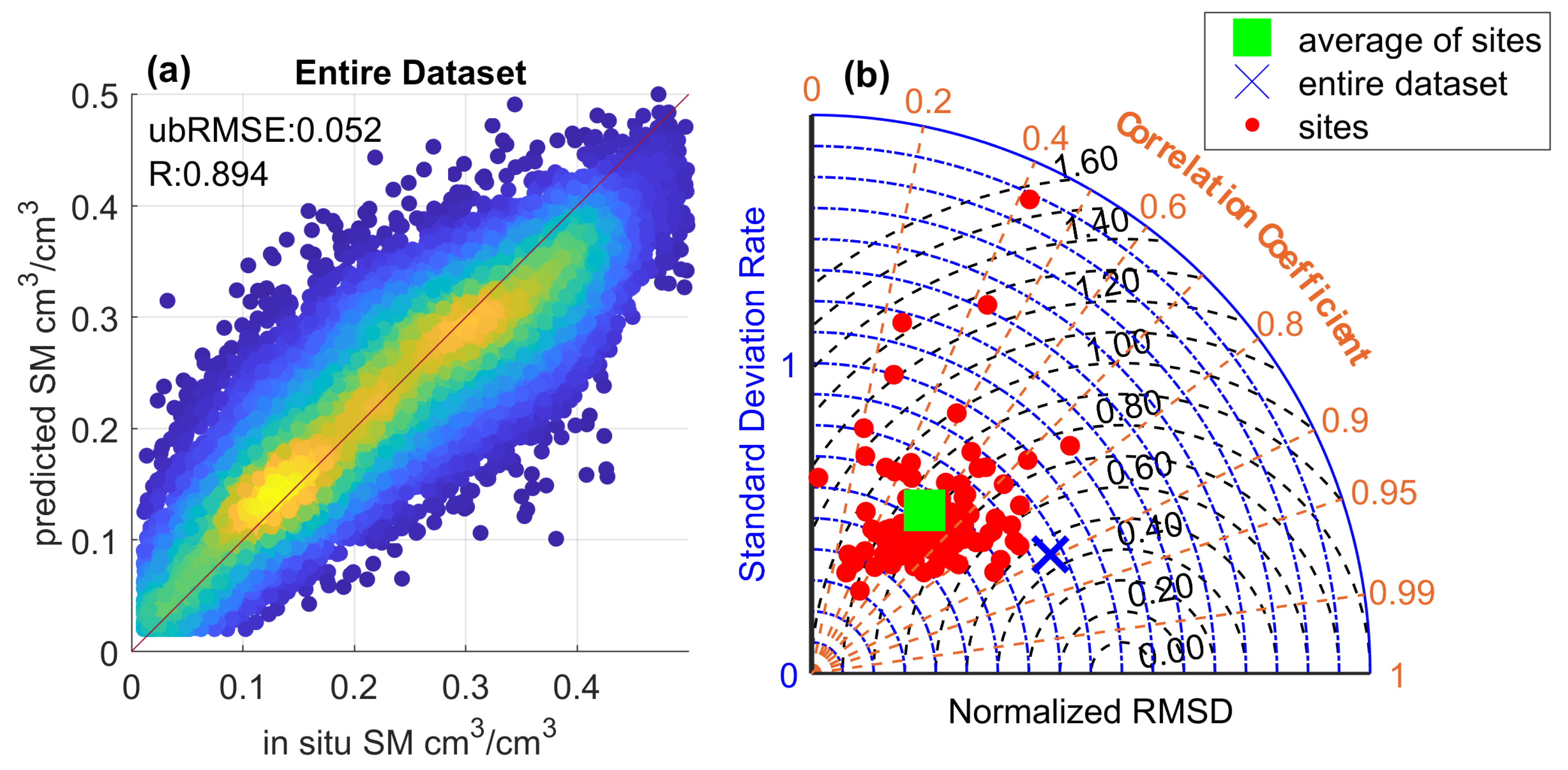
Figure 6 and Table 3 show the overall SM prediction performance derived via the RF regression model with eight input features. The RF method in a 5-fold cross-validation approach reaches an overall ubRMSE of 0.052 cm/cm and a R value of 0.894 [-] over the whole dataset. For all 106 ISMN sites, the mean ubRMSE is obtained as 0.047 cm/cm with a standard deviation of 0.016 cm/cm whereas the best and poorest scores are 0.09 and 0.085 cm/cm, respectively. The averaged absolute biases across sites is 0.011 cm/cm with a standard deviation of 0.013 cm/cm (Table 3). Note that different ISMN sites can show distinct SM climatology, leading to the prediction biases through the ML model with incomplete sampling space. For the 5-fold cross-validation method, 80% of the whole dataset is sampled randomly for use as a training dataset and the ML-based prediction model is tested on the remaining 20% of the data. The biases suggest that the ML model is dependent on the representativeness of the sampling set.
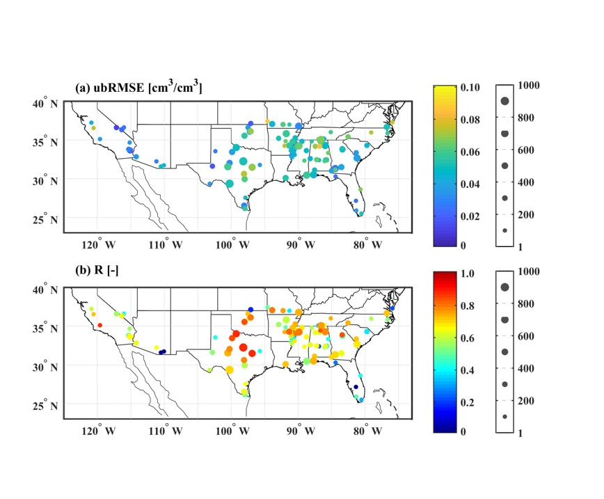
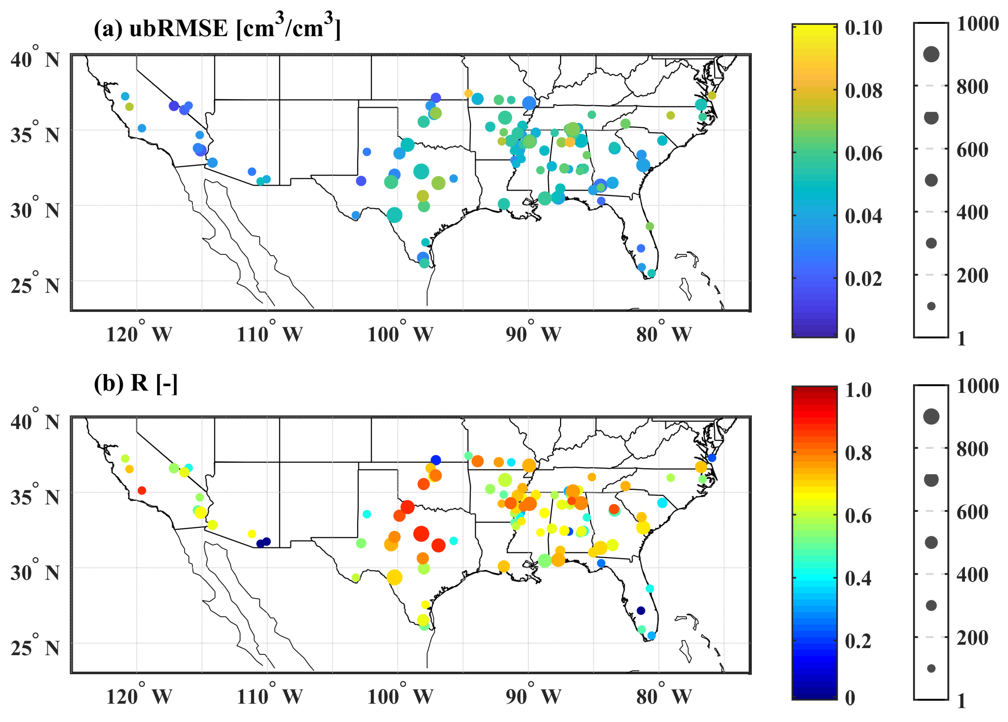
Figure 7 shows the spatial distribution and variations of the RF-based SM retrieval model across the CONUS sites. A satisfactory performance is achieved with ubRMSE smaller than 0.045 cm/cm (Figure 7a) and R larger than 0.7 [-] (Figure 7b) for the majority of sites. Sites with small R values generally correspond to those with relatively few concurrent in-situ observations and CYGNSS data (the number of concurrent samples is less than 100) as shown in Figure 7b. Overall, the 5-fold cross-validation results indicate that the RF-based SM retrieval model is capable of generating satisfactory SM estimates.
In addition to the 5-fold cross-validation, a site-independent cross-validation, or the “leave-one-subject-out” method, is applied which depicts the most challenging strategy to determine how well the proposed method generalizes for new sites’ observations that are totally unseen during the training process. For this purpose, the RF model is trained over 105 sites and tested on all observations at the unseen site. This validation procedure is conducted independently for 106 sites. The overall performance statistics across 106 sites in the site-independent cross-validation are provided in Table 3. The mean ubRMSE of all sites is relatively low with a value of 0.054 cm/cm indicating that the RF-based SM prediction model can predict the temporal variations of SM for new site or unseen regions. However, relatively large RMSE (0.084 cm/cm) and mean absolute bias (0.056 cm/cm) across sites suggest that the ML-based prediction model is less capable of dealing with systematic bias issues. As noted above, different sites can have distinct climatology that can be difficult for the ML model to capture if no a priori information is provided. In this site-independent cross-validation method, this phenomenon is further exaggerated since no information will be available for the learning process over the unseen site. Increasing the spatial coverage of the training dataset with more complete characterization of various land surface conditions can potentially improve the performance of ML-based SM retrieval model. However, with limited in-situ sites, increasing the spatial representativeness of the training data will require a global satellite-based SM data which is beyond the scope of this work.
Moreover, in order to test the ML-based model for predicting SM estimation under yearly temporal variations, the model is first trained on the data from 2017 and 2018 and then tested on the data from 2019. This cross-validation process is referred as year-based validation and has been repeated for 2017 and 2018. The performance metrics are shown in Table 3 for each testing year. The ubRMSE values for 2017, 2018, and 2019 in the year-based validation are 0.048, 0.047, and 0.050 cm/cm, respectively. The relatively low ubRMSE values suggest that the ML-based prediction model can be applied to new observations. In the year-based validation, each site provides partial time series data for the training, and the corresponding ML-based model contains a certain amount of the site-specific information for SM retrieval. The low absolute bias error and RMSE, as compared to the site-independent validation, further indicates the importance of a priori information on the prediction capability of the ML-based model. The smaller RMSE scores for 2017 and 2018 testing years can be primarily traced back to the number of observation. For year 2019, the ML model is trained with a relatively small dataset and tested on a large dataset.
4.3. Effect of Underlying Land Surface Conditions
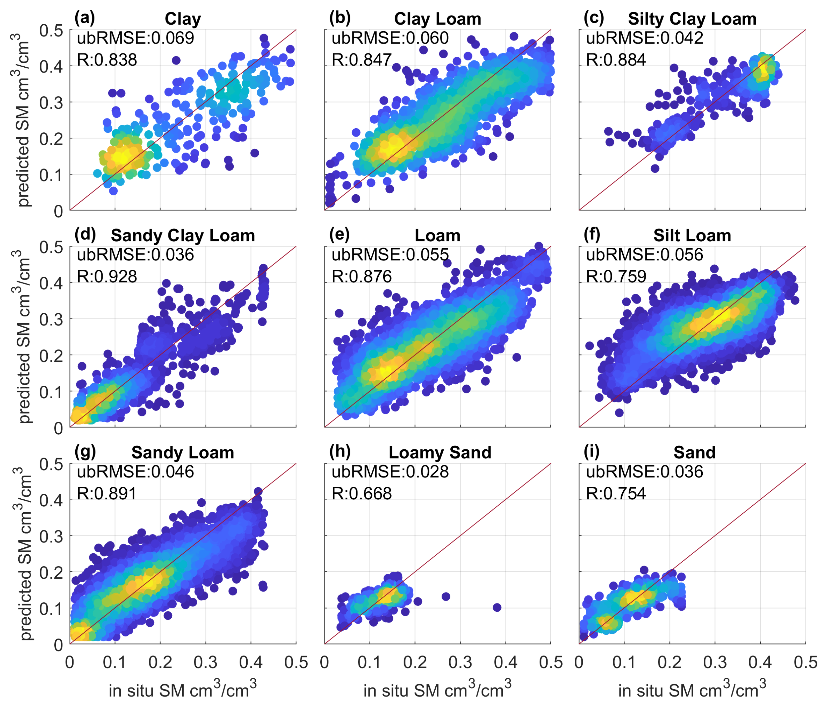
To evaluate the overall prediction performance of the ML-based SM retrieval model, it is also important to quantify the impact of different land surface conditions since factors such as soil texture are known to be critical parameters that affect both GNSS-R measurements and retrieval performance. In Figure 8, the SM predictions are compared to in-situ SM under 12 main soil texture classes. As demonstrated, the predicted and observed SM estimates are generally well aligned with the 1:1 line. For clay and clay loam classes, the observed SM changes from a minimum of 0.01 cm/cm to a maximum of 0.5 cm/cm with large variations. The predicted SM estimates have ubRMSE values greater than 0.06 cm/cm as compared to ISMN observations. Particularly for clay (Figure 8a), the SM data are concentrated with either high or low values. Moreover, the sampling size of clay is relatively small which further impedes the ML process. On the contrary, the SM is consistently high/low for silty clay loam/sandy clay loam, leading to smaller ubRMSE of 0.042/0.036 cm/cm and higher R of 0.884/0.928 [-]. For loam, silt loam, and sandy loam, the SM observations are more evenly distributed as shown in Figure 8e,f,g. The ubRMSE values for these three soil texture classes are around 0.050 cm/cm and R values are generally high. As shown in Figure 8h,i, the observed SM values are generally below 0.20 cm/cm and thus relatively small ubRMSE values (0.028 and 0.036 cm/cm ) are as expected.
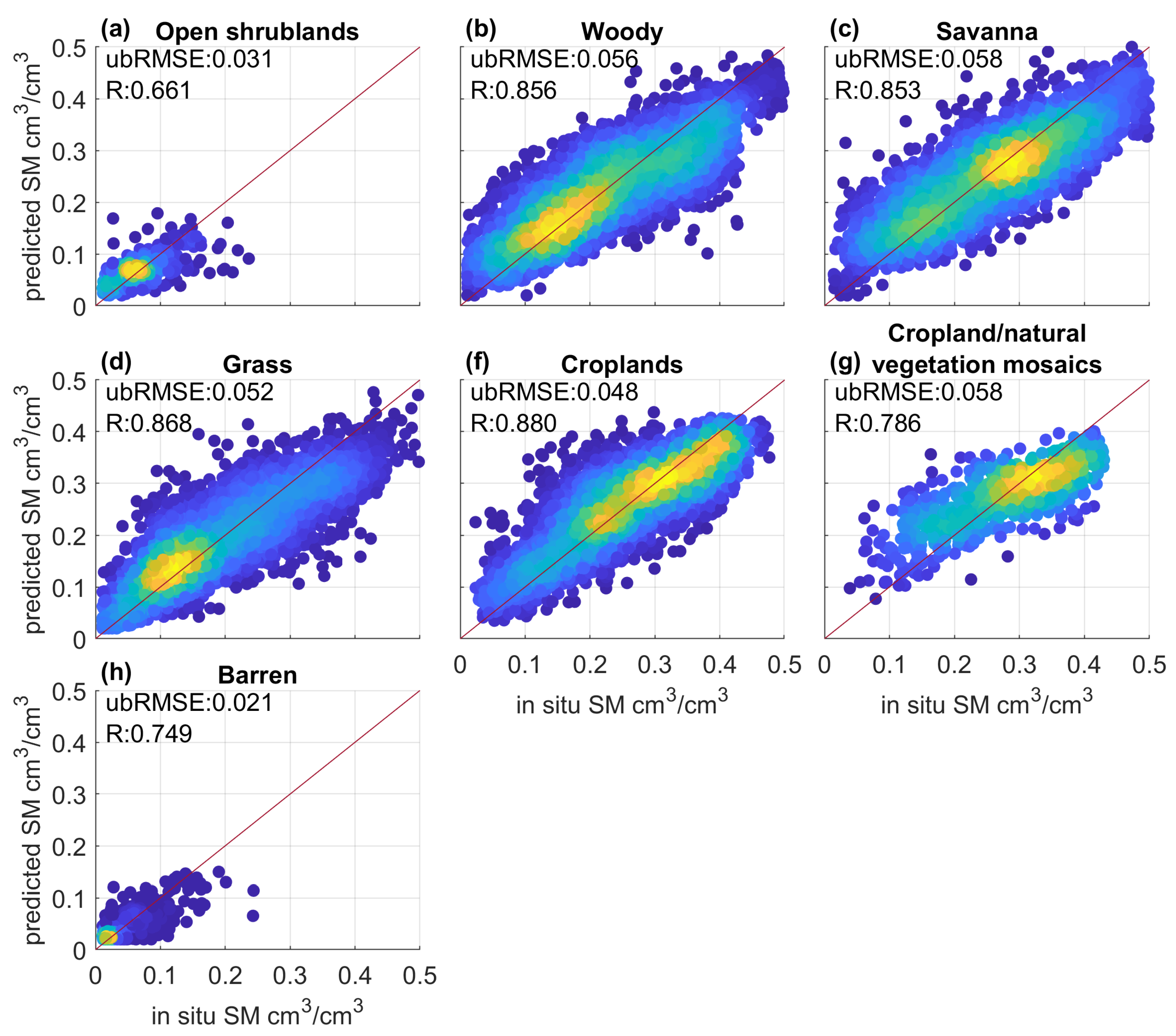
Furthermore, the ML-based model prediction capabilities for different land cover types are analyzed and shown in Figure 9. In total, there are eight primary land cover types that are examined. Regions with open shrublands (Figure 9a) and barren (Figure 9h) land cover are generally associated with relatively dry soil at the ISMN sites. Thus, the ubRMSE values are relatively small (0.031 and 0.021 cm/cm) and correlations tend to be comparatively low (0.661 and 0.749 [-]). For other land cover types, i.e., woody (Figure 9b), savanna (Figure 9c), grass (Figure 9d), croplands (Figure 9f), the observed SM varies from a minimum of 0.01 cm/cm to a maximum of 0.50 cm/cm. In addition, the sampling sizes for these four land cover types are comparably large which benefit a ML-based model to capture the empirical relationship between input features and reference data. The achieved ubRMSE and R values are around 0.050 cm/cm and over 0.85 [-] respectively. The relatively small sampling size may be the main reason for a low R (0.786 [-]) over cropland with natural vegetation mosaics land cover type (Figure 9g).
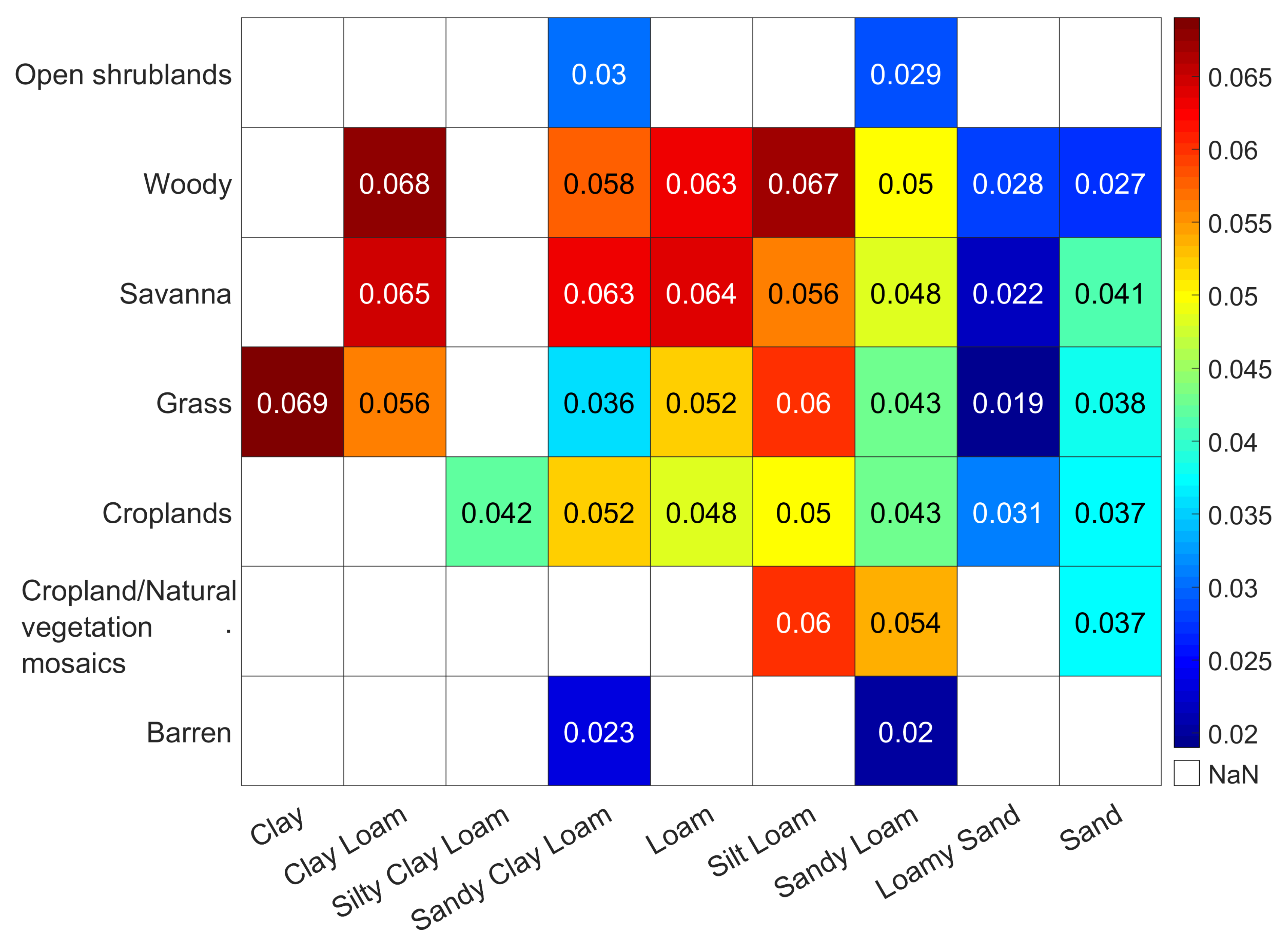
When synergistically considering the land cover type and soil texture class, the prediction performance of the ML-based model is shown in Figure 10. As described above, the ubRMSE values are generally small for open shrublands, barren, loamy sand, and sand types. For cases where the dominant soil texture is sandy loam, the ubRMSE scores for different land cover types are mostly below 0.05 cm/cm except for cropland/natural vegetation mosaics. More importantly, the predicted SM estimates generally have consistently high accuracy (with ubRMSE less than 0.05 cm/cm) for croplands under different soil texture classes. The accurate soil water monitoring over croplands is important, and hence, the prediction capability demonstrated here suggests that the ML-based retrieval model can be utilized for agricultural soil water monitoring using the CYGNSS data.
The preceding analysis makes use of the entire ISMN dataset using the RF algorithm with eight selected input features. It is important to note that the in-situ SM observations are collected using different ground-based sensors with distinct set-up environments for the three examined observation networks. It is advisable to investigate the impact of the different in-situ SM networks on the performance of the learned ML model. To this end, three different RF-based regression models are learned with datasets from the three in-situ SM networks separately, i.e., COSMOS, SCAN, USCRN. The 5-fold cross-validation results are shown in Figure 11 and Table 4 for each network-based ML model. By training and testing the ML model with SM observations that are separated by SM network, we find that the SM retrieval accuracy is enhanced such that each network-based ML model reaches lower ubRMSE (an overall performance of 0.049 cm/cm, Table 4) than the ubRMSE (0.052 cm/cm, Figure 6) of combining all SM networks. Hence learning three different ML models specific to each SM network performs better than learning a single model for all SM networks. This indicates that the representativeness of in-situ data and underlying land surface conditions of the different SM observation networks affect the performance of the ML-based SM inversion model. Despite having less collocated data for the training process, the ubRMSE of predicted SM estimates is 0.043 cm/cm for COSMOS. Note that the COSMOS instruments are cosmic-ray water probes that provide SM estimates at the spatial resolutions of dozens to hundreds of meters [41]. Compared to the point-scale SM measurements obtained from SCAN and USCRN, the COSMOS can be more representative for large-scale soil water conditions which benefits the ML-based model for satellite-based SM retrieval. The predicted SM estimates are slightly underestimated for wet conditions when SCAN sites are separately considered in Figure 11b. Thus, the ubRMSE/R values are respectively a bit lower/higher for USCRN as compared to SCAN. Nevertheless, results demonstrated here suggest that the accuracy and representativeness of the reference data are also important for the prediction capability of the ML-based model.
4.4. Temporal Variations of Predicted Soil Moisture Retrievals
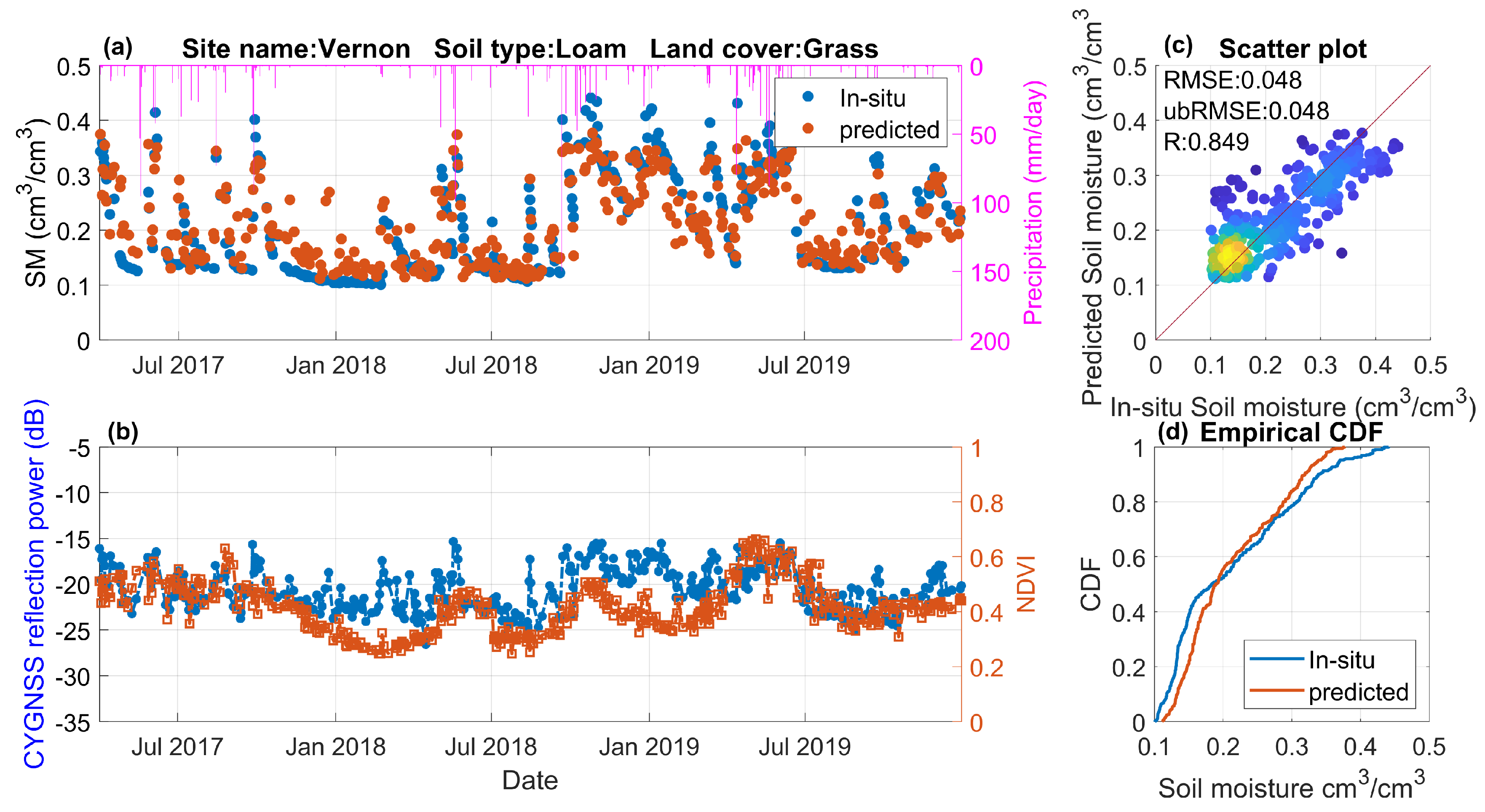
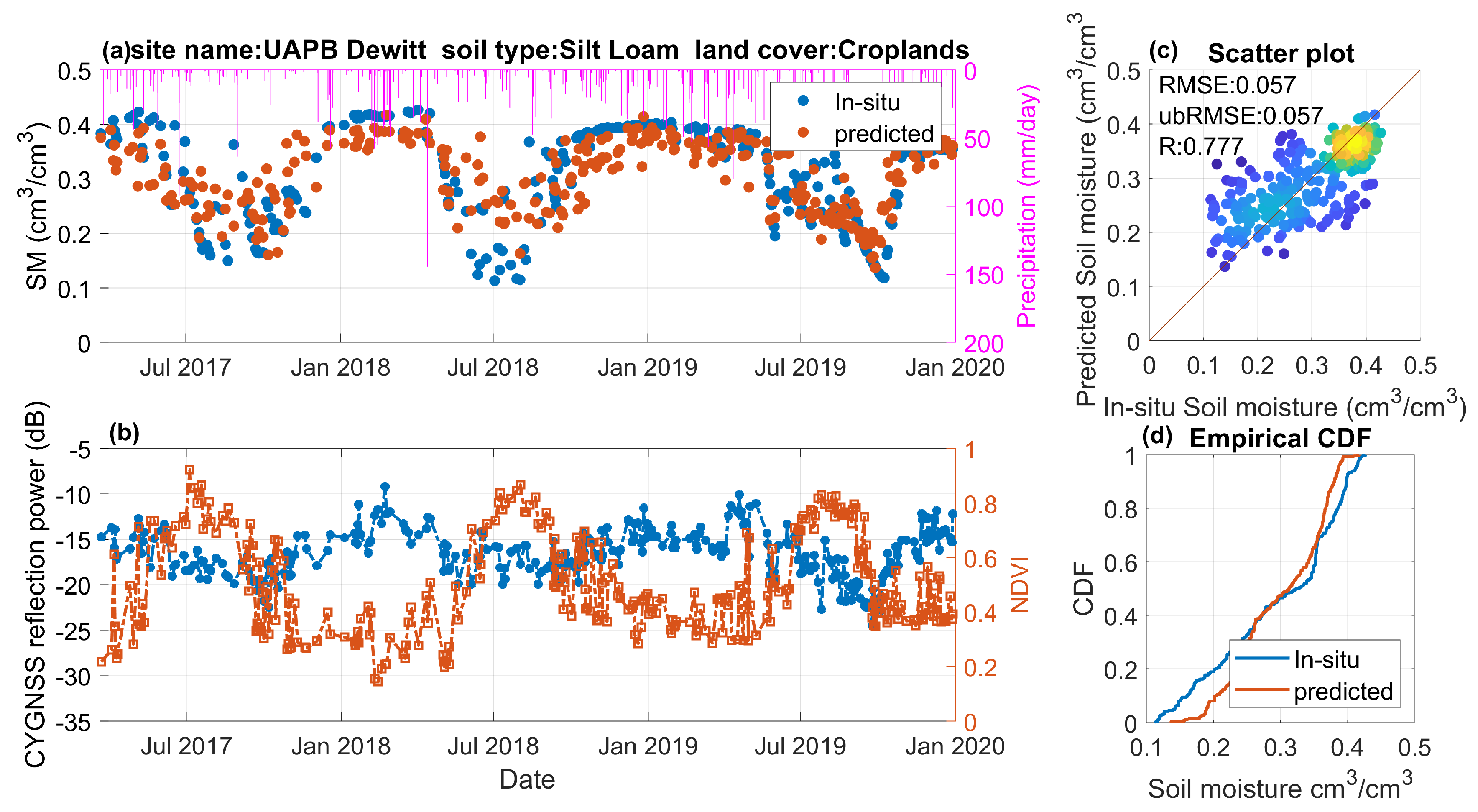
In addition to evaluating the overall performance metrics, it is important to understand the ML-based model’s capability for capturing SM temporal variations. Here, two representative sites are selected and demonstrated in Figure 12 and Figure 13. For both sites, the predicted SM estimates closely follow the temporal trend of the SM observations and correctly capture the precipitation events and the drydown process (Figure 12a and Figure 13a). It is interesting that the CYGNSS reflectivity estimates have a generally good correlation with SM and NDVI for the site with grass land cover type (Figure 12b). For the cropland site shown in Figure 13, NDVI is high (NDVI > 0.7 [-]) and the soil is relatively dry (SM < 0.3 cm/cm) for the growing season (from May to September). The CYGNSS reflectivity well captures the soil water condition instead of the vegetation information. Generally, the predicted and observed SM estimates are align with the 1:1 line (Figure 12c and Figure 13c), and the empirical cumulative distribution function (CDF) lines (Figure 12d and Figure 13d) further validate the high accuracy of predicted SM estimates.
As demonstrated previously in Section 4.2, there are several sites with low R values. When examining the land surface conditions of these sites, it is clearly seen that these sites are highly heterogeneous with mixed grass, crops, savanna, surface water and occasionally urban land cover types. The high heterogeneity not only can decrease the representativeness of in-situ SM observations, but also it can lower the signal-to-noise ratio of CYGNSS observables leading to more problematic input features and reference labels for the ML process. Nevertheless, the relatively low accuracy of these few sites does not contradict the overall high performance of RF-based retrieval model.
5. Discussion
There is a growing interest within the hydrology community to utilize spaceborne GNSS-R observations in SM retrievals. This trend has been particularly accelerated with the availability of recent spaceborne GNSS-R observatories such as TDS-1 and CYGNSS. The allure for using such techniques resides in GNSS-R’s relatively high spatial footprint over smooth Earth surface with frequent observation capabilities. This potential can open new applications in hydrometeorology, atmospheric research, and water resource management at microscale and mesoscale resolutions. The goal of this paper’s research is to exploit CYGNSS data at high spatio-temporal resolution by taking advantage of recent developments in machine learning algorithms that are excellent function approximators and have a remarkable capability in learning complex and nonlinear relationships. The choice of ML approach particularly stems from the challenges of CYGNSS’s pseudorandomly sampled measurements and sensitivity to fine-scale surface features which are challenging to manage at high spatiotemporal resolutions within a physics-based modeling framework. However, effective utilization of an ML algorithm for SM retrievals requires well prepared data which are labeled and include reliable, physics-based ancillary input features in training phase.
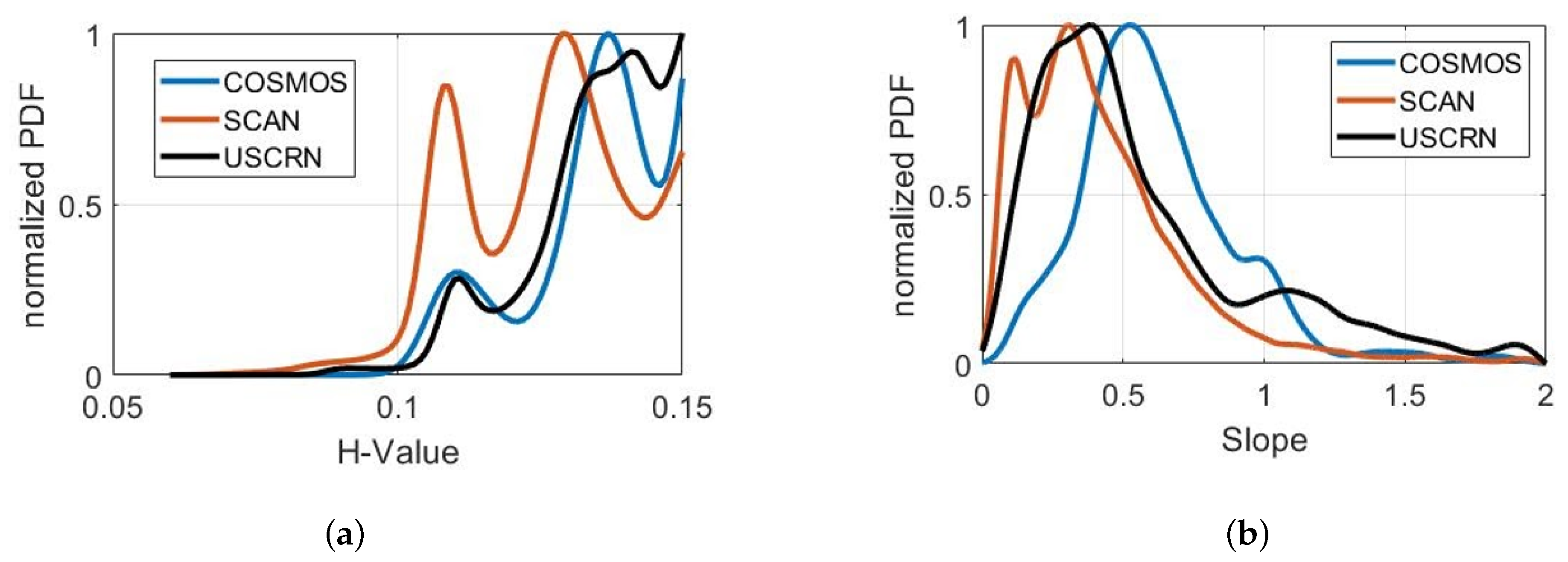
The large number of ISMN sites over CONUS provides an opportunity to extensively exploit ML approaches. Our analysis with ISMN sites demonstrates the potentiality of the ML-algorithms in SM retrievals over various underlying land surface conditions such as soil textures and land covers at high spatio-temporal resolutions. Particularly, the performance over croplands and sandy loam soil provide promising results with higher accuracy. The achieved accuracy is further improved when the ML-model is trained and tested over individual SM networks as opposed to combining all available SM networks. In addition, the generalized methodology is investigated in both space and time using site-independent and year-based cross-validation. The ML-based model is able to capture the temporal variation with variable biases, and the results indicate the importance of a priori information on the prediction capability of the ML-based model. While soil texture features are identified as the most influential ancillary input for the SM prediction, both H-parameter and slope are determined as two least significant features in our ML-model. This result is somewhat surprising from a physics-based perspective since the small-scale roughness and topography are two important factors that can alter the relative contributions of the coherent/incoherent energy observed in CYGNSS measurements. This result could be attributed to the locations of ISMN sites which do not show significant variations within and across individual SM network types in either slope or H-value as shown in Figure 14. This indicates that the sites are located on relatively flat surfaces and that coherent reflections are dominant. However, even if those grid cells are perfectly flat (although somewhat tilted), naturally, a small-scale surface roughness of the order of the wavelength is always present. Spatial and temporal changes of the decoherence due to surface roughness would interfere with the analogous changes in the SM. Future studies perhaps could leverage physics-based modeling frameworks by guiding the ML models with simulations to quantify potential source of errors in the retrievals in the absence of alternative ancillary data.
The correlation coefficient between the in-situ data and spaceborne SM retrieval depends on the number of measurements and the dynamic range of the data. The overall performance of the proposed algorithm should be evaluated over data from all sites which provide a wider dynamic range and higher number of observations. As it is also shown in Table 3, correlation coefficient is over 0.8 in all cases where the method is tested for more than a single site. In terms of averaging for each site, both the number of measurements and the dynamic range of each site are lower leading to comparably lower correlation values. Also for small number of measurements, the effects of outliers and the uncertainty of correlation can be higher. It is definitely a goal to obtain higher correlation for each site in future studies. This could be done through site-based learning approaches or developing a model for a group of highly similar sites.
The proposed methodology is potentially limited to similar terrains for which there exist in-situ data. Direct application of this paper’s ML-model to Earth surfaces beyond CONUS requires further study since the land conditions at ISMN sites are not expected to be representative of the majority of the land scenes crossed by the CYGNSS flight tracks. However, the earth surfaces could be grouped into similar land types by soil texture, topography, and land cover. Perhaps several ML-models for each group could be investigated. In addition, reliable metrics are needed for the ML-based models to learn heterogeneous and mixed scenes which do not necessarily lead to strong coherent reflections. Future work will be needed to fully utilize CYGNSS data for a quasi-global SM data product. This can, perhaps, be achieved by using the SMAP-based SM data as the reference [42]. The key difference between the ISMN and SMAP as the reference label will be the spatial scale. The mismatch of spatial scale representativeness and land surface heterogeneity effects will need further investigation.
6. Conclusions
In this work, an ML-based framework has been presented for estimating SM using the CYGNSS observations over ISMN sites in CONUS. Three widely-used ML algorithms have been tested and validated, among which the RF is observed to be the optimal ML inversion method for this study. A feature selection process reduces the algorithm complexity with a refined input feature set. Several key features are identified, including CYGNSS reflectivity, TES, incidence angle, NDVI, VWC, terrain elevation, and the soil’s silt and clay proportions. Using RF as the utilized ML algorithm and with selected input features, an overall ubRMSE of 0.052 cm/cm is achieved via the 5-fold cross validation strategy. More importantly, sufficient accuracy can be obtained via the site-independent (ubRMSE of 0.054 cm/cm) and year-based (ubRMSE less than 0.050 cm/cm) validation methods, suggesting that the proposed ML-based SM retrieval model can be generalized in space and time with promising confidence. Additionally, the ML inversion performance can be further improved when the training process is separately conducted for different SM observation networks. Although the scale of in-situ SM data from different networks varies, the results demonstrated here indicate that a proper consideration of the spatial scales of CYGNSS observations, soil moisture reference data, and ancillary land surface conditions is important for accurately retrieving SM estimates. Meanwhile, the ML-based model performance is analyzed with respect to the land cover and soil texture conditions. Particularly, soil texture features are identified as the most influential ancillary input for the SM prediction. Overall, the ML model predicted SM estimates have high accuracy for croplands (with ubRMSE less than 0.05 cm/cm), indicating that the ML-based SM retrieval framework can be applied for agricultural soil water monitoring.
Author Contributions
Conceptualization: M.K. and A.C.G.; Methodology: M.K. and A.C.G.; Software: V.S. and F.L.; Validation: V.S. and F.L.; Formal analysis: V.S and F.L.; Investigation: V.S., F.L., D.B., M.K., and A.C.G.; Resources: M.K. and A.C.G.; Data curation: F.L.; Writing–original draft preparation: V.S., F.L., M.K., D.B., and A.C.G.; Writing–review and editing: V.S., F.L., M.K., D.B., A.C.G., and R.M.; Visualization: V.S., F.L., and D.B.; Supervision: M.K. and A.C.G.; Project administration: M.K. and A.C.G.; Funding acquisition: M.K., A.C.G., and R.M. All authors have read and agreed to the published version of the manuscript.
Funding
This research was funded by USDA Agricultural Research Service(USDA-ARS), Award NACA 58-6064-9-007.
Conflicts of Interest
The authors declare no conflict of interest.
References
- Vereecken, H.; Huisman, J.; Bogena, H.; Vanderborght, J.; Vrugt, J.; Hopmans, J. On the value of soil moisture measurements in vadose zone hydrology: A review. Water Resour. Res. 2008, 44. [Google Scholar] [CrossRef] [Green Version]
- Kerr, Y.H.; Al-Yaari, A.; Rodriguez-Fernandez, N.; Parrens, M.; Molero, B.; Leroux, D.; Bircher, S.; Mahmoodi, A.; Mialon, A.; Richaume, P.; et al. Overview of SMOS performance in terms of global soil moisture monitoring after six years in operation. Remote Sens. Environ. 2016, 180, 40–63. [Google Scholar] [CrossRef]
- Colliander, A.; Jackson, T.J.; Bindlish, R.; Chan, S.; Das, N.; Kim, S.; Cosh, M.; Dunbar, R.; Dang, L.; Pashaian, L.; et al. Validation of SMAP surface soil moisture products with core validation sites. Remote Sens. Environ. 2017, 191, 215–231. [Google Scholar] [CrossRef]
- Brocca, L.; Ciabatta, L.; Massari, C.; Camici, S.; Tarpanelli, A. Soil Moisture for Hydrological Applications: Open Questions and New Opportunities. Water 2017, 9, 140. [Google Scholar] [CrossRef]
- Santanello, J.A.; Lawston, P.; Kumar, S.; Dennis, E. Understanding the Impacts of Soil Moisture Initial Conditions on NWP in the Context of Land-Atmosphere Coupling. J. Hydrometeorol. 2019, 20, 793–819. [Google Scholar] [CrossRef]
- Zavorotny, V.U.; Gleason, S.; Cardellach, E.; Camps, A. Tutorial on remote sensing using GNSS bistatic radar of opportunity. IEEE Geosci. Remote Sens. Mag. 2014, 2, 8–45. [Google Scholar] [CrossRef] [Green Version]
- Komjathy, A.; Armatys, M.; Masters, D.; Axelrad, P.; Zavorotny, V.; Katzberg, S. Retrieval of ocean surface wind speed and wind direction using reflected GPS signals. J. Atmos. Ocean. Technol. 2004, 21, 515–526. [Google Scholar] [CrossRef] [Green Version]
- Valencia, E.; Zavorotny, V.U.; Akos, D.M.; Camps, A. Using DDM asymmetry metrics for wind direction retrieval from GPS ocean-scattered signals in airborne experiments. IEEE Trans. Geosci. Remote Sens. 2013, 52, 3924–3936. [Google Scholar] [CrossRef]
- Guan, D.; Park, H.; Camps, A.; Wang, Y.; Onrubia, R.; Querol, J.; Pascual, D. Wind direction signatures in GNSS-R observables from space. Remote Sens. 2018, 10, 198. [Google Scholar] [CrossRef] [Green Version]
- Li, W.; Cardellach, E.; Fabra, F.; Ribó, S.; Rius, A. Assessment of Spaceborne GNSS-R Ocean Altimetry Performance Using CYGNSS Mission Raw Data. IEEE Trans. Geosci. Remote Sens. 2019, 58, 238–250. [Google Scholar] [CrossRef]
- Rodriguez-Alvarez, N.; Holt, B.; Jaruwatanadilok, S.; Podest, E.; Cavanaugh, K.C. An Arctic sea ice multi-step classification based on GNSS-R data from the TDS-1 mission. Remote Sens. Environ. 2019, 230, 111202. [Google Scholar] [CrossRef]
- Santi, E.; Paloscia, S.; Pettinato, S.; Fontanelli, G.; Clarizia, M.; Guerriero, L.; Pierdicca, N. Forest Biomass Estimate on Local and Global Scales Through GNSS Reflectometry Techniques. In Proceedings of the IGARSS 2019—2019 IEEE International Geoscience and Remote Sensing Symposium, Yokohama, Japan, 28 July–2 August 2019; pp. 8680–8683. [Google Scholar]
- Rodriguez-Alvarez, N.; Podest, E.; Jensen, K.; McDonald, K.C. Classifying Inundation in a Tropical Wetlands Complex with GNSS-R. Remote Sens. 2019, 11, 1053. [Google Scholar] [CrossRef] [Green Version]
- Al-Khaldi, M.M.; Johnson, J.T.; O’Brien, A.J.; Balenzano, A.; Mattia, F. Time-Series Retrieval of Soil Moisture Using CYGNSS. IEEE Trans. Geosci. Remote Sens. 2019, 57, 4322–4331. [Google Scholar] [CrossRef]
- Chew, C.; Small, E. Soil moisture sensing using spaceborne GNSS reflections: Comparison of CYGNSS reflectivity to SMAP soil moisture. Geophys. Res. Lett. 2018, 45, 4049–4057. [Google Scholar] [CrossRef] [Green Version]
- Clarizia, M.P.; Pierdicca, N.; Costantini, F.; Floury, N. Analysis of CYGNSS Data for Soil Moisture Retrieval. IEEE J. Sel. Top. Appl. Earth Obs. Remote Sens. 2019, 12, 2227–2235. [Google Scholar] [CrossRef]
- Kim, H.; Lakshmi, V. Use of Cyclone Global Navigation Satellite System (CYGNSS) observations for estimation of soil moisture. Geophys. Res. Lett. 2018, 45, 8272–8282. [Google Scholar] [CrossRef] [Green Version]
- Eroglu, O.; Kurum, M.; Boyd, D.; Gurbuz, A.C. High Spatio-Temporal Resolution CYGNSS Soil Moisture Estimates Using Artificial Neural Networks. Remote Sens. 2019, 11, 2272. [Google Scholar] [CrossRef] [Green Version]
- Ruf, C.; Asharaf, S.; Balasubramaniam, R.; Gleason, S.; Lang, T.; McKague, D.; Twigg, D.; Waliser, D. In-orbit performance of the constellation of CYGNSS hurricane satellites. Bull. Am. Meteorol. Soc. 2019, 100, 2009–2023. [Google Scholar] [CrossRef]
- Ruf, C.S.; Gleason, S.; McKague, D.S. Assessment of CYGNSS wind speed retrieval uncertainty. IEEE J. Sel. Top. Appl. Earth Obs. Remote Sens. 2018, 12, 87–97. [Google Scholar] [CrossRef]
- Wang, T.; Ruf, C.S.; Block, B.; McKague, D.S.; Gleason, S. Design and performance of a GPS constellation power monitor system for improved CYGNSS L1B calibration. IEEE J. Sel. Top. Appl. Earth Obs. Remote Sens. 2018, 12, 26–36. [Google Scholar] [CrossRef]
- McKague, D.S.; Ruf, C.S. On-orbit trending of CYGNSS data. In Proceedings of the IGARSS 2019—2019 IEEE International Geoscience and Remote Sensing Symposium, Yokohama, Japan, 28 July–2 August 2019; pp. 8722–8724. [Google Scholar]
- Gleason, S.; Ruf, C.S.; O’Brien, A.J.; McKague, D.S. The CYGNSS Level 1 calibration algorithm and error analysis based on on-orbit measurements. IEEE J. Sel. Top. Appl. Earth Obs. Remote Sens. 2018, 12, 37–49. [Google Scholar] [CrossRef]
- Carreno-Luengo, H.; Lowe, S.; Zuffada, C.; Esterhuizen, S.; Oveisgharan, S. Spaceborne GNSS-R from the SMAP mission: First assessment of polarimetric scatterometry over land and Cryosphere. Remote Sens. 2017, 9, 362. [Google Scholar] [CrossRef] [Green Version]
- Dorigo, W.A.; Wagner, W.; Hohensinn, R.; Hahn, S.; Paulik, C.; Xaver, A.; Gruber, A.; Drusch, M.; Mecklenburg, S.; Oevelen, P.V.; et al. The International Soil Moisture Network: A data hosting facility for global in situ soil moisture measurements. Hydrol. Earth Syst. Sci. 2011, 15, 1675–1698. [Google Scholar] [CrossRef] [Green Version]
- Dorigo, W.A.; Xaver, A.; Vreugdenhil, M.; Gruber, A.; Hegyiova, A.; Sanchis-Dufau, A.D.; Zamojski, D.; Cordes, C.; Wagner, W.; Drusch, M. Global automated quality control of in situ soil moisture data from the International Soil Moisture Network. Vadose Zone J. 2013, 12. [Google Scholar] [CrossRef]
- Gruber, A.; Dorigo, W.A.; Zwieback, S.; Xaver, A.; Wagner, W. Characterizing coarse-scale representativeness of in situ soil moisture measurements from the International Soil Moisture Network. Vadose Zone J. 2013, 12. [Google Scholar] [CrossRef] [Green Version]
- O’Neill, P.E.; Njoku, E.G.; Jackson, T.J.; Chan, S.; Bindlish, R. SMAP Algorithm Theoretical Basis Document: Level 2 & 3 Soil Moisture (Passive) Data Products; Jet Propulsion Laboratory, California Institute of Technology: Pasadena, CA, USA, 2015; p. JPL D-66480.
- Carreno-Luengo, H.; Luzi, G.; Crosetto, M. Impact of the elevation angle on CYGNSS GNSS-R bistatic reflectivity as a function of effective surface roughness over land surfaces. Remote Sens. 2018, 10, 1749. [Google Scholar] [CrossRef] [Green Version]
- Pekel, J.F.; Cottam, A.; Gorelick, N.; Belward, A.S. High-resolution mapping of global surface water and its long-term changes. Nature 2016, 540, 418. [Google Scholar] [CrossRef]
- Hengl, T.; de Jesus, J.; Heuvelink, G.B.; Gonzalez, M.R.; Kilibarda, M.; Blagotić, A.; Shangguan, W.; Wright, M.N.; Geng, X.; Bauer-Marschallinger, B.; et al. SoilGrids250m: Global gridded soil information based on machine learning. PLoS ONE 2017, 12, e0169748. [Google Scholar] [CrossRef] [Green Version]
- Balakhder, A.M.; Al-Khaldi, M.M.; Johnson, J.T. On the coherency of ocean and land surface specular scattering for GNSS-R and signals of opportunity systems. IEEE Trans. Geosci. Remote Sens. 2019, 57, 10426–10436. [Google Scholar] [CrossRef]
- O’Neill, P.; Chan, S.; Njoku, E.; Jackson, T.; Bindlish, R. SMAP Enhanced L3 Radiometer Global Daily 9 km EASE-Grid Soil Moisture; Version 1. [SPL3SMP _ E]; NASA National Snow and Ice Data Center Distributed Active Archive Center: Boulder, CO, USA, 2016. [Google Scholar]
- Konings, A.G.; Entekhabi, D.; Chan, S.K.; Njoku, E.G. Effect of Radiative Transfer Uncertainty on L-Band Radiometric Soil Moisture Retrieval. IEEE Trans. Geosci. Remote Sens. 2011, 49, 2686–2698. [Google Scholar] [CrossRef]
- Wasserman, P.D. Neural Computing: Theory and Practice; Van Nostrand Reinhold Co.: New York, NY, USA, 1989. [Google Scholar]
- Cortes, C.; Vapnik, V. Support Vector Networks. Mach. Learn. 1995, 20, 273–295. [Google Scholar] [CrossRef]
- Drucker, H.; Burges, C.J.; Kaufman, L.; Smola, A.J.; Vapnik, V. Support vector regression machines. In Advances in Neural Information Processing Systems; MIT Press: Cambridge, MA, USA, 1997; pp. 155–161. [Google Scholar]
- Cutler, A.; Cutler, D.R.; Stevens, J.R. Random forests. In Ensemble Machine Learning; Springer: Berlin, Germany, 2012; pp. 157–175. [Google Scholar]
- Senyurek, V.; Imtiaz, M.; Belsare, P.; Tiffany, S.; Sazonov, E. Cigarette Smoking Detection with An Inertial Sensor and A Smart Lighter. Sensors 2019, 19, 570. [Google Scholar] [CrossRef] [PubMed] [Green Version]
- Marcano-Cedeno, A.; Quintanilla-Domínguez, J.; Cortina-Januchs, M.; Andina, D. Feature selection using sequential forward selection and classification applying artificial metaplasticity neural network. In Proceedings of the IECON 2010—36th Annual Conference on IEEE Industrial Electronics Society, Glendale, AZ, USA, 7–10 November 2010; pp. 2845–2850. [Google Scholar]
- Zreda, M.; Desilets, D.; Ferré, T.; Scott, R. Measuring soil moisture content non-invasively at intermediate spatial scale using cosmic-ray neutrons. Geophys. Res. Lett. 2008, 35, L21402. [Google Scholar] [CrossRef] [Green Version]
- Fangni, L.; Senyurek, V.; Boyd, D.; Kurum, M.; Gurbuz, A.; Moorhead, R. Machine-Learning based retrieval of Soil Moisture at High Spatio-temporal Scales Using CYGNSS and SMAP Observations. In Proceedings of the IGARSS 2020 IEEE International Geoscience and Remote Sensing Symposium, Waikoloa, HI, USA, 19–24 July 2020. [Google Scholar]
Figure 1.
The spatial distribution map of the International Soil Moisture Network (ISMN) sites. Sites shown in gray are excluded based on the masking criteria described in Section 2.4.
Figure 1.
The spatial distribution map of the International Soil Moisture Network (ISMN) sites. Sites shown in gray are excluded based on the masking criteria described in Section 2.4.

Figure 2.
Flowchart of the proposed soil moisture (SM) retrieval algorithm.

Figure 3.
Root-mean-square-error (RMSE) of the training and testing data as a function of the model complexity for three different ML algorithms: (a) Artificial Neural Network (ANN), (b) Random Forest (RF), and (c) Support Vector Machine (SVM).
Figure 3.
Root-mean-square-error (RMSE) of the training and testing data as a function of the model complexity for three different ML algorithms: (a) Artificial Neural Network (ANN), (b) Random Forest (RF), and (c) Support Vector Machine (SVM).

Figure 4.
Scatter plots of the predicted SM estimates versus in-situ SM observations for ML models with different input feature groups. The input features are described in Table 2. Color of scatter points indicates the density of data points where yellow means a dense data sampling.
Figure 4.
Scatter plots of the predicted SM estimates versus in-situ SM observations for ML models with different input feature groups. The input features are described in Table 2. Color of scatter points indicates the density of data points where yellow means a dense data sampling.

Figure 5.
The RMSE values of the sequential feature selection through (a) forward and (b) backward selection sequences.
Figure 5.
The RMSE values of the sequential feature selection through (a) forward and (b) backward selection sequences.

Figure 6.
(a) The scatter plot of the predicted SM versus in-situ SM through a RF-based model with 8 selected input features and (b) the Taylor diagram for all sites.
Figure 6.
(a) The scatter plot of the predicted SM versus in-situ SM through a RF-based model with 8 selected input features and (b) the Taylor diagram for all sites.

Figure 7.
Spatial distribution maps of the (a) unbiased RMSE (ubRMSE) and (b) correlation coefficient (R) for all sites over contiguous U.S. The sizes of the filled circles are scaled as a function of the number of observations.
Figure 7.
Spatial distribution maps of the (a) unbiased RMSE (ubRMSE) and (b) correlation coefficient (R) for all sites over contiguous U.S. The sizes of the filled circles are scaled as a function of the number of observations.

Figure 8.
Scatter plots of SM retrievals for different types of soil texture.

Figure 9.
Scatter plots of SM retrievals for different types of vegetation land cover.

Figure 10.
SM prediction performance (ubRMSE value) comparison for varying soil texture and land cover types.
Figure 10.
SM prediction performance (ubRMSE value) comparison for varying soil texture and land cover types.

Figure 11.
Scatter plots and performance metrics of multiple ML models for each network type: (a) the COsmic-ray Soil Moisture Observing System (COSMOS), (b) the Soil Climate Analysis Network (SCAN), and (c) U.S. Climate Reference Network (USCRN).
Figure 11.
Scatter plots and performance metrics of multiple ML models for each network type: (a) the COsmic-ray Soil Moisture Observing System (COSMOS), (b) the Soil Climate Analysis Network (SCAN), and (c) U.S. Climate Reference Network (USCRN).

Figure 12.
Comparison of (a) the in-situ observed and predicted SM time series and (b) CYGNSS reflectivity and normalized difference vegetation index (NDVI) time series for site Vermon. (c) The scatter plot and (d) cumulative density function (CDF) between predictions and measurements.
Figure 12.
Comparison of (a) the in-situ observed and predicted SM time series and (b) CYGNSS reflectivity and normalized difference vegetation index (NDVI) time series for site Vermon. (c) The scatter plot and (d) cumulative density function (CDF) between predictions and measurements.

Figure 13.
Same as Figure 12 but for site Uapb Dewitt.
Figure 13.
Same as Figure 12 but for site Uapb Dewitt.

Figure 14.
Distribution of (a) small scale roughness (H-value) and (b) topographic slope input features for each SM network.
Figure 14.
Distribution of (a) small scale roughness (H-value) and (b) topographic slope input features for each SM network.


Table 1.
The ISMN data statistics before and after quality control flags.
| Initial | Quality Control Mechanisms and the Ratio on the Raw Dataset | % | Final | |||
|---|---|---|---|---|---|---|
| # of Sites | # of Data | # of Sites | # of Data | |||
| COSMOS | 14 | 7381 | CYGNSS quality flags | 27 | 5 | 1923 |
| SCAN | 104 | Incidence angle > 65∘ | 3 | 68 | ||
| USCRN | 53 | Rx_gain < 0 | 27 | 33 | 8679 | |
| 2017 | 225 | Peak power delay row bin | 20 | 89 | 7580 | |
| 2018 | 219 | Water land percent > 2% | 16.6 | 99 | 9485 | |
| 2019 | 222 | Elevation > 600 m (for 2017) | 11 | 100 | ||
| Overall | 234 | Urban areas | 0.9 | 106 | ||
| VWC > 5 kg/m2 | ||||||
Table 2.
Physical features considered for the machine learning (ML)-based SM retrieval model.
| Input Group | Feature Name | Description |
|---|---|---|
| CYGNSS | Reflectivity | Reflectivity calculated via [13] |
| TES | Slope of the trailing edge of the reflectivity | |
| LES | Leading edge slope of the reflectivity | |
| SP incidence angle | Incidence angle of specular point | |
| Topography | Elevation | Mean elevation for each specular point 3-km grid |
| Slope | Mean Slope for each specular point 3-km grid | |
| MODIS | NDVI | Mean normalized difference vegetation index |
| VWC | Mean vegetation water content | |
| H-value | Dominant land cover type based roughness parameter | |
| Soil texture | Soil clay ratio | Mean clay proportion for each specular point 3-km grid |
| Soil silt ratio | Mean silt proportion for each specular point 3-km grid | |
| Soil sand ratio | Mean sand proportion for each specular point 3-km grid |
Table 3.
Overall and site-averaged performance metrics for different cross-validation methods. Numbers in parentheses are the standard deviation (std.) of metrics across different sites.
Table 3.
Overall and site-averaged performance metrics for different cross-validation methods. Numbers in parentheses are the standard deviation (std.) of metrics across different sites.
| Validation Method | Overall Performance | Average of Sites | |||||
|---|---|---|---|---|---|---|---|
| RMSE | ubRMSE | R | RMSE (std.) | bias (std.) | ubRMSE (std.) | R value (std.) | |
| 5fold | 0.0523 | 0.0523 | 0.89 | 0.050 () | 0.011 () | 0.047 () | 0.56 () |
| Site independent | 0.0883 | 0.0883 | 0.64 | 0.084 () | 0.056 () | 0.054 () | 0.42 () |
| year based (2019) | 0.0639 | 0.0639 | 0.84 | 0.06 () | 0.027 () | 0.05 () | 0.49 () |
| year based (2018) | 0.0586 | 0.0584 | 0.86 | 0.055 () | 0.024 () | 0.047 () | 0.43 () |
| year based (2017) | 0.0602 | 0.0599 | 0.84 | 0.058 () | 0.027 () | 0.048 () | 0.40 () |
Table 4.
Overall and averaged performance metrics for multiple ML models based on SM networks. Numbers in parentheses are the standard deviations of metrics across different network-based models.
Table 4.
Overall and averaged performance metrics for multiple ML models based on SM networks. Numbers in parentheses are the standard deviations of metrics across different network-based models.
| RMSE | Bias | ubRMSE | R | |
|---|---|---|---|---|
| Overall | 0.049 | −1 × 10⁻⁴ | 0.049 | 0.9 |
| Average of sites | 0.048() | 0.0085() | 0.046() | 0.58() |
© 2020 by the authors. Licensee MDPI, Basel, Switzerland. This article is an open access article distributed under the terms and conditions of the Creative Commons Attribution (CC BY) license (http://creativecommons.org/licenses/by/4.0/).
Share and Cite
MDPI and ACS Style
Senyurek, V.; Lei, F.; Boyd, D.; Kurum, M.; Gurbuz, A.C.; Moorhead, R. Machine Learning-Based CYGNSS Soil Moisture Estimates over ISMN sites in CONUS. Remote Sens. 2020, 12, 1168. https://0-doi-org.brum.beds.ac.uk/10.3390/rs12071168
AMA Style
Senyurek V, Lei F, Boyd D, Kurum M, Gurbuz AC, Moorhead R. Machine Learning-Based CYGNSS Soil Moisture Estimates over ISMN sites in CONUS. Remote Sensing. 2020; 12(7):1168. https://0-doi-org.brum.beds.ac.uk/10.3390/rs12071168
Chicago/Turabian StyleSenyurek, Volkan, Fangni Lei, Dylan Boyd, Mehmet Kurum, Ali Cafer Gurbuz, and Robert Moorhead. 2020. "Machine Learning-Based CYGNSS Soil Moisture Estimates over ISMN sites in CONUS" Remote Sensing 12, no. 7: 1168. https://0-doi-org.brum.beds.ac.uk/10.3390/rs12071168
Note that from the first issue of 2016, this journal uses article numbers instead of page numbers. See further details here.