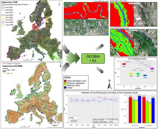
Object-Based Ensemble Learning for Pan-European Riverscape Units Mapping Based on Copernicus VHR and EU-DEM Data Fusion

Abstract

Recent developments in the fields of geographical object-based image analysis (GEOBIA) and ensemble learning (EL) have led the way to the development of automated processing frameworks suitable to tackle large-scale problems. Mapping riverscape units has been recognized in fluvial remote sensing as an important concern for understanding the macrodynamics of a river system and, if applied at large scales, it can be a powerful tool for monitoring purposes. In this study, the potentiality of GEOBIA and EL algorithms were tested for the mapping of key riverscape units along the main European river network. The Copernicus VHR Image Mosaic and the EU Digital Elevation Model (EU-DEM)—both made available through the Copernicus Land Monitoring Service—were integrated within a hierarchical object-based architecture. In a first step, the most well-known EL techniques (bagging, boosting and voting) were tested for the automatic classification of water, sediment bars, riparian vegetation and other floodplain units. Random forest was found to be the best-to-use classifier, and therefore was used in a second phase to classify the entire object-based river network. Finally, an independent validation was performed taking into consideration the polygon area within the accuracy assessment, hence improving the efficiency of the classification accuracy of the GEOBIA-derived map, both globally and by geographical zone. As a result, we automatically processed almost 2 million square kilometers at a spatial resolution of 2.5 meters, producing a riverscape-units map with a global overall accuracy of 0.915, and with per-class F1 accuracies in the range 0.79–0.97. The obtained results may allow for future studies aimed at quantitative, objective and continuous monitoring of river evolutions and fluvial geomorphological processes at the scale of Europe.

1. Introduction

Hydromorphological pressures affect 40% of European water bodies, hampering the achievement of their good ecological status [1]. Characterizing river morphology is essential in order to identify alterations and design restoration measures. Traditionally, most river geomorphological survey methodologies rely heavily on field-based methods that require time- and resource-intensive field campaigns, resulting in scattered information and sensitive to operator subjectivity [2,3,4]. Fluvial remote sensing, an emerging discipline joining the river science and remote sensing (RS) [5], now offers new possibilities for monitoring river processes at high spatial and temporal resolution, thanks to the exploitation of objective, repeatable and continuous information alongside the entire river network [6]. Unprecedented possibilities are available nowadays for river science and management, from the local, to the regional and, eventually, continental scales.

An essential aspect in river science—both for fluvial processes assessment and for river management purposes—is the delineation of the main riverscape units that characterize the fluvial landscape in the vicinity and within the so-called active river channel [7]. The active channel is defined in literature as the low-flow channel, plus adjacent sediment bars at the edges of perennial, terrestrial vegetation, usually subjected to erosion and deposition processes and by vegetation encroachment [8,9,10]. Mapping riverscape units is important for the understanding of the macrodynamics of a river system and if repeated through time it can be a powerful tool for different purposes, such as the assessment of evolutionary trajectories of river reaches [11], stream fragmentation [12] or human pressures [13,14], just to mention a few.

In the literature, few researchers have attempted to map these key units at the continental scale in an automated/semi-automated way through the use of RS data. Spada et al. [11] analyzed the main Albanian rivers over a 40-year period, extracting the river centerlines, as well as active and wet channel width using multisource satellite data, such as Landsat and Sentinel-2. Bertrand et al. [15] mapped some riverscape units and channel types based on RGB orthophotos for the Drôme catchment (France), using a geographical object based image analysis (GEOBIA) technique. Belletti et al. [16] manually digitized channel boundaries and associated riverscape units on available orthophotos, with the aim of analyzing historical changes in channel morphology for a selection of reaches. In the work of Demarchi et al. [17] the potentiality of GEOBIA and Machine Learning (ML) classification were integrated for the automatic delineation of main riverscape units at the sub-meter resolution (40 cm) for 1200 km of river length of the main river systems of Piedmont Region (Italy). The RS classification map was then used in support of a quantitative river type classification and characterization of fluvial forms across the region. The utility of such type of objective and continuous mapping was also demonstrated by the subsequent work of Bizzi et al. [18], in which a consistent assessment at the regional scale of human-induced 50–100-year channel changes was provided for the first time, thanks to the exploitation of the RS-based riverscape units map.

Over the last two decades, GEOBIA has emerged as a new paradigm in RS analysis, thanks to its capability of boosting classification performances as compared to per-pixel analysis, especially when processing very high-resolution (VHR) multi-spectral data [19,20,21,22,23,24,25]. Research interests have shifted from the development of theoretical foundations toward their implementation in a wide variety of real-world applications [26]. The integration of supervised ML techniques into GEOBIA has helped in reaching such achievements [27]. Ensemble learning (EL) methods have been reported to be the most influential development within ML in the past decade [28,29]. They are able to combine multiple classification models into one final improved result, thanks to different training techniques, namely bagging, boosting or voting. Several studies can be found in literature nowadays where different EL algorithms, mainly random forest, are used for the classification of image objects in a broad range of applications [30,31,32,33]. However, most of these studies, as reviewed in [27], are focused on study areas of less than 300 ha (3 km²), with a spatial resolution of images between 0 and 2 m.

The main objective of this paper is hence to test the capability of GEOBIA combined with EL algorithms in automatizing the segmentation and classification procedures at the big-data scale, for the purpose of mapping the main riverscape units of the main European river network. A hierarchical object-based architecture, developed in a previous study by Demarchi et al. [34] and based on airborne sub-meter orthophotos and LiDAR data, is adapted in the present work for the fusion of two continental-scale datasets: the Copernicus VHR Image Mosaic and the EU Digital Elevation Model (EU-DEM)—both made available through the Copernicus Land Monitoring Service (https://land.copernicus.eu/). Such types of open source VHR satellite data are becoming nowadays more and more available, therefore an adaptation of the previous methodology to a similar spectral and topographic dataset configuration is strongly envisaged. All river segments of Europe with basin area > 5000 km² were selected and the two-level segmentation procedure was implemented for the overlapping 700 image tiles of 50 km*50 km spread around Europe, with the aim of integrating the topographic data with the VHR data in an automated way. After collecting numerous training and validation reference objects by visual inspection, different EL classifiers were trained and tested for the mapping of the main riverscape units: water, sediment bars, riparian vegetation and other floodplain units. Random forest (RF), extra trees (ET), gradient tree boosting (GTB) and extreme gradient boosting (XGB) were tested and finally the different predictions were combined within a voting classifier (VC), one of the simplest ways to combine different ML techniques [35]. In this way, we could attempt to generalize a best-to-use classifier for the object-based classification of riverscape units. The best classifier was then used to predict the label class of all objects produced by GEOBIA at the European scale. Finally, the riverscape units map was validated with an independent set of samples, which resulted in a validated product covering almost 2 million square kilometers at the resolution of 2.5 m. The obtained results allow to shed lights on the usefulness of the Copernicus VHR and EU-DEM products for mapping the main landcovers describing fluvial landscapes at the European scale.

2. Study Area and Data Description

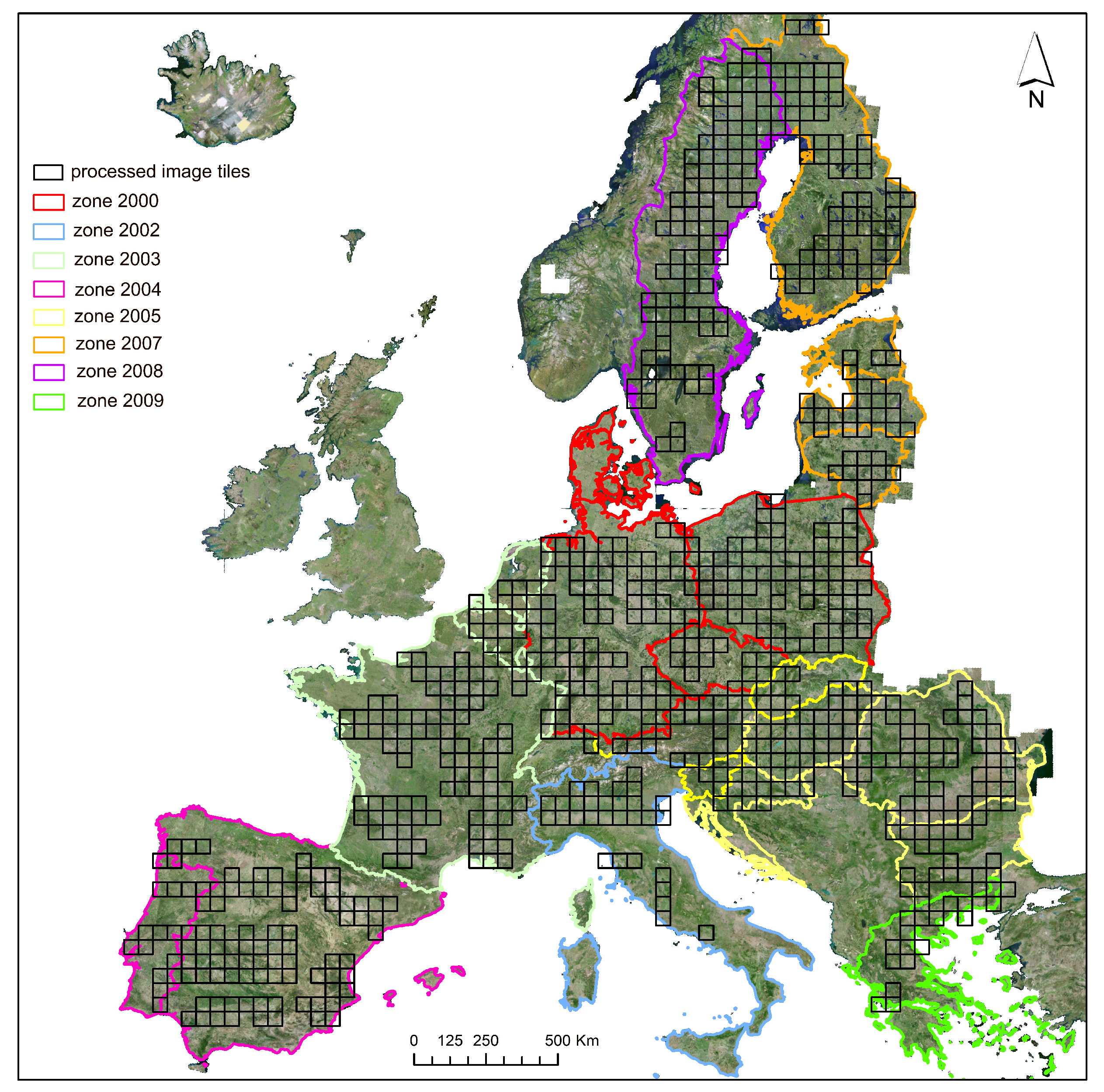
2.1. Remote Sensing Data and Areas of Interest

The focus of this work was on the main river systems of Europe with a basin size larger than a set threshold of 5000 km². This threshold was set to exclude those river systems that would not properly be distinguishable at the scale of EU-DEM and VHR datasets, respectively 25 and 2.5 m. River segments were selected from the catchment characterization model (CCM2) database and divided in geographical zones, according to [36]. Figure 1 shows the Copernicus VHR Image Mosaic, with the selected zones of analysis and the relative image tiles selected for the processing (see also Section 3.1). Selected river segments analyzed in this work overlaid on the EU-DEM layer are instead showed in Figure 2.

The Copernicus VHR Image Mosaic (Figure 1) is a seamless mosaic of very high resolution (VHR), based mainly on SPOT-5/6 and Formosat-2 data. It is available through the Copernicus Land Monitoring Service (https://land.copernicus.eu/) and it was developed to cover various land applications and emergency response services at EU level (e.g., Urban Atlas, Natura 2000 sites, etc.). It covers a surface of 7.3 million square kilometers at a spatial resolution of 2.5 meters and it comprises three spectral bands: red, (0.665 μm), green (0.560 μm) and blue (0.490 μm). The SPOT-5 images have a panchromatic geometry, resulting from the merging of two separate images, one in panchromatic mode at 2.5 m, and the other one in three-band multi-spectral mode at 10-meter spatial resolution. A histogram equalization was applied for best visual impression [37] and a cloud-free optimization resulted in a cloud coverage below 5% per NUTS unit (Nomenclature of territorial units for statistics, [38]).

The Digital Elevation Model over Europe (EU-DEM) (Figure 2) is a digital surface model (DSM) of the EEA39 countries, representing the first surface as illuminated by the sensors, a hybrid product based on SRTM and ASTER GDEM data, fused by a weighted, averaging approach. It was downloaded from the Copernicus Land Monitoring Service website as a mosaic product at 25-m spatial resolution. The final study area extent of this work is the result from the overlap between the Copernicus VHR imagery, EU-DEM and river network with basin area > 5000 km².

The aim of this work is to map the main hydromorphological-significant landcover types that characterize fluvial landscapes in Europe, within the selected area of interest discussed above. Considering the spatial resolutions of both dataset—25 m for the EU-DEM and 2.5 m for the VHR—we decided to target our classification problem to the following classes: water, sediment bars, riparian vegetation and other floodplain units (OFU). The major challenge of mapping these riverscape units automatically using RS data lies in distinguishing sediment bars and riparian vegetation units from those landscape units that can be found within the floodplain (e.g., OFU class) and that have similar spectral characteristics. For example, sediment bars are spectrally comparable with crop fields left fallow due to crop rotation practices or to gravel rural roads or urban settlements that can be found in the floodplain. In fact, discerning between spectrally similar land cover classes such as urban areas and bare soil fields is a huge challenge, even for RS data operating at high spatial and spectral resolution (e.g., hyperspectral data) [39,40]. One of the objectives of this study, is to test the capability of the Copernicus VHR dataset in this context, which comes with a very limited spectral configuration, in particular without the near-infrared spectral band.

In addition, European rivers are characterized by highly diverse and dynamic landforms. Figure 3 pictures some examples of the investigated river sections for this paper. Most representative river types are present in the European landscape, such as meandering, sinuous, wandering and braided, making the GEOBIA segmentation and EL classification an even more challenging problem.

3. Methodology

3.1. Data Pre-Processing and Organization

The different sources of data used in this work and their related processes are summarized in Figure 4. The Copernicus VHR dataset was delivered in the form of tiles of 50 km*50 km. All tiles covering the investigated rivers were selected and organized in a structured database, grouped according to the CCM2 zone subdivision described in Figure 1. In

Table 1. Number of processed tiles and corresponding areas per zone of analysis.

Zones	Description	Number of Tiles	Area (km2)
2000	Germany/Poland	124	310,000
2002	Italy	30	75,000
2003	France/Benelux	126	315,000
2004	Iberian Peninsula	89	222,500
2005	Balkans	145	362,500
2007	Baltics	83	207,500
2008	Sweden	88	220,000
2009	Greece	26	65,000
	Tot	711	1,777,500

the number of tiles and the corresponding processed areas in square kilometers are showed for each zone of analysis.

This structure was used to create different project files under the eCognition Developer 9^® software, which was employed for the first part of the processing: slope calculation and the two-level hierarchical object-based segmentation (explained in Section 3.2). The mosaicked EU-DEM (Figure 2) was clipped according to the Copernicus VHR tile extents and cataloged in the same structured database, using a homogeneous naming convention, so to facilitate the automatic reading procedure when building the different eCognition’s projects. The selected river segments, together with the EU-DEM, were used as input into the “fluvial corridor” toolbox described in Roux et al. [41], useful for the generation of the Valley Bottom (VB) and the detrended digital terrain model (DDTM). The VB, described by Alber and Piégay 2011 [42] as the modern alluvial floodplain, is an important fluvial unit in the geomorphological characterization of stream networks, representing the deposition zone of alluvium, including both riverbed and floodplain areas [43]. All further processing in this study will focus exclusively within the boundaries delineated by the VB shapefile, ignoring everything falling outside. The DDTM represents the elevation of all floodplain pixels with respect to the river channel and it has been proven in both [34] and [17] to be a powerful tool for properly identifying those riverscape units that could present similar spectral characteristics, but different topographical features. The “fluvial corridor” was run for each zone separately. The resulting DDTM rasters (Figure 4) were then clipped and renamed into the same tile grid scheme as used for the EU-EUDEM and VHR database (as explained above). As a result of the pre-processing step, the following layers were automatically loaded in the eCognition’s projects (Figure 4), created for each zone of analysis (Figure 1):

• RED layer, from Copernicus VHR at 2.5 m resolution
• GREEN layer, from Copernicus VHR at 2.5 m resolution
• BLUE layer, from Copernicus VHR at 2.5 m resolution
• DEM layer, from Copernicus EU-DEM at 25 m resolution
• SLOPE layer, computed at 25 m resolution
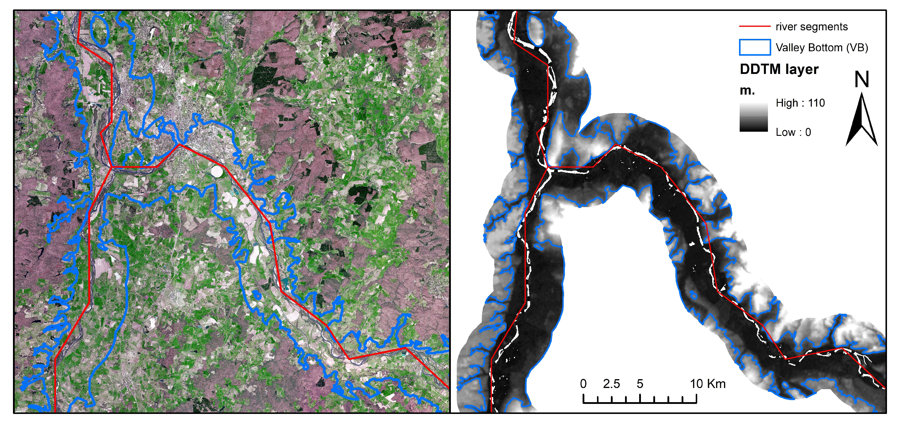
• DDTM layer, computed at 25 m resolution
• VB shapefile

3.2. Two-Level Hierarchical Object-Based Segmentation and Reference Dataset

The geographic, object-based image analysis (GEOBIA) consists in grouping connected pixels with similar spectral characteristics into meaningful image objects, with a similar approach as humans conceptually organize the landscape in order to comprehend it [20]. In this way, a broad range of features can be used to describe individual objects and classification performances can be enhanced [44]. GEOBIA techniques have been applied mainly to VHR imagery, in order to boost their limited spectral range (3–4 bands) [19]. In the previous works of Demarchi et al. 2016 [34] and Demarchi et al. 2017 [17], GEOBIA has proven its potentiality of integrating the spectral bands of VHR imagery with the topographical information coming from simultaneous airborne sub-meter orthophotos and LiDAR data for mapping the riverscape units for the main river network of the Piedmont region (Italy), at the spatial scale of 40 cm.

The riverscape unit segmentation and classification methodology implemented in this study is an adaptation of Demarchi et al. 2017 [17], applied in this case to the main river network of Europe (as explained in Section 2.1), and using only the three RGB spectral bands of the Copernicus VHR dataset. The first step of any GEOBIA procedure is the generation of objects, through the so-called segmentation step. In this study we adopted a two-level hierarchical approach, which has been proven to be an efficient method to well integrate the topographic coarser-resolution information with the higher spatial resolution spectral bands [17,34]. The first level segmentation was generated using a multi-resolution algorithm [44] in eCognition software using the slope layer as a unique input (layer 5 of Figure 4). Hence, specific morphological features of the active river channel, characterized by similar slope values, may be distinguishable. Within these topographically homogenous features a second, finer sub-level segmentation was then produced by using the 3 spectral layers available: Red, Green and Blue (layers 1,2,3 of Figure 4). Performing the hierarchical two-level segmentation proved to facilitate the distinction between the main landcover classes found in the active part of the river channel (for example, sediment bars) from those areas of the floodplain that are characterized by very similar spectral characteristics (for example, arable fields) [34]. For the two-level segmentations the following parameters were used: scale parameter 40, shape coefficient 0.1 and compactness coefficient 0.5. Using the same scale parameter for two sources of data with different spatial resolution, resulted in the generation of smaller objects in the level 2 segmentation, based on spectral differences. The Level 2 segmentation was used for the next step of classification. Therefore, for each object, the mean and standard deviation of the layers 1–6 (Figure 4, RGB bands, EU-DEM, slope and DDTM) were computed and used as input into the classification models. Later, many Level-2 objects were labeled into the investigated classes (water, sediment bars, riparian vegetation and OFU) based on visual inspections, in order to create a vast reference database for a proper training and validation of the classification models. A spatial random sampling technique was adopted as much as possible.

3.3. Ensemble Learning Classification and Validation

Ensemble Learning (EL) classification techniques, based on the combination of multiple classifiers, have proven to be among the most powerful techniques in analyzing RS data, in particular to improve classification results when processing multisource data [45,46,47,48]. EL consists in individually training diverse classifiers and then combine them with various techniques, such as bagging, boosting or voting, to generate the final prediction. The bootstrap aggregation method, also called Bagging, builds an ensemble of learners using the same training algorithm but training each learner with several subsets of data (bags) that are randomly selected with replacement, meaning that the same sample can be selected in different subsets [49]. The output of each model is then combined in a final voting system. The bagging technique is at the base of the well-known random forest (RF) algorithm, which builds multiple decision trees using this technique [50]. The high number of trees and the low correlation between each other’s is the powerfulness of RF, resulting in its massive implementation in several disciplines, among which RS classification and regression [51,52,53,54,55]. Extremely randomized trees or extra trees (ET) are reported to be a new advancement of RF and therefore were also selected for this study [56].

On the other hand, the boosting technique is an ensemble method in which the prediction power is improved by iteratively training a sequence of weak models, each compensating the weaknesses of its predecessors [57,58]. This is realized by adding miss-classified points to the next learner with a higher weight so that the next classifier will pay extra attention to classify them correctly. New weak learners are added sequentially so to focus the training on more difficult patterns. The final predictions are made by majority vote of the weak learners’ predictions, weighted by their individual accuracy. Among these algorithms, the gradient tree boosting (GTB) [59,60,61] and the extreme gradient boosting (XGB) algorithms [62,63,64] have proven to be among the most effective from the ensemble family and are known for outstanding performances and state-of-the-art results in many research areas. In particular, the XGB was reported to be faster, more robust to noise, class imbalance (a problem in our case study) and exhibiting promising performances on classification tasks of RS data, outperforming various benchmark classifiers [65,66,67].

One of the aims of this paper is to shed lights on the proper EL algorithm to be used for object-based classification of riverscape units at the pan-European scale. Therefore, we tested several among the most commonly used EL algorithms: RF and ET, based on the Bagging technique and GTB and XGB based on the boosting technique and then we finally combined the different predictions with a voting classifier (VC), one of the simplest ways to combine different ML techniques [35]. The classification itself was approached in two steps under the Jupyter Notebook using the scikit-learn python library [68]. First, the different EL algorithms were trained and compared with the aim of identifying the most performing one, based on cross-validation metrics. Then, in the second step, the best selected algorithm was run onto the selected river network at pan-European scale. A post-classification, quality control operation was performed in QGIS (Figure 4), in order to visually check and remove major big errors. In the last final step, an independent validation was performed zone by zone and globally for the whole Europe in Jupyter Notebook, with the aim of assessing the real quality of the produced pan-European riverscape units map.

The assessment of GEOBIA products has specific issues as compared to standard pixel-based classification results. In recent years, new GEOBIA accuracy assessment methods are emerging, highlighting the drawbacks of point-based assessment methods, which consider each polygon as an individual sampling unit, without taking into account its area [27]. However, the variable polygon size is a major concern in assessing a GEOBIA-derived map. In fact, classification accuracy depends also on the polygon area. Adding the polygon area within the accuracy assessment could help improving the efficiency of the classification accuracy of a GEOBIA-derived map [69]. Therefore, in this paper we tested both point-based and area-based accuracy assessments, and computed accuracy indices both zone by zone and for the whole zones together (global assessment).

4. Results

4.1. Pre-Processing and GEOBIA Segmentation Results

An example of the “fluvial corridor” toolbox outputs (Section 3.1, Figure 4), used for calculating the VB shapefile and the DDTM raster layer, is presented in Figure 5. The first one depicts the river floodplain, within which all analysis performed in this study were focused on, while the second one represents the elevation of any floodplain pixel with respect to the water channel. In Figure 6, the spatial distribution of the resulting VB shapefiles for all zones analyzed are displayed.

The two-level hierarchical segmentation processing was the most time demanding effort of the whole implementation methodology, requiring a total of about 25 days of processing time. The processing was performed on a local machine, using an Intel^® Xeon^® CPU @ 3.30 GHz with 16 GB of RAM (Intel Polska, Warsaw). The resulting time of the segmentation process divided by zone, is reported in

Table 2. Two-level hierarchical segmentation processing time displayed by zone of analysis.

Zones	Minutes	Hours	Days	Average Per Tile (min)
2000	6039	100.7	4.2	48.7
2002	1480	24.7	1.0	49.3
2003	6720	112.0	4.7	53.3
2004	4470	74.5	3.1	50.2
2005	7380	123.0	5.1	50.9
2007	4365	72.8	3.0	52.6
2008	4830	80.5	3.4	54.9
2009	1380	23.0	1.0	53.1
		tot	25.5	51.6

.

Results of the two-level, object-based segmentation (Figure 7) show that the adopted GEOBIA segmentation is well representing the different landscape features that can be found within different types of river floodplain around Europe. The next step was the collection of different reference samples to be used for building the EL algorithms (Section 3.1, Figure 4) and for the validation of the final classification map. Therefore, several objects were labeled into the investigated classes (water, sediment bars, riparian vegetation and OFU), using a spatial random sampling approach, as showed in Figure 8.

The selected image tiles where reference samples were collected is plotted in Figure 6 in green boxes. As we can see, a quite good geographical distribution of reference samples was realized, well depicting the high heterogeneity of the analyzed landcover classes around Europe. This was an extensive time-demanding operation, which resulted in a high number of reference objects (as showed in

Table 3. Number of reference objects to be used for classification, for each zone and class.

Code	Class	2000	2002	2003	2004	2005	2007	2008	2009
1	OFU	29,059	9999	31,582	9886	34,106	4977	8018	17,343
2	RV	1131	1131	6348	413	14,207	2861	692	14,343
3	SB	908	908	978	159	592	8	75	396
4	W	825	825	2826	2885	2220	2064	1877	652
	tot	31,923	12,863	41,734	13,343	51,125	9910	10,662	32,734

), to be used for training/validation purposes. The variable number of objects indicated in Table 3 is mainly determined by the occurrence of such landcover types in naturally different river landscapes through Europe and by the fact that OFU is representing a much higher variability of landcover types, as compared to other classes. For each sample, the mean and standard deviation of all input layers (RGB bands, DEM, slope and DDTM) were computed in eCognition software and exported, so to be read into the Jupyter Notebook in the next following step: training and validation of the EL algorithms (Section 3.1, Figure 4).

4.2. Ensemble Learning Modelling Results

For each of the selected EL algorithm, random forest (RF), extra tree (ET), gradient tree boosting (GTB), extreme gradient boost (XGB) and voting classifier (VC), the splitting between training/validation polygons was done automatically on a 50/50 random basis, and repeated for 100 different runs, so to have 100 different classification results for each classifier. In this way a much higher statistical distribution of results could be used to compare classifiers performances. The results of such comparison are plotted in Figure 9. The p-values resulting from the “independent samples t-test” are also plotted. A p-value less than 0.05 (typically ≤ 0.05) indicates that there is a statistically significant difference between the two results, while on the contrary for a p-value higher than 0.05, there is not a statistically significant difference [70].

The RF classifier outperforms significantly any other tested classifier, generating the highest mean Overall Accuracy (OA) of 0.893. The ET classifier, another bagging technique, which has been reported to be an enhancement of RF [56], only reached a mean OA of 0.868. From the boosting ensemble classifiers, GTB scored very similarly with a mean OA of 0. 867, while with XGB a mean OA of 0.863 was obtained. Finally, the VC has produced a mean OA of 0.881. All results have proven to be statistically significant to each other’s, due to the very low p-value. The GTB is the classifier producing the highest standard deviation of OA, as compared to other tested classifiers, meaning it’s the one being the most sensible to different training/validation samples selection. Figure 10 shows the features of importance selected by both the RF, ET and GTB, the best scoring classifiers. In both RF and GTB, the Mean DDTM is the most used input feature by the classifiers, followed by the mean RGB and DEM values. Mean and standard deviation of Slope are also rather important features.

4.3. Validation of the Riverscape Units Map at Pan-European Scale

Due to the outstanding performance of the RF classifier as compared to other Ensemble methods, it was retained and used for the classification of the entire dataset, with the aim of producing the final riverscape units map for the whole Europe. The resulting processing time of RF classifier within the different processed zones is plotted in

Table 4. RF processing time divided by zone of analysis.

Zones	Minutes	Hours	Average Per Tile (min)
2000	530	8.8	4.3
2002	203	3.4	6.8
2003	720	12.0	5.7
2004	525	8.8	5.9
2005	725	12.1	5.0
2007	492	8.2	5.9
2008	594	9.9	6.8
2009	220	3.7	8.5
		tot	6.1

. With an average of 5–6 minutes it was possible to classify one tile of 50 * 50 km, which resulted in a total of almost three days (around 66 hours) for classifying the entire dataset, covering almost 2 million km² of land.

Once the final riverscape units map was produced, the next step was a quality control operation performed in QGIS (Figure 4, Section 3.1), in order to visually check and remove major big errors. After that, two different validation assessments were performed using an independent set of reference samples, which were left aside and not used during the EL training/validation steps. As explained in Section 3.3, point-based and area-based accuracy indices were computed both globally and zone by zone. The point-based normalized confusion matrix results are plotted in Figure 11, while the area-based ones are plotted in Figure 12. For ease of reading, the comparison of OA values for the point- and area-based assessment results are also plotted in Figure 13. Corresponding class codes are reported in Table 3.

Considering the global assessment computed by analyzing all zones together, the point-based accuracy is OA = 0.893, while the area-based accuracy is OA = 0.915. The PA of each class, showed in the diagonals of the confusion matrices, is higher for the area-based assessment than for the point-based one. For the area-based assessment, all classes have a PA higher than 0.75: OFU = 0.94, RV = 0.82, SB = 0.77 and W = 0.96.

The zonal assessment can provide useful information on the classification performances in different geographical areas. In most zones analyzed, except zone 2004, the area-based accuracies generate a rather significant higher OA as compared to the point-based assessment. For the point-based assessment, most OA values are above 0.875. On the other hand, for the area-based assessment, most OA values except zone 2004, are above 0.90.

From the above discussed normalized confusion matrices, producer accuracies (PA) were extracted for each riverscape units’ class and plotted in Figure 14, for both assessment methods. For the point-based assessment, the OFU class has PA values always above 0.90, the water class always around 0.80 and above, while the RV and SB classes have rather different values, showing the difficulty of discerning such classes. The SB class has particular low values in zone 2004 (PA = 0.39) and zone 2009 (PA = 0.36), while for other zones the PA value is mostly around 0.60 and above, with the highest for the zone 2002 at around 0.80. The low PA values are mostly caused by confusion with the OFU class (Figure 11). The RV class has also rather different values, scoring a minimum of 0.29 for zone 2004, other two low values in zone 2002 (PA = 0.54) and zone 2008 (PA = 0.44) and a high value in zone 2005 (PA = 0.90). Similarly, for the RV class the low PA values obtained in the different zones, are mostly caused by the confusion with the OFU class (Figure 11).

If we analyze the area-based assessment, we notice a rather different situation. Although the OFU and water classes have pretty high accuracy also in this case, mostly above 0.90 (except the OFU class scoring 0.83 in zone 2004), situation is different for RV and SB classes, where accuracies are higher as compared to the point-based assessment. The RV class has two low values: 0.56 for zone 2002 and 0.65 for zone 2009. All the others are between 0.72 and 0.95. The SB class has instead only one low value: 0.39 in zone 2009. Other values are between 0.74 and 0.90.

Some examples of the classification map obtained for different river types found around Europe, are plotted in Figure 15. We can see that in most cases the water and OFU classes are well classified, while the classification of RF and SB classes is sometimes not completely correct. For example, in zone 2002 (Po’ river) an agricultural field has been classified as the SB class. In other cases, some RV objects were labeled as OFU class (zone 2007, zone 2009).

However, the F1 scores computed for each class at the global scale, representing per-class performances based on both producer’s and user’s accuracies, reveal that for all riverscape units we can achieve quite reliable results, with values ranging from 0.79 up to 0.97, if we consider the area-based assessment (Figure 16).

5. Discussion

5.1. Advances and Limitations of GEOBIA and EL for Mapping Riverscape Units at Pan-European Scale

One of the objectives of this paper was to test and compare the performances of different EL algorithms for mapping riverscape units. Because of the large area covered in this study, a high within-class heterogeneity of reference samples was remarked. To cope with this, 100 different training/validation selections were performed and therefore 100 different classifications were run. In this way, results can be less influenced by an individual sample selection and at the same time more reliable, due to a higher statistical distribution of results used to compare classifiers performances.

The major challenge consisted in the distinction, with a limited number of features, of sediment bars and riparian vegetation units from those landscape units that can be found within the floodplain (i.e., OFU class) that could have highly similar spectral characteristics. Classifying some of these landcover types in automatic way can be a very challenging task (e.g., sediment bars from bare soil fields), even with richer hyperspectral data [39,40]. In this study, only three RGB layers were used, even the infrared band was not accessible from the Copernicus VHR product. Integrating this limited spectral information with a topographic layer (EU-DEM), by developing a hierarchical two-level object-based segmentation, and coupling it with powerful EL algorithms proved to be a robust solution in addressing such kind of mapping problems with limited spectral information. When comparing the OA of the various EL results, we found that RF is significantly outperforming other algorithms, highlighting the potentiality of the bagging technique against boosting and voting in handling such a challenging big-data classification problem. The analysis of the features of importance revealed the usefulness of the topographic information, in particular of the DDTM layer, representing the elevation of any floodplain pixel with respect to the water channel. In line with previously obtained results [34], this information was a key input in mapping riverscape units, and probably it would have not been possible to reach such a satisfiable level of classification accuracy without it.

The rather high RF results obtained from the 100 models (mean OA = 0.893) were subsequently confirmed at the stage of validation of the riverscape unit map at pan-European scale, based on a good geographical distribution of reference samples around the whole Europe and resulting in a global area-based OA of 0.915. The implemented methodology performed well in diverse geographical and topographical contexts across the whole Europe, from alpine valleys to lowland alluvial plains, however only river sections with basin size area larger than 5000 km² were considered for analysis, due to the spatial resolution of the analyzed datasets. If higher spatial resolution datasets are to be used in future, smaller river sections could be considered as well and the proposed methodology accordingly adapted, like it has already been done previously in other studies [34].

Comparing the point- and area-based assessment methods for the different zones revealed the influence of polygon’s area on the assessment method—as pointed out by other studies in literature [27,69]. The fact that area-based OA values are higher in most of the zones means that in the final map, there are several correctly classified polygons covering large areas, and that wrongly classified polygons are generally covering small areas, because when the polygon’s area is taken into account the accuracy is mostly increased. Otherwise, the overall accuracy will be reduced if the opposite would be true. This is particularly the case for zone 2007, where OA is increased from 0.876 up to 0.949 when considering the area of the polygons. The opposite occurs in zone 2004: when considering the area of the polygons, the accuracy is reduced from 0.912 to 0.858, meaning that in this case wrongly classified polygons cover larger areas than correctly classified polygons. However, looking at the producer’s accuracy (PA) of individual classes we noticed an opposite behave: an increase when going from point-based to area-based assessment for classes RV and SB, indicating that, on the contrary, there are more small polygons wrongly classified than big polygons correctly classified for both classes, causing the PA increase when the polygon’s area is considered. At the same time, we noticed that the opposite occurs for the OFU class: a PA decrease when comparing point- to area-based assessment. In fact, we observed that the wrongly classified OFU polygons cover noticeably big areas which determine a decrease both in the individual class-PA and in the OA, when comparing point-based to area-based values. This analysis underline once more the drawback of the point-based assessment which considers each polygon as an individual sampling unit and the misleading information that can be generated by not taking into account polygon’s area within an object-based assessment.

The main source of error noticed in the final map was mostly related to the mixture of classes RV and SB with the OFU class. During the quality control and post-processing phase, we noticed that some misclassification may occur in particularly cloudy regions or in rivers with rather small channel width. However, when considering the polygon’s area, most of the class PA are above 0.77; the only problems were found for the RV class in zones 2002 (OA = 0.56) and 2009 (PA = 0.65), and for the SB class in zone 2009 (OA = 0.39). Considering that zone 2009 is rather small, and that it represents only the 3% of the entire mapped area, we can assert that classification results are overall more than acceptable, also demonstrated by high per-class F1 values ranging from 0.79 up to 0.97.

5.2. Insights and Future Perspectives on the Applications of the Riverscape Units Map at Pan-European Scale

Mapping riverscape units has never been undertaken at the pan-European scale and represents, in this respect, a novelty that could enable continental spatial and statistical analysis in an objective, continuous and quantitative manner. Several hydromorphological indicators may be extracted and computed along the main river channels of Europe in a spatially continuous way(e.g., confinement, sinuosity, water channel percentage, floodplain–channel connectivity, etc.), which could offer a novel set of tools both for hydromorphologists and river managers to be exploited for several purposes, enriching traditional river characterization and classification practices. In the work of Demarchi et al. 2017 [17], it was demonstrated how a similar remote sensing-based dataset could be exploited for automated river type classification at the regional scale. Afterwards, a combination of different indicators extracted from the remote-sensing map was first used to qualitatively detect process-based anomalies due to human pressures [17] and lately was exploited as a source of quantitative and objective information by Bizzi et al. 2019 [18] to describe historical channel changes occurred at the regional scale and therefore put the basis for a robust assessment of large-scale past and future channel trajectories. The analysis presented here could be replicated as well at the level of individual river basin districts, arguably providing a cost-effective way to monitor the evolution of river landscapes and to analyze catchment scale effects of human impacts, enormously magnifying the capacity of data gauging compared to traditional field surveys and visual image interpretation. Besides, indicators based on the frequency and combination of riverscape features could be used as predictors of ecological status and pressures on rivers in a similar way as shown by Grizzetti et al. 2017 [13].

If a similar analysis were performed to sequential RS acquisitions in the future, the time evolution of hydromorphological parameters could be seamlessly, quantitatively measured along the main river networks of Europe. This will open the way for multi-scale and objective methodological frameworks able to characterize river conditions and monitoring riverscape unit changes, an invaluable resource for discerning the typology and magnitude of continental scales fluvial geomorphological processes, of which the riverscape units represent a signature in time. It will likely form the basis to start questioning established ideas in fluvial geomorphology, possibly moving towards a fully process-based frameworks, as envisaged by some authors few years ago [4,71]. Finally, these novel tools will be an indispensable source of information also for river managers to set restoration targets, foster the design of large-scale cost-effective rehabilitation plans and assessing their effectiveness.

6. Conclusions

The main objective of this paper was to test the capability of geographical object-based image analysis (GEOBIA) and ensemble learning (EL) algorithms for the automatic classification of riverscape units for the main European river network, based on Copernicus VHR imagery (2.5 m) and EU-DEM (25 m) datasets. For this purpose, a hierarchical GEOBIA methodology developed in a previous work and based on similar dataset [34], was adapted and implemented in the present study. Different EL algorithms, representing the most common bagging, boosting and voting techniques, were compared before running the classification on the whole European dataset and validating its quality with different assessment methods. The conclusions we can draw from the results of this work are as follows:

• GEOBIA is a powerful analysis approach allowing at the same time efficient automation and integration of multi-source, multi-resolution satellite data. In this case, the hierarchical object-based segmentation has proven to be a sound and robust technique for combining spectral and topographical information of different spatial resolutions and hence enhancing the capability of low spectral resolution datasets;
• Overall, the area-based assessment was a preferred method to validate the quality of an object-based map, such as the riverscape units map, improving the reliability of the classification accuracy metrics. Not taking into account polygon’s area can generate misleading information within an object-based assessment;
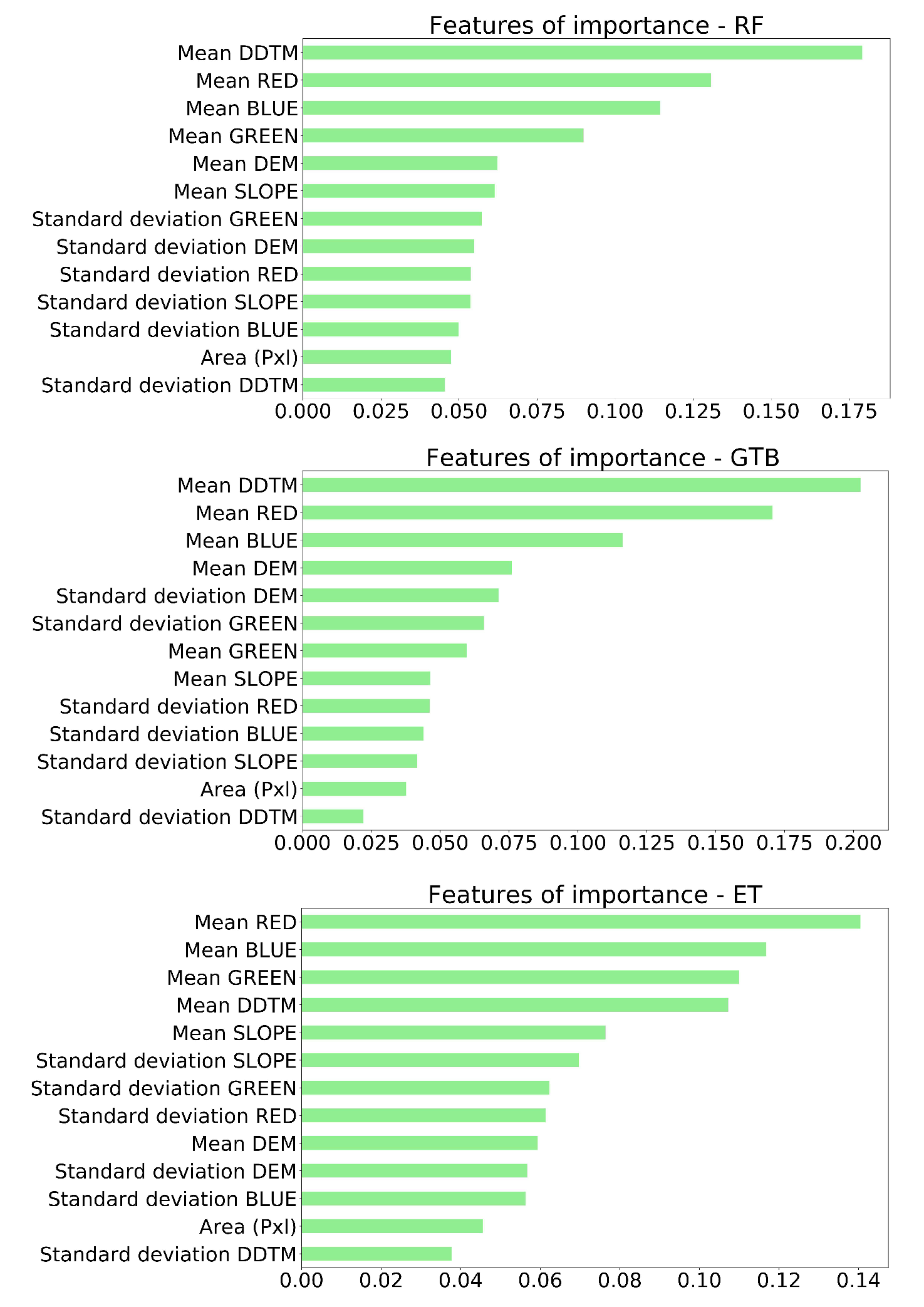
• Random forest proved to be the most efficient classifier among other well-known classifiers tested in this work: extra tree (ET), gradient tree boosting (GTB), extreme gradient boost (XGB) and voting classifier (VC);
• The detrended digital terrain model (DDTM), calculated in GIS and representing the height of floodplain pixels with respect to the water channel, proved to be the most important and required feature to classify the investigated classes;
• Almost 2 million square kilometers of the European territory were processed and mapped automatically into main riverscape units at 2.5-m spatial resolution, with a global accuracy of OA = 0.915 and per-class F1 scores of: water (W) = 0.97, sediment bars (SB) = 0.79, riparian vegetation (RV) = 0.83 and other floodplain units (OFU) = 0.93;
• The Copernicus VHR layer—although developed as a visual seamless mosaic from pan-sharpened SPOT5 data at 10-m spatial resolution, and with missing near-infrared band—still proved to be a useful layer for automated image analysis and classification if exploited in the proper way, and in combination with other sources of data;
• The produced riverscape units map at pan-European scale was a novel product not existing so far, representing a notable source of information for forthcoming studies aimed at fluvial geomorphological processes monitoring at the continental scale. If a similar mapping were applied in the future to sequential RS observations, it could be possible to generate an archive of spatial and topographical riverscape units’ characteristics, measured in an objective and quantitative way, through time and continuously along the main European river networks. Such information could help advance scientific understanding of fluvial geomorphology, while providing tools for river managers to design large-scale cost-effective rehabilitation plans and assess their effectiveness.

References

1. European Environmental Agency. European Waters: Assessment of Status and Pressures; EEA Report No 7/2018; EEA: Copenaghen, Denmark, 2018.
2. Rinaldi, M.; Surian, N.; Comiti, F.; Bussettini, M. A method for the assessment and analysis of the hydromorphological condition of Italian streams: The Morphological Quality Index (MQI). Geomorphology 2013, 180, 96–108. [Google Scholar] [CrossRef]
3. Raven, P.J.; Holmes, N.T.H.; Charrier, P.; Dawson, F.H.; Naura, M.; Boon, P.J. Towards a harmonized approach for hydromorphological assessment of rivers in Europe: A qualitative comparison of three survey methods. Aquat. Conserv. Mar. Freshw. Ecosyst. 2002, 12, 405–424. [Google Scholar] [CrossRef]
4. Carbonneau, P.; Fonstad, M.A.; Marcus, W.A.; Dugdale, S.J. Making riverscapes real. Geomorphology 2012, 137, 74–86. [Google Scholar] [CrossRef]
5. Marcus, W.A.; Fonstad, M.A. Remote sensing of rivers: The emergence of a subdiscipline in the river sciences. Earth Surf. Process. Landf. 2010, 35, 1867–1872. [Google Scholar] [CrossRef]
6. Piégay, H.; Arnaud, F.; Belletti, B.; Bertrand, M.; Bizzi, S.; Carbonneau, P.; Dufour, S.; Liébault, F.; Ruiz-Villanueva, V.; Slater, L. Remotely sensed rivers in the Anthropocene: State of the art and prospects. Earth Surf. Process. Landf. 2020, 45, 157–188. [Google Scholar] [CrossRef]
7. Belletti, B.; Dufour, S.; Piégay, H. What Is the Relative Effect of Space and Time To Explain the Braided River Width and Island Patterns At a Regional Scale? River Res. Appl. 2013, 31, 1–15. [Google Scholar] [CrossRef]
8. Marcus, W.A.; Fonstad, M.A.; Legleiter, C.J. Management Applications of Optical Remote Sensing in the Active River Channel. In Fluvial Remote Sensing for Science and Management; Carbonneau, P., Piegay, H., Eds.; John Wiley & Sons, Ltd.: Chichester, UK, 2012; pp. 19–42. [Google Scholar]
9. Ham, D.; Church, M. Channel Island and Active Channel Stability in the Lower Fraser River Gravel Reach; Department of Geography, the University of British Columbia: Vancouver, BC, Canada, 2002. [Google Scholar]
10. Gurnell, A.M.; Petts, G.E.; Hannah, D.M.; Smith, B.P.G.; Edwards, P.J.; Kollmann, J.; Ward, J.V.; Tockner, K. Riparian vegetation and island formation along the gravel—Bed Fiume Tagliamento, Italy. Earth Surf. Process. Landf. 2001, 26, 31–62. [Google Scholar] [CrossRef]
11. Spada, D.; Molinari, P.; Bertoldi, W.; Vitti, A.; Zolezzi, G. Multi-Temporal Image Analysis for Fluvial Morphological Characterization with Application to Albanian Rivers. ISPRS Int. J. Geo Inf. 2018, 7, 314. [Google Scholar] [CrossRef] [Green Version]
12. Jones, J.; Börger, L.; Tummers, J.; Jones, P.; Lucas, M.; Kerr, J.; Kemp, P.; Bizzi, S.; Consuegra, S.; Marcello, L.; et al. A comprehensive assessment of stream fragmentation in Great Britain. Sci. Total Environ. 2019, 673, 756–762. [Google Scholar] [CrossRef] [Green Version]
13. Grizzetti, B.; Pistocchi, A.; Liquete, C.; Udias, A.; Bouraoui, F.; Van De Bund, W. Human pressures and ecological status of European rivers. Sci. Rep. 2017, 7, 205. [Google Scholar] [CrossRef] [Green Version]
14. Fehér, J.; Judit, G.; Kinga Szurdiné Veres András, K.; Kari, A.; Lidija, G.; Tina, K.; Monika, P.; Claudette, S.; Theo, P.; Ekaterina Laukkonen Anna-Stiina, H.; et al. Hydromorphological Alterations and Pressures in European Rivers, Lakes, Transitional and Coastal Waters; European Topic Centre on Inland, Coastal and Marine Waters: Prague, Czech Republic, 2012; Volume 2. [Google Scholar]
15. Bertrand, M.; Piégay, H.; Pont, D.; Liébault, F.; Sauquet, E. Sensitivity analysis of environmental changes associated with riverscape evolutions following sediment reintroduction: Geomatic approach on the Drôme River network, France. Int. J. River Basin Manag. 2013, 11, 19–32. [Google Scholar] [CrossRef]
16. Belletti, B.; Dufour, S.; Piégay, H. Regional assessment of the multi-decadal changes in braided riverscapes following large floods (Example of 12 reaches in South East of France). Adv. Geosci. 2014, 37, 57–71. [Google Scholar] [CrossRef] [Green Version]
17. Demarchi, L.; Bizzi, S.; Piégay, H. Regional hydromorphological characterization with continuous and automated remote sensing analysis based on VHR imagery and low-resolution LiDAR data. Earth Surf. Process. Landf. 2017, 42, 531–551. [Google Scholar] [CrossRef]
18. Bizzi, S.; Piégay, H.; Demarchi, L.; van de Bund, W.; Weissteiner, C.J.; Gob, F. LiDAR-based fluvial remote sensing to assess 50–100-year human-driven channel changes at a regional level: The case of the Piedmont. Earth Surf. Process. Landf. 2019, 44, 471–489. [Google Scholar] [CrossRef]
19. Lang, S.; Hay, G.J.; Baraldi, A.; Tiede, D.; Blaschke, T. Geobia Achievements and Spatial Opportunities in the Era of Big Earth Observation Data. ISPRS Int. J. Geo Inf. 2019, 8, 474. [Google Scholar] [CrossRef] [Green Version]
20. Hay, G.J.; Castilla, G. Geographic object-based image analysis (GEOBIA): A new name for a new discipline. In Lecture Notes in Geoinformation and Cartography; Blaschke, T., Lang, S., Hay, G.J., Eds.; Springer: Berlin/Heidelberg, Germany, 2008; pp. 75–89. ISBN 978-3-540-77058-9. [Google Scholar]
21. Belgiu, M.; Csillik, O. Sentinel-2 cropland mapping using pixel-based and object-based time-weighted dynamic time warping analysis. Remote Sens. Environ. 2018, 204, 509–523. [Google Scholar] [CrossRef]
22. Blaschke, T.; Hay, G.J.; Kelly, M.; Lang, S.; Hofmann, P.; Addink, E.; Queiroz Feitosa, R.; van der Meer, F.; van der Werff, H.; van Coillie, F.; et al. Geographic Object-Based Image Analysis—Towards a new paradigm. ISPRS J. Photogramm. Remote Sens. 2014, 87, 180–191. [Google Scholar] [CrossRef] [Green Version]
23. Garcia-Pedrero, A.; Gonzalo-Martin, C.; Fonseca-Luengo, D.; Lillo-Saavedra, M. A GEOBIA Methodology for Fragmented Agricultural Landscapes. Remote Sens. 2015, 7, 767–787. [Google Scholar] [CrossRef] [Green Version]
24. Liu, D.; Xia, F. Assessing object-based classification: Advantages and limitations. Remote Sens. Lett. 2010, 1, 187–194. [Google Scholar] [CrossRef]
25. Georganos, S.; Grippa, T.; Vanhuysse, S.; Lennert, M.; Shimoni, M.; Kalogirou, S.; Wolff, E. Less is more: Optimizing classification performance through feature selection in a very-high-resolution remote sensing object-based urban application. GISci. Remote Sens. 2018, 55, 221–242. [Google Scholar] [CrossRef]
26. Chen, G.; Weng, Q.; Hay, G.J.; He, Y. Geographic object-based image analysis (GEOBIA): Emerging trends and future opportunities. GISci. Remote Sens. 2018, 55, 159–182. [Google Scholar] [CrossRef]
27. Ma, L.; Li, M.; Ma, X.; Cheng, L.; Du, P.; Liu, Y. A review of supervised object-based land-cover image classification. ISPRS J. Photogramm. Remote Sens. 2017, 130, 277–293. [Google Scholar] [CrossRef]
28. Ardabili, S.; Mosavi, A.; Várkonyi-Kóczy, A.R. Advances in Machine Learning Modeling Reviewing Hybrid and Ensemble Methods. In Engineering for Sustainable Future. INTER-ACADEMIA 2019. Lecture Notes in Networks and Systems; Várkonyi-Kóczy, A., Ed.; Springer: Cham, Switzerland, 2020; pp. 215–227. [Google Scholar] [CrossRef]
29. Seni, G.; Elder, J.F. Ensemble Methods in Data Mining: Improving Accuracy Through Combining Predictions; Morgan & Claypool Publishers: Williston, ND, USA, 2010; Volume 2. [Google Scholar]
30. Onojeghuo, A.O.; Onojeghuo, A.R. Object-based habitat mapping using very high spatial resolution multispectral and hyperspectral imagery with LiDAR data. Int. J. Appl. Earth Obs. Geoinf. 2017, 59, 79–91. [Google Scholar] [CrossRef]
31. Amini, S.; Homayouni, S.; Safari, A.; Darvishsefat, A.A. Object-based classification of hyperspectral data using Random Forest algorithm. Geo Spat. Inf. Sci. 2018, 21, 127–138. [Google Scholar] [CrossRef] [Green Version]
32. Qian, Y.; Zhou, W.; Yan, J.; Li, W.; Han, L. Comparing Machine Learning Classifiers for Object-Based Land Cover Classification Using Very High Resolution Imagery. Remote Sens. 2014, 7, 153–168. [Google Scholar] [CrossRef]
33. Jozdani, S.E.; Johnson, B.A.; Chen, D. Comparing Deep Neural Networks, Ensemble Classifiers, and Support Vector Machine Algorithms for Object-Based Urban Land Use/Land Cover Classification. Remote Sens. 2019, 11, 1713. [Google Scholar] [CrossRef] [Green Version]
34. Demarchi, L.; Bizzi, S.; Piégay, H. Hierarchical Object-Based Mapping of Riverscape Units and in-Stream Mesohabitats Using LiDAR and VHR Imagery. Remote Sens. 2016, 8, 97. [Google Scholar] [CrossRef] [Green Version]
35. Shen, H.; Lin, Y.; Tian, Q.; Xu, K.; Jiao, J. A comparison of multiple classifier combinations using different voting-weights for remote sensing image classification. Int. J. Remote Sens. 2018, 39, 3705–3722. [Google Scholar] [CrossRef]
36. Vogt, J.; Soille, P.; De Jager, A.; Rimavičiūtė, E.; Mehl, W.; Foisneau, S.; Bódis, K.; Dusart, J.; Paracchini, M.L.; Haastrup, P.; et al. A Pan-European River and Catchment Database; OPOCE: Luxembourg, 2007. [Google Scholar]
37. Copernicus Land Monitoring Services Very High Resolution Image Mosaic 2012—True Colour (2.5 m). Available online: https://land.copernicus.eu/imagery-in-situ/european-image-mosaics/very-high-resolution/vhr-2012?tab=metadata (accessed on 2 March 2020).
38. European Parliament-Council of the European Union. EC Council Directive 1059/2003 on the Establishment of a Common Classification of Territorial Units for Statistics (NUTS); European Parliament-Council of the European Union: Brussel, Belgium, 2003. [Google Scholar]
39. Demarchi, L.; Canters, F.; Chan, J.C.-W.; Van de Voorde, T. Multiple Endmember Unmixing of CHRIS/Proba Imagery for Mapping Impervious Surfaces in Urban and Suburban Environments. IEEE Trans. Geosci. Remote Sens. 2012, 50, 3409–3424. [Google Scholar] [CrossRef]
40. Weng, Q. Remote sensing of impervious surfaces in the urban areas: Requirements, methods, and trends. Remote Sens. Environ. 2012, 117, 34–49. [Google Scholar] [CrossRef]
41. Roux, C.; Alber, A.; Bertrand, M.; Vaudor, L.; Piégay, H. “FluvialCorridor”: A new ArcGIS toolbox package for multiscale riverscape exploration. Geomorphology 2014, 242, 29–37. [Google Scholar] [CrossRef]
42. Alber, A.; Piégay, H. Spatial disaggregation and aggregation procedures for characterizing fluvial features at the network-scale: Application to the Rhône basin (France). Geomorphology 2011, 125, 343–360. [Google Scholar] [CrossRef]
43. Notebaert, B.; Piégay, H. Multi-scale factors controlling the pattern of floodplain width at a network scale: The case of the Rhône basin, France. Geomorphology 2013, 200, 155–171. [Google Scholar] [CrossRef]
44. Benz, U.C.; Hofmann, P.; Willhauck, G.; Lingenfelder, I.; Heynen, M. Multi-resolution, object-oriented fuzzy analysis of remote sensing data for GIS-ready information. ISPRS J. Photogramm. Remote Sens. 2004, 58, 239–258. [Google Scholar] [CrossRef]
45. Saini, R.; Ghosh, S.K. Ensemble classifiers in remote sensing: A review. In Proceedings of the International Conference on Computing, Communication and Automation (ICCCA), Greater Noida, India, 5–6 May 2017; IEEE: Greater Noida, India, 2017. [Google Scholar]
46. Briem, G.J.; Benediktsson, J.A.; Sveinsson, J.R. Boosting, bagging, and consensus based classification of multisource remote sensing data. In Multiple Classifier Systems. MCS 2001. Lecture Notes in Computer Science; Kittler, J., Roli, F., Eds.; Springer: Berlin/Heidelberg, Germany, 2001; Volume 2096, pp. 279–288. ISBN 3540422846. [Google Scholar]
47. Ghimire, B.; Rogan, J.; Galiano, V.; Panday, P.; Neeti, N. An evaluation of bagging, boosting, and random forests for land-cover classification in Cape Cod, Massachusetts, USA. GISci. Remote Sens. 2012, 49, 623–643. [Google Scholar] [CrossRef]
48. Hastie, T.; Tibshirani, R.; Friedman, J. The Elements of Statistical Learning. Data Mining, Inference, and Prediction, 2nd ed.; Springer Series in Statistics, Verlag: New York, NY, USA, 2009. [Google Scholar]
49. Breiman, L. Bagging predictors. Mach. Learn. 1996, 24, 123–140. [Google Scholar] [CrossRef] [Green Version]
50. Ho, T.K. A data complexity analysis of comparative advantages of decision forest constructors. Pattern Anal. Appl. 2002, 5, 102–112. [Google Scholar] [CrossRef]
51. Belgiu, M.; Drăgu, L. Random forest in remote sensing: A review of applications and future directions. ISPRS J. Photogramm. Remote Sens. 2016, 114, 24–31. [Google Scholar] [CrossRef]
52. Chan, J.C.W.; Paelinckx, D. Evaluation of Random Forest and Adaboost tree-based ensemble classification and spectral band selection for ecotope mapping using airborne hyperspectral imagery. Remote Sens. Environ. 2008, 112, 2999–3011. [Google Scholar] [CrossRef]
53. Pal, M. Random forest classifier for remote sensing classification. Int. J. Remote Sens. 2005, 26, 217–222. [Google Scholar] [CrossRef]
54. Tian, S.; Zhang, X.; Tian, J.; Sun, Q. Random Forest Classification of Wetland Landcovers from Multi-Sensor Data in the Arid Region of Xinjiang, China. Remote Sens. 2016, 8, 954. [Google Scholar] [CrossRef] [Green Version]
55. Abdel-Rahman, E.M.; Ahmed, F.B.; Ismail, R. Random forest regression and spectral band selection for estimating sugarcane leaf nitrogen concentration using EO-1 Hyperion hyperspectral data. Int. J. Remote Sens. 2013, 34, 712–728. [Google Scholar] [CrossRef]
56. Geurts, P.; Ernst, D.; Wehenkel, L. Extremely randomized trees. Mach. Learn. 2006, 63, 3–42. [Google Scholar] [CrossRef] [Green Version]
57. Breiman, L. Arcing classifiers. Ann. Stat. 1998, 26, 801–849. [Google Scholar] [CrossRef]
58. Schapire, R.E. The strength of weak learnability. Mach. Learn. 1990, 5, 197–227. [Google Scholar] [CrossRef] [Green Version]
59. Khairuddin, A.R.; Alwee, R.; Haron, H. A proposed gradient tree boosting with different loss function in crime forecasting and analysis. In Emerging Trends in Intelligent Computing and Informatics. IRICT 2019. Advances in Intelligent Systems and Computing; Saeed, F., Mohammed, F., Gazem, N., Eds.; Springer: Cham, Switzerland, 2020; Volume 1073, pp. 189–198. [Google Scholar]
60. Boschetti, A.; Massaron, L. Python Data Science Essentials; Packt Publishing Limited: Birmingham, UK, 2015; ISBN 9780874216561. [Google Scholar]
61. Friedman, J.H. Greedy function approximation: A gradient boosting machine. Ann. Stat. 2001, 29, 1189–1232. [Google Scholar] [CrossRef]
62. Georganos, S.; Grippa, T.; Vanhuysse, S.; Lennert, M.; Shimoni, M.; Wolff, E. Very High Resolution Object-Based Land Use-Land Cover Urban Classification Using Extreme Gradient Boosting. IEEE Geosci. Remote Sens. Lett. 2018, 15, 607–611. [Google Scholar] [CrossRef] [Green Version]
63. Zhang, H.; Eziz, A.; Xiao, J.; Tao, S.; Wang, S.; Tang, Z.; Zhu, J.; Fang, J. High-Resolution Vegetation Mapping Using eXtreme Gradient Boosting Based on Extensive Features. Remote Sens. 2019, 11, 1505. [Google Scholar] [CrossRef] [Green Version]
64. Ustuner, M.; Sanli, F.B.; Abdikan, S.; Bilgin, G.; Goksel, C. A Booster Analysis of Extreme Gradient Boosting for Crop Classification using PolSAR Imagery. In Proceedings of the 2019 8th International Conference on Agro-Geoinformatics, Agro-Geoinformatics 2019, Istanbul, Turkey, 16–19 July 2019; IEEE: Istanbul, Turkey, 2019. [Google Scholar]
65. Sandino, J.; Pegg, G.; Gonzalez, F.; Smith, G. Aerial Mapping of Forests Affected by Pathogens Using UAVs, Hyperspectral Sensors, and Artificial Intelligence. Sensors 2018, 18, 944. [Google Scholar] [CrossRef] [Green Version]
66. Dong, H.; Xu, X.; Wang, L.; Pu, F. Gaofen-3 PolSAR Image Classification via XGBoost and Polarimetric Spatial Information. Sensors 2018, 18, 611. [Google Scholar] [CrossRef] [Green Version]
67. Man, C.D.; Nguyen, T.T.; Bui, H.Q.; Lasko, K.; Nguyen, T.N.T. Improvement of land-cover classification over frequently cloud-covered areas using Landsat 8 time-series composites and an ensemble of supervised classifiers. Int. J. Remote Sens. 2018, 39, 1243–1255. [Google Scholar] [CrossRef]
68. Pedregosa, F.; Varoquaux, G.; Gramfort, A.; Michel, V.; Thirion, B.; Grisel, O.; Blondel, M.; Prettenhofer, P.; Weiss, R.; Dubourg, V.; et al. Scikit-learn: Machine learning in Python. J. Mach. Learn. Res. 2011, 12, 2825–2830. [Google Scholar]
69. Radoux, J.; Bogaert, P. Accounting for the area of polygon sampling units for the prediction of primary accuracy assessment indices. Remote Sens. Environ. 2014, 142, 9–19. [Google Scholar] [CrossRef]
70. Andrade, C. The P value and statistical significance: Misunderstandings, explanations, challenges, and alternatives. Indian J. Psychol. Med. 2019, 41, 210–215. [Google Scholar] [CrossRef]
71. Buffington, J.M.; Montgomery, D.R. Geomorphic classification of river. In Treatise on Geomorphology; Shroder, J., Wohl, E., Eds.; Academic Press: San Diego, CA, USA, 2013; pp. 730–767. [Google Scholar]
Figure 1. Copernicus very high resolution (VHR) mosaic with selected catchment characterization model (CCM2) zones in this work. Selected image tiles used in the processing in this paper are drawn as black light boxes.
Remotesensing 12 01222 g001
Figure 2. The Digital Elevation Model over Europe (EU-DEM) (25-m resolution) and the selected river segments analyzed in this work (red).
Remotesensing 12 01222 g002
Figure 3. Some examples of the variable river types and forms analyzed in this study.
Remotesensing 12 01222 g003
Figure 4. Different sources of data used and flowchart of the processing.
Remotesensing 12 01222 g004
Figure 5. Example of the “Fluvial corridor” toolbox results: VB (blue) and river segments (red) shapefiles overlaid on Copernicus VHR mosaic (left) and DDTM layer (right).
Remotesensing 12 01222 g005
Figure 6. Valley bottom results for each zone analyzed. Randomly selected tiles where collection of training and validation samples was performed are also plotted in green boxes.
Remotesensing 12 01222 g006
Figure 7. Example of the obtained GEOBIA segmentation along different river sections.
Remotesensing 12 01222 g007
Figure 8. Example of reference samples collection with random spatial distribution.
Remotesensing 12 01222 g008
Figure 9. Overall accuracy (OA) comparison obtained from the different Ensemble classifiers. p-values resulting from the t-test comparisons are displayed. Black triangles represent the mean OA values (also written).
Remotesensing 12 01222 g009
Figure 10. Features of importance for RF, GTB and ET respectively.
Remotesensing 12 01222 g010
Figure 11. Normalized confusion matrices for the point-base validation of the RF riverscape units map, zone by zone and global assessment. Corresponding class codes are reported in Table 3.
Remotesensing 12 01222 g011
Figure 12. Normalized confusion matrices for the area-base validation of the RF riverscape units map, zone by zone and global assessment. Corresponding class codes are reported in Table 3.
Remotesensing 12 01222 g012
Figure 13. OA values for the point-based and area-based assessment methods per zone of analysis.
Remotesensing 12 01222 g013
Figure 14. Per-class producer accuracy (PA) values for the point-based and area-based assessments divided by zone of analysis.
Remotesensing 12 01222 g014
Figure 15. Global per-class F1 scores for the point-based and area-based assessments.
Remotesensing 12 01222 g015
Figure 16. Examples of the classification map for different river types found around Europe.
Remotesensing 12 01222 g016