Round Robin Assessment of Radar Altimeter Low Resolution Mode and Delay-Doppler Retracking Algorithms for Significant Wave Height

Abstract

Radar altimeters have been measuring ocean significant wave height for more than three decades, with their data used to record the severity of storms, the mixing of surface waters and the potential threats to offshore structures and low-lying land, and to improve operational wave forecasting. Understanding climate change and long-term planning for enhanced storm and flooding hazards are imposing more stringent requirements on the robustness, precision, and accuracy of the estimates than have hitherto been needed. Taking advantage of novel retracking algorithms, particularly developed for the coastal zone, the present work aims at establishing an objective baseline processing chain for wave height retrieval that can be adapted to all satellite missions. In order to determine the best performing retracking algorithm for both Low Resolution Mode and Delay-Doppler altimetry, an objective assessment is conducted in the framework of the European Space Agency Sea State Climate Change Initiative project. All algorithms process the same Level-1 input dataset covering a time-period of up to two years. As a reference for validation, an ERA5-based hindcast wave model as well as an in-situ buoy dataset from the Copernicus Marine Environment Monitoring Service In Situ Thematic Centre database are used. Five different metrics are evaluated: percentage and types of outliers, level of measurement noise, wave spectral variability, comparison against wave models, and comparison against in-situ data. The metrics are evaluated as a function of the distance to the nearest coast and the sea state. The results of the assessment show that all novel retracking algorithms perform better in the majority of the metrics than the baseline algorithms currently used for operational generation of the products. Nevertheless, the performance of the retrackers strongly differ depending on the coastal proximity and the sea state. Some retrackers show high correlations with the wave models and in-situ data but significantly under- or overestimate large-scale spectral variability. We propose a weighting scheme to select the most suitable retrackers for the Sea State Climate Change Initiative programme.

1. Introduction

Space-borne radar altimetry has been a remote sensing approach for many decades. The satellite altimeter adopts a simple principle, as already been described in 1979 by [1]: it emits a short radio-wave pulse and detects the reflected echo from the Earth’s surface. From the round-trip time the pulse takes, the distance between the satellite’s instrument and the Earth can be estimated. Initially, satellite altimetry over the ocean was used for measuring the ocean surface topography, but it can exploit other properties of the received echoes for retrieving significant wave height (SWH) and wind speed (WS). The SWH is defined as four times the standard deviation (SD) of the sea surface elevation [2]. Acquiring a global knowledge about the oceans’ SWH is essential for applications such as ocean wave monitoring (e.g., for the fishing industry, industrial shipping route planning), weather forecasting, or wave climate studies (e.g., [3]).

Brown and Hayne have developed, in 1977, 1980 an open-ocean altimeter waveform model (in the following referred to as the Brown-Hayne (BH) model), with which the SWH can be inferred from the slope of the leading edge of the received echo [4,5]. The key part of the waveform that responds to changes in SWH is the leading edge. As the unwanted extraneous returns in the coastal zone predominantly affect the trailing edge, a whole class of retracking algorithms has been recently developed that focuses on the “subwaveform”, i.e., those waveform bins centred around the leading edge. Altimeters that continuously emit and receive pulses in an alternating manner with a pulse repetition frequency (PRF) of 1920 Hz yield a footprint size of around 7 km and are referred to as pulse-limited, Low Resolution Mode (LRM) altimeters. In contrast, the more recent Delay-Doppler altimetry (DDA) altimeters (synthetic aperture radar (SAR) altimeters and synthetic aperture radar mode (SARM) are equivalent terms) transmit bursts of pulses (64 for the Sentinel-3 (S3) altimeters) and make use of both time delay and Doppler shifts of the echoes, resulting in a much narrower footprint and an increased along-track resolution of about 300 m. The appropriate physical-based waveform model for DDA is the SAMOSA model, which was developed in the framework of the European Space Agency (ESA) SAR Altimetry MOde Studies and Applications (SAMOSA) project [6] and published in [7]. The term SAMOSA is also used to refer to the actual retracking algorithm, as documented in [8].

Retracking is the common process of extraction of the geophysical parameters from the received echo and is performed using an algorithmic approach. The authors of [9] categorised three different main types of retracking algorithms. Empirical retrackers are based on a heuristic approach, in which an empirical-based relationship is established between the waveform and the geophysical quantities. The approach of physical-based retrackers is to fit the waveform to an idealised mathematical model. In its most accurate form, the model is a numerical-based solution and mimics the processing chain and physical effects (e.g., the interaction of the pulse with the Earth’s surface) as close as possible. The closed-form analytical (or semi-analytical) solution of a physical-based retracker meets certain simplifying assumptions, which makes the computation of the model more robust, versatile, and computationally less expensive. The third category of retrackers uses a statistical approach, which makes use of statistical information of neighbouring measurements.

The focus of this work is an objective assessment of the performance of different retracking algorithms with regards to the estimation of the SWH in dependence of the distance-to-coast (dist2coast) and the sea state.

When estimating the SWH using satellite altimetry, the following main limitations can be identified:

• The contamination of the spurious signal components in the coastal zone results in a deteriorated quality and reduced quantity of SWH estimations [10]. The interfering signals mostly arise from “mirror”-like surfaces, such as melt ponds on sea-ice, or in sheltered bays, [11,12,13]. These phenomena are similar to the so-called “sigma0-blooms” in the open-ocean [14] but affect significantly more data in the coastal zone.
• The power spectral density (PSD) estimate of the SWH, which is computed as a function of spatial wavelength and denoted as the wave spectral variability, is characterised by a so-called “spectral hump” that masks the along-track variability below 100 km [14].
• The precision of the estimation of extreme sea states is particularly poor [15].
• Very low sea states cause the leading edge of the returned echo to be very steep, implying that that part is only sampled by one or two waveforms gates. Consequently, the precision is also degraded in low sea states [16].

The assessment is part of the Round Robin (RR) exercise that is conducted in the framework of the Sea State Climate Change Initiative (SeaState_cci) of ESA [17], launched in June 2018. The main objective of the project is the estimation and the exploitation of consistent climate-quality time-series of SWH across different satellite missions.

For conducting the RR assessment, we determined beforehand the set of rules on how the evaluation was to be performed and what performance metrics were to be extracted. The exercise of a RR constitutes an essential part of the development phase of an ESA Climate Change Initiative (CCI) Essential Climate Variable (ECV) project [18]. It is open to both internal and external participants and its general procedure is as follows. A data package containing satellite data, and auxiliary data is distributed among all involved parties. The participants apply their algorithms to the data and send back their output. The pre-agreed assessment metrics are extracted from the generated datasets and the best performing algorithm is selected. The Sea Surface Temperature Climate Change Initiative (SST_cci) [19], Soil Moisture Climate Change Initiative (SoilMoisture_cci) [20], and Ocean Colour Climate Change Initiative (OC_cci) [21] projects are examples of other projects, in which RRs were performed.

Ardhuin et al. [15] have elaborated on the requirements, the existing measurement technologies, and their limitations and the future of how sea states can be observed. Regarding the estimation of the SWH data from altimetry, most of the studies limit the comparison to only a single retracker against external data, or to a new retracker compared to the existing product. The authors of [10] have validated the Adaptive Leading Edge Subwaveform (ALES) algorithm using LRM altimetry for SWH estimation in the coastal zone. The result was validated against in-situ data by assessing bias, SD, slope of regression line, and number of cycles with correlation larger than 0.9. The authors of [22] and [23] have assessed the SWH and WS estimates that were acquired by the missions SARAL/AltiKa and CryoSat-2 (CS2) using the standard retracking algorithms MLE-4 and SAMOSA, while comparing the measurements against in-situ buoy data and wave models. The ESA SAR Altimetry Coastal and Open Ocean Performance (SCOOP) project [24] has conducted the characterisation and improvement of DDA retracking algorithms. The involved teams have made improvements on the retrackers and have assessed the resulting performance in comparison against the baseline algorithms but not against several other retrackers. Yang and Zhang [25] have validated the baseline retrackers SAMOSA and MLE-4 of Sentinel-3A/3B (S3A/B) datasets against open-ocean buoy data of the U.S. National Data Buoy Center (NDBC) network, whilst Nencioli and Quartly [26] have performed a detailed analysis of the same using both models and buoys around the southwest UK. Fenoglio-Marc et al. [27] have validated the performance of the standard SAMOSA retracker from the CS2 mission in the study area of the German Bight. The authors of [28] and [9] have presented a novel SAMOSA+ and SAMOSA++ retracker, while validating their results with in-situ and wave model data.

To the best knowledge of the authors, there has not been any comparable objective and comprehensive comparison between different retracking algorithms in the literature so far. In this pioneering RR exercise for SWH, we have endeavoured to use multi-year quasi-global datasets. However, to prevent an undue load on the various data producers, they were only required to process a selection of tracks spanning the range of conditions to be assessed (see

Table 1. Summary of J3 and S3A input L1 datasets to be retracked.

	Mission	Jason-3	Sentinel-3A
# of
Half-orbits/pole-to-pole tracks		16	30
Cycles		73	17
Period of time in months		24	15
NetCDF files (pole-pole tracks and cycles)		1162	512

). In this work, a compromise had to be found between the need to cover several regions of the world, the amount of data for a statistically-meaningful comparison, and the fact that most of the participating algorithms are not yet associated to an already available global product. A strict time line was set for the participants in order to process the specific set of data. Further discussion can be found in Section 2.

This work is structured as follows: Section 2 describes the data that were used for the assessment of the algorithms, including the Level-1 (L1) input datasets used for retracking, a brief description of the retracking algorithms and also the wave models and the in-situ data used in the validation. Section 3 describes the methodology of the assessment, explaining how the evaluation metrics are extracted and the design of the software framework that is used for the automatic generation of the results. Section 4 presents and discusses the results. Section 5 discusses some lessons that were learnt during the process and should be applied to future RRs. Section 6 draws conclusions and elaborates on the algorithm selection process of the SeaState_cci consortium.

2. Data

2.1. Original Altimeter Data

In order to conduct an objective evaluation of different retracking algorithms, it is crucial that all algorithms process exactly the same data. It was therefore decided that the input for all providers should be the same L1 along-track data from Sentinel-3A (S3A) and Janson-3 (J3).

The selected J3 dataset is the Sensor Geophysical Data Records (SGDR) version D product that was downloaded from Aviso+ [29]. It contains both the radar waveforms and also SWH estimates generated with the baseline algorithms MLE-3 and MLE-4; these default retrackers are also included in the assessment to provide a benchmark. The time period being used was from the 1st of June 2016 to 30th of June 2018 in order to capture a wide range of sea state conditions.

For S3A, we used Level-1A (L1A)/Level-1B with stack data (L1BS) data acquired from the Copernicus Online Data Access (CODA) catalogue of EUMETSAT [30]. The files cover a time period from 26th of March 2017 to the 30th of June 2018. In contrast to the J3 SGDR dataset files, the geophysical data and standard retracking estimates are not contained in the L1BS files but in the Level-2 (L2) products. For S3A, the default retracking algorithms are SAMOSA for the DDA waveforms and MLE-4-PLRM for the Pseudo Low Resolution Mode (PLRM) ones (see the end of this section for a more detailed description of the latter). To enable these two default algorithms to provide benchmarks, we collocated the needed L2 information with the L1BS locations used by all the developers of new products. The SAMOSA-retracked product that is included in the L2 product has the baseline versions 002 and 003. We had to accept two mixed baseline versions because there was a transition within the investigated period of time.

The individual pole-to-pole tracks of the J3 and S3A missions were selected to maximise the number of in-situ collocations that were used for validation of the retracked datasets, as described in Section 2.2. A summary of the input L1 datasets are listed in Table 1.

2.2. Validation Data

In-situ data were gathered by ECMWF. Most of the data came from the operational archive from ECMWF, where all data distributed via the Global Telecommunication System (GTS) are kept. Data from moored buoys and fixed platforms were extracted. These data are usually reported hourly (or less frequently). The bulk of the data comes from moored buoys, with the exception of data from operating platforms in the North and Norwegian Seas and the Gulf of Mexico. The main data providers are the US, via the NDBC and Scripps, Canada, the UK, France, Ireland, Norway, Iceland, Germany, Spain, Brazil, South Korea, and India. This dataset was supplemented by buoy data obtained from the web sites from the UK Centre for Environment, Fisheries and Aquaculture Science (CEFAS) and the Faeroe Islands network. In addition, buoy data from New-Zealand obtained as part of ECMWF wave forecast validation project were also used. A basic quality control was applied to each hourly time series for each location to remove spurious outliers. The number of buoys selected for the in-situ datasets is given in

Table 2. Number of the selected total, open-ocean and coastal buoys for the J3 and S3A missions.

	Mission	Jason-3	Sentinel-3A
# of
Open-ocean		85	124
Coastal zone		40	46
Total		125	170

. Overall nearly 36% more buoys are available for the S3A dataset than for J3 because more different tracks are used. Most of these buoys are located in the open-ocean, as shown in the map in Figure 1.

To validate the retracker results, a dataset of collocated remote sensing and in-situ observations was created based on the following constraints, as discussed in [31]: (a) the distance between the along-tracks and the buoys is less than 50 km and (b) the time difference between the along-track points and the buoy record is less than 30 min. If both constraints are satisfied during a pass-over of the satellite, the 51 measured, 20-Hz SWH points that are located closest to the buoy position are extracted and the median value is computed. The odd number of 51 is chosen for the sake of symmetry. The buoy data is smoothed by applying a 1 h moving average filter.

Besides the in-situ buoy data, a novel wave model from European Centre for Medium-Range Weather Forecasts (ECMWF) is used as a reference for the retracker validation. It is a wave hindcast, which is based on ERA5-forcing and CY46R1 version of the ECMWF wave model (referred to as ERA5-h model in the following). The original ERA5 uses ECMWF’s Integrated Forecasting System (IFS) cycle 41r2 and thus benefits from multiple decades of experience in terms of model physics, numerics, and data assimilation [32]. ERA5-h adopts the newer IFS cycle 46r1 and was found to be of even better quality than compared with ERA5 [33]. The crucial difference between both is the fact that no wave data assimilation is performed for ERA5-h as compared with ERA5, for which available space-borne altimetry data is used. ERA5-h is a wave model standalone run that is forced by ERA5 hourly 10 m neutral winds, surface air density, gustiness, and sea-ice cover. It uses different wave physics for wind input and dissipation [34]. It provides hourly estimates for a large number of ECVs. With respect to wave heights and spectra, ERA5-h has an improved resolution of 18 km, 36 directions, and 36 frequencies, as compared to ERA5 with a resolution of 40 km, 24 wave directions, and 30 frequencies.

2.3. Overview of Investigated Retracker Datasets

In total, there are 15 new retracked L2 datasets from six research groups (Technical University of Munich (TUM), Plymouth Marine Laboratory (PML), Collecte Localisation Satellites (CLS) in cooperation with the Centre national d’études spatiales (CNES), University of Bonn (UniBonn), isardSAT, University of Newcastle (UON)) incorporated in the assessment. As listed in

Table 3. Investigated Low Resolution Mode (LRM) and DDA retracking algorithms.

	Retracking Algorithms	Altimeter Mode	Author	Denoised
J3	MLE-3 (reference)	LRM	-	No
	MLE-4 (reference)	LRM	-	No
	WHALES	LRM	TUM	No
	WHALES_adj	LRM	PML/TUM	Yes
	WHALES_realPTR	LRM	PML/TUM	No
	WHALES_realPTR_adj	LRM	PML/TUM	Yes
	Brown-Peaky	LRM	UON	No
	TALES	LRM	UniBonn	No
	Adaptive	LRM	CLS/CNES	No
	Adaptive_HFA	LRM	CLS/CNES	Yes
	STARv2	LRM	UniBonn	Yes (inherently)
			Total Number	11
S3A	SAMOSA (reference)	DDA	SAMOSA project [6]	No
	WHALES-SAR	DDA	TUM	No
	DeDop-Waver	DDA	isardSAT	No
	LR-RMC	DDA	CLS/CNES	No
	LR-RMC_HFA	DDA	CLS/CNES	Yes
	MLE-4-PLRM (reference)	PLRM	-	No
	TALES-PLRM	PLRM	UniBonn	No
	STARv2-PLRM	PLRM	UniBonn	Yes (inherently)
			Total Number	8

, the number of J3 retracking algorithms is 11 (all LRM, including the baseline products MLE-3 and MLE-4) and eight for S3A (including the baseline SAMOSA product, and with three being PLRM datasets).

The column “Denoised” in Table 3 indicates whether a denoising technique was applied to the retracked dataset in order to decrease the noise content in the along-track SWH series. This could have been applied either implicitly within the retracking algorithms as for the STARv2 algorithm (as discussed in Section 2) or explicitly, a-posteriori to the retracked L2 dataset. Examples for explicit techniques are the intra-1-Hz adjustment [35] or high-frequency adjustment (HFA) [36], and an empirical mode decomposition (EMD)-based technique [37].

Rules for the RR also required that the data producer supply a quality flag to indicate whether the proponents rated the individual estimates as good (0) or bad (1).

In the following sections, the retracking algorithms, which participated in the RR, are briefly described. Where a peer-reviewed publication exists, we provide the citation. Otherwise, an extensive description of the algorithms can be found in [38]. While the focus of the paper is on the ensemble of statistics adopted to highlight differences among the retrackers, it is important to highlight the basic characteristics of the algorithms in order to be able to discuss the different performances.

2.3.1. LRM Retracking Algorithms

The established algorithm applied on the vast majority of LRM altimetry missions is named MLE-3: this maximum likelihood estimator uses the analytical BH model for retrieving the three parameters range, SWH, and signal amplitude. It was superseded by MLE-4 [39], which also allows for instrument mispointing. MLE-3 and MLE-4 actually implement an unweighted least squares (LS) fit of the analytical model to the observational data, while neglecting the expected statistics of the fading noise contribution. However, a simple weighted scheme exhibits greater along-track variability, with the introduction of correlated errors between range and SWH estimations [40].

The mathematical form, such as the BH model, assumes that the shape of the emitted radar pulse corresponds to a Gaussian and that the reflecting surface is homogeneous within the irradiated footprint, which can be between 2 and 20 km in diameter depending upon conditions [41]. First of all, the true pulse shape does not conform exactly to the ideal, so a facsimile of the emitted pulse is recorded internally, known as the Point Target Response (PTR), which can be used to develop an instrumental correction. Second, the assumption of homogeneity in the footprint often breaks down for winds speeds lower than 3 m/s and in the coastal zone because of reflections from nearby land or “bright target” responses from sheltered bays [12,13]; therefore new algorithms have been advocated to overcome these problems.

Passaro et al. [42] developed the ALES retracker to utilise only waveform bins around the leading edge, with the selection of bins being dependent upon the SWH estimate from an initial pass. Although originally developed to improve estimates of range in the coastal zone, it was also demonstrated to give more robust estimates of SWH in the German Bight [10]. The fitting of the received echo to the idealised BH model is established using the Nelder-Mead optimisation approach, which is a computational efficient algorithm for solving non-linear optimisation problems [43]. The WHALES algorithm is an improved version of ALES, in which the derivation of wave height has been optimised by developing a set of adapting weights in the fitting process, which changes according to a first estimation of the SWH performed based on the leading edge.

The standard WHALES algorithm makes a correction for the true PTR shape using a look-up table (LUT)-based on that used for MLE-4 output. A bespoke correction for WHALES was developed by running a series of simulations using a representation of the true PTR shape and examining the mean bias recorded by the WHALES algorithm assuming a standard Gaussian PTR. At wave heights greater than a few metres, this correction was uniform and similar to that from the MLE-4 LUT; however, at low SWH, especially < 0.8 m, the derived correction varied markedly with the position of the leading edge. With the correction applied as a function of wave height and leading edge position, the algorithm is referred to as WHALES_realPTR.

The above-described algorithms treat each waveform completely independently. However, as both wave height and range are derived predominantly from the waveform bins within the leading edge, they both exhibit sensitivity to the individual realisations of fading noise in that span of the waveform. In practice, the fading noise-related anomalies between the two are significantly correlated [40], with an error in range of a few centimetres being typically associated with a commensurate error in SWH of ten times that magnitude, although the coefficient of proportionality does depend upon the particular retracker and altimeter [35]. Thus, if the noise-related error in range can be ascertained, for example, by use of a high-pass filter (HPF), an appropriate adjustment of the SWH can be calculated. Such a correction was available for the WHALES retracker, producing algorithms WHALES_adj and WHALES_realPTR_adj for the two versions of WHALES previously introduced. The use of such adjustments was found to be very effective in making a significant reduction in small scale noise for MLE-4 applied to Jason-2, Jason-3, and AltiKa data [35].

The Brown-Peaky retracker [44] has been developed as a variation of the ALES approach, which defaults to using all waveform bins if no peaky signal is detected. If a peak is detected, the estimation of the geophysical parameters is performed using a weighted least squares (WLS) method. The range bins that are affected by the peak are thus down-weighted and their impact is mitigated. The algorithm developers have already assessed their product around the coasts of Australia [45].

TALES is another ALES-derivative developed by TU Darmstadt [28]. In contrast to the original ALES [46], TALES uses a numerical waveform model called Signal Model Involving Numerical Convolution (SINC) instead of the BH model [47]. Hence, no LUT is required for estimating the SWH. In addition, SINC can be adapted to more complex sea surface representations, such as weakly non-linear wave theory and a real PTR [38,47].

The model that is used for the Adaptive retracker is similar to the BH model. However, in contrast to classical retrackers, such as MLE-4, it does not assume a Gaussian-like PTR, which often also requires a LUT to provide minor corrections. Instead, it follows a numerical solution, where the real PTR is approximated by taking into account altimeter instrumental characterisation data such as the antenna beam pattern or the characteristic of the integrated low-pass filter (LPF). Likewise, it accounts for different surfaces of the sea such that it is able to cope with different degrees of roughness (diffuse or peaky) [38]. There was also a variant of this product, termed Adaptive_HFA, which included an additional along-track filtered correction term, based on the approach described in [36]. It is important to remark that for both the “adjusted” variants of WHALES and Adaptive, there is no smoothing or filtering of the SWH data but solely of the range of information to provide the corrections.

A significantly different approach to decrease the noise in the optimisation of the SWH estimation is version 2 of the STAR algorithm [48] (STARv2), although the BH model and a subwaveform technique are also employed. The original STAR algorithm has been applied to both LRM and PLRM altimetry data. STAR follows a traditional Maximum Likelihood Estimation (MLE) approach that retracks all detected subwaveforms. This yields a point cloud of values containing sea surface height (SSH), SWH, and ${\sigma }^0$. To determine the final values of SSH, SWH, and ${\sigma }^0$, a shortest path algorithm was used [48]. This is based on the assumption that neighbouring 20-Hz measurements are similar to each other. The STARv2 retracker incorporates an additional weighting factor into the selection of the individual steps from one 20-Hz measurement position to the next, which also reduces the appearance of measurement noise as along-track variability.

2.3.2. DDA Retracking Algorithms

Whilst the majority of altimetry missions launched to date have been LRM altimeters, the latest generation exploit the phase coherence of bursts of individual echoes sent at a much higher pulse repetition frequency, in a technique, referred to as DDA or also known as SAR altimetry [49]. By application of SAR-like processing, better localisation can be achieved of the part of the ocean generating the echo, and these echoes can be combined over a wider range of views (“multi-looking”) to help improve the signal-to-noise ratio (SNR). The first instrument to offer DDA mode was CS2 (launched in 2010), and this was followed by S3A/Sentinel-3B (S3B) in 2016 and 2018, respectively.

SAMOSA is the baseline retracking algorithm that is part of the standard L2 product of the EUMETSAT CODA. (Strictly speaking, the term SAMOSA is related to the ESA project [6], in which the waveform model and the retracker were developed [8], but is commonly used to refer to the retracking algorithm on the standard products.) It uses the fully analytical, open-ocean SAMOSA2 waveform model [7] that is expressed in terms of Scaled Spherical Modified Bessel functions and includes the zero- and first-order terms, as described in [28]. To establish the non-linear fitting of curves, it uses the bounded Levenberg-Marquardt Least-Squares Estimation Method (LEVMAR-LSE) [50] algorithm (as an implementation for the Levenberg-Marquardt non-linear LS optimisation algorithm) to extract the three geophysical parameters range, SWH, and amplitude $P_u$.

WHALES-SAR is the DDA counterpart of WHALES. Similarly, WHALES-SAR only considers a subwaveform and thus avoids spurious backscattered signals in the trailing edge of the waveform that mostly arise in the coastal zone and applies a weighted estimation. However, instead of being based on a physical-based retracker, it exploits the estimation of the rising time of the leading edge, which is performed using a simplified BH model with a different trailing edge slope. It, therefore, infers the SWH by means of an empirical relation that is based on a comparison with simulated DDA waveforms [38,51].

The DeDop-Waver retracker provided by isardSAT starts the processing from the L1A data, incorporating several instrumental and DDA-specific corrections. The essential retracking step is performed by following the original SAMOSA model [7] with additional steps, such as noise floor estimation, stack modelling, stack masking, and multi-looking. [52]

The L1A-to-L1BS processing of the Low Resolution with Range Migration Correction (LR-RMC) retracker follows the unfocused SAR altimetry approach from [53] with the difference that bursts of four beams are combined and averaged. Thus, it improves the measurement precision compared to unfocused SAR altimetry over open-ocean [38]. The retracking procedure to convert the L1BS to a L2 dataset is established by a numerical approach. In contrast to a conventional retracker, it uses pre-simulated power echo models that are based on altimeter instrumental characterisation data such as the real antenna pattern and the range impulse response, which were measured pre-launch, and also it takes into account instrumental ageing issues. For fitting the waveform to the model, a WLS estimator that is derived from a MLE is used. [38]

Same as for the Adaptive LRM retracker, as described in Section 2.3.1, a second variant LR-RMC_HFA is taken into consideration, which includes an additional smoothing step using the HFA algorithm [36].

These algorithms for DDA processing make use of the time delay and Doppler shift information that is contained in the return echo, whereas their forerunners only used the information binned in terms of delay. Although the extra information in the Delay-Doppler (DD) processing has been expected to give improved accuracy, there were concerns for climate studies about whether the derived values would be consistent with those from conventional LRM altimeters. Thus, for S3, there is a parallel processing line that ignores the delay information to produce PLRM waveforms. The shape of these waveforms will match the BH model, but the noise level in the waveforms is higher than for a conventional LRM instrument operating continuously, owing to the lower number of independent returns being averaged. For continuity, the S3A L2 products contain these PLRM waveforms and estimates of range, SWH and ${\sigma }^0$ based on them (denoted as MLE-4-PLRM in the following). The providers of TALES and STARv2 also applied their retracking approaches to these waveforms, and these are also evaluated to provide a yardstick, with which to assess whether DDA algorithms provide the anticipated benefits. In the following analysis, we add the suffix ’-PLRM’ to their names to clearly distinguish their source.

3. Methodology

In order to objectively assess the performance of the individual retracking algorithms, the following five different types of analyses were evaluated: outliers, noise, wave spectral variability, and the comparison against a wave model and against in-situ data. All metrics from the analyses are generated as a function of the dist2coast and the sea state. The terms coastal and open-ocean are used for dist2coast values of less than or greater than 20 km, respectively, with the classification of sea states being as in

Table 4. Definition of sea states.

Sea State	SWH Range
Low	0 m < SWH < 2 m
Average	2 m < SWH < 5 m
High	SWH > 5 m
Very high	SWH > 10 m

.

3.1. Retrackval Framework

The complete analysis code is set up as a Python-3-package, retracker validation (retrackval), which is available on request. Its main objective is to make the assessment process as transparent and objective as possible. It is platform-independent, easy-to-setup (with about 10 commands), and the full algorithm validation is reproducible by running a fully-automated script.

When reading the netCDF file of the individual dataset, the SWH data variable undergoes a first quality check. The SWH value is set to not-a-number (NaN), if one of the following conditions are met:

• The SWH value is set to NaN by the retracked dataset provider;
• The quality flag is set to “bad” by the retracked dataset provider;
• The sea-ice flag is set (not used in outlier analysis and not needed in spectral analysis or buoy comparisons);
• All values around 0 m with tolerance of 1 × 10${}^{-4}$ m. This is necessary as some retrackers set the estimated SWH value to zero, when they fail, which may give a misleading perception of the confidence with the along-track noise being 0.0 m.

In order to run the analyses as a function of dist2coast, the corresponding dist2coast value of each measurement at any location is determined from a 0.01° resolution dataset from Pacific Islands Ocean Observing System (PacIOOS) [54], which has an uncertainty of up to 1 km. For some of the analyses, data were averaged from 20 Hz (300 m along-track) to 1 Hz (∼6 km), using a median of the 20 values, provided that no more than 3 were NaN. This was useful for the comparison against the wave model (as the resolution of the ERA5-h wave model is 18 km). Also in the noise analysis, the SD was calculated over groups of 20 samples.

When reducing the longitude/latitude-pair vectors, the median of the 20 20-Hz values are taken. Likewise, the median of the 20 SWH values is computed, with the additional constraint that there must exist at least 17 valid values (neither NaN, bad quality flag, nor marked as being sea-ice) of the 20 20-Hz-points. Otherwise, the resulting 1-Hz SWH is set to NaN.

3.2. Outlier Analysis

In some situations, the retracking algorithms are not able to retrieve a reasonable estimate for the SWH from the received echo. This might be due to (a) received echoes that contain strong spurious signal components, which predominantly occur in the coastal zone, (b) extremely steep and poorly defined leading edges (likely apparent in very low sea states), or (c) very noisy waveforms that are typical of echoes reflected from within storms, with very high waves and potentially intervening rain [55]. These conditions significantly reduce the number of valid retracked SWH observations. Thus, the coastal zone, very low sea states, and storms represent key situations for major improvement. This makes the outlier analysis a particularly relevant component of the RR assessment. For detecting outliers, the following three criteria are defined:

• invalid Data missing (already set to NaN) or quality flag set to ’bad’ (1).
• out_of_range If a value is out of the expected range of $[-0.25,25]$ m. (Note noisy estimations may sometimes return sub-zero values.)
• mad_factor This criterion compares the value with its 20 closest neighbours (10 before and 10 after). It is implemented using median and median absolute deviation (MAD), which are statistically robust measures. Data are discarded if they exceed median plus 3 * 1.4826 * MAD, with median and MAD calculated on 20-point sliding windows, and the factor 1.4826 converts the MAD to SD equivalent for a normal distribution [56].

If one of the criteria is applicable, the individual measurement is considered to be an outlier. The evaluated metrics are the total number of outliers and the number of outliers in the coastal zone as a function of the dist2coast, considering bands of less than 20, 10, and 5 km from the coast. This analysis is performed on the 20 Hz-data, and the total number of outliers is given by the sum of the individual outlier types excluding potential overlapping indices (one measurement might be marked by multiple types, e.g., mad_factor and out_of_range).

Furthermore, as an exception of the outlier analysis, there is no sea-ice flag considered, when reading the netCDF files. The sea-ice flag would be considered as another kind of quality flag, marking a measurement as invalid. The outlier analysis should be on estimations of SWH in the ocean and do not take into account points on surfaces, for which such estimation does not exist, such as land and sea-ice covered areas.

3.3. Noise Analysis

The intrinsic noise that is implied in the SWH sequence is defined as the standard deviation (SD) of the 20-Hz SWH data within a 1-Hz distance. This procedure is based on the assumption that the SWH measurements that were taken from an irradiated footprint of approximately 7 km (corresponding to a 1-Hz measurement) and is mostly dominated by noise [15,27]. The variations of the 20-Hz sampling points, which amounts to a distance of roughly 300 m is, thus, considered to be noise.

The following metrics are evaluated by the retrackval framework:

• Median of all noise values: as a function of dist2coast (open-ocean and coast);
• Median of all noise values: as a function of sea state and dist2coast (open-ocean and coast);
• Median noise values vs. SWH ranges with a resolution of 0.25 m.

The reduction of 20-Hz to a 1-Hz dataset containing the noise values is performed as described in Section 3.1. Likewise, the 20-Hz dataset is read and bad data is discarded accordingly, while outliers detected in the previous sections are not.

3.4. Wave Spectral Variability

The preceding section described the intrinsic and short term variability affecting the precision of successive measurements. An extension of this analysis is to explore the variability as a function of length scale, i.e., an along-track spectral analysis, as in [35,57].

The interest here is in the perspective of mapping and monitoring applications, where the finest scale information may not be immediately useful, but the interest is in the correct characterisation of the variability at scales of 25–100 km. To assess such variability, we consider successive 1024-point sections of the SWH data (corresponding to ∼300 km along-track) and determine Fourier components using the Welch periodogram method. This method applies a Hann window to the data to mitigate the effects of any discontinuity between the values at the end of each section. As the analysis is achieved using fast Fourier transform (FFT), the data must be free from any missing values. To produce sufficient spectra for averaging, we utilise any segment that has less than 5% missing data and fill in the gaps with simple linear interpolation. We also adopt the procedure of calculating the spectra from sections commencing every 512 points along-track (i.e., 50% overlap), as the Hann weighting downplays the contributions from the outer edges of each section [58]. This analysis was deliberately constrained to data that was from the open-ocean (by setting a dist2coast > 20 km), free from land, or sea-ice (flag taken from the baseline products), so that the information derived is exclusively about the wave height field of that retracker rather than being affected by other phenomena.

3.5. Comparison against Wave Model

In the subsequent analyses, the accuracy and precision of the retracked SWH estimates are to be compared by the ERA5-h wave model described in Section 2, as has been done in [22,23]. The model is a gridded product and features a resolution of 18 km. It is, thus, as acceptable to perform the co-location (using an interpolation) on the 1-Hz SWH data points (corresponding to 7 km).

The process of the comparison analysis is performed as follows:

(1)

Reducing the datasets from 20-Hz to 1-Hz;

(2)

Taking the union of the indices of both datasets considering non-NaN values only;

(3)

(Out-of-range values were already set NaN, thus discarded during the netCDF reading procedure);

(4)

Performing a linear LS regression on the two coupled series.

As a result, the following metrics are evaluated in this analysis:

• Pearson correlation coefficient;
• Slope of linear fit;
• standard deviation of differences (SDD);
• Median bias of differences;
• 2D-histogram plot.

The SDD and the median bias of differences is computed according to

$$\mathrm{SDD}=std\left(\right|{\mathrm{SWH}}_{model}-{\mathrm{SWH}}_{retracker}\left|\right)),$$

(1)

and

$$\mathrm{median}\mathrm{bias}=median({\mathrm{SWH}}_{model}-{\mathrm{SWH}}_{retracker})$$

(2)

where $std$ denotes the SD, and $|.|$ the absolute magnitude operator.

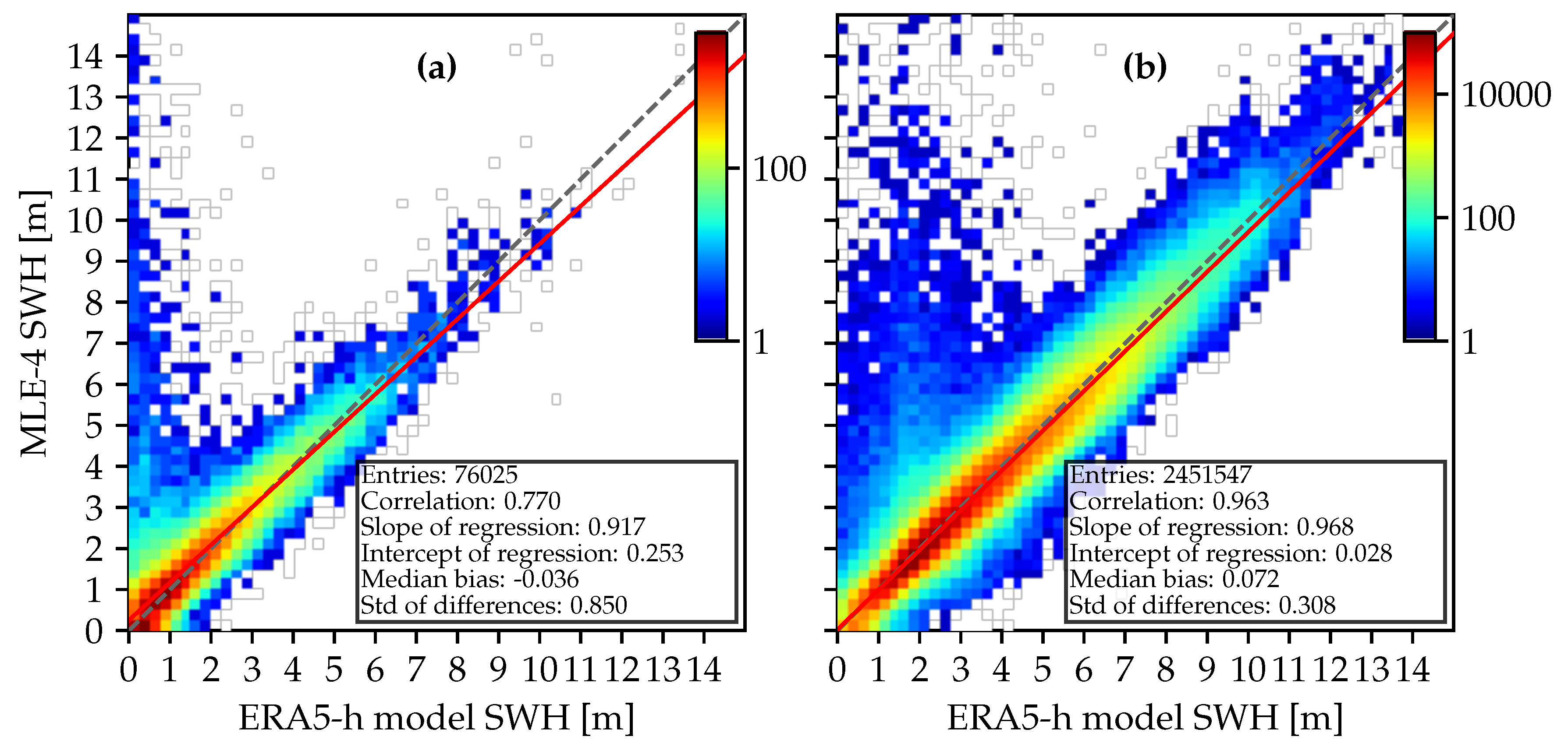
Figure 2 shows the 2D-histogram plots for the retracked MLE-4 in comparison against the ERA5-h wave model for (a) coastal and (b) open-ocean scenarios, respectively. The 2D-histogram plots are generated by assigning the two coupled datasets to SWH-intervals with a bin size of 0.25 m (taking the SWH value of the wave model as the reference). Hereby, each pair of a coupled SWH estimate corresponds to one point in the 2D-histogram. The number of the coupled estimates is colour-coded on a common logarithm-scale. The dashed line indicates a perfect correlation between the two series (correlation coefficient and slope of value 1.0). The solid red line is the result of the linear regression analysis.

When comparing Figure 2a, open-ocean and b, coastal scenarios, it can be clearly seen from the distribution of the points that there are higher sea states in open-ocean areas, as expected. The MLE-4 retracker significantly overestimates low sea states, in which the values have a large spread in these cases. This is an important remark, when discussing Figure 7 in Section 4, in which high noise values are noticeable for high sea states. There is only a minor difference between the two calculated median bias values –0.036 and 0.072 m. However, the difference of the SDDs of 0.850 and 0.308 is significant, which indicates better precision of MLE-4 for the SWH estimates in open-ocean scenarios.

The aforementioned metrics are generated by the retrackval framework for all included J3 and S3A datasets. Consequently, a large set of figures and statistical numbers are generated. Plots such as the 2D-histogram plots are convenient for a detailed analysis of the comparison against another reference dataset. In order to ease the objective assessment of the individual retrackers against a reference dataset, Section 4 will limit the evaluation to the metrics correlation coefficient, SDD and median bias of differences.

3.6. Comparison against In-Situ Data

The retracked SWH measurements are compared with the in-situ buoy records to carry out independent evaluation of accuracy and limitation of the retracking algorithms, as has been done in [22,23]. The evaluation results can be affected by the errors and outliers in the retracked data as well as in the buoy measurements. The retrackval framework described in Section 3.1 is adapted to reduce the adverse effect of these errors. Accordingly, the SWH measurements are set to NaN values if one of the conditions, described in Section 3.1, are met. The exceptions are the sea-ice flag that is not considered for buoy measurements and a new requirement for retracked points to be off the coast. The last one is implemented by checking the dist2coast parameter.

Next, all the 51, non-NaN retracked SWH values collocated with a record in the buoy dataset (see Section 2) are reduced to obtain one retracked SWH value (applying the median). The discrepancy between retracked SWH and buoy measurements is estimated as

$$\mathrm{DS}={\mathrm{SWH}}_{buoy}-{\mathrm{SWH}}_{altimeter},$$

(3)

where ${\mathrm{SWH}}_{buoy}$ is the in-situ buoy measurement of SWH, and ${\mathrm{SWH}}_{altimeter}$ the median of the closest 51 SWH values.

The accuracy of SWH values is calculated from the discrepancy values over all buoy records. As some buoys produce inaccurate data, which may affect overall results, an additional procedure is introduced to identify such buoys and exclude them from the analysis. To identify anomalies in the buoy dataset, an error is estimated for each buoy as ${\mathrm{Err}}_{buoy}=median\left(\right|{\mathrm{DS}}_i\left|\right)$, where $\mathit{i}$ is the buoy’s index. If the error ${\mathrm{Err}}_{buoy}$ exceeds 1 m for buoy $\mathit{i}$, this buoy is considered as unreliable and its records are discarded. Given that the majority of the buoys match well with the various altimeter estimates, a median error of this magnitude implies a poorly calibrated buoy or else one that is too far from the altimeter track as to not provide representative ground truth values (see [26]).

The accuracy analysis is carried out on the selected buoys by calculating the Pearson correlation coefficient, the SDD and the median bias of the differences, with these metrics calculated for the different sea state regimes listed in Table 4. The SDD and the median bias are computed using the discrepancies estimated in accordance with Equation (3) and for all reliable buoy records.

4. Results and Discussion

Running the validation with retrackval produces a large set of figures that cannot be presented and discussed individually in this paper. Instead, a small subset of most representative figures will be taken into account in the following sections, in order to provide a comprehensive analysis of the results. The full set of figures can be found in the Supplementary Materials section of this article.

4.1. Outlier Analysis

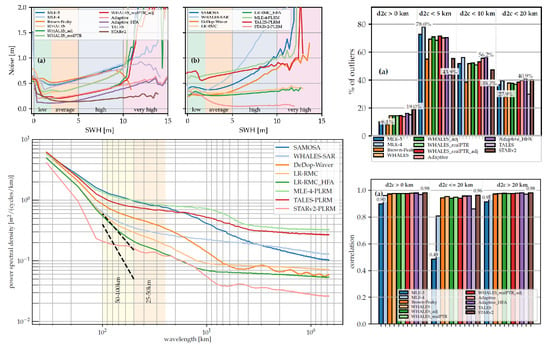
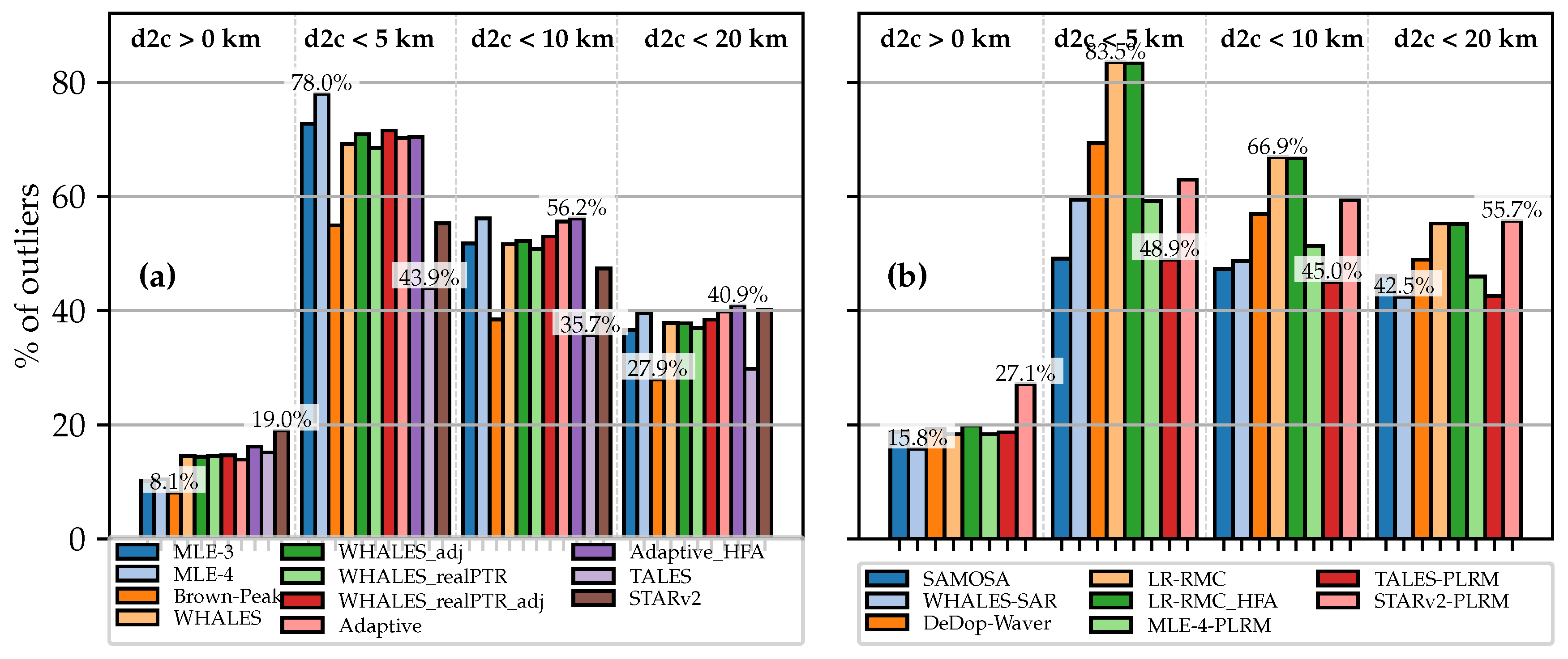
Figure 3 shows the number of total outliers of J3 vs. S3A in dependence of the dist2coast. For open-ocean scenarios, Brown-Peaky (J3) and WHALES-SAR (S3A) have the least amount of total outliers, accounting for 8.1% and 15.8%. The outliers of all retrackers stay below 20%, with the exception of STARv2-PLRM, which amounts to 27%. The J3 retrackers tend to be less prone to outliers, but since the two satellites follow different ground tracks, this hypothesis needs to be considered with care. Among the new retrackers, J3 datasets contain less outliers. This is likely to be a consequence of a more conservative use of the quality flag, since in the standard products (MLE-3 for J3 and SAMOSA for S3A) the opposite is observed.

When approaching the coast, the number of outliers is significantly increased for both LRM and DDA retrackers. The number of outliers range from ∼28% to ∼55% (LRM) and from ∼43% to ∼60% (DDA) for the best performing retrackers (approaching coast in the intervals 20, 10, and 5 km), which are Brown-Peaky and TALES for J3 and SAMOSA, WHALES-SAR, and TALES-PLRM for S3A. It appears that the number of outliers quasi-linearly increase with a decreasing dist2coast. The differences of the amount of total outliers can be quite large, for example, when considering areas that are very close to the coast (less than 5 km), SAMOSA is able to produce estimates for almost 50% of the measurements, whereas Adaptive retrieves only 16.5% of valid SWH samples.

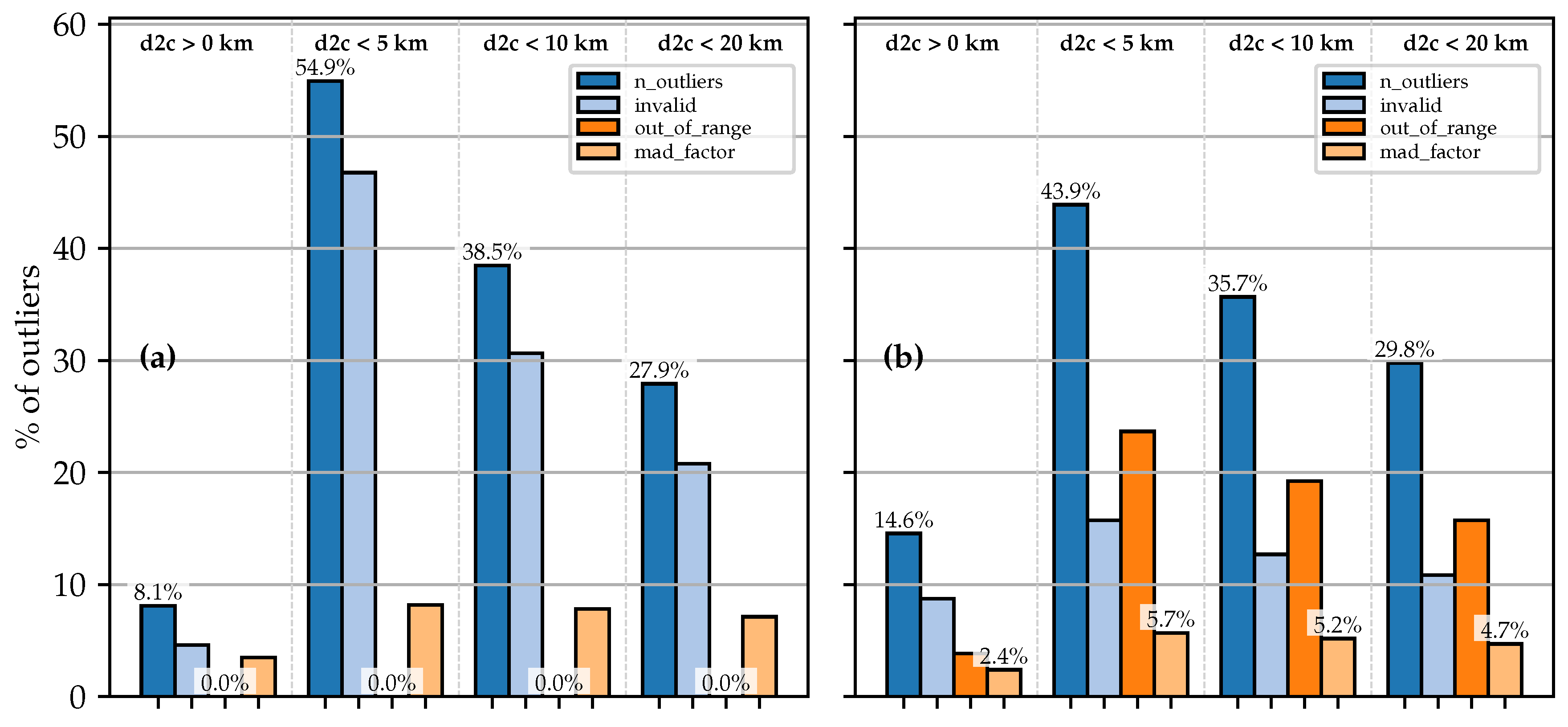
Figure 4 depicts the distribution of the outliers types invalid, out_of_range, and mad_factor as a function of dist2coast for the retrackers Brown-Peaky and TALES. They both follow a subwaveform approach that discards the trailing edge of the waveform, which is mostly contaminated by spurious signals in the coastal zone. One might, thus, expect a similar outlier behaviour, but their number of outliers differ. TALES exhibits a significant amount of about 15–23% of out_of_range outliers, whereas Brown-Peaky shows none but instead an increased amount of invalid estimates (21% vs. 11% for dist2coast < 20 km). This underlines the role of quality flag: It is up to the strategy of the individual retracker, whether to decide if an estimate is set to be bad or remained as a potential outlier (out_of_range or mad_factor). Interestingly, in general, the fraction of mad_factor outliers is increased only slightly by a factor of about two when approaching coast, whereas the total amount of outliers increases significantly, meaning that the mad_factor does only weakly depend upon the dist2coast. In contrast, the estimate is either good or very bad or missing in the coastal zone, yielding the measurement to be an outlier of type invalid or out_of_range.

In Figure 5, the outlier types of the two DDA retrackers SAMOSA and WHALES-SAR are shown. Both exhibit a low amount of total outliers, as shown in Figure 3. SAMOSA’s major fraction of outliers mostly accounts for invalid estimates, no out_of_range values, and only few mad_factor-type outliers. This signifies that it is capable of correctly identifying which values might be reliable estimates. The total amount remains relatively constant in the coastal zone with about 48%, even when further decreasing the dist2coast. In comparison, as shown in Figure 5b, WHALES-SAR (which still exhibits one of the best outlier characteristics of the investigated retrackers) sets some SWH estimates to out_of_range values. This might arise from the fact that only a subwaveform is considered. Likewise, as with SAMOSA, the number of invalid points make up the majority of outliers and the number of mad_factor samples remain relatively constant between about 3–5%.

To conclude the outlier analysis, one can state the following points:

• The number of outliers is significantly increased in the coastal zone and increases further when approaching coast.
• In open-ocean, the number of total outliers amounts to less than 20%.
• Most of the retrackers’ outlier types are invalid samples, which originate from measurements, the quality flag of which is poorly defined.

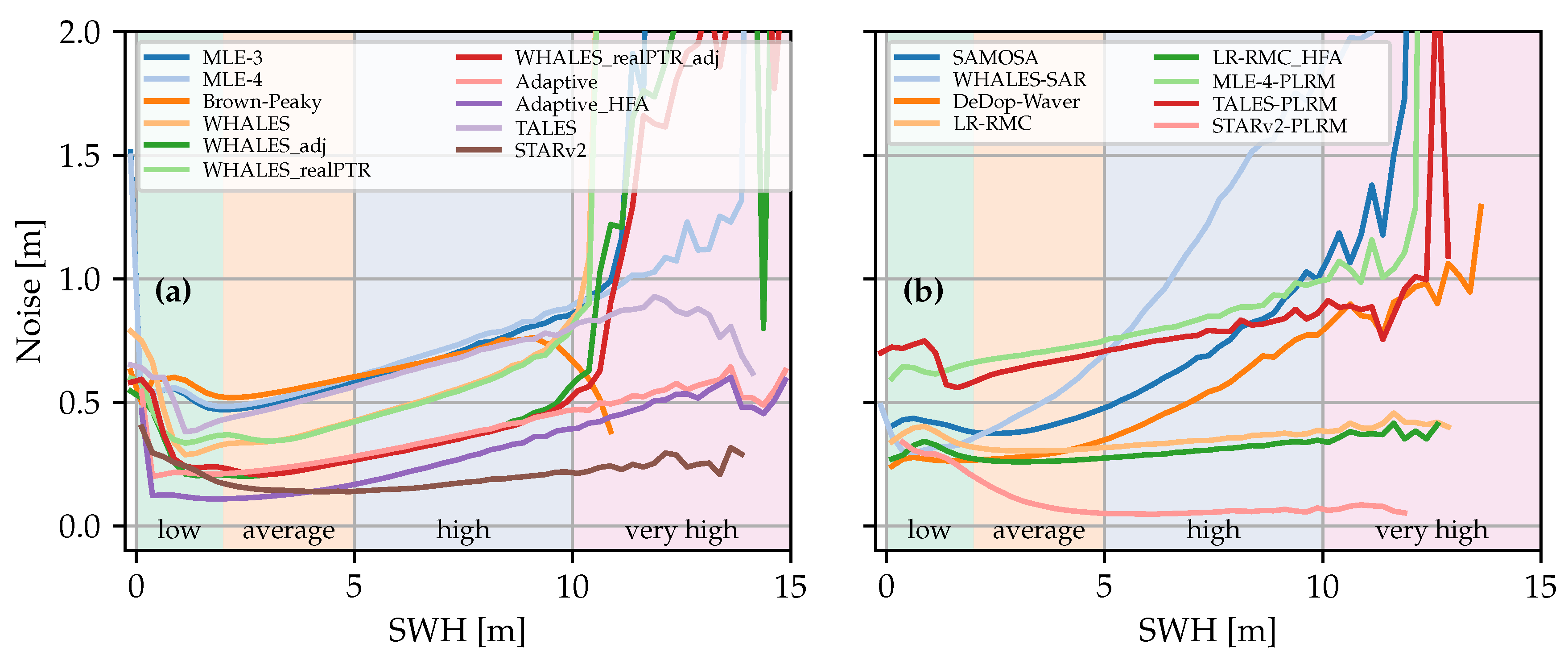
4.2. Noise Analysis

In this section, the intrinsic noise of the retracked datasets is evaluated. As described in Section 3.3, the noise is defined as the SD of a 20-Hz measurement of the along-track series.

As already noted in Section 2, an important fact to consider is that some of the investigated retracked datasets already have a denoising technique applied:

• J3: WHALES_adj, WHALES_realPTR_adj, Adaptive_HFA, and STARv2
• S3A: LR-RMC_HFA, STARv2-PLRM

These datasets exhibit a reduced noise performance and need to be evaluated separately. It also has to be noted that some of the denoising techniques can be applied independently a-posteriori after the SWH estimates (L2 data) were retrieved so they can be applied to arbitrary retrackers. Other retrackers, such as the STARv2/STARv2-PLRM algorithm, have an inherent denoising implied.

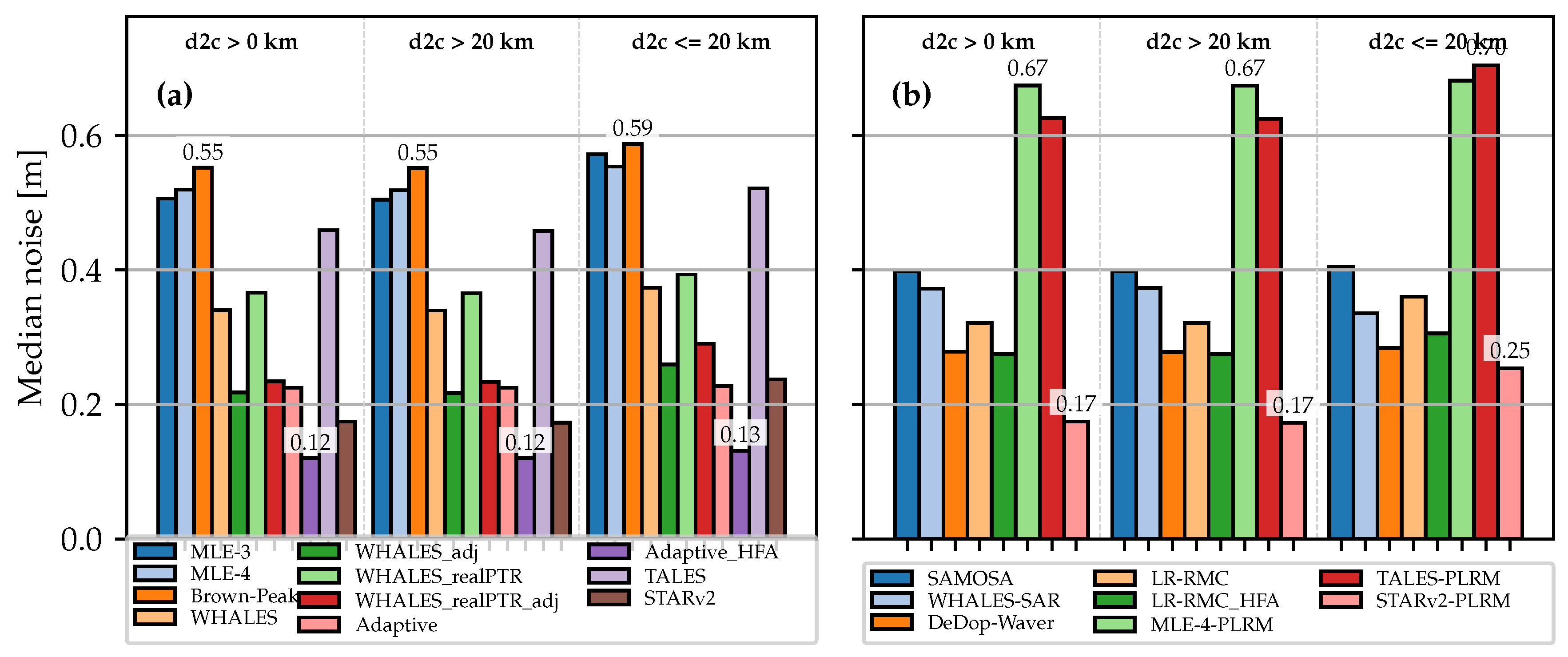
Figure 6 depicts the median noise values of (a) J3 and (b) S3A in dependence of the area of interest: overall, coast, and open-ocean. For the J3/LRM-retrackers without denoising, Adaptive and WHALES have the least and second least median noise values of about 0.23 m. While also including denoised datasets into consideration, Adaptive_HFA has the lowest median noise values with about 0.12 m, followed by STARv2 with about 0.18 m. For the S3A algorithms without denoising, DeDop-Waver shows the lowest median noise values with about 0.32 m. Among the denoised algorithms, STARv2-PLRM has the least median noise values with a slight increase for the coastal scenario from 0.17 to 0.25 m. This demonstrates the effectiveness of the used denoising techniques.

When analysing the dependence of the median noise values for open-ocean and coastal scenarios, one can notice a slight increase of noise, which is more or less pronounced on the individual algorithms. For instance, STARv2’s value is increased from about 0.18 to about 0.24 m, whereas Adaptive_HFA’s value is increased by just 0.01 m. In conclusion, it can be stated that there is only a minor dependence on the dist2coast.

Figure 7 depicts the noise as a function of SWH and the different sea states, as defined in Table 4. The plots demonstrate the strong dependence of the sea state. The results are in accordance with the ones shown in Figure 6.

For LRM, Adaptive exhibits the best noise performance for all sea states (no denoising applied). With denoising applied, Adaptive_HFA has the lowest noise level for low and average sea states, whereas STARv2 outperforms Adaptive_HFA for high and very high conditions.

With respect to S3A and low sea states, the noise levels of WHALES-SAR, DeDop-Waver, LR-RMC_HFA (denoised), and STARv2 (denoised) are at a similar level. For average, high and very high sea states, STARv2-PLRM shows significantly low noise values. This might be explained by the nature of the STARv2-PLRM algorithm, for which neighbouring SWH estimates are taken into account for reducing abrupt changes in the estimates and thus reducing the SD of the 20-Hz measurements (the same applies to the LRM version of STARv2). Thereafter comes the LR-RMC algorithm as the second best of the S3A retrackers at average, high, and very high sea states.

For very low significant wave heights (SWHs) of less than 1 m, one can observe an increased noise level. This is due to the fact that sea states with very low wave heights induce a waveform with a very steep slope of the leading edge, which thus is undersampled. Smith and Scharroo [16] have investigated this issue and suggested a simple zero-padding, with which this effect can be mitigated.

Comparing the noise level of the standard retrackers MLE-4 and SAMOSA (LRM vs. DDA) for low and average sea states, one can conclude that the performance is improved significantly, which is in accordance with the literature [59].

Furthermore, it can be stated that most of the novel retrackers show significant improvements across all sea states, as compared with the standard retrackers MLE-4 and SAMOSA. This is particularly pronounced for high and very high sea states, for which both retrackers show at least twice as much noise level as compared to the novel approaches.

When comparing the absolute noise levels evaluated here with those mentioned in the literature, one can observe that they differ from each other. For instance, [27] has conducted a study in the German Bight and estimated the noise values of 6.7 and 13 cm (for SWH values around 2 m) for DDA and PLRM (considering open-ocean measurements with dist2coast>=10 km), respectively. In [60], noise values were retrieved to be 8.5 cm and 11.09 for DDA and LRM for open-ocean scenarios across all sea states. [15] has compared the noise for a full cycle of the missions J3, S3B-LRM, and S3B-SARM, and estimated them to be 0.50 cm, 0.47 cm, and 0.38 m for SWH values of around 2 m, respectively. From this, it can be concluded, that the intrinsic noise performance strongly depends upon the region of interest, the sea state, and whether the coastal zone is included or not in the considerations. With the values evaluated in this RR exercise, ranging from 0.12 to 0.70 m, the findings are in accordance to the literature.

To sum up the noise analysis, the following can be stated:

• The intrinsic noise shows only a minor dependence on the dist2coast and strong dependence on the sea state.
• The noise of most of the novel retracking algorithms considered is lower than the baseline.
• DDA retrackers show a better noise performance than their adapted PLRM counterpart.

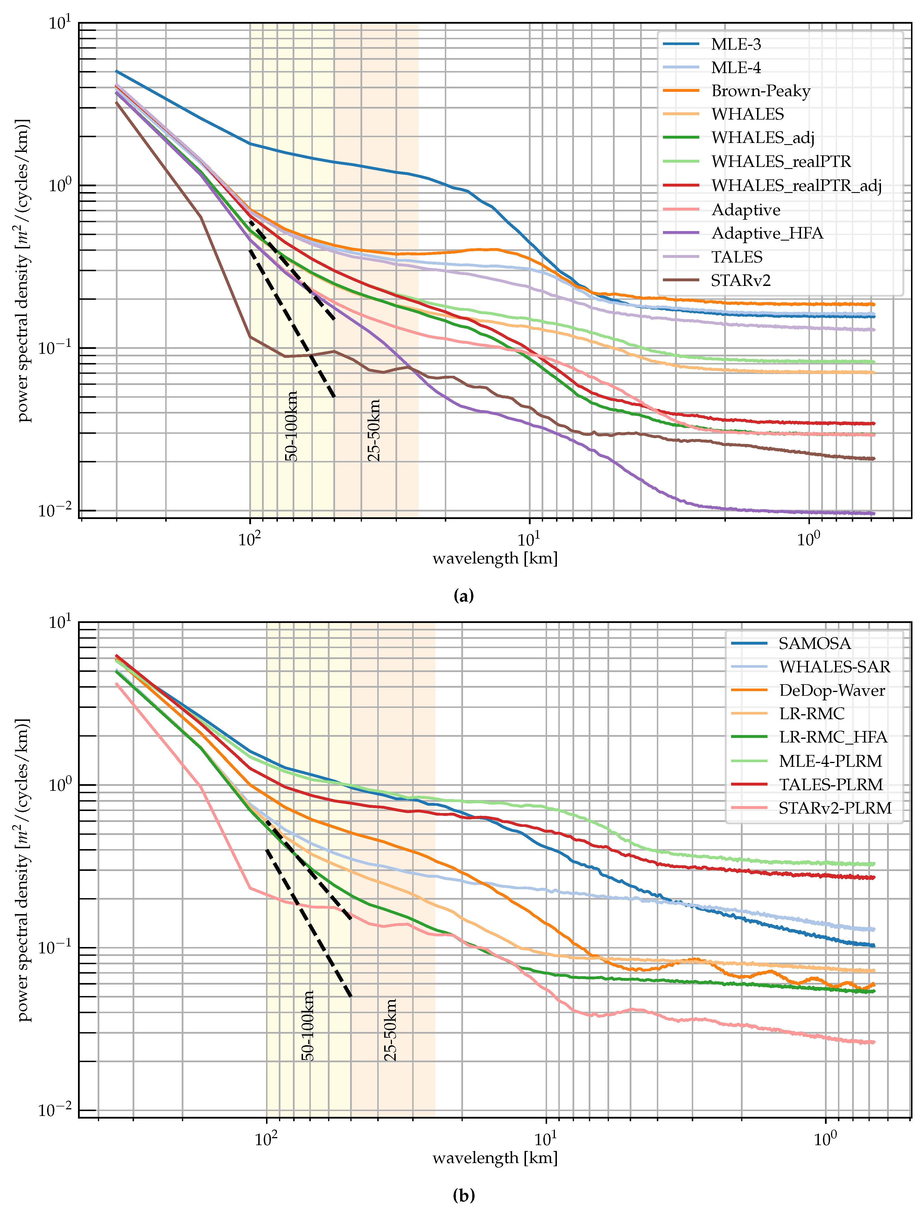
4.3. Wave Spectral Variability Analysis

4.3.1. Jason-3

Spectra of J3 LRM data were determined for around 62,000 segments (each including 1024 20-Hz measurements), except for TALES for which there were only ∼50,000 segments because of the greater occurrence of flagged data for that retracker. The spectra of S3A data were estimated for about 24,000 segments for most of the retrackers. For TALES, only 15,000 segments were available. At long wavelengths, the spectra for all retrackers should predominantly relate to the real geophysical signal, whilst at the smallest wavelengths, it is similar to the measure of sensitivity to fading noise shown in Figure 6. In between these wavelengths, there are a variety of different behaviours.

First, considering the J3 LRM data (Figure 8a), one notes that the de facto reference provided by MLE-4 exhibits a “spectral hump” between 8 and 50 km [14]. Most of the newer algorithms have lower spectra levels than that within this band, whereas the simpler algorithm MLE-3 has higher noise levels for wavelengths of 8 km and upwards. This may indicate that the actual waveform shapes are responding to other factors, for example, slight variations in sea surface skewness [61] or in the angle between the surface perpendicular and the antenna boresight that are better represented by the MLE-4 algorithm. In the absence of any waveform bins being deemed to contain anomalous peaks, the Brown-Peaky algorithm effectively reverts to MLE-4; thus, its mean/median spectrum is similar to that of MLE-4, although it does exhibit extra variability in the 8-25 km band. TALES shows slightly lower noise levels than MLE-4 for all scales below 25 km, but the difference is always less than 10%.

The four flavours of WHALES have almost identical behaviour at large wavelengths, with their associated power levels below 50 km being at least 45% lower than for MLE-4, with those having a correction for covariant errors [35] being significantly lower again for scales under 15 km. Those versions of WHALES incorporating a bespoke PTR correction show slightly greater noise levels than those corrected using an empirical LUT. For the Adaptive algorithm, which already has one of the lowest noise levels, the version with the HFA again reduces the noise level at scales below ∼50 km. This latter adjustment is effective over a longer span of scales (i.e., all those below 50 km) than the WHALES version (<15 km) partially because it calculates height anomalies relative to a longer along-track scale.

Finally, the performance of STARv2 is noteworthy, in that it achieves the lowest spectral levels in the 25–100 km range of wavelengths but has produced an unexpected spectral shape. The procedure it uses for fitting a SWH profile through the cloud of solution space certainly amounts to significant filtering, reducing the noise levels; however, the cause of the undulations in the spectrum are not yet understood.

Whilst there are many buoys providing frequency and directional spectra of waves, these give no indication on the spatial variability of wave properties. For spatial scales of the order 10 to 200 km and away from shorelines, the variability of SWH seems to be dominated by the effect of surface current on the waves, with a spectrum of SWH that closely follows the shape of the spectrum of the current kinetic energy [62]. The negative slope of the kinetic energy (KE) spectrum reflects the cascade of energy from large mesoscale features to smaller scales, with a typical slope close to $k^{-2}$ [63,64]. The influence of wave–current interactions means that different wave spectra may be encountered in regions with pronounced current variability [Villas-Boas et al., in prep.]. The dashed lines indicate slopes in the 50–100 km range of $k^{-2}$ and $k^{-3}$, as aids for comparison as been done in [37].

4.3.2. Sentinel-3A

Figure 8b shows the spectra obtained from the S3A data. At the long wavelength end (∼300 km), most curves converge to the same value as noted for J3 because, at this scale, the variability in SWH is dominated by the real large-scale signal. Again, TALES has slightly lower power levels than MLE-4 through all scales, with less of a pronounced spectral hump around 10 km, and the STARv2 retracker produces much lower levels but does not have the features manifest in the output of other algorithms. At scales below 100 km, the algorithms based on PLRM data broadly match their equivalents for J3; however, the noise levels are higher because these waveforms correspond to the averaging of ∼36 independent pulses, whereas for J3 it is 90. The SWH spectra for MLE-4-PLRM and TALES-PLRM at scales below ∼30 km are roughly twice that of their J3 analogues; for STARv2-PLRM, the factor is only ∼1.4, but this may be due to the details of the process used to fit an SWH profile through its solution space.

Of the retrackers that make use of the DDA waveforms, all the new ones show reduced noise levels compared with SAMOSA. The WHALES-SAR algorithm shows much lower spectral levels than SAMOSA between 4 and 200 km, with SAMOSA only outperforming it at the finest scales. The LR-RMC algorithm has significantly lower noise levels than WHALES or SAMOSA over all scales below ∼50 km, with the application of the HFA significantly reducing noise levels at wavelengths below 50 km. The DDA retracker DeDop-Waver also has very low noise levels at the shortest scales but shows undulations in the spectrum below 7 km.

The DeDop-Waver dataset was originally calculated on a different set of nominal waveform locations, and then linearly interpolated to the same locations as the other datasets. Simulation work by Chris Ray (pers. comm. 2020) suggests that this is likely to be the cause of the undulations in its spectra. This linear interpolation will also cause the analysis of its noise levels to lead to slightly lower values than would have been the case if that dataset had matched the same locations as the others.

There have been many authors in the last decade who have looked at spectra of sea surface height from altimetry, with the largest wavelengths showing a clear geophysical signal, the smallest wavelengths being totally measurement noise, and with indications of a “spectral hump” [14] in the range of 8 to 50 km. Sandwell and Smith [40] had earlier shown a plateau in the spectrum associated with MLE-3 applied to ERS-1 data, but as their “two-pass” retracking solution involved filtering the initial SWH estimates, it does not yield a meaningful curve for SWH spectra. The most useful prior example is from the seminal work by Dibarboure et al. [14] as they contrast SWH spectra from Jason-2 (J2), CS2 DDA and CS2 PLRM, noting that the much smaller along-track resolution of the DDA led to spectra without the hump observed in other datasets. That paper showed major gains from DDA processing but was based only on sections across a patch of quiescent ocean. Our analysis, averaging spectra throughout the global ocean still shows “power excess” in the 10 to 50 km band, but this may reflect different pertinent geophysical processes in this regime, such as wave-current interactions.

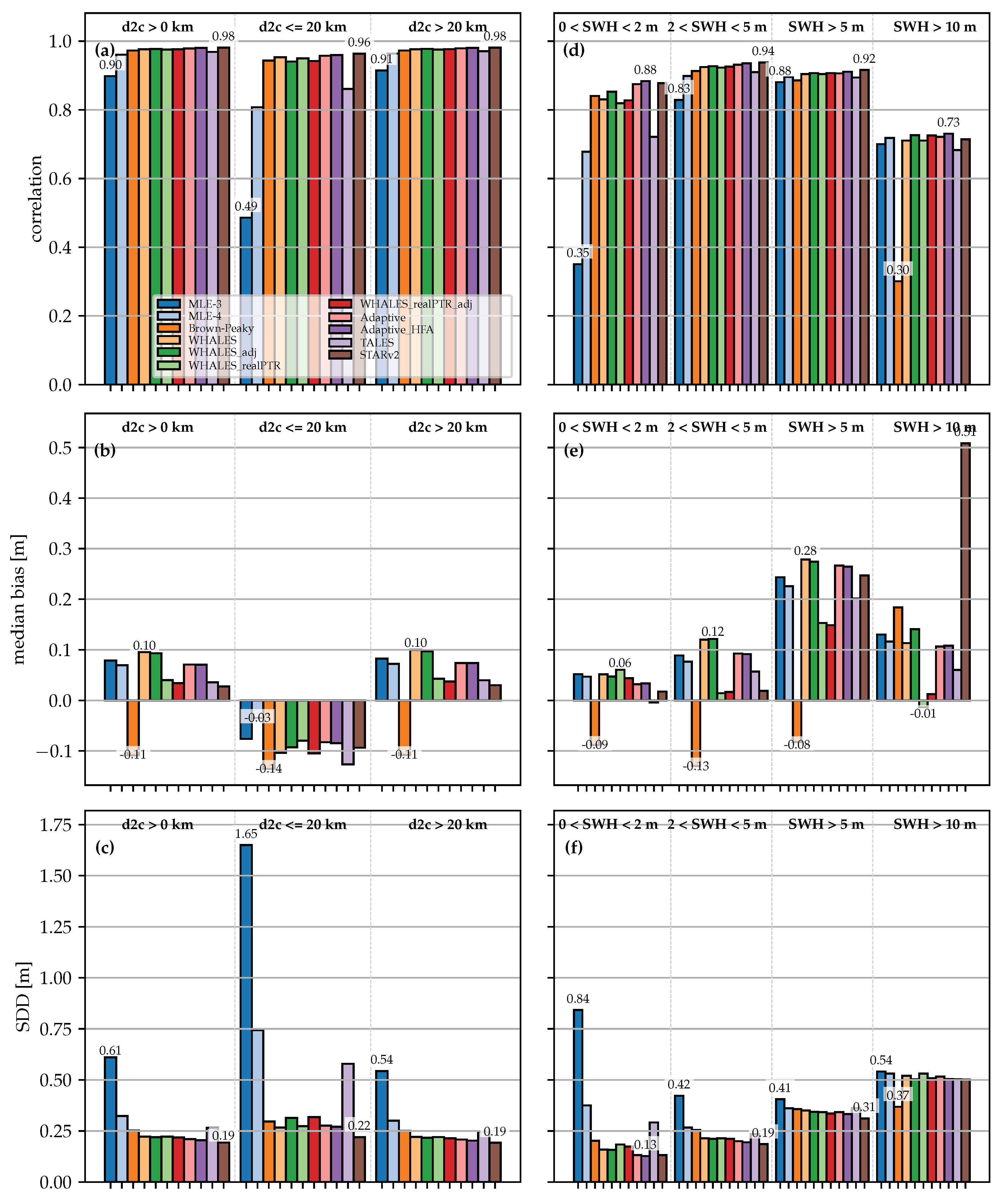
4.4. Comparison against Wave Model

The statistics of the comparison of the 1-Hz retracked data against the ERA5-based hindcast (ERA5-h) wave model, which does not assimilate any satellite altimetry data, are shown in Figure 9 and Figure 10 for J3 and S3A as a function of dist2coast and the sea state on the left and right columns, respectively. As described in Section 3, the three metrics correlation, median bias, and SDD are presented and discussed in this section.

It needs to be emphasised at this point of the analysis that the comparison against the wave model is limited to the resolution of the ERA5-h wave model (which is 18 km). Since the posting rate of the SWH series and the model are reduced to 1-Hz, potential high-frequency variations of the SWH series might, thus, be masked or some retrackers that inherently smoothen the SWH series might benefit from this type of analysis (e.g., STARv2 or the _HFA variants). In consequence, this means that if a retracking algorithm, such as STARv2, is strongly filtering an SWH series, it might show an excellent correlation against the wave model and a low SDD, which is shown in the following subsections. However, at the same time, the smoothened SWH series lacks a significant amount of energy, as discussed in Section 4.3.

Moreover, a wave model has limitations in the coastal zone, where wave interactions with bathymetry and land-shading effects often require regional nested very high resolution models to improve the simulations. Therefore, this assessment is complementary to the use of a ground-truth such as a large buoy dataset but can still be useful to derive further noise characteristics of the retracking w.r.t. an independent source and erroneous estimates of SWH (although realistic and therefore not detectable by the outlier analysis) near the coast.

4.4.1. Jason-3

Figure 9 depicts the comparison statistics against the ERA5-h model for the retracked Jason-3 (J3) datasets. In the first row, the correlation coefficient is presented as a function of dist2coast and sea state. Apart from MLE-3, all retrackers show a very good correlation with a coefficient of around 0.97 for the overall and open-ocean scenario. However, in the coastal zone, MLE-3, MLE-4, and TALES show a deteriorated performance with a correlation of 0.8–0.85 (0.49 for MLE-3). The rest of the retrackers show a very high correlation of 0.96 in the coastal zone. For average and high sea state the differences are less pronounced with most of the retrackers showing a high correlation of around 0.92. For low sea states, Adaptive, and STARv2 prove the best correlation with values of around 0.87, whereas MLE-3, MLE-4, and TALES show degraded correlations. For very high sea states, all retrackers (apart from Brown-Peaky) show similar degraded correlations of around 0.72.

The median bias in the second row of Figure 9 depicts how much the SWH is different from the model, with lower values indicating a more accurate dataset. In this case, the median bias depends on both the area of interest and the sea state. For coastal scenarios, it can be said that the estimates tend to be overestimated (meaning the retracked value is higher than the model, recall Equation (2)), whereas for open-ocean the retrieval are rather underestimated. With an increasing sea state, the median bias also tends to increase. STARv2 strongly underestimates large wave heights, showing a median bias of 0.51 m. (Figure 7-top [23]) has plotted the monthly bias for MLE-4 (J2 mission), which ranges at around 0.1 m (sign was aligned, since the definition of the bias is vice versa), which is in accordance of the median bias value of around 0.08 m in Figure 9 (centre row, left for dist2coast > 0 km).

The last row of Figure 9 depicts the SDD. All retrackers show comparable SDD values of around 0.20–0.40 m for most of the conditions with the exception of increased values for very high sea states. MLE-3, MLE-4, and (partially) TALES show increased values for low and average sea states and particularly in the coastal zone. In [22], an SDD value of 0.20 m was reported for MLE-4 for the SARAL/AltiKa mission, which is in good agreement with the value of about 0.25 m, when considering an average sea state as shown in Figure 9 (last row, right).

In conclusion, most of the retrackers show similar performances in terms of correlation, median bias, and SDD for coastal, open-ocean scenarios and most of the sea states, when comparing the 1-Hz retracked data with the ERA5-h wave model. MLE-3, MLE-4, and TALES exhibit a deteriorated performance, especially in the coastal zone.

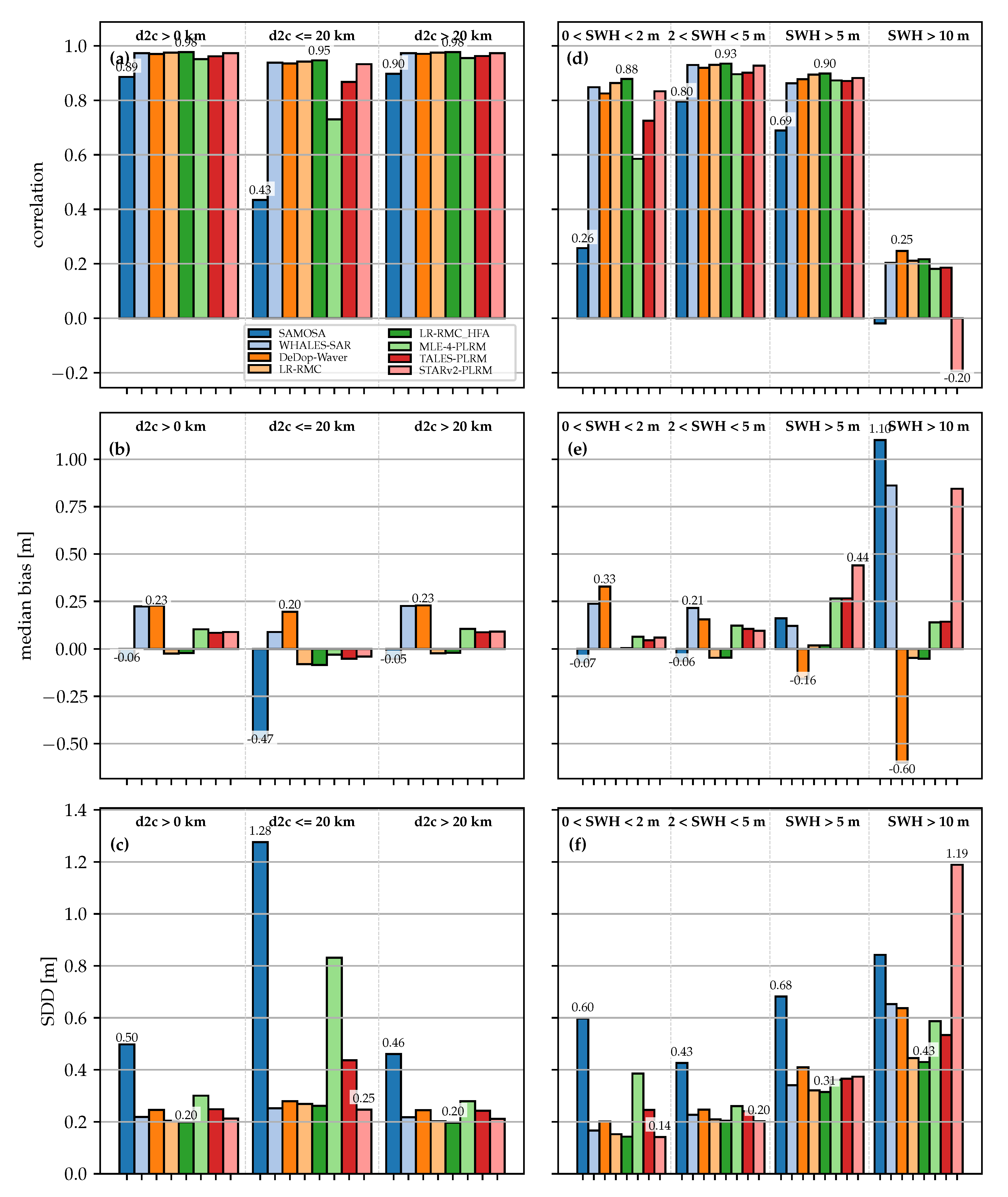
4.4.2. Sentinel-3A

The assessed Sentinel-3A (S3A) retrackers show for the overall and open-ocean scenarios a very high correlation against the ERA5-h wave model of around 0.96 (with the exception of SAMOSA: 0.89). This also applies to the coastal zone, where all retrackers exhibit a high correlation of around 0.95, with the exception of MLE-4-PLRM (~0.75), TALES-PLRM (~0.85) and the standard L2 product SAMOSA (0.43). All retrackers (apart of SAMOSA) show a very good correlation of ~0.9 of for average and high sea states. With respect to low sea states, LR-RMC/LR-RMC_HFA have the highest correlation of 0.88, followed by WHALES-SAR, STARv2-PLRM, and DeDop-Waver, which amount to around 0.83. SAMOSA shows the worst correlation across all sea states. None of the algorithms are able to correctly retrieve very high sea states, with an average correlation of about 0.2 (SAMOSA: around 0.0). The inaccurate estimates for very high sea states might be explained by the very few samples that are available in all datasets: Out of the 512 netCDF files (pole-to-pole tracks), there are only around 260 1-Hz SWH estimates apparent (in comparison for the J3 analysis: around 2100). STARv2-PLRM shows an inverse correlation of −0.20 for very high sea states, which again can be attributed to the scales of denoising that are likely to be too wide to correctly observe areas with very high waves. The authors of [23] have reported correlation values of 0.98 and 0.94 for the CS2 NE Atlantic and Pacific Box, with the latter one being placed in the open-ocean. These are in a rough accordance to the evaluated value of 0.90, as shown in Figure 10 (top row, left, dist2coast > 0 km).

The median bias has only a minor dependence of the dist2coast. LR-RMC, LR-RMC_HFA, MLE-4-PLRM, TALES-PLRM, and STARv2-PLRM show a very small median bias of less than 0.10 m in the coastal zone. SAMOSA exhibits a very large bias in the coastal zone with a value of −0.47 m, which is in accordance to the degraded correlation, as discussed before. The LR-RMC variants incorporate almost no median bias in open-ocean and in all sea states with less than 0.05 m. For very high sea states, most of the retrackers have a high median bias. This is as expected from the correlation analysis and might be due to the very few samples that are available for such high sea states. The bias that was retrieved for SAMOSA in the NE Atlantic or Pacific Box of CS2 is very low with values of about −0.08 m and −0.03 m (sign swapped by authors, since the definition of the bias is swapped), as shown in (Figure 5 [23]), which is very well in accordance with the bias value of −0.06 m for the average sea state (Figure 10, centre row, right).

As the majority of the retrackers (WHALES-SAR, DeDop-Waver, LR-RMC/LR-RMC_HFA and STARv2-PLRM) shows a good very good correlation in the coastal zone, the SDD also amounts to a very low value of around 0.25 m. All LR-RMC ranks best among the non-denoised algorithms with a strongly deteriorated performance in the coastal zone, showing an SDD value of 0.65 m. Most of the retrackers show an increasing SDD for the average, high, and very high sea states starting from around 0.30 m. Particularly the PLRM variants (excluding STARv2-PLRM because of its inherent denoising) show increased SDDs both in the coastal zone and for low and very high sea states. This is in agreement with the findings of (Figure 21 [28]), which demonstrates a significantly increased SD for TALES as compared to an improved SAMOSA-based DDA retracker (SAMOSA+) within the coastal zone. The authors of [23] have assessed SDD values of 0.30 and 0.18 m for the CS2 NE Atlantic Box and Pacific Box. Compared with the value of 0.50 m of SAMOSA as shown in Figure 10 (bottom row, left), the difference is quite significant but might be explained with smoother and less variable conditions in the tropical Pacifics (in the dataset of [23]). Another reason might be the extreme sea states that are included in our investigated datasets, which show a poor correlation as elaborated before.

To sum up the results of the comparison against the ERA5-h analysis, the retrackers WHALES-SAR, DeDop-Waver, LR-RMC, and STARv2-PLRM show all a comparable good accuracy and precision. The differences are only minor for both open-ocean and coastal scenarios. LR-RMC shows the smallest median bias values for open-ocean and across all sea states. The differences in terms of correlation and SDD are not significant for the retrackers WHALES-SAR, DeDop-Waver, LR-RMC, and STARv2-PLRM. In general, the estimates for very high sea states are very poor for all retrackers, very likely due to the scarcity of available records.

An important fact that was not considered in this evaluation is the numbers of valid 1-Hz measurements that is mainly attributed to the supplied quality flag. As described in Section 4.1, the retrackers show significant differences in terms of number of outliers. Two of the best performing algorithms LR-RMC and STARv2-PLRM also show the highest number of outliers in the coastal zone with less than 20 km. It becomes obvious here that it is a trade-off between quality and quantity of the measuerements.

4.5. Comparison against In-Situ Data

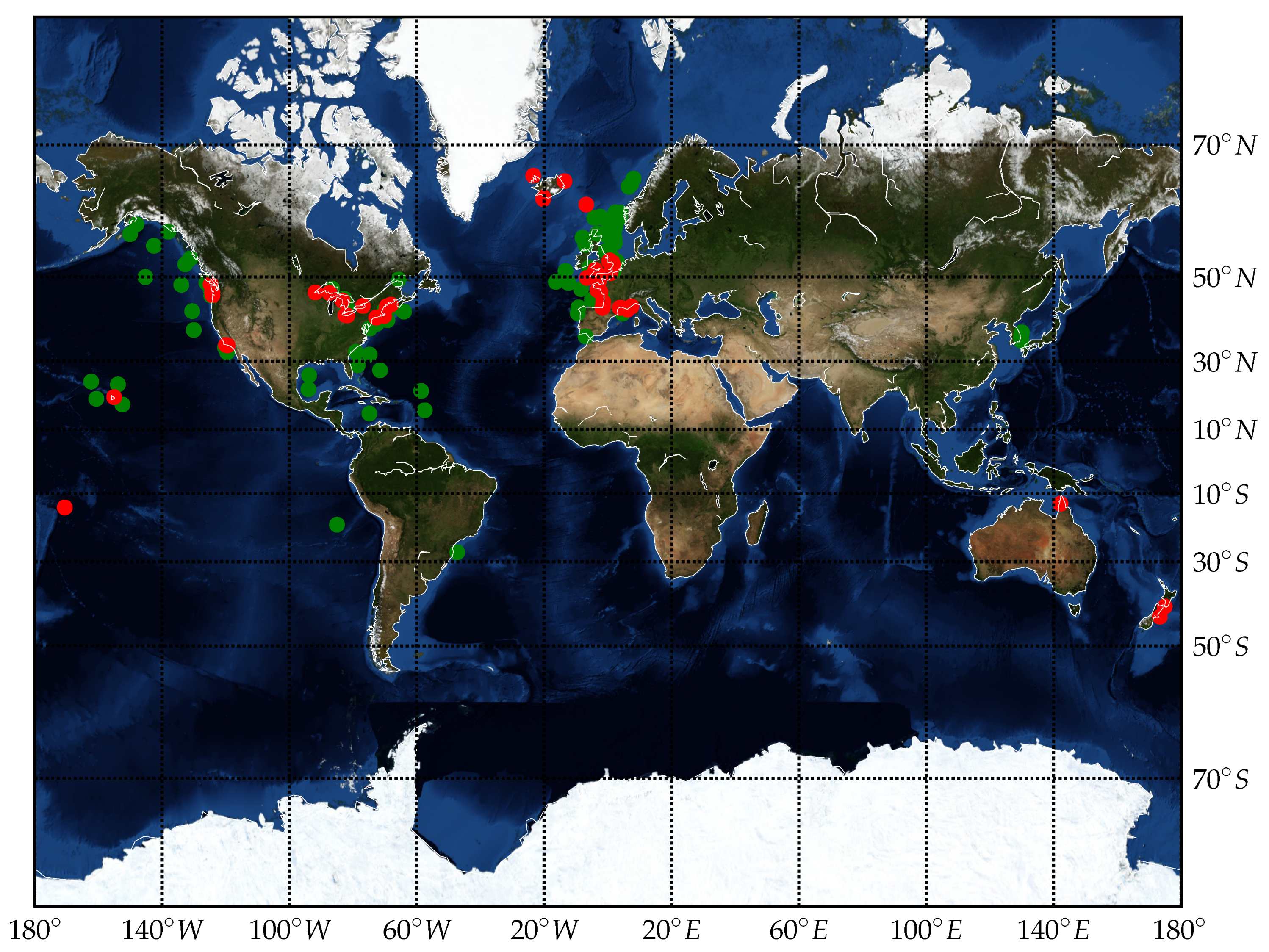
The performance of retracking algorithms is estimated by using buoy datasets described in Section 2. The J3 dataset contains about 7100 records of SWH collocated with altimeter individual tracks and S3A dataset contains about 2500 collocated records. These data are processed and compared with the outputs of different retracking algorithms, as described in Section 3.6. The results of this comparison are summarised in Figure 11 for J3 and Figure 12 for S3. The statistical metrics are estimated as a function of dist2coast for all available data, open-ocean, and coastal zone and also of sea states. It is worth noting here that comparison results are not available for sea state SWH > 10 m, since the in-situ buoy dataset only contains records with smaller waves heights.

To identify unreliable buoy measurements, an error ${\mathrm{Err}}_{buoy}$ is estimated between each buoy and retracked data (see Section 3.6). In total, 4 out of 125 buoys in J3 dataset and 1 out of 170 buoys in S3A dataset were identified as completely unreliable and discarded from the comparison with altimeter measurements.

4.5.1. Jason-3

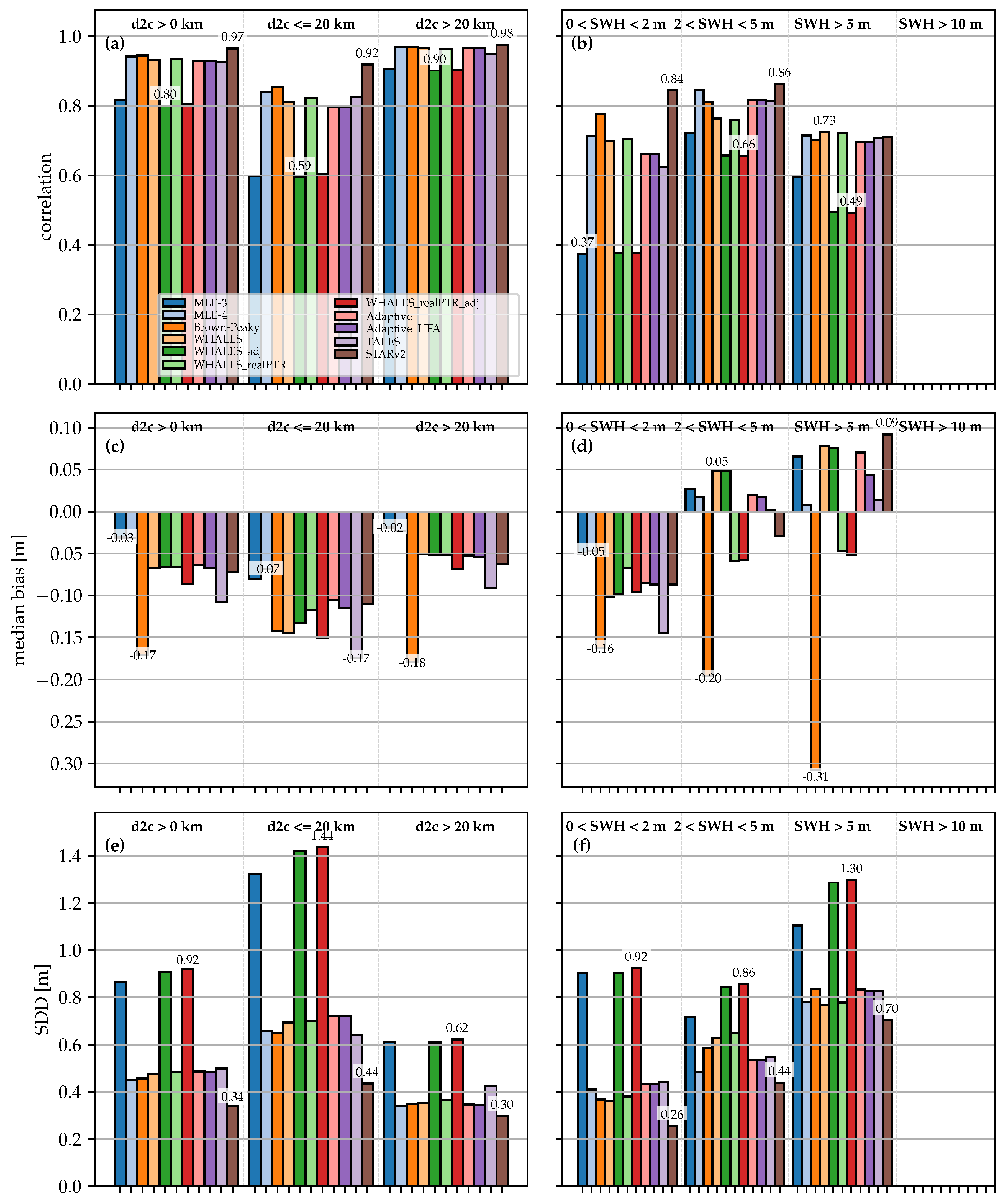
The estimates of correlation coefficients for coastal waters, open-ocean, and different sea state conditions, are shown in the top row of Figure 11. Overall, the highest correlation is found for the STARv2 retracking algorithm and the lowest correlation is noted for MLE-3, WHALES_adj and WHALES_realPTR_adj. At the same time, MLE-4, WHALES and WHALES_realPTR retrackers demonstrate a performance similar to that for Adaptive and TALES retrackers. It is seen in the left plot in Figure 11 that, for all retrackers, the dist2coast has a significant effect on their performance. For STARv2 retracker, the correlation coefficient reduces from 0.98 in the open-ocean to 0.92 in the coastal zone, and for WHALES_adj it drops from 0.9 to 0.59. The right top plot in Figure 11 shows how the performance of retracking algorithms is affected by the sea state condition. For all retrackers, the best performance is achieved for average sea states, while for low sea states are the most challenging one. For all three sea states in the plot, the best performance is demonstrated by STARv2 retracker and the second best is Brown-Peaky. The worst results are given by MLE-3, WHALES_adj and WHALES_realPTR_adj retrackers.

The middle row in Figure 11 shows median bias (i.e., buoy minus altimeter) for different conditions, such as dist2coast and sea states. In these plots, MLE-3 and MLE-4 retrackers produce the lowest bias values. Brown-Peaky retracker has the highest bias with the exception of the coastal zone where the highest value belongs to TALES algorithm. For low sea states, the median bias is negative for all of the tested retracker algorithms; this reflects that for SWH < 1 m, the waveform bins at ∼0.47 m separation, are unable to resolve well the slope of the leading edge, and thus all algorithms tend to give values that are too large. For high sea states (SWH > 5 m), the median bias remains negative only for Brown-Peaky, WHALES_realPTR and WHALES_realPTR_adj retrackers. Hence, limitations of retracker algorithms become more apparent in calm sea conditions.

Overall, the median bias values are much smaller than SDD values shown in the plots in the bottom row of Figure 11. For the open-ocean and coastal zone, the SDD metric behaves similar to the correlation coefficient. The best results are achieved by STARv2 retracker and the worst performance is demonstrated by MLE-3, WHALES-adj and WHALES_realPTR_adj. These three algorithms show the worst results for the average sea state conditions and their performance is also poor for the low and high sea states. STARv2 has the lowest values in all three regimes and gives its best performance in terms of SDD for the low sea states and the worst one for the rough sea. Generally, other retrackers demonstrate similar behaviour, with increased SDD at higher SWH.

4.5.2. Sentinel-3A

Figure 12 shows the comparison results with buoy data for five DDA retracker algorithms and three PLRM algorithms. The plots of correlation coefficient show the worst performance is achieved by SAMOSA retracker and MLE-4-PLRM is the second worst. All other retrackers demonstrate similar values of correlation coefficient. In general, the correlation is higher for the open-ocean than for the coastal zone. For the average sea state, it is slightly higher than for the low sea state, but values are significantly decreased for high sea states. However, the plots do not show any obvious advantages of DDA over PLRM retracking algorithms.

In contrast to similar plots for J3, the plots of SWH median bias Figure 12 shows a changing sign of offset for different retrackers. For the coastal zone and for rough sea conditions, the highest and negative bias is estimated for the SAMOSA retracker. The lowest bias is found for the MLE-4-PLRM algorithm in the open-ocean and for the average sea state.

The plots of SDD in Figure 12 confirm the poor performance of SAMOSA retracker in all conditions and sea states, revealed by the correlation coefficient. While MLE-4-PLRM is the second worst retracker in the plots after SAMOSA, it demonstrates relatively good accuracy in the open-ocean and for the high sea state conditions. For all other retrackers, the SDD values are getting higher in the coastal zone and for average or high sea states. The plots of SDD metric show STARv2 and LR-RMC (and LR-RMC_HFA) giving the best results but do not reveal any advantages of PLRM over DDA retrackers or vice versa.

There are dangers in comparing our results with prior studies, as the period of study, the mean wave conditions, and the quality of the buoy dataset may all vary. This is why a full comparative evaluation of algorithms should always be performed applying the algorithms to the same altimeter data and with the same in-situ measurements. Our work showed a typical mismatch, SDD, in the open-ocean of 0.35 m for J3 and 0.30 m for S3, with this value encompassing buoy measurement error, altimeter error, and spatiotemporal variations between the buoy and altimeter locations and times of recording. These SDD values increased to 0.8 and 0.4 m, respectively, when the buoy SWH exceeds 5 m. For typical open-ocean conditions, Yang and Zhang [25] had SDD values of 0.25 m and 0.30 m for S3 DDA and PLRM estimates, respectively, whilst earlier analyses for other altimeters had returned values of 0.25 to 0.30 m [65,66], whereas [67] and [68] had processing systems that credited values of 0.15 to 0.21 m to the same instruments.

Until recently, there have been few attempts to produce estimates for the coastal zone, and the results tend to be very specific for each location, and the editing and selection criteria used. Our results show SDD values of 0.7 m for J3 and 0.5 m for S3 within 20 km of the coast. Wiese et al. [69] achieved errors of 0.5 and 0.4 m, respectively, within 10 km of the coast around the North Sea, whilst Idris [70] showed errors for J2 of 0.2 to 0.4 m within 10–15 km of the Malaysian coast, but the correlation values were low because that is an environment of nearly always low sea states. Thus, our present paper is the first, to our knowledge, to compare multiple algorithms for different altimeters using a consistent approach across a wide network of buoys (albeit that most are located around Europe and the U.S.).

4.6. Selection and Decision Process of ESA SeaState_cci Consortium

One of the main objectives of the ESA SeaState_cci project is to produce a consistent climate-quality time-series of SWH estimates across different satellite missions, of which the data was recorded in the past 25 years [71].

For each LRM and DDA, two retracking algorithms are to be selected. PLRM algorithms are not considered at all but used as a direct comparison against the DDA (while practically using the same dataset). Two algorithms are selected for each mode due to practical limits that might arise during the processing porting of the algorithms into a production environment. The selection is based upon criteria described in the SeaState_cci User Requirement Document [72], i.e., the stability of estimates across different missions, accuracy, and stability of high sea state values, and the accuracy in coastal scenarios. In addition, a survey of SeaState_cci users was conducted during the project, the outcome of which is that the users of the produced SeaState_cci dataset have a high interest in long-term SWH data, extreme events, and their impact on the coast [73].

Based on these requirements and in order to objectively evaluate the retracking algorithms, both qualitative and quantitative criteria were formulated. The quantitative are listed in

Table 5. Quantitative criteria for ranking the retracking algorithms.

Weighting Factor	Criteria
0.3	Accuracy against wave model for global areas (SDD)
0.3	Accuracy against coastal buoys (SDD)
0.1	Accuracy against wave model for high sea states (SDD)
0.1	Accuracy against wave model for very high sea states (SDD)
0.1	Intrinsic noise (SD)
0.1	Intrinsic noise for the coastal zone (SD)

. Hence, the ranking of the retrackers is performed based on the the weighting factors, which are chosen such that they suit the requirements of the SeaState_cci project and its users. Two evaluations are used, a weighted metric scores and a weighted metrics results approach. Both metrics yield the same result, with one exception: WHALES-SAR and DeDop-Waver share the second place among the DDA retracking algorithms, as each of them wins one out of the two scoring schemes. The qualitative assessment criterion includes the analysis of the wave spectral variability. It is assumed that below a certain level of the PSD of a SWH series, a certain amount of the signal energy is missing. Hence, two PSD levels 0.2 m${}^2$/(cycles/km) and 0.05 m${}^2$/(cycles/km) were defined for the spectral wavelengths of 100 and 50 km. If the level of a retracked datasets is below these limits, one expects that a significant amount of energy is missing and the retracked SWH does not correspond to a realistic global climate. STARv2 and STARv2-PLRM are the retrackers that break the limits. They are, thus, excluded from the consideration of the ranking.

In conclusion, the retracking algorithms are ranked by taking Table 5 into account, and the retrackers in

Table 6. Selection of the SeaState_cci project management and production team.

	Mode	LRM	DDA
Rank
1.		Adaptive	LR-RMC
2.		WHALES	WHALES-SAR/DeDop-Waver

are considered to be the most suited candidates for LRM and DDA altimetry:

5. Round Robin Assessment Retrospective

The RR assessment was defined within the SeaState_cci project. No comparable, objective assessment of different retracking algorithms was conducted before in the field of satellite altimetry. The metrics that were extracted from the datasets were taken, carefully selected, and combined from different sources in the literature. Most of the recent works in this regard limit their assessment to a subset of metrics, or a few or a single retracking algorithm for comparison, or investigate only a regional study area. For these reasons, no pre-defined rules could have been taken for performing such a comprehensive comparison.

The whole framework of the RR exercise was, thus, defined beforehand. During the performance of the RR, a lot of experience was gained, whereby several possible improvements were revealed to the definition of the RR procedure.

The following listing gives a retrospective about the process of this RR assessment:

• EUMETSAT processing baseline was updated. As announced in [74], a new S3 Processing Baseline (PB) 2.61 (baseline collection (BC) 004) was released by EUMETSAT in January 2020, which reprocesses the data starting from the beginning of the mission. This also affects the L2 products from EUMETSAT, including the retracked SAMOSA dataset. One of the changes is related to the software issue of the SAMOSA retracker that fixes an SWH misestimation for the 20-Hz data. Since the inclusion of the new BC would have yielded an incompatibility with the processed L1 data (baselines 002 and 003), the updated SAMOSA dataset (with the updated BC 004) could not be taken into account for this assessment. However, for future assessments, the updated SAMOSA dataset is to be included, potentially aiming a better performance.
• Selection of in-situ buoy data. The intention of the design of this RR analysis was to be all-encompassing, making full use of all data available. All the buoys were within 50 km of the nominal altimeter tracks, and in the open-ocean points this far apart will usually be experiencing the same wave conditions at roughly the same time. This is why Monaldo [31] established that distance as a suitable match-up for altimeter-buoy comparisons in the open-ocean. That criterion has been used by many researchers since, although Ray and Beckley [67] argued that good comparisons could be achieved at up to 70 km. However, the use of such data far from the altimeter track is more questionable when the locations are within 20 km off the coast, as coastal headlands and shoaling bathymetry may affect the propagation and intensity of waves.
  Nencioli and Quartly [26] developed a methodology to use model data to help inform the choice of suitable match-ups, showing that some locations 20 km apart could be poorly correlated, whereas other locations much further away but with good exposure would give equivalent measures for validation purposes. In particular, it was noted that a small number of the buoys selected from our validation exercise were in well sheltered locations unrepresentative of those conditions further offshore. However, it had been agreed that all possible data should be used, so there was only minimal discarding of poorly-located buoys.
  Similarly, it is noted that some buoys were of a different construction and with potentially different calibrations. All buoys were used in the expectation that errors in the in-situ measurements would affect the assessments of all retrackers similarly. Furthermore, the agreed methodology was to use the median of the nearest 51 altimeter records, even if only a few of them were valid. A more meaningful comparison would be to only calculate a mean when a high proportion of the estimates are valid (as an indicator that tracking is working well and that the waveforms are not anomalous). The implications of being more selective in the altimeter and buoy data used will be the subject of a further paper.

6. Conclusions

In this work, an objective assessment of several LRM and DDA retracking algorithms has been conducted. Five different types of analyses have been performed for evaluating the performance of the retracking algorithms as a function of dist2coast and sea state: outliers, noise, wave spectral variability, comparison against wave model, and in-situ buoy data.

The performance of the retrackers strongly depends on both dist2coast and sea state, which makes it fairly challenging to select “the” best performing retracking algorithms. Several general conclusions can be drawn from the findings of the analyses. Those are really helpful in identifying the shortcomings of the current state-of-the-art retracking algorithms and are, thus, crucial for potential improvements. The following list summarises our conclusions:

• Significant improvements as compared to standard retrackers. Most of the novel retracking algorithms outperform the standard retrackers MLE-4 and SAMOSA for LRM and DDA altimetry in the majority of the metrics. The difference between the standard retrackers and the best performing novel retracker is even more pronounced for DDA, particularly when considering the intrinsic noise characteristic or the accuracy in the coastal zone.
• Improvements of the wave spectral variability. There is notable progress in the solution of the spectral hump problem of the altimeters. It is likely that by a proper choice of the optimisation algorithm and subsequent denoising, the true KE spectrum can be much better represented than in the past. The $k^{-2}$ slope is typical of ocean surface currents. Why and how it translates into a $k^{-2}$ SWH spectrum is expected to be caused by wave refraction, but so far, there is only empirical evidence for this.
• Improvement on SWH estimates in the coastal zone. First, the number of outliers in the coastal zone is significantly high, when compared with the number in open-ocean. For a dist2coast of less than 20 km, the number of outliers amounts to almost 40%, for less than 5 km there are only 25% left. When approaching the coast, most of the outliers are invalid points (according to the quality flag set by the retrackers). In these cases, the algorithms were not able to retrieve a valid SWH measurement. There is certainly room for improvements in increasing the number of valid points. The quality of the measurements in terms of correlation and SDD is maintained in the coastal zone, which demonstrates the effective usage of the quality flag. However, it becomes obvious that there is a tradeoff between quantity and quality of the measurements.
• Estimation of very high sea states. Although the data availability is very sparse, the evaluated estimates for very high sea states are inaccurate, when compared against the wave model (no very high state observations were available in the in-situ buoy data). Since the extremes are of very high interest, particularly in the coastal zone, the current performance is considered to be weak.
• Retrackers optimised for high precision. As shown by the noise analysis, the retracked datasets are characterised by very low noise level across different sea states. This is a very significant improvement, when compared with the standard retrackers MLE-4 and SAMOSA that exhibit a highly increased noise level for high and very high sea states. The efficiency of denoising techniques for reducing the intrinsic noise, such as HFA, the adjustment used for the WHALES variants (_adj), and inherent denoising schemes (STARv2 retracker) has been demonstrated. However, some of them come with other shortcomings, such as an adverse effect on the accuracy compared with buoys (WHALES_adj variant).
• Innovative approaches are promising. The results have shown that the individual retracking algorithms have different strengths and shortcomings. There have been multiple innovative approaches published in the recent past. For instance, Adaptive and LR-RMC follow a numerical approach. Their datasets exhibit a very low noise level but have a decreased number of valid points in the coastal zone. WHALES and WHALES-SAR retrack only a subwaveform focused on the leading edge to estimate the SWH, while showing a very good coastal performance and an increased noise level for higher sea states. STARv2 takes into account neighbouring 20-Hz measurements and assumes that they are similar to each other. The noise is thereby reduced significantly and the accuracy against the coarser resolved ERA5-h wave model is improved. As a result, there is a significant amount of signal energy missing at mesoscale, rendering retracked SWH series to be unrealistic. In conclusion, the results have shown that it is worth looking at innovative approaches for the future retracking algorithm development.