Mapping Topobathymetry in a Shallow Tidal Environment Using Low-Cost Technology
by
 , , , and
Sibila A. Genchi
1,* ,
,
Alejandro J. Vitale
1,2,3,
Gerardo M. E. Perillo
2,4,
Carina Seitz
2,4 and
Claudio A. Delrieux
3
1
Departamento de Geografía y Turismo, Universidad Nacional del Sur (UNS), Bahía Blanca B8000, Argentina
2
Instituto Argentino de Oceanografía (UNS-CONICET), Bahía Blanca B8000, Argentina
3
Departamento de Ingeniería Eléctrica y de Computadoras, UNS, Bahía Blanca B8000, Argentina
4
Departamento Geología, UNS, Bahía Blanca B8000, Argentina
*
Author to whom correspondence should be addressed.
Remote Sens. 2020, 12(9), 1394; https://0-doi-org.brum.beds.ac.uk/10.3390/rs12091394
Submission received: 30 March 2020
/
Revised: 19 April 2020
/
Accepted: 22 April 2020
/
Published: 28 April 2020
(This article belongs to the Special Issue Remote Sensing of Estuarine, Lagoon and Delta Environments)
Abstract
:Detailed knowledge of nearshore topography and bathymetry is required for a wide variety of purposes, including ecosystem protection, coastal management, and flood and erosion monitoring and research, among others. Both topography and bathymetry are usually studied separately; however, many scientific questions and challenges require an integrated approach. LiDAR technology is often the preferred data source for the generation of topobathymetric models, but because of its high cost, it is necessary to exploit other data sources. In this regard, the main goal of this study was to present a methodological proposal to generate a topobathymetric model, using low-cost unmanned platforms (unmanned aerial vehicle and unmanned surface vessel) in a very shallow/shallow and turbid tidal environment (Bahía Blanca estuary, Argentina). Moreover, a cross-analysis of the topobathymetric and the tide level data was conducted, to provide a classification of hydrogeomorphic zones. As a main result, a continuous terrain model was built, with a spatial resolution of approximately 0.08 m (topography) and 0.50 m (bathymetry). Concerning the structure from motion-derived topography, the accuracy gave a root mean square error of 0.09 m for the vertical plane. The best interpolated bathymetry (inverse distance weighting method), which was aligned to the topography (as reference), showed a root mean square error of 0.18 m (in average) and a mean absolute error of 0.05 m. The final topobathymetric model showed an adequate representation of the terrain, making it well suited for examining many landforms. This study helps to confirm the potential for remote sensing of shallow tidal environments by demonstrating how the data source heterogeneity can be exploited.
1. Introduction
The marine coastal zone is a highly energetic environment occurring along a continuum of coastal land, intertidal area, and aquatic systems [1]. Detailed knowledge of nearshore topography and bathymetry is required for a wide variety of purposes, including ecosystem protection, coastal management, and flood and erosion monitoring and research, among others. Besides, coastal elevation/depth data are useful to coastal models, for imposing boundary conditions and building computational domains [2].
Remote monitoring of coastal elevation/depth data takes many forms [3]. For example, bathymetry can be mapped from active sensors, such as sound navigation and ranging and light detection and ranging (LiDAR) systems, as well as from passive optical and radar remote sensing and aerial photography imagery [4]. In recent years, unmanned platforms, like UAV (unmanned aerial vehicle) or USV (unmanned surface vessel), have emerged as a promising technology for surveying, providing new opportunities for collecting useful data in remote or inaccessible areas. These platforms have a wide range of survey configurations, allowing them to ensure optimal data collection [5]. Particularly, the latest technologies in topographic surveying are related to the development of a powerful approach called Structure from Motion (SfM), which combines well-established photogrammetric principles (basically, image matching and bundle adjustment) with modern computational methods [6]. This trend is confirmed in many studies involving topographic surveys over coastal zones [7,8,9,10,11,12]. Tonkin et al.’s study [13] makes reference to a new methodological frontier for acquiring topographic data based on UAV-SfM, of great interest for scientists working in geomorphology.
Both topography and bathymetry on the marine environments are usually studied independently, depending on the specific thematic and methodological contexts [14,15]. However, many scientific questions and societal challenges (e.g., coastal erosion, flooding risk, coastal defenses, etc.) require an integrated approach [15]. There are challenges when attempting to get continuous topobathymetric maps [16,17,18,19,20]. Thus, if topographic and bathymetric data are collected separately, it is complex to use them together due to differences in format, projection, resolution, accuracy and datums [16,21]. Other challenges are associated to the complex nature of the coastal zone, such as the alternation between flooded and non-flooded areas/regimes, shallow depths, high-turbidity waters, high-velocity currents, and strong waves, among others, thereby making the topographic and/or bathymetric surveys difficult to conduct.
There exist a small number of studies involved in attempting to integrate topographic and bathymetric data sources in the marine coastal zone. Some studies reported an integrated approach by merging topographic LiDAR data and hydrographic surveys, which were carried out in the USA coast [16,22,23,24]. Quadros et al. [17] focused on the integration of the separately acquired topographic and bathymetric LiDAR data in Port Phillip Bay (Australia). Other studies generated a topobathymetric model by using airborne green LiDAR and demonstrated that it is capable of seamless mapping, even in environmentally challenging coastal zones (high-turbidity water and high-energy tidal environment) [20,25]. Danielson et al. [19] presented an updated methodology used by the US Geological Survey Coastal National Elevation Database for the integration of a topography component that is primarily composed of LiDAR data, with a bathymetry component that consists of hydrographic sounding and LiDAR data. Unlike the abovementioned studies, Collin et al. [15] used Pleiades-1 triplet imagery to retrieve a seamless over the island of Moorea (French Polynesia) in which the topography was achieved from stereo and tri-stereo photogrammetry and the bathymetry was achieved from quasi-nadiral multispectral data; the validation was performed by using airborne LiDAR topobathymetry measurements.
As it can be noticed, LiDAR is often the preferred data source for the generation of topobathymetric models, but it is not available in many parts of the world because of its higher cost and, therefore, other data sources need to be exploited [14]. In this regard, the main goal of this study is to present a methodological proposal to generate a topobathymetric model by using low-cost unmanned platforms (UAV and USV) in a very shallow/shallow tidal environment. This study was conducted in an area containing turbid tidal courses, tidal flat, and permanently exposed areas, in the Bahía Blanca estuary, Argentina. A second goal is to perform a cross-analysis of the topobathymetric and the tide level data to provide a classification of hydrogeomorphic zones: supratidal, intertidal, and subtidal.
2. Study Area
The study area is located in the inner part of the Bahía Blanca estuary (Buenos Aires Province, Argentina) and includes a meandering tidal channel, tidal flat, and permanently exposed areas as main features (Figure 1). A tributary of the Sauce Chico river flows into the estuary at the study area, representing a minor source of freshwater to the system. Bahía Blanca estuary is a mesotidal coastal plain environment dominated by a quasi-stationary semidiurnal tidal wave [26]. Estuary waters are characterized by high turbidity levels predominantly at the inner part [27]. The region is dominated by the middle latitude westerlies and the influence of the Subtropical South Atlantic High, inducing NW and N winds with an average speed of 6.7 m s−1 for more than 40% of the time, and strong SE–S winds for about 10% [28]. Prevailing winds usually experience a short fetch, limiting their ability to create wave development.
The study area is part of a protected area called Área Protegida Humedal Puerto Cuatreros. The area is densely populated by the burrowing crab Neohelice granulata, which is a significant bioengineer, producing major changes in the geomorphology of the Bahía Blanca estuary [29,30]. Due to both its muddy nature and its condition of protected area, the study area is not easily accessible.
3. Material and Methods
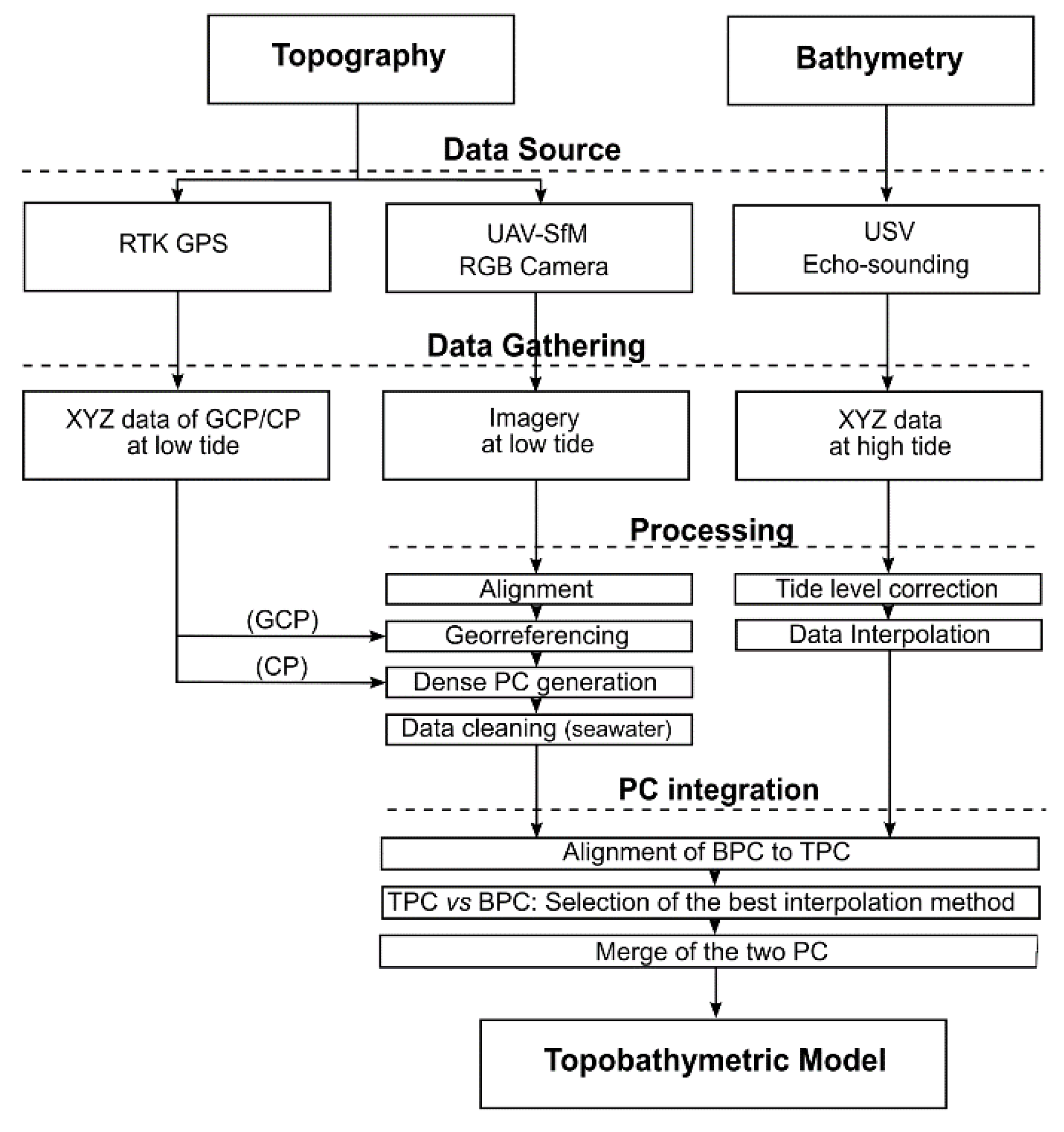
The main stages for developing the topobathymetric model are summarized in the flowchart in Figure 2.
3.1. Topography
3.1.1. Data Acquisition
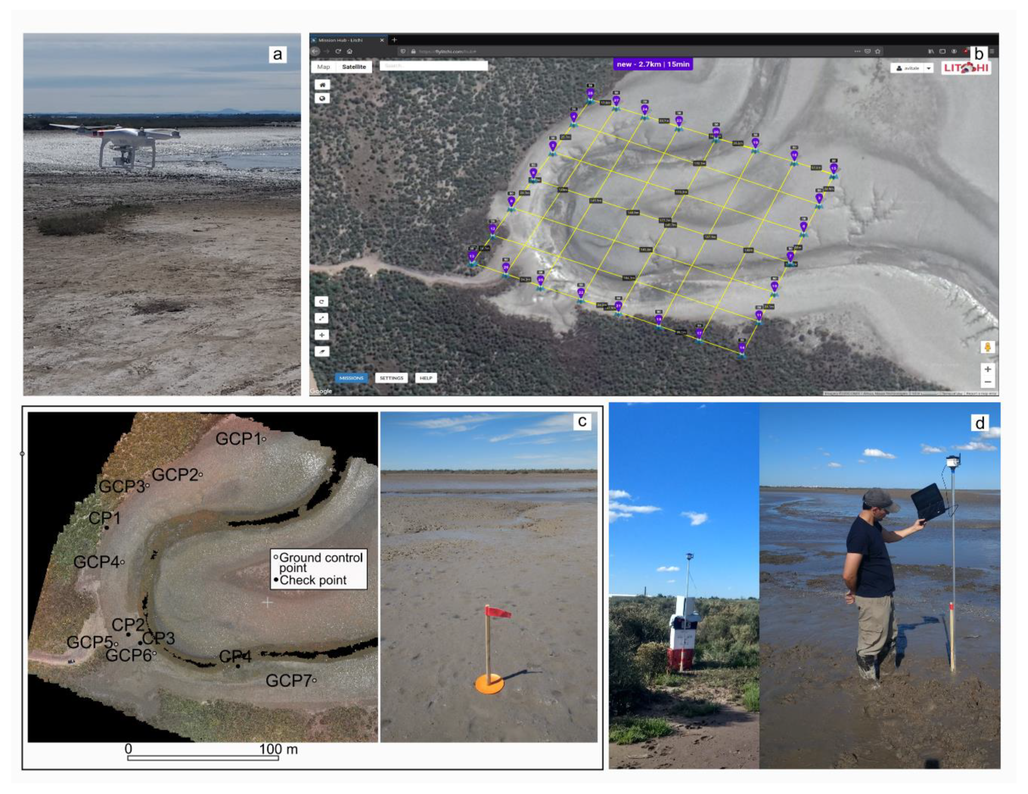
SfM-photogrammetry was used to generate the topography from suitable imagery. A DJI Phantom 3 standard quadcopter was used to capture RGB images of large size (4000 px × 3000 px) (Figure 3a). The flight was performed under optimum weather conditions (clear sky and wind speed less than 6 m s−1), in November 2018. In order to cover a larger area (i.e., non-flooded condition), the flight was made at low tide level during spring tide. To ensure a high degree of overlap, the flight path was designed as straight flight lines sampling a 30 × 30 m grid pattern (Figure 3b), over a surface of approximately 30,000 m2, at an average height of 70 m above ground level. The flight path was prepared using the commercial software Litchi (VC Technology Ltd, UK). The flight speed was set at 3 m s−1, and the images were taken every 2 s. The total survey time was 20 min.
3.1.2. Data Processing
The common steps in the standard SfM algorithm consist of the following: (i) feature detection, feature matching, and photo alignment; (ii) sparse reconstruction and bundle adjustment; (iii) dense point cloud generation; and (iv) elevation model and orthomosaic reconstruction. All of these steps are detailed in the literature [31,32]. The whole processing was performed by using Agisoft PhotoScan software. In this study, the high setting was chosen to get the best possible photo alignment accuracy and dense point cloud quality. The SfM algorithm was executed on a personal computer equipped with Intel i7 Quad Core and 8GB of memory. Once built, the dense point cloud was carefully cleaned, removing unsafe points, such as edge regions and water regions. With respect to the latter, in waters where the turbidity is high enough, as in this case, the SfM algorithm will fail to produce a successfully 3D reconstruction.
3.1.3. Indirect Georeferencing and Accuracy
The navigation system of the UAV used in this study has a low level of accuracy (vertical: ±0.5 m, horizontal: ±1.5 m) that is not acceptable for direct georeferencing. Therefore, ground control points (GCPs) were necessary to define the coordinate reference system. In this study, seven well-distributed GCPs were measured on highly visible markers in the study area immediately prior to flight (Figure 3c). It was not possible to get a large number of control points, not just because of the difficult accessibility of the study area, but also because of the susceptibility to human disturbances given the condition of protected area. The GCPs were measured by using a real-time kinematic (RTK) GPS Piksi, which is a low-cost alternative carrier phase RTK with centimeter-level relative positioning accuracy (Figure 3d). The RTK GPS base station was located over a known point previously determined with a Sokkia Radian IS operating in static mode (Figure 3d, left). The georeferencing was carried out by using Agisoft PhotoScan software. At the same time, in order to assess the accuracy of the SFM model, four checkpoints (CPs) were measured in the study area, using the RTK GPS Piksi immediately prior to flight (Figure 3c). Both sets of CPs and model coordinates (WGS 84, UTM zone 20S) were then compared to each other to determine the spatial quality in the horizontal and vertical planes.
3.2. Bathymetry
3.2.1. Data Acquisition
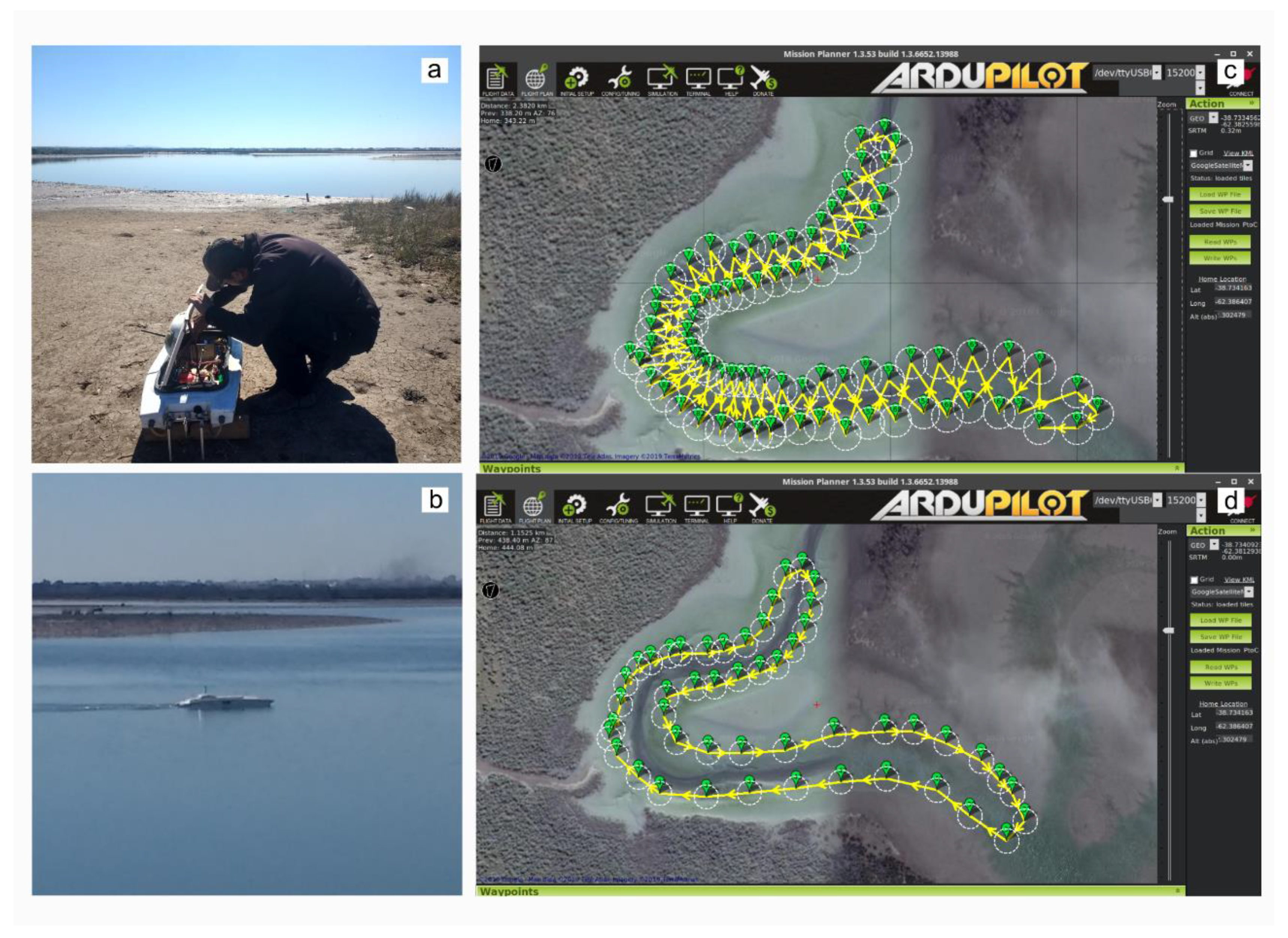
The bathymetry was performed by using a low-cost USV (Figure 4a,b; Table 1). The USV, developed by Alejandro J. Vitale (2014), at the Argentine Institute of Oceanography, is based on the Arduino open electronic platform (Ardupilot; https://ardupilot.org/). The vehicle is fitted out with an autopilot system and echo sounder, using a Garmin Echo 100 (Garmin International Inc., Olathe, KS, USA) transducer that operates at 200 kHz. The echo sounder system is integrated with a Mission Planner software to monitor the echo sounder profile during the field work. All data (i.e., GPS, acoustic profile and navigation parameters) are saved on a memory card on board at 5 Hz.
A continuous and consistent survey is critical to the quality of the bathymetry [33]. Data sampling is typically performed as either zig-zag or parallel to the centerline of the channel [34]. In this study, a zig-zag (round-trip) trajectory was performed, giving an argyle pattern to cover as much area as possible (Figure 4c). Moreover, a parallel trajectory was performed (Figure 4d). The USV moved at a constant speed of 1 m s−1, to ensure an equidistant and optimal sampling (5 points per meter) over a surface of approximately 12,000 m2. The total survey time was 35–40 min. The survey was carried out during high spring tide and optimum wind (wind speed less than 5 m s−1) and wave conditions (Figure 4a,b), in January 2019.
3.2.2. Data Processing and Accuracy
Corrections for tides at measurement time were made, using data from the tidal reference station at Ingeniero White Port, located less than 10 km from the study area (Figure 1). Tide level was measured every 2 min by using a Valeport tide gauge. The 0 m level corresponds to that of Argentine Naval Hydrographic Service.
Bathymetric point cloud (BPC) is very sparse compared to that of the topographic model. Therefore, interpolation is required to increase the point cloud density. In this study, the most commonly used interpolation methods in bathymetric mapping, such as inverse distance weighting (IDW), kriging (K), natural neighbor (NaN) and minimum curvature (MC), were considered. The Surfer software was implemented in the data interpolation procedure. Accuracy of each interpolated BPC was assessed against the reference data (i.e., georeferenced TPC) by using typical accuracy measures that consider different aspects of prediction accuracy: root mean square error (RMSE), mean average error (MAE), and coefficient of determination (R2). These statistical measurements are described by the following equations:
where pi is the estimated value by using a specific interpolator at point i, and ai is the actual value at the same point. For this, R software was used. To assess the accuracy, each interpolated BPC set was aligned to the TPC by means of an iterative closest point algorithm, since a conversion of source elevation data to a given vertical datum is required to avoid errors and discontinuities. Final bathymetric data were obtained based on the best interpolation result. Before merging both TPC and BPC, overlapping points were removed from the interpolated BPC, in order to keep only the region of points on the low tide level. Alignment and merging of the two point clouds were performed by using CloudCompare software.
4. Results and Discussion
4.1. SfM Topography: Derivation and Accuracy
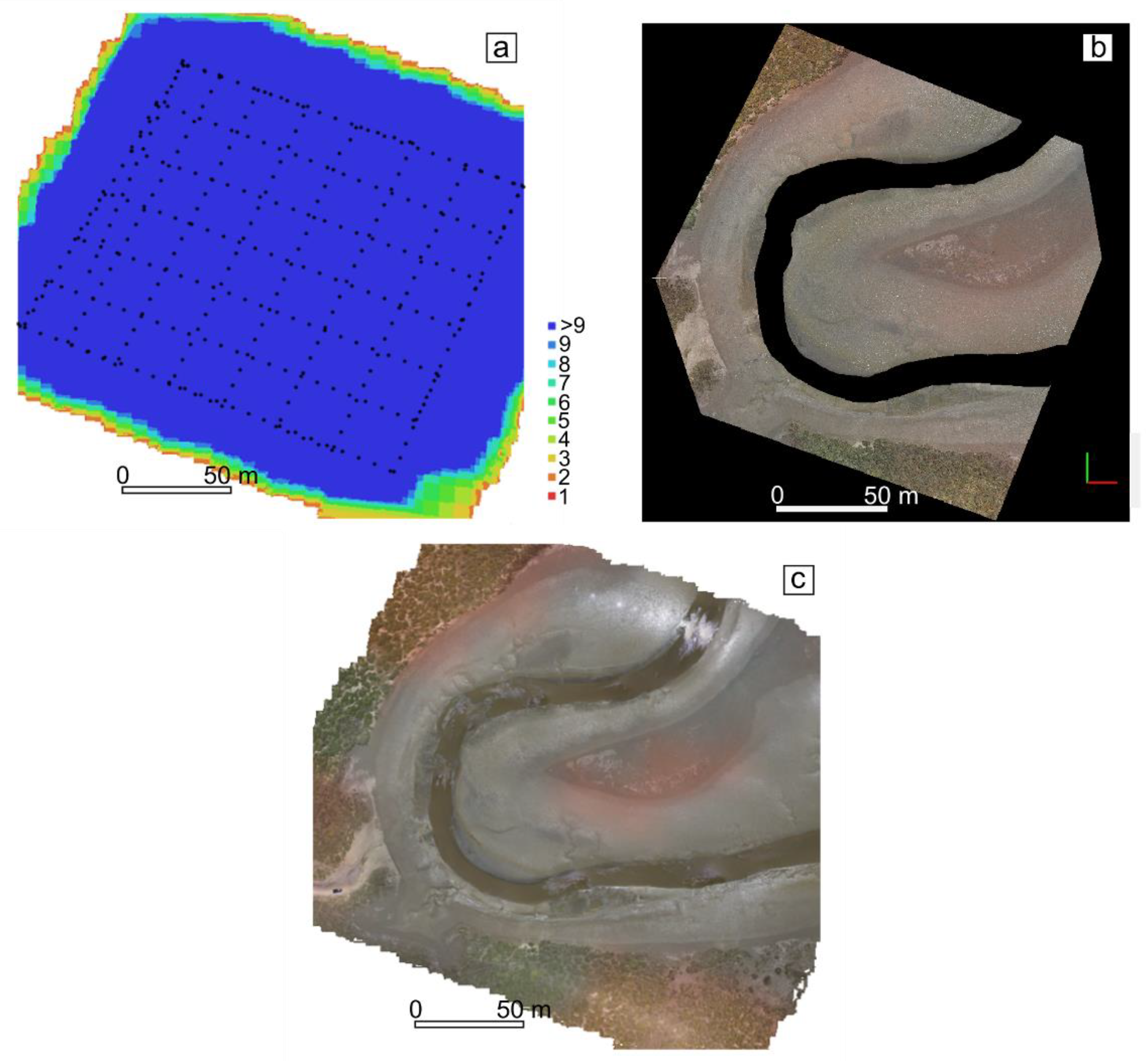
A total of 380 images were used to generate the SfM model. An adequate overlap of the images was achieved, as can be seen in Figure 5a. Figure 5b shows the cleaned dense point cloud (or TPC) with its RGB data. The resultant TPC has a density of about 1200 points per square meter. The model, after accounting for mosaicking and orthorectification processes, has a resolution of 3.6 cm/px. A visual inspection of the orthomosaic reveals that undesired morphologic features were not detected and that the color balancing was good except for the sunshine effect in a small portion of the water remnant flowing into the tidal channel (Figure 5c). The total computer time required for obtaining the SfM reconstruction was 19 h.
The accuracy of the indirect georeferencing was calculated by Agisoft PhotoScan software, from the differences between the x, y, and z coordinates of the seven GCPs measured by RTK GPS, and their coordinates pointed out on the SfM model (Table 2, upper part). The RMSE of the model with seven GCPs was 0.15 and 0.13 m in the x and y coordinates, respectively, and 0.07 m vertically. The accuracy of the SfM model at each CP measured by the RTK DGPS is presented in Table 2 (lower part). The RMSE was 0.10 and 0.06 m in the x and y coordinates, respectively, and 0.09 m vertically. The mean absolute value (MAV), which is obtained from the average of the absolute value of each CP error, was about 0.07 and 0.08 m for the horizontal and vertical planes, respectively. In particular, it is important to highlight that the vertical MAV and RMSE values were lower for GCPs than for CPs, which was crucial for ensuring an adequate photogrammetric output. According to the literature review carried out by Andersen [20], the vertical accuracy of conventional topographic LiDAR data varies, ranging from ±0.10 to ±0.15 m. Therefore, in this study, the accuracy values are similar in comparison with previous studies.
4.2. Bathymetry Accuracy
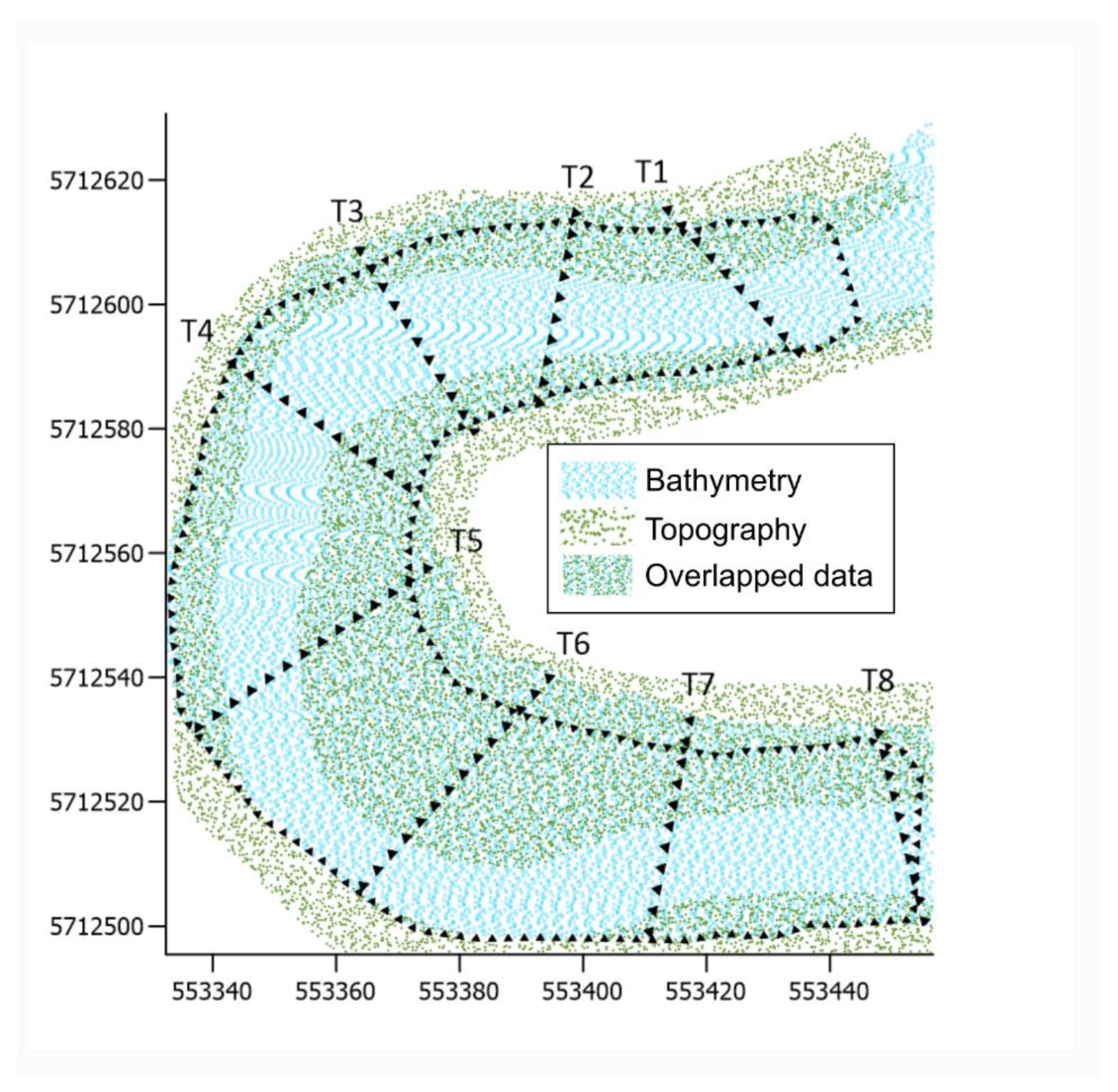
The accuracy of interpolated bathymetric datasets using most common interpolation methods was performed against the reference TPC, along the random transects and the perimeter in the overlapping region (Figure 6 and Table 3). Combinations of interpolation parameters (e.g., search, smoothing factor, etc.) were previously evaluated by using cross-validation and visual examination, to avoid artifacts in the interpolated surface. In addition, the accuracy is affected by the spacing of the interpolation grid, making it an essential parameter [35]; therefore, grid spacing at 0.25 and 0.50 m was assessed.
In average terms, the IDW interpolation method (power parameter: 1, smoothing factor: 2, number of neighborhoods: 8) showed the best RMSE (0.18 m) and MAE (0.05 m) values among all considered methods (Table 3). Moreover, IDW method had the highest values of R2 (0.90) (Table 3). This may be due to the sampling pattern, which is characterized by samples with sufficient spatial regularity covering a large portion at a density of 2–3 points per square meter. The grid spacing at 0.50 m showed the best results for all methods. K and NaN methods gave similar results (RMSE ≈ 0.21 m; MAE ≈ 0.09 m). The worst results were obtained with the MC method (RMSE ≈ 0.25 m; MAE ≈ 0.11 m). A comparison with other studies is not feasible, since there is no consensus about which interpolation method performs the best in generating bathymetric surfaces [36,37]. The performance of the interpolated datasets along the random transects indicates that there is no spatial trend across the study area (Table 3).
4.3. Final Topobathymetric Model
The final obtained topobathymetric model, illustrated in Figure 7, has a spatial resolution of approximately 8 cm (TPC) and 50 cm (BPC). Here, it is interesting to remember that the accuracy results of the topobathymetric model gave an RMSE value of 0.09 m (topography) and an RMSE of 0.18 m and a MAE of 0.05 (bathymetry) for the vertical plane. The few studies that provide accuracy topobathymetry in shallow coastal waters used LiDAR technology, and they reported values from ±0.04 m [20] to ±0.10–0.14 m [25]. Therefore, our results are in line with these studies, but using different methodology and cheaper technology.
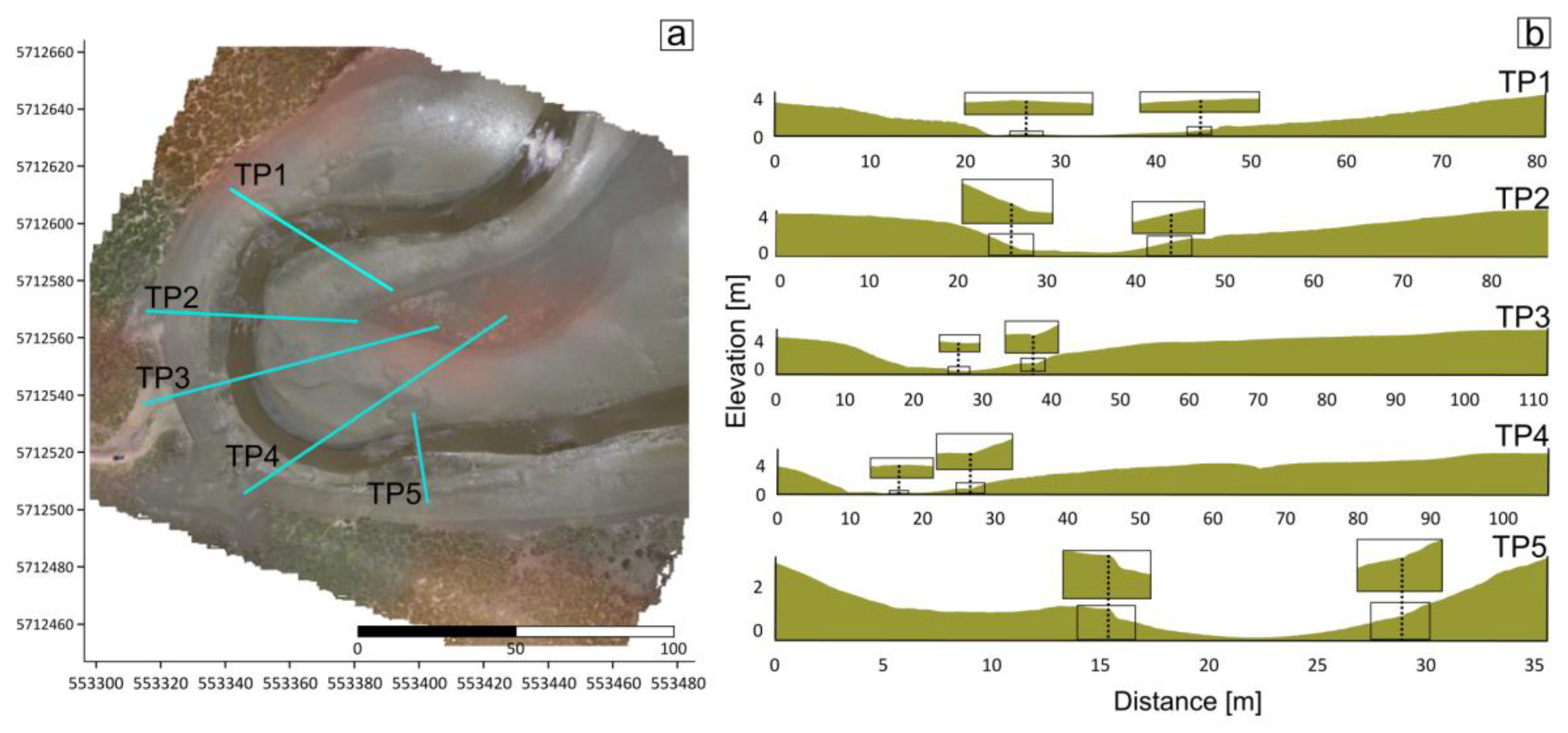
The topobathymetric model retains a clear definition of many terrain features. For instance, several types of tidal courses that are present in the study area [38], such as a channel, a creek (width: 10–200 cm and depth: 10–200 cm), and gullies (width: 10–100 cm and depth: 5–100 cm), are well represented in the model (Figure 7c). The exceptions are tidal rills and grooves (widths less than 2–10 cm and depths less than 1–5 cm), and crab burrows—crab Neohelice granulata—(depth usually less than 5 cm), which require a higher spatial resolution to be obtained. Another feature observed is the presence of little exposed rock on the bottom channel. Regarding the subtidal zone, both 3D-perspective view of the model (Figure 7b) and transverse profiles (Figure 8) exhibit a flat bottom in the U-shape form, as would be expected in shallow environments. It can be seen that the transverse topobathymetric profiles from Figure 8 show a good transition between TPC and BPC, despite the differences in their data (density, reference plane, etc.).
4.4. Cross-Analysis of the Topobathymetric and Tidal Data
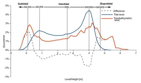
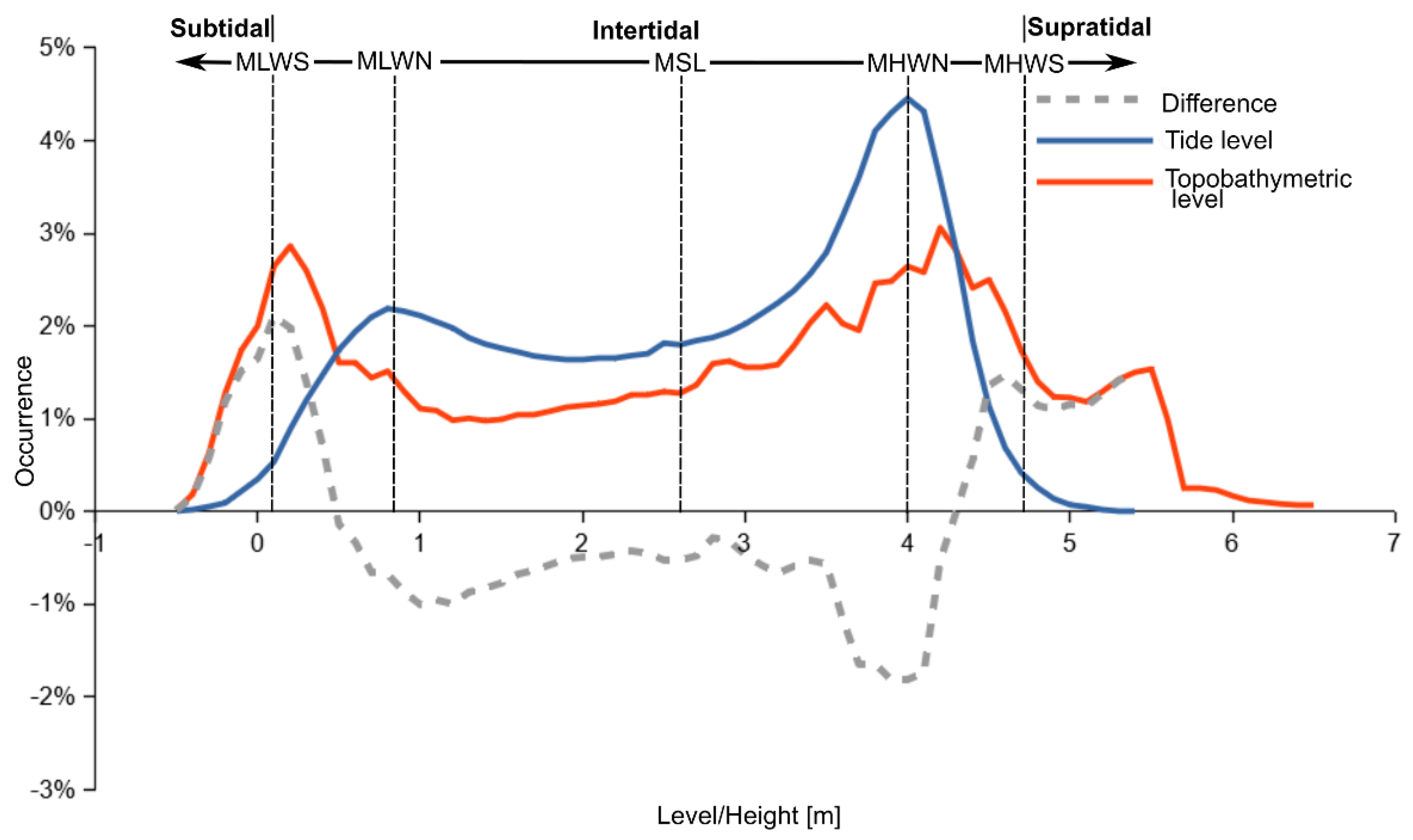
Figure 9 shows the frequency plots belonging to the tide level at Ingeniero White Port for ten years (2010–2019) and the topobathymetric levels for the study area. Both plots were considered together, for easy comparison. For this purpose, the topobathymetric data were referred to the datum plane of Ingeniero White Port. The terms mean high/low water spring (MHWS and MLWS) and mean high/low water neaps (MHWN and MLWN) apply only to those regions with a semidiurnal regime [39,40], as in this case, as seen in Figure 9 and Figure 10. Spring tides mark the limit between supratidal, intertidal, and subtidal hydrogeomorphic zones [41] (Figure 9 and Figure 10).
The tide level exhibits a bimodal distribution with peaks at about 0.8 (MLWN) and 4.0 m (MHWN). The peak that corresponds to high tides is notably higher than the low tide peak, indicating a large diurnal inequality. According to the tide gauge data, the flooding by tidal water of the supratidal zone (water levels more than 4.7 m) happens 0.97% of the time (i.e., a total of about 85 h a year) (Figure 9); in contrast, subaerial exposure with water levels less than 0.1 m happens 1.28% of the time (i.e., a total of about 112 h a year) (Figure 9). These results are associated with the findings of Perillo and Piccolo [42], who studied the deviations of the tide levels from the predicted astronomical tides at Ingeniero White Port. They found maximum values larger than 2 m which coincide with the winds blowing from the NW (predominant direction) and from the SW. The latter are intense wind events that are related to the local phenomenon called sudestada, whose effect is stronger when it coincides with the high tide.
The frequency plot of the topobathymetric levels exhibits two large peaks, corresponding to the subtidal channel (values centered at about 0 m) and to the edge of the upper intertidal zone (values centered at about 4.5 m) (Figure 9). Moreover, a noticeable peak at about 5.5 m is observed, which corresponds to a small elevated island (Figure 9 and Figure 10e). According to the topobathymetric data, the supratidal zone occupies 5% of the study area, while the subtidal zone occupies 8.5% (Figure 9 and Figure 10). However, it should be remembered that a large portion of the supratidal zone (vegetated by halophytic shrubs) was removed from the analysis. The remaining intertidal zone occupies 76.5% of the study area (Figure 9 and Figure 10). It is interesting to note that both peaks of tide level remain inside the largest peaks of topobathymetry, as was expected (Figure 9).
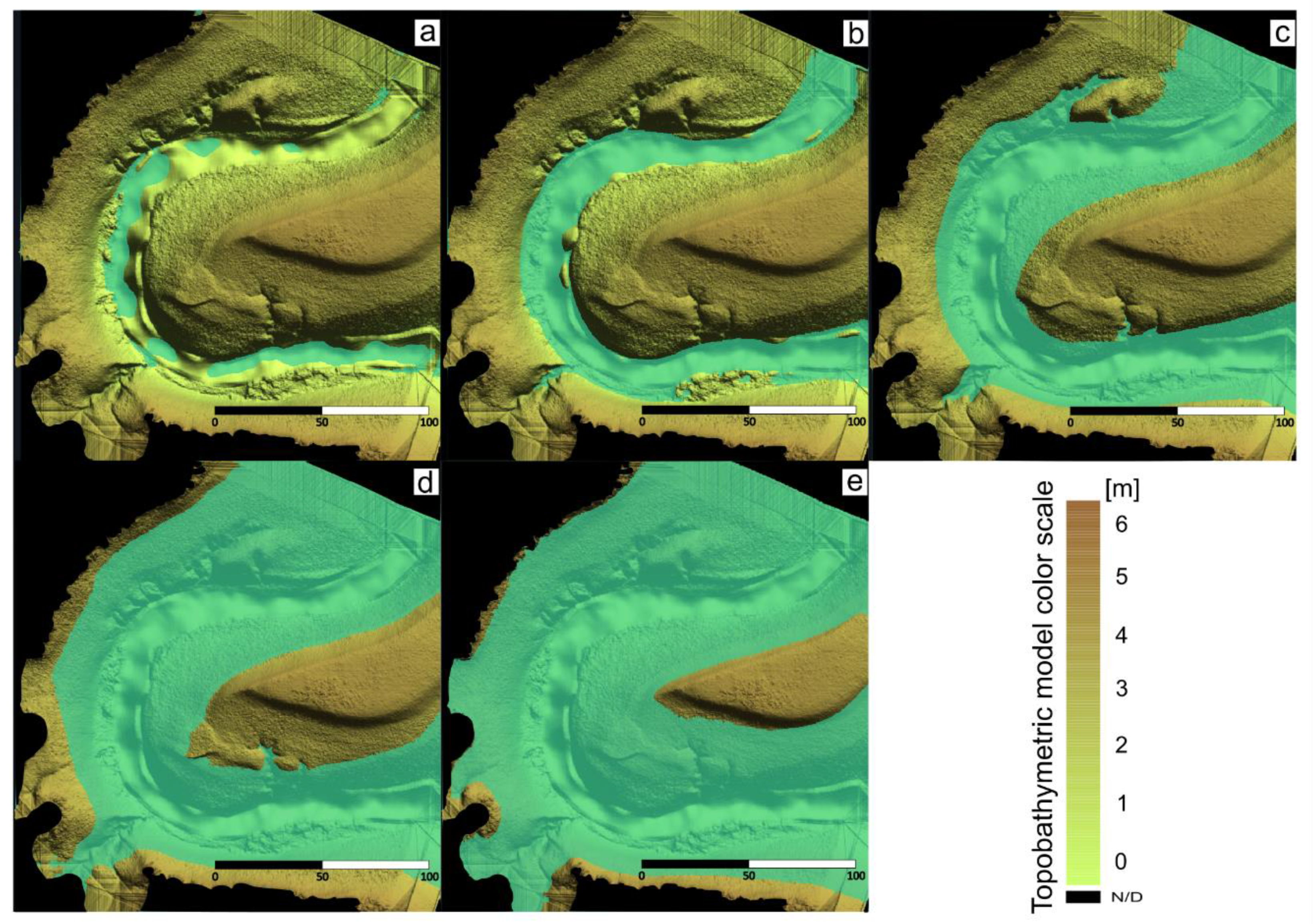
In particular, Figure 10a,b, which illustrates the topobathymetric model at low tide conditions (i.e., MLWN and MLWS), allows us to identify the different tidal courses according to Perillo [38], who defined the water in low tide level as one of the criteria for classifying them. Thus, courses containing tidal water, such as the tidal channel and one creek (Figure 7c), can be clearly identified. Unlike these tidal courses, the gullies, which have a significant presence, are not reached by the tidal inundation at low tide levels.
4.5. Advantages, Limitations and Applications of Topobathymetry
There are limitations and challenges for carrying out topobathymetric surveys in coastal regions. Firstly, these environments involve flooded and non-flooded areas that require specific survey needs in terms of technology and methods, as reflected in this study. Besides, it is well-known that these regions are hydrodynamically complex. This complexity is given partly by the multiplicity of periods on which the tide varies, but also by the seasonal, but otherwise random, frequently significant influence of storm surges [39,43]. In this regard, topographic and bathymetric surveys are subject to the stage of the tidal level (e.g., spring/neap tides and high/low tide level). For example, in this study, topographic and bathymetric surveys were carried out during spring tidal conditions, at low and high tide, respectively, to ensure larger sampling areas. The daily tidal cycle of high and low tides leads to a short surveying time that must be taken into account when preparing the field campaign. In another study, Jaud et al. [8] outlined similar challenges for monitoring mudflat morphodynamics, but they only focused on topographic surveys using SfM.
Regarding the wave conditions, its non-uniform behavior in shallow waters causes inaccuracy in the bathymetry that requires further corrections. In particular, estuaries, lagoons, or enclosed embayments are fetch-limited environments that are protected from ocean-generated waves [44], minimizing the wave effect. In regard to the current study, it should be remembered that the bathymetry survey was carried out in an area where waves are generally fetch-limited; besides, the survey was carried out under optimum wind and wave conditions (wind speed less than 5 m s−1; Figure 4a,b).
Boat-based surveys in shallow (depths between 1 and 10 m) and very shallow (depth less than 1 m) waters are difficult or sometimes even impossible to overcome due to problems related to maneuvering performance [45]. Operations in these shallow environments require the draft to be low and that there be a protection mechanism for the propellers, just like the USV [46]. The shallow draft of the USV used in this study is 0.15 m, which enables it to carry out bathymetric surveys in very shallow waters in a suitable way; thus, the platform allows a wide range of depths, from 0.3 to 100 m, to be covered. Another aspect of interest is that the maneuvering performance in narrow tidal courses is controlled by the minimum turning radius of the platform, which is 2.5 m in this case. Path planning becomes a crucial factor for USV’s control system that deserves special attention in shallow/very shallow waters, as well as in narrow tidal courses.
Table 4 summarizes the costs and characteristics of the survey equipment that was used in this study. The total cost of the survey equipment, including the RTK GPS, was approximately US $2500. The autonomy, which is expressed by the battery capacity, is low for UAV (15–20 min), thereby affecting the flight time; in contrast, with regard to the USV, because of its design (storage capacity) and its high paid load (Table 1), it can reach an operation time by approximately more than one order of magnitude compared to UAV. The survey rate is higher for the UAV (≈ 0.16 km2 h−1 at 70 m height) than for the USV (≈ 0.06 km2 h−1).
The working conditions, such as atmosphere state and water level, are far more demanding for unmanned platforms than for RTK GPS (Table 4). The wind speed is the most critical parameter impacting directly on the UAV and indirectly on the USV (wind-generated gravity waves), putting them at risk of being damaged or lost. An advantage of shallow environments is that they are not affected by shadows from elevated features which are unfavorable for generating of image-based point clouds. When UAV images are taken under partially cloudy skies, the SfM algorithm would fail due to the cloud shadow effect, especially in homogeneous regions. Cloudy skies can also make RTK GPS surveys difficult or unreliable, especially when high accuracy is required.
The complexity varies from one equipment to another (Table 4). In relative terms, the UAV is the simplest for the operational stage, but it acquires the greatest complexity in the post-processing stage, since it involves the most time-consuming, computationally intensive, and critical part (e.g., indirect georeferencing process), as was detailed in the flowchart in Figure 2. In contrast, the USV is simple in the post-processing stage, but it is slightly more complex than the UAV in terms of operational stage, since it requires careful maneuvering, mainly in shallow and narrow water bodies. The unmanned platforms are generally designed to be used by a single person, while the RTK GPS must be performed by at least two persons, especially in muddy estuarine environments, as in this study, and requires more expertise and time-consuming work (e.g., base station definition, setting tasks, etc.).
It is well-known that, compared to ground-based techniques, the unmanned platforms allow non-destructive and non-invasive surveys. In contrast, the use of RTK GPS, which is performed by walking across each of the fixed points (GCP and CP), can cause damage to estuarine habitats. The latter can be overcome by using UAV equipped with high-accuracy RTK GPS, but it is an expensive option, since its cost is two-to-three times higher than that of the whole equipment used in this study.
Regarding the applicability of the proposed methodology under different coastal conditions, wave disturbance is presented as the most important obstacle, in which the significant vessel motion caused by wave action affects the bathymetric survey. In order to solve this issue, an option is to put on board the RTK GPS Piksi and to use its vertical positioning data during the post-processing correction stage. If necessary, the IMU (Inertial Measurements Unit) data from Ardupilot can be used to improve post-processing correction. It should be noted that the technology on board the USV (GPS, echo sound system, and autopilot; Table 1) can be migrated to a more suitable platform in terms of size and power, in a reliable and relatively cheap way, in order to work properly under different forcing factors (e.g., strong winds and extreme sea/river currents). Therefore, considering all mentioned above, the methodology can be adapted to different conditions and environments, with a non-significant increase in costs.
5. Conclusions
In this study, a methodology to generate a topobathymetric model in a shallow/very shallow and turbid tidal environment, using low-cost equipment, was presented. As a main conclusion, a continuous terrain model was built with a spatial resolution of approximately 0.08 (TPC) and 0.50 m (BPC). With respect to the TPC, the accuracy of the SfM gave a RMSE value of 0.09 m for the vertical plane. The best interpolated BPC (IDW method, grid spacing at 0.50 m), which was aligned to the TPC (as reference), showed on average an RMSE of 0.18 m and a MAE of 0.05 m. Our results are in line with other findings, but using different methodology and cheaper technology.
The final topobathymetric model showed an adequate representation of the terrain, making it well suited for examining many landforms. Tidal forms that are present in the study area, such as a channel, a creek, gullies, and U-shaped bottoms, among others, were well identified in the model. As was expected, other small forms, such as tidal rills or grooves and crab burrows with depths usually less than 5 cm, could not be identified, highlighting a scale issue that could be explored in future studies. In addition to this, for modeling purposes, since the spatial resolution of the resultant topobathymetric model is at least four-to-five times better than that required for existing coastal models, a down-sampling procedure could be applied in order to generate a coarse grid and, therefore, to reduce the computational time and complexity.
The total cost of the survey equipment used in this study for topobathymetry was about US$ 2500, which is much less than any other alternative. Besides, there are clear advantages in using unmanned platforms, such as their high portability and non-destructive nature, which imply that they are a good alternative to traditional survey technologies. The use of UAV equipped with high-accuracy RTK GPS is actually less time-consuming, but it is also far more expensive.
This study helps to confirm the potential for remote sensing of shallow tidal environments, by demonstrating how the data source heterogeneity can be applied. Finally, the study presented here provides a framework for topobathymetric survey that applies to other environments/conditions, since the technology on board the USV can be migrated to a suitable platform, in a reliable and relatively cheap way, in order to work properly under different forcing factors.
Author Contributions
Conceptualization, S.A.G.; methodology, S.A.G. and A.J.V.; data acquisition: S.A.G. and A.J.V.; formal analysis, S.A.G. and A.J.V.; writing—original draft preparation, S.A.G.; writing—review, S.A.G., A.J.V., and G.M.E.P.; visualization and editing, S.A.G. and C.S.; supervision, A.J.V., G.M.E.P., and C.A.D.; resources, A.J.V., G.M.E.P., and C.A.D. All authors have read and agreed to the published version of the manuscript.
Funding
This research was funded by ANPCyT, grant number PICT-2012-1065, and by Universidad Nacional del Sur, grant number VT42-UNS11741.
Acknowledgments
The authors would like to thank Ing. Gian Marco Mavo Manstretta for the help in the field data collection. The authors are grateful for the provision of tide gauge data by the Bahía Blanca Port Consortium.
Conflicts of Interest
The authors declare no conflict of interest.
References
- Cicin-Sain, B.; Knecht, R.W.; Jang, D.; Knecht, R.; Fisk, G.W. Integrated Coastal and Ocean Management: Concepts and Practices; Island Press: Washington, DC, USA, 1998; p. 491. [Google Scholar]
- Alvarez, L.V.; Moreno, H.A.; Segales, A.R.; Pham, T.G.; Pillar-Little, E.A.; Chilson, P.B. Merging Unmanned Aerial Systems (UAS) Imagery and Echo Soundings with an Adaptive Sampling Technique for Bathymetric Surveys. Remote Sens. 2018, 10, 1362. [Google Scholar] [CrossRef] [Green Version]
- Bergsma, E.W.J.; Conley, D.C.; Davidson, M.A.; O’Hare, T.J. Video-based nearshore bathymetry estimation in macro-tidal environments. Mar. Geol. 2016, 374, 31–41. [Google Scholar] [CrossRef] [Green Version]
- Jagalingam, P.; Akshaya, B.J.; Hegde, A.V. Bathymetry mapping using Landsat 8 satellite imagery. Procedia Eng. 2015, 116, 560–566. [Google Scholar] [CrossRef] [Green Version]
- Genchi, S.A.; Vitale, A.J.; Perillo, G.M.E.; Delrieux, C.A. Structure-from-Motion approach for characterization of bioerosion patterns using UAV imagery. Sensors 2015, 15, 3593–3609. [Google Scholar] [CrossRef] [PubMed] [Green Version]
- Kääb, A.; Girod, L.; Berthling, I. Surface kinematics of periglacial sorted circles using structure-from-motion technology. Cryosphere 2014, 8, 1041–1056. [Google Scholar] [CrossRef] [Green Version]
- Mancini, F.; Dubbini, M.; Gattelli, M.; Stecchi, F.; Fabbri, S.; Gabbianelli, G. Using Unmanned Aerial Vehicles (UAV) for High-Resolution Reconstruction of Topography: The Structure from Motion Approach on coastal environments. Remote Sens. 2013, 5, 6880–6898. [Google Scholar] [CrossRef] [Green Version]
- Jaud, M.; Grasso, F.; Le Dantec, N.; Verney, R.; Delacourt, C.; Ammann, J.; Deloffre, J.; Grandjean, P. Potential of UAVs for Monitoring Mudflat Morphodynamics (Application to the Seine Estuary, France). ISPRS Int. J. Geo-Inform. 2016, 5, 50. [Google Scholar] [CrossRef] [Green Version]
- Long, N.; Millescamps, B.; Guillot, B.; Pouget, F.; Bertin, X. Monitoring the Topography of a Dynamic Tidal Inlet Using UAV Imagery. Remote Sens. 2016, 8, 387. [Google Scholar] [CrossRef] [Green Version]
- Esposito, G.; Salvini, R.; Matano, F.; Sacchi, M.; Danzi, M.; Somma, R.; Troise, C. Multitemporal monitoring of a coastal landslide through SfM-derived point cloud comparison. Photogramm. Rec. 2017, 32, 459–479. [Google Scholar] [CrossRef] [Green Version]
- Pagán, J.I.; Bañón, L.; López, I.; Bañón, C.; Aragonés, L. Monitoring the dune-beach system of Guardamar del Segura (Spain) using UAV, SfM and GIS techniques. Sci. Total Environ. 2019, 687, 1034–1045. [Google Scholar] [CrossRef]
- Guisado-Pintado, E.; Jackson, D.W.T.; Rogers, D. 3D mapping efficacy of a drone and terrestrial laser scanner over a temperate beach-dune zone. Geomorphology 2019, 328, 157–172. [Google Scholar] [CrossRef]
- Tonkin, T.N.; Midgley, N.G.; Graham, D.J.; Labadz, J.C. The potential of small unmanned aircraft systems and structure-from-motion for topographic surveys: A test of emerging integrated approaches at Cwm Idwal, North Wales. Geomorphology 2014, 226, 35–43. [Google Scholar] [CrossRef] [Green Version]
- Gesch, D.B.; Brock, J.C.; Parrish, C.E.; Rogers, J.N.; Wright, C.W. Introduction: Special Issue on Advances in Topobathymetric Mapping, Models. J. Coast. Res. 2016, 76, 1–3. [Google Scholar] [CrossRef]
- Collin, A.; Hench, J.L.; Pastol, Y.; Planes, S.; Thiault, L.; Schmitt, R.J.; Holbrook, S.J.; Davies, N.; Troyer, M. High resolution topobathymetry using a Pleiades-1 triplet: Moorea Island in 3D. Remote Sens. Environ. 2018, 208, 109–119. [Google Scholar] [CrossRef]
- Gesch, D.; Wilson, R. Development of a seamless multisource topographic/bathymetric elevation model of Tampa Bay. Mar. Technol. Soc. J. 2001, 35, 58–64. [Google Scholar] [CrossRef] [Green Version]
- Quadros, N.D.; Collier, P.A.; Fraser, C.S. Integration of Bathymetric and Topographic LiDAR: A Preliminary Investigation. ISPRS Arch. 2008, 37, 1299–1304. [Google Scholar]
- Eakins, B.W.; Grothe, P.R. Challenges in building coastal digital elevation models. J. Coast. Res. 2014, 30, 942–953. [Google Scholar] [CrossRef] [Green Version]
- Danielson, J.J.; Poppenga, S.K.; Brock, J.C.; Evans, G.A.; Tyler, D.J.; Gesch, D.B.; Thatcher, C.A.; Barras, J.A. Topobathymetric elevation model development using a new methodology: Coastal national elevation database. J. Coast. Res. 2016, 76, 75–89. [Google Scholar] [CrossRef] [Green Version]
- Andersen, M.S.; Gergely, Á.; Al-Hamdani, Z.; Steinbacher, F.; Larsen, L.R.; Ernstsen, V.B.J.H.; Sciences, E.S. Processing and performance of topobathymetric lidar data for geomorphometric and morphological classification in a high-energy tidal environment. Hydrol. Earth Syst. Sci. 2017, 21, 43–63. [Google Scholar] [CrossRef] [Green Version]
- Ojeda Zújar, J.; Álvarez Francoso, J.I.; Fraile Jurado, P.; Márquez Pérez, J.; Sánchez Rodríguez, E. Gestión e integración de datos altimétricos y batimétricos en la costa andaluza: El uso del “model builder”. In Tecnologías de la Información Geográfica: La Información Geográfica al Servicio de los Ciudadanos; Ojeda, J., Pita, M.F., Vallejo, I., Eds.; Secretariado de Publicaciones de la Universidad de Sevilla: Sevilla, Spain, 2010; pp. 956–970. [Google Scholar]
- Feyen, J.; Hess, K.; Spargo, E.; Wong, A.; White, S.; Sellars, J.; Gill, S. Development of a continuous bathymetric/topographic unstructured coastal flooding model to study sea level rise in North Carolina. In Proceedings of the International Conference on Estuarine and Coastal Modeling 2005, Charleston, SC, USA, 31 October–2 November 2005; Spaulding, M.L., Ed.; ASCE: Reston, VA, USA, 2006; pp. 338–356. [Google Scholar]
- Foxgrover, A.C.; Finlayson, D.P.; Jaffe, B.E. Bathymetry and Digital Elevation Model of Coyote Creek and Alviso Slough, South San Francisco Bay; U.S. Geological Survey: Reston, CA, USA, 2011; p. 23. [CrossRef]
- Medeiros, S.C.; Ali, T.A.; Hagen, S.C.; Raiford, J.P. Development of a seamless topographic/bathymetric digital terrain model for tampa bay, Florida. Photogramm. Eng. Remote Sens. 2011, 77, 1249–1256. [Google Scholar] [CrossRef]
- Nayegandhi, A.; Brock, J.C.; Wright, C.W. Small-footprint, waveform-resolving lidar estimation of submerged and sub-canopy topography in coastal environments. Int. J. Remote Sens. 2009, 30, 861–878. [Google Scholar] [CrossRef]
- Perillo, G.M.E.; Piccolo, M.C.; Parodi, E.; Freije, R.H. The Bahia Blanca Estuary, Argentina. In Coastal Marine Ecosystems of Latin America. Ecological Studies (Analysis and Synthesis); Seeliger, U., Kjerfve, B., Eds.; Springer: Berlin/Heidelberg, Germany, 2001; Volume 144, pp. 205–217. [Google Scholar] [CrossRef]
- Popovich, C.A.; Marcovecchio, J.E. Spatial and temporal variability of phytoplankton and environmental factors in a temperate estuary of South America (Atlantic coast, Argentina). Cont. Shelf Res. 2008, 28, 236–244. [Google Scholar] [CrossRef]
- Perillo, G.M.E.; Piccolo, M.C. Geomorphologic and physical characteristics of the Bahía Blanca Estuary. Argentina. In Estuaries of South America: Their Geomorphology and Dynamics; Environmental Science Series; Perillo, G.M.E., Piccolo, M.C., Pino Quivira, M., Eds.; Springer: Berlin/Heidelberg, Germany, 1999; pp. 195–216. [Google Scholar]
- Perillo, G.M.E.; Iribarne, O.O. Processes of tidal channels develop in salt and freshwater marshes. Earth Surf. Process. Landf. 2003, 28, 1473–1482. [Google Scholar] [CrossRef]
- Escapa, C.M.; Minkoff, D.R.; Perillo, G.M.E.; Iribarne, O.O. Direct and indirect effects of burrowing crab activities on erosion of Southwest Atlantic Sarcocornia-dominated marshes. Limnol. Oceanogr. 2007, 52, 2340–2349. [Google Scholar] [CrossRef]
- Jaud, M.; Passot, S.; Le Bivic, R.; Delacourt, C.; Grandjean, P.; Le Dantec, N. Assessing the accuracy of high resolution digital surface models computed by PhotoScan® and MicMac® in sub-optimal survey conditions. Remote Sens. 2016, 8, 465. [Google Scholar] [CrossRef] [Green Version]
- James, M.R.; Robson, S.; d’Oleire-Oltmanns, S.; Niethammer, U. Optimising UAV topographic surveys processed with structure-from-motion: Ground control quality, quantity and bundle adjustment. Geomorphology 2017, 280, 51–66. [Google Scholar] [CrossRef] [Green Version]
- Chadwick Jr, W.W.; Scheirer, D.S.; Embley, R.W.; Johnson, H.P. High-resolution bathymetric surveys using scanning sonars: Lava flow morphology, hydrothermal vents, and geologic structure at recent eruption sites on the Juan de Fuca Ridge. J. Geophys. Res. Solid Earth. 2001, 106, 16075–16099. [Google Scholar] [CrossRef]
- Krüger, R.; Karrasch, P.; Bernard, L. Evaluating Spatial Data Acquisition and Interpolation Strategies for River Bathymetries. In Geospatial Technologies for All. AGILE 2018. Lecture Notes in Geoinformation and Cartography; Mansourian, A., Pilesjö, P., Harrie, L., van Lammeren, R., Eds.; Springer: Cham, Germany, 2018; pp. 3–25. [Google Scholar]
- Gosciewski, D. Selection of interpolation parameters depending on the location of measurement points. GISci. Remote Sens. 2013, 50, 515–526. [Google Scholar] [CrossRef]
- Curtarelli, M.; Leão, J.; Ogashawara, I.; Lorenzzetti, J.; Stech, J. Assessment of Spatial Interpolation Methods to Map the Bathymetry of an Amazonian Hydroelectric Reservoir to Aid in Decision Making for Water Management. ISPRS Int. J. Geo-Inform. 2015, 4, 220–235. [Google Scholar] [CrossRef]
- Wu, C.Y.; Mossa, J.; Mao, L.; Almulla, M. Comparison of different spatial interpolation methods for historical hydrographic data of the lowermost Mississippi River. Ann. GIS. 2019, 25, 133–151. [Google Scholar] [CrossRef]
- Perillo, G.M.E. Tidal Courses: Classification, Origin and Functionality. In Coastal Wetlands: An Integrated Ecosystem Approach; Perillo, G.M.E., Wolanski, E., Cahoon, D.R., Brinson, M.M., Eds.; Elsevier: Amsterdam, The Netherlands, 2009; pp. 185–209. [Google Scholar]
- Pugh, D.T. Natural Tides, Surges and Mean Sea-Level; John Wiley & Sons: New York, NY, USA, 1996; p. 486. [Google Scholar]
- Liu, X.; Xia, J.; Wright, G.; Arnold, L. A state of the art review on High Water Mark (HWM) determination. Ocean Coast. Manag. 2014, 102, 178–190. [Google Scholar] [CrossRef]
- Daidu, F.; Yuan, W.; Min, L. Classifications, sedimentary features and facies associations of tidal flats. J. Palaeogeogr. 2013, 2, 66–80. [Google Scholar] [CrossRef]
- Perillo, G.M.E.; Piccolo, M.C. Tidal Response in the Bahia Blanca Estuary, Argentina. J. Coast. Res. 1991, 7, 437–449. [Google Scholar]
- Allen, J.R.L. Sedimentary structures: Sorby and the last decade. J. Geol. Soc. Lond. 1993, 150, 417–425. [Google Scholar] [CrossRef]
- Freire, P.; Ferreira, O.; Taborda, R.; Oliveira, F.S.B.F.; Carrasco, A.R.; Silva, A.; Vargas, C.; Capitão, R.; Fortes, C.J.; Coli, A.B.; et al. Morphodynamics of Fetch-limited Beaches in Contrasting Environments. J. Coast. Res. 2009, SI 56, 183–187. [Google Scholar]
- Specht, M.; Specht, C.; Lasota, H.; Cywiński, P. Assessment of the steering precision of a hydrographic Unmanned Surface Vessel (USV) along sounding profiles using a low-cost Multi-Global Navigation Satellite System (GNSS) receiver supported autopilot. Sensors 2019, 19, 3939. [Google Scholar] [CrossRef] [Green Version]
- Demetillo, A.T.; Taboada, E.B. Real-time water quality monitoring for small aquatic area using unmanned surface vehicle. Eng. Technol. Appl. Sci. Res. 2019, 9, 3959–3964. [Google Scholar]
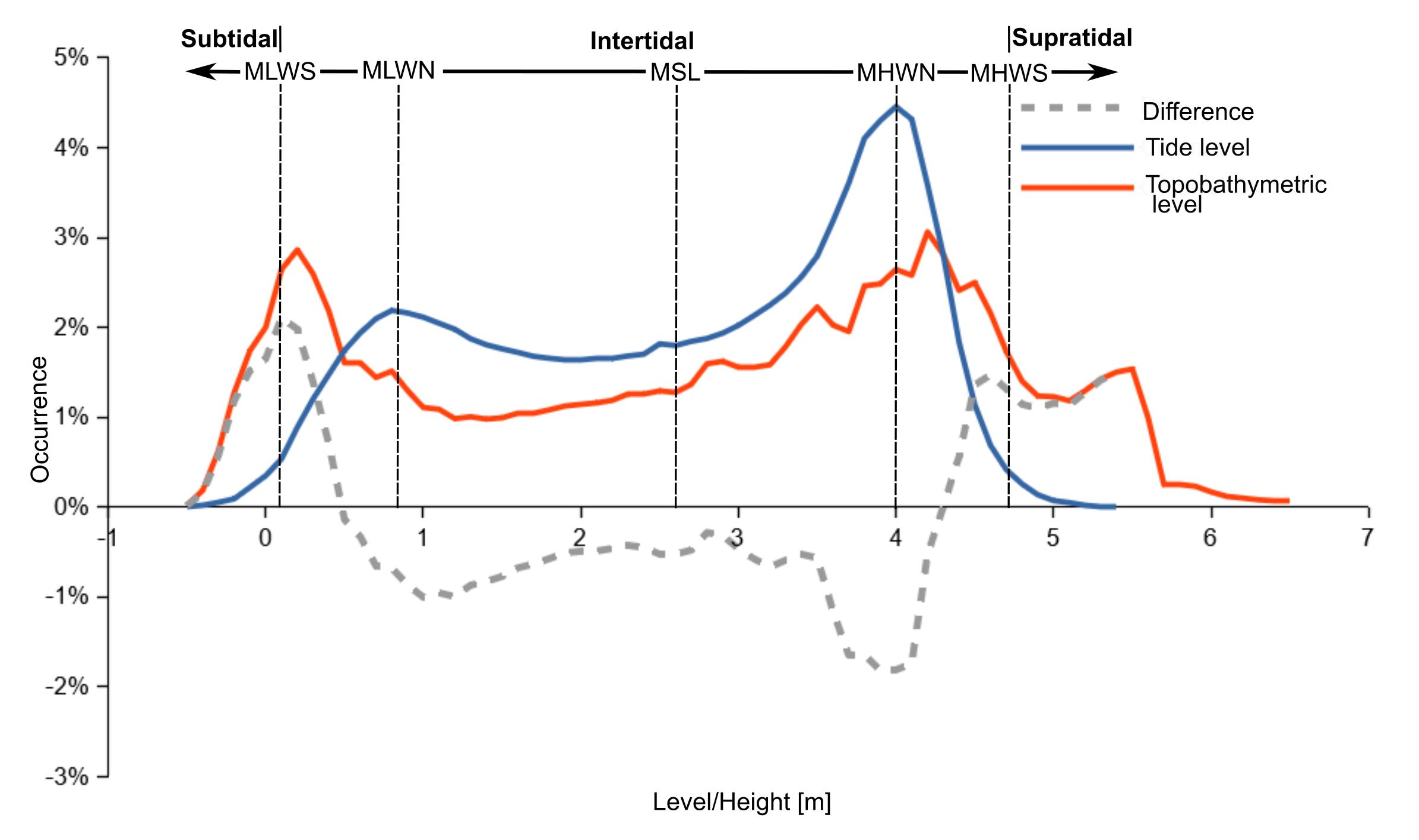
Figure 1.
Study area location map. Modified from Melo W.D., Instituto Argentino de Oceanografía.

Figure 2.
Flowchart showing the main stages of the proposed methodology. UAV: unmanned aerial vehicle; SfM: structure from motion; USV: unmanned surface vessel; GCP: ground control point; CP: checkpoint; PC: point cloud; BPC: Bathymetric point cloud; TPC: topographic point cloud.
Figure 2.
Flowchart showing the main stages of the proposed methodology. UAV: unmanned aerial vehicle; SfM: structure from motion; USV: unmanned surface vessel; GCP: ground control point; CP: checkpoint; PC: point cloud; BPC: Bathymetric point cloud; TPC: topographic point cloud.

Figure 3.
Equipment for topographic survey: (a) unmanned aerial vehicle (UAV); (b) flight path; (c) ground control points and checkpoints (left), and marker (18 cm diameter) (right); and (d) real-time kinematic (RTK) GPS base station (left) and rover (right).
Figure 3.
Equipment for topographic survey: (a) unmanned aerial vehicle (UAV); (b) flight path; (c) ground control points and checkpoints (left), and marker (18 cm diameter) (right); and (d) real-time kinematic (RTK) GPS base station (left) and rover (right).

Figure 4.
Equipment for bathymetric survey: (a) unmanned surface vessel (USV); (b) USV surveying the tidal channel; (c) zig-zag trajectory of the USV; and (d) parallel trajectory of the USV.
Figure 4.
Equipment for bathymetric survey: (a) unmanned surface vessel (USV); (b) USV surveying the tidal channel; (c) zig-zag trajectory of the USV; and (d) parallel trajectory of the USV.

Figure 5.
Structure from motion model: (a) map showing the number of overlapped images; (b) cleaned dense point cloud with 29 million points; and (c) orthomosaic.
Figure 5.
Structure from motion model: (a) map showing the number of overlapped images; (b) cleaned dense point cloud with 29 million points; and (c) orthomosaic.

Figure 6.
Accuracy assessment map of the bathymetry against the topography along random transects (T) and perimeter.
Figure 6.
Accuracy assessment map of the bathymetry against the topography along random transects (T) and perimeter.

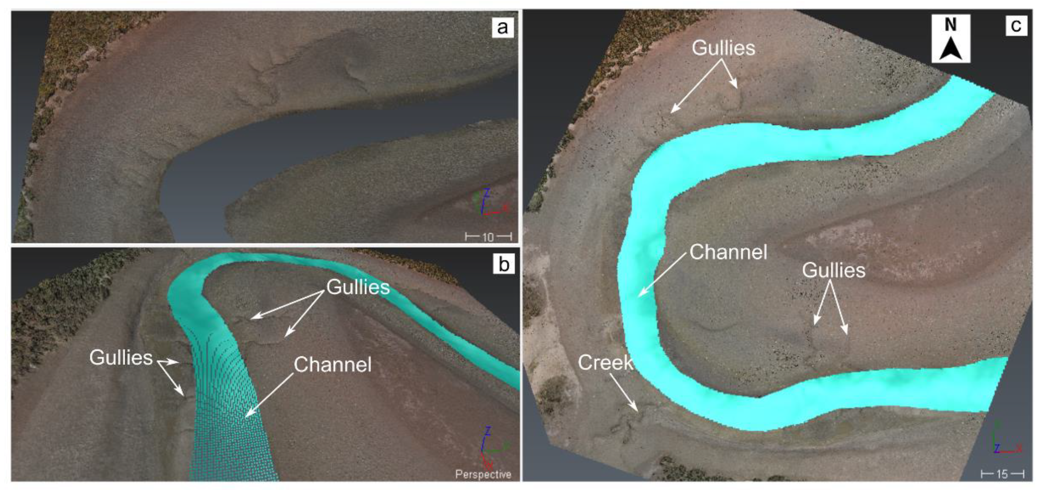
Figure 7.
Different views of the point clouds: (a) topographic point cloud; (b,c) topobathymetric point cloud showing the merging of two data sources and its main terrain features.
Figure 7.
Different views of the point clouds: (a) topographic point cloud; (b,c) topobathymetric point cloud showing the merging of two data sources and its main terrain features.

Figure 8.
Transverse topobathymetric profiles: (a) location map and (b) profiles including zoom views at the edges between TPC and BPC.
Figure 8.
Transverse topobathymetric profiles: (a) location map and (b) profiles including zoom views at the edges between TPC and BPC.

Figure 9.
Plot of the topobathymetric level and the tide level jointly with the main stage/conditions of the tide, allowing us to classify the study area into hydrogeomorphic zones (subtidal, intertidal, and supratidal).
Figure 9.
Plot of the topobathymetric level and the tide level jointly with the main stage/conditions of the tide, allowing us to classify the study area into hydrogeomorphic zones (subtidal, intertidal, and supratidal).

Figure 10.
Images of the topobathymetric model covered by the tide at different stages/conditions: (a) MLWS; (b) MLWN; (c) MSL; (d) MHWN; and (e) MHWS. MHWS/MLWS: high/low water spring; MHWN/MLWN: high/low water neap; MLS: mean sea level.
Figure 10.
Images of the topobathymetric model covered by the tide at different stages/conditions: (a) MLWS; (b) MLWN; (c) MSL; (d) MHWN; and (e) MHWS. MHWS/MLWS: high/low water spring; MHWN/MLWN: high/low water neap; MLS: mean sea level.


Table 1.
Technical specifications of the unmanned surface vessel (USV) (EMAC, USV v1.5).
| USV Specification | Description |
|---|---|
| Technical Specifications | |
| Cruising speed | 1.5 m s−1 |
| Vehicle weight | ≈12 kg (depending on battery configuration) |
| Payload weight | 4 kg |
| Maximum payload weight | 7 kg |
| Storage capacity | 5 L |
| Dimension | 1 × 0.45 × 0.27 m |
| Standard operation time | 6 h |
| Standard battery bank | 4S - 32,000 mA (2 batteries, 4S - 16,000 mA) |
| Extended battery bank | 4S - 64,000 mA (4 batteries, 4S - 16,000 mA) |
| Autopilot | Ardupilot 2.5 (stable-2.5.1/apm2) |
| Radio telemetry modem | RDF900, 900Mhz, 1W |
| Sonar option 1 | Garmin echo™ 100 (modified to capture the sonar signal; depth resolution: 0.1% FS) |
| Sonar option 2 | Bluerobotics - Ping Sonar |
| Working conditions | |
| Air temperature range | −10 to 50 Cº |
| Wind speed tolerance | Up to 14 m s−1 (calm waters) |
| Wave height tolerance | Up to 1 m |
| Minimum turning radius | 2.5 m |
| Water flow tolerance (opposite flow direction) | Up to 0.5 m s−1 |
| Water level depth | From 0.3 up to 100 m (depending on transducer) |
Table 2.
Ground control point (GCP) and checkpoint (CP) errors in the x, y, and z coordinates. All values are expressed in m. SD: standard deviation; MAV: mean absolute value; RMSE: root mean square error.
Table 2.
Ground control point (GCP) and checkpoint (CP) errors in the x, y, and z coordinates. All values are expressed in m. SD: standard deviation; MAV: mean absolute value; RMSE: root mean square error.
| GCP/CP | X | Y | Z |
|---|---|---|---|
| GCP1 | 0.239 | 0.206 | −0.094 |
| GCP2 | −0.0208 | 0.126 | 0.102 |
| GCP3 | −0.110 | −0.148 | −0.055 |
| GCP4 | 0.0139 | −0.184 | 0.005 |
| GCP5 | 0.0556 | −0.003 | 0.074 |
| GCP6 | 0.1095 | 0.0312 | −0.100 |
| GCP7 | −0.266 | −0.008 | 0.018 |
| Mean | 0.003 | 0.003 | −0.007 |
| SD | 0.161 | 0.139 | 0.079 |
| MAV | 0.116 | 0.101 | 0.064 |
| RMSE | 0.149 | 0.129 | 0.074 |
| CP1 | −0.130 | −0.036 | 0.106 |
| CP2 | −0.075 | 0.067 | 0.027 |
| CP3 | 0.126 | 0.015 | 0.096 |
| CP4 | −0.063 | −0.080 | −0.113 |
| Mean | −0.036 | −0.009 | 0.029 |
| SD | 0.112 | 0.064 | 0.101 |
| MAV | 0.099 | 0.049 | 0.086 |
| RMSE | 0.103 | 0.056 | 0.092 |
Table 3.
Accuracy of interpolated bathymetric datasets using different interpolation methods for each transect (T) and perimeter (P). All values are expressed in m. IDW: inverse distance weighting; K: kriging; NaN: natural neighbor; MC: minimum curvature; RMSE: root mean square error; MAE: mean absolute error; R2: coefficient of determination.
| Interp. Method | Error Analysis | T1 | T2 | T3 | T4 | T5 | T6 | T7 | T8 | P | Average |
|---|---|---|---|---|---|---|---|---|---|---|---|
| IDW25 | RMSE | 0.092 | 0.258 | 0.168 | 0.114 | 0.139 | 0.271 | 0.167 | 0.174 | 0.224 | 0.179 |
| MAE | −0.058 | 0.251 | 0.059 | −0.055 | −0.100 | 0.216 | 0.138 | 0.002 | 0.050 | 0.056 | |
| R2 | 0.900 | 0.926 | 0.569 | 0.960 | 0.979 | 0.946 | 0.986 | 0.992 | 0.921 | 0.909 | |
| IDW50 | RMSE | 0.099 | 0.238 | 0.195 | 0.099 | 0.164 | 0.258 | 0.158 | 0.153 | 0.213 | 0.175 |
| MAE | −0.068 | 0.211 | 0.087 | −0.048 | −0.119 | 0.202 | 0.129 | 0.043 | 0.046 | 0.054 | |
| R2 | 0.910 | 0.893 | 0.533 | 0.967 | 0.972 | 0.948 | 0.986 | 0.987 | 0.927 | 0.903 | |
| K25 | RMSE | 0.170 | 0.379 | 0.263 | 0.107 | 0.173 | 0.271 | 0.167 | 0.205 | 0.215 | 0.217 |
| MAE | 0.059 | 0.346 | 0.214 | 0.034 | −0.081 | 0.126 | 0.054 | 0.169 | 0.026 | 0.105 | |
| R2 | 0.640 | 0.838 | 0.795 | 0.948 | 0.915 | 0.896 | 0.958 | 0.973 | 0.917 | 0.876 | |
| K50 | RMSE | 0.163 | 0.369 | 0.235 | 0.118 | 0.165 | 0.251 | 0.129 | 0.209 | 0.221 | 0.207 |
| MAE | 0.013 | 0.329 | 0.189 | 0.023 | −0.077 | 0.093 | 0.045 | 0.169 | −0.005 | 0.087 | |
| R2 | 0.595 | 0.800 | 0.826 | 0.942 | 0.919 | 0.906 | 0.976 | 0.971 | 0.912 | 0.872 | |
| NaN25 | RMSE | 0.168 | 0.344 | 0.301 | 0.101 | 0.181 | 0.242 | 0.172 | 0.142 | 0.207 | 0.207 |
| MAE | 0.009 | 0.317 | 0.233 | 0.042 | −0.082 | 0.153 | 0.000 | 0.110 | 0.030 | 0.090 | |
| R2 | 0.680 | 0.902 | 0.714 | 0.945 | 0.916 | 0.937 | 0.952 | 0.985 | 0.923 | 0.884 | |
| NaN50 | RMSE | 0.196 | 0.360 | 0.257 | 0.121 | 0.162 | 0.203 | 0.119 | 0.205 | 0.215 | 0.204 |
| MAE | 0.027 | 0.328 | 0.221 | 0.059 | −0.037 | 0.112 | 0.016 | 0.171 | 0.010 | 0.101 | |
| R2 | 0.562 | 0.868 | 0.855 | 0.957 | 0.910 | 0.953 | 0.978 | 0.980 | 0.916 | 0.886 | |
| MC25 | RMSE | 0.211 | 0.396 | 0.296 | 0.118 | 0.206 | 0.278 | 0.186 | 0.329 | 0.237 | 0.251 |
| MAE | 0.046 | 0.365 | 0.245 | 0.050 | −0.088 | 0.107 | 0.045 | 0.269 | 0.028 | 0.118 | |
| R2 | 0.551 | 0.867 | 0.809 | 0.939 | 0.872 | 0.878 | 0.951 | 0.945 | 0.898 | 0.857 | |
| MC50 | RMSE | 0.225 | 0.400 | 0.278 | 0.116 | 0.194 | 0.254 | 0.144 | 0.311 | 0.243 | 0.241 |
| MAE | 0.045 | 0.358 | 0.230 | 0.044 | −0.086 | 0.067 | 0.032 | 0.244 | −0.003 | 0.103 | |
| R2 | 0.455 | 0.809 | 0.848 | 0.946 | 0.887 | 0.893 | 0.971 | 0.956 | 0.891 | 0.851 |
Table 4.
Costs and characteristics of the survey equipment used in the field study. WS: wind speed; WLD: water level depth.
Table 4.
Costs and characteristics of the survey equipment used in the field study. WS: wind speed; WLD: water level depth.
| Brand /Model | Price (US$) | Auto- Nomy | Survey Rate (km2 h−1) | Working Conditions | Operational Complexity | Post-pro- Cessing Complexity | Sample Point Density | Inva- Sivity | |
|---|---|---|---|---|---|---|---|---|---|
| UAV | DJI/Phantom 3 standard | 500 to 600 | 15 to 20 min | ≈0.16 (at 70 m height) | WS up to 7 m s−1; no rain; sunlight | Simple | Complex | High | Low |
| USV | EMAC/USV v1.5 | 800 to 1000 | 6 to 8 h | ≈0.06 | WS up to 10 m s−1; WLD from 0.3 m, waves heights less than 0.5 m | Medium | Simple | Medi-um | Low |
| RTKGPS | Swiftnav/Piksi RTK | 1000 | 4 to 24 h | - | Clear sky to party cloudy | Complex | Simple | Low | Mediumto high |
© 2020 by the authors. Licensee MDPI, Basel, Switzerland. This article is an open access article distributed under the terms and conditions of the Creative Commons Attribution (CC BY) license (http://creativecommons.org/licenses/by/4.0/).
Share and Cite
MDPI and ACS Style
Genchi, S.A.; Vitale, A.J.; Perillo, G.M.E.; Seitz, C.; Delrieux, C.A. Mapping Topobathymetry in a Shallow Tidal Environment Using Low-Cost Technology. Remote Sens. 2020, 12, 1394. https://0-doi-org.brum.beds.ac.uk/10.3390/rs12091394
AMA Style
Genchi SA, Vitale AJ, Perillo GME, Seitz C, Delrieux CA. Mapping Topobathymetry in a Shallow Tidal Environment Using Low-Cost Technology. Remote Sensing. 2020; 12(9):1394. https://0-doi-org.brum.beds.ac.uk/10.3390/rs12091394
Chicago/Turabian StyleGenchi, Sibila A., Alejandro J. Vitale, Gerardo M. E. Perillo, Carina Seitz, and Claudio A. Delrieux. 2020. "Mapping Topobathymetry in a Shallow Tidal Environment Using Low-Cost Technology" Remote Sensing 12, no. 9: 1394. https://0-doi-org.brum.beds.ac.uk/10.3390/rs12091394
Note that from the first issue of 2016, this journal uses article numbers instead of page numbers. See further details here.