1. Introduction
The increasing demand for food and bioenergy in the world stimulated the development of land suitability calculation methods, as a basis for effective agricultural land management and environmental sustainability [
1,
2]. Conventional agriculture is characterized by a very high input of fertilizer, pesticides and herbicides, having a negative long-term impact on sustainability [
3]. The selection of naturally suitable areas for the particular crop type cultivation reduces the overall application of inputs, creating an optimal environment for crop growth [
4]. Agricultural land management plans based on inappropriate evaluation of natural resources limit crop yields and increase production costs [
5]. Chen et al. [
6] recommended the development of crop-specific evaluation indices through land suitability determination to ensure the sustainability of agricultural production. Delineation of suitability classes with homogenous characteristics is a fundamental segment of land evaluation, allowing effective implementation of land use planning in the field [
7]. Mapping of such suitability classes for particular crop cultivation is essential for the transfer of knowledge to the end-users, whether to land management experts or individual farmers and farming companies [
8].
Multicriteria analysis is widely recognized as the method for the selection of the most suitable (optimal) location and its alternatives in various areas, such as agriculture [
9,
10,
11], forestry [
12], land management [
13] and environmental planning [
14]. With the integration of spatial components from Geographic Information System (GIS), an approach of GIS-based multicriteria analysis enables a suitability modeling for any entity related to space [
15]. The benefit of GIS-based multicriteria analysis in agriculture is its universal applicability regarding crop types, area size and location in the world. Its potential is conditioned only by the crop expert’s knowledge of the optimal agroecological conditions of the selected crop type and the quality of the input spatial data [
16,
17]. The core procedures of multicriteria analysis are based on the establishment of the relationship between relevant criteria [
18]. Many methods have been developed to determine the relative relationship between criteria for the suitability calculation, one of the most notable being the Analytic Hierarchy Process (AHP) [
19]. Standardization of criteria values is a necessary procedure in the calculation of suitability models [
20]. Input values of all criteria are commonly transformed into a unique number interval during the standardization process for further processing. Many authors noted an impact of the selection of standardization methods in multicriteria analysis on land suitability values [
21,
22,
23,
24]. Standardization using simple linear scale transformation was usually the selected method in these studies. The hybridization of GIS-based multicriteria analysis with unsupervised classification presents a novel approach in the management of calculated suitability values, enabling the effective creation of land suitability classes [
25]. The delineation of suitability classes is regarded as a necessary procedure in suitability analyses and precision agriculture, as it significantly facilitates the application of GIS-based multicriteria analysis results in the field [
26]. Van Niekerk noted the superiority of computer algorithms over traditional manual mapping techniques for the delineation of suitability classes, as they allow objective and time-efficient classification [
27].
Soybean is a fundamental component of agricultural land management plans worldwide, presenting a major source of protein for humans and a high-quality animal feed [
28]. According to the Food and Agriculture Organization of the United Nations (FAO) publication [
29], soybean accounted for about one-third of the total harvested area devoted to annual and perennial crops, while its share in global oil-crop output was 44%. According to the projection by the European Commission for the period between 2019 and 2030, the production of soybean food products will continue to grow due to demand for locally produced plant-protein food [
30]. The same source stated that the soybean area would show significant land-use change, resulting in a 5% harvested area increase by 2030. The long-term projection from the United States Department of Agriculture to 2029 predicts continuous global demand for soybean oil for biodiesel production [
31]. The competitive position of soybean among arable crops has steadily improved due to consistent improvements in yield and reductions in production costs [
29]. However, additional investment for soybean yield improving research was urged to land policymakers and managers [
32].
Medium-resolution multispectral satellite imagery presents an important data source for the observation of crop characteristics in yield improving research and mapping for agricultural land management [
33,
34]. Sentinel-2 is a multispectral satellite mission from the European Space Agency Copernicus program, started in 2015 [
35]. The constellation of Sentinel-2 mission is based on two satellites, Sentinel-2A (S2A) and Sentinel-2B (S2B), orbiting 180° apart [
36]. Sentinel-2 provides the possibility of an effective crop monitoring, having a 290 km swath width, high imaging resolution (up to 10 m) and revisit time of two to three days at mid-latitudes [
36]. Crop parameters with the application of remote sensing are commonly monitored using vegetation indices [
37]. The most used vegetation index is the Normalized Difference Vegetation Index (NDVI), which enables the determination of the relationship between photosynthetic and optical properties of crops [
38]. NDVI is the most widely used indicator in studies regarding crop biomass and chlorophyll content [
39]. Satellite-derived vegetation indices have been successfully used as a part of various crop models, such as the estimation of maximum evapotranspiration and irrigation requirements [
40] and multitemporal crop monitoring [
38].
The general objective of the study was the determination of optimal soybean land suitability and its mapping based on GIS-based multicriteria analysis. For this purpose, the evaluation of the three most commonly used standardization methods in recent GIS-based multicriteria analysis studies was conducted. The validation of calculated suitability values was performed using a novel peak NDVI method derived from Sentinel-2 multitemporal images as an independent accuracy assessment.
2. Materials and Methods
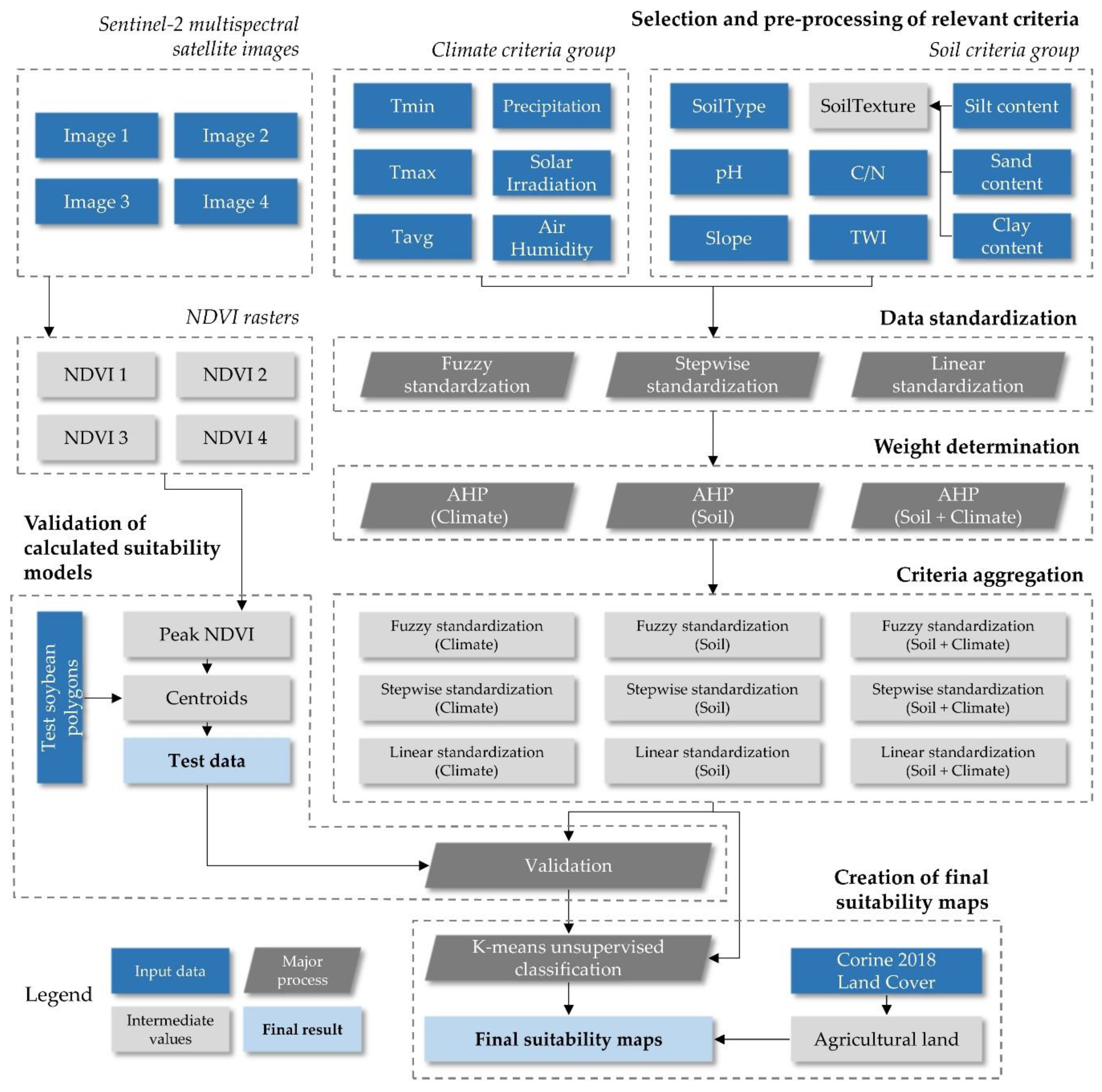
The proposed method of GIS-based multicriteria analysis for soybean suitability calculation and its validation consists of six major steps (
Figure 1). These are the selection and preprocessing of relevant criteria, data standardization, weight determination, criteria aggregation, validation of calculated suitability models and creation of final suitability maps. Open-source GIS software was used in this research: SAGA GIS v7.4.0 (Hamburg, Germany) [
41] for data preprocessing and calculations, QGIS v3.8.3 (Grüt, Switzerland) [
42] for data visualization and GRASS GIS v7.8.2 (Bonn, Germany) [
43] for the calculation of solar irradiation.
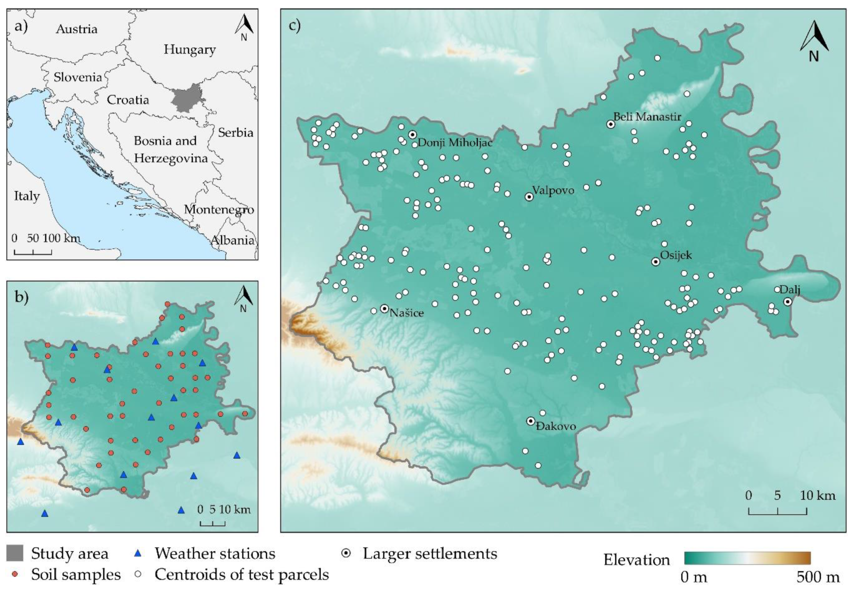
2.1. Study Area
The study area covers Osijek-Baranja County, a 4155 km
2 area located in eastern Croatia (
Figure 2). According to the Croatian Bureau of Statistics [
44], Osijek-Baranja County has the largest utilized agricultural area in Croatia, covering 13.6% of total country agricultural land in 2016. Corine 2018 Land Cover data showed that agricultural areas are the dominant land cover class in the county, covering 64.5% of the county’s area. Forests are the second-largest class covering 26.7% of the county’s area, followed by artificial surfaces (3.8%), wetlands (2.7%) and water bodies (2.3%). Croatia follows a world trend of an increase in soybean cultivation. According to [
45], a total of 111,316 t was produced in 2013 and 244,075 t in 2016, a 119% soybean production increase during four years. Soybean is the fourth highest cultivated crop in the study area behind maize, wheat and sunflower, covering 8.54% of the total agricultural land in the county during 2019 per Croatian Paying Agency for Agriculture, Fisheries and Rural Development data. Osijek-Baranja County has a moderately warm, rainy climate on a Köppen scale, according to the same source. Early soybean variants were commonly sown in eastern Croatia in recent years [
46]. Sowing of these variants was conducted in late April, while harvest typically occurred mid-October. The Croatian agricultural and forestry advisory service recommends the application of 30 kg/ha of nitrogen (N), 60 kg/ha of phosphorus pentoxide (P
2O
5) and 90 kg/ha of potassium oxide (K
2O) during basic fertilization in autumn and minor adjustments before sowing [
47]. Irrigation of soybean fields has been extremely overlooked in the study area, with only 64 ha employing some sort of irrigation system, according to Croatian Paying Agency for Agriculture, Fisheries and Rural Development data for 2019.
2.2. Selection and Preprocessing of Relevant Criteria
Climate and soil criteria were considered to have the most significant impact on soybean cultivation, based on previous research regarding soybean land suitability [
48,
49,
50,
51,
52]. Relevant climate and soil criteria selected in this study are shown in
Table 1. The selected number of criteria in each criteria group is six, which meets the specifications for the application of the AHP method for the consistency of information between criteria [
53]. The main data sources for the modeling of selected criteria were: Croatian Meteorological and Hydrological Service (DHMZ) data during the soybean growth period between April and October for years 2015–2019; Croatian Agency for the Environment and Nature (CAEN) soil samples collected during 2016; a basic pedologic map of Croatia; Shuttle Radar Topography Mission (SRTM) and Advanced Spaceborne Thermal Emission and Reflection Radiometer (ASTER) global digital elevation models.
Climate criteria consisting of T
min, T
avg, T
max, Precipitation and AirHumidity were interpolated from 15 DHMZ weather station data. Soil samples for modeling of soil criteria were downloaded from HAOP Web Feature Service. Samples were collected in the field by Croatian Geological Survey and Croatian Agency for Agricultural Land according to standards ISO 10390:2005 for soil pH, ISO 11277:2009 for soil texture and ISO 11466:1995 for soil C/N. From 72 regularly distributed samples in the study area, 48 were detected as agricultural area land cover and filtered for further processing. The solar irradiation criterion was defined as Global Horizontal Irradiation (GHI), according to previous research [
54]. GHI was calculated using the novel method developed by Gašparović et al. [
55], based on the ASTER digital elevation model, Linke turbidity factor [
56] and effective cloud albedo acquired from Meteosat Second Generation satellites SARAH Edition 2 [
57]. According to Gašparović et al. [
55], GHI produced 3% higher accuracy than commercial solar irradiation data, compared to the data measured from ground stations. The same approach for GHI calculation was successfully applied in similar research [
14]. The final GHI used in this research was an average daily mean value (kWh/m
2) between April and October in 2013 to 2015. A three-year period was used to reduce the influence of weather conditions. The time frame between April and October covers the vegetation period of all major soybean varieties cultivated in the study area. T
min represents a mean minimum air temperature for April and May, as soybean is most susceptible to frost at early vegetation stages that occur during April and May. T
max represents mean maximum air temperatures in June, July and August and refers to the drought risk. Soil type classes were derived from a basic pedologic map of Croatia. Soil pH was selected as a criterion due to soybean demands for neutral soil, with neutral and mildly acidic soils having optimal values. Soybean does not have strict demands regarding soil C/N [
58], but it has a major impact on sustainable planning of overall agricultural production in the study area. Soil C/N deficiency presents a major issue in the study area [
59], so crop types with larger demands for C/N would benefit more for being cultivated on soil with higher soil organic content. Soil texture classification was conducted in twelve classes from the soil texture triangle, according to silt, sand and clay soil content [
60]. Loam was considered as the most suitable soil texture, allowing the optimal root system development for soybean [
61]. The process of soil texture raster generation from silt, sand and clay soil content rasters was automatized using Python v3.7.4 (Wilmington, Delaware, United States of America) [
62]. The slope was determined using SRTM 1-arc second global digital elevation model. The slope is associated with the exploitation of air humidity in soybean cultivation, which is important for its development in reproductive growth stages. Terrain slope values were considered as hilly terrain restricts the adequate exploitation of agricultural machinery. Topographic wetness index (TWI) was calculated in SAGA GIS for the determination of specific catchment areas, representing the effect of inclined slopes on the soil water content [
63].
Preprocessing of input criteria consisted of the conversion of polygon vector criterion to a raster format, georeferencing of weather station data and conversion to point vector format, evaluation of interpolation methods for climate and soil points, interpolation of these values using the most accurate method and clipping of rasters to study area extents. The selected projection coordinate system was the Croatian Terrestrial Reference System (HTRS96/TM, EPSG: 3765) with 250 m spatial resolution (ground sample distance), so all rasters were reprojected and resampled accordingly. Interpolation methods selected for interpolation accuracy assessment were Ordinary Kriging (OK) [
64], Inverse Distance Weighting (IDW) [
65] and Angular Distance Weighting (ADW) [
66]. OK and IDW were selected as they resulted as the most accurate interpolation methods for the interpolation of soil parameters in studies by Yao et al. and Qiao et al. [
67,
68]. IDW and ADW produced the highest accuracy of tested deterministic interpolation methods for climate data in a study by Xavier et al. [
69]. Descriptive statistics (
Table 2) were calculated for the determination of input samples normality and stationarity with the aim of selection of optimal interpolation method [
70]. The mathematical model and fitting range for OK interpolation were selected on the highest possible fitting coefficient of determination to variogram. Both IDW and ADW were performed with a weight parameter of 2. Accuracy assessment was conducted based on cross-validation with the leave-one-out procedure, with the coefficient of determination (
R2), root-mean-square error (
RMSE) and normalized
RMSE (
NRMSE) as statistical indicators.
NRMSE was calculated by dividing
RMSE with a respective average of measured values from input climate or soil samples.
2.3. Data Standardization
Three standardization methods were evaluated in this research: linear standardization, stepwise standardization and fuzzy standardization. The defined number intervals for standardization were closed intervals containing values from zero to one (0.00, 1.00) or one to zero (1.00, 0.00), where 0.00 designates least favorable and 1.00 designates the most favorable impact on suitability values. The integration of qualitative and quantitative criteria values was conducted in this procedure. Values from the selected number interval during standardization were designated to either thematic classes in case of qualitative criteria or input numeric values for quantitative criteria, according to the level of suitability. Linear, stepwise and fuzzy standardization were applied to all selected criteria, except for the qualitative criteria SoilType and SoilTexture. For the two qualitative criteria, stepwise standardization was selected as a standardization method, being the only method that could operate with qualitative values. Consequentially, these values were used in combination with all three applied standardization methods for quantitative criteria.
The linear standardization method, based on linear scale transformation, is the most frequently used deterministic method for standardization in GIS-based multicriteria analysis [
71]. The deterministic nature of the method ensures completely objective standardization, with no crop expert’s impact on the standardization result. Linear standardization produced good results for the standardization of distances to infrastructure objects [
72] and climate data for crop suitability calculation [
73]. The calculation of linear standardization values was based on the score range procedure [
20].
Stepwise standardization is also a commonly used standardization method in GIS-based multicriteria analysis [
74]. It is based on the distinctive selection of the input values in number intervals defined by the crop expert for the standardization in new classes. An arbitrary value in the standardization interval has been assigned to each new class, allowing an extensive subjective crop expert’s impact on the result. Four to six classes were used for stepwise standardization, depending on the heterogeneity of input criteria values. Stepwise standardization was successfully applied for the standardization of soil chemical properties [
75] and climate criteria [
76].
Fuzzy standardization was based on the application of fuzzy membership functions. Similarly to stepwise standardization, fuzzy membership functions allowed extensive impact on the standardization result by the subjective crop expert. Three membership functions were used in this research: linear, S-shaped and J-shaped [
77]. Linear membership function (2) was a base for the calculation of S-shaped (3) and J-shaped (4) membership function values. Topographic indicators, such as slope, were successfully standardized using fuzzy membership functions [
78]. The same method was also applied for the standardization of soil criteria [
79] and the combination of soil and climate criteria [
80] in agriculture land suitability calculations. Membership function parameters were marked as
a and
d for the definition of support, alongside
b and
c for the definition of the core of the membership function [
81]. The variety of selected membership functions allowed the subjective crop expert’s impact on the intensity of ascending and descending of standardized values. Intermediate values between parameter values were gradually calculated, allowing the continuous representation of the criteria effect on suitability. Equations for the calculation of the standardized values using fuzzy membership functions were derived from Novák [
77].
2.4. Weight Determination
Weight determination was conducted using the AHP method in three approaches for climate criteria group, soil criteria group and combined criteria group consisting of both climate and soil criteria. Two pairwise comparison matrices were created to quantify criteria weights for climate and soil criteria, as a base of the AHP method [
82]. Individual weights per criteria group were calculated using separate pairwise comparison tables. Climate and soil criteria groups were considered as equally influential in suitability result. The primary motive of using three approaches was the estimation of criteria groups’ impact on the suitability result in the validation process. This procedure allowed the criteria modifications for further application, through the elimination of redundant criteria and the addition of new criteria. AHP is regarded as one of the most advantageous weight determination methods in the multicriteria analysis by Musakwa [
83], primarily due to being flexible, straightforward and comprehensive. It was successfully applied in GIS-based multicriteria analyses for crop cultivation suitability [
10,
84,
85], irrigation suitability [
76,
86] and environmental analyses [
14].
Each combination of two criteria per criteria group was evaluated in pairwise comparison matrices by assigning the preferred criteria value ranging from 1 (equal preference) to 9 (extreme preference) [
82]. The determined values were associated with preferred criteria in the pairwise comparison matrix, while the reciprocal value was assigned to the less-preferred criteria. The consistencies of pairwise comparisons per matrix were evaluated by Consistency Ratio (
CR) (1), using the Consistency Index (
CI) (2) and the Random Consistency Index (
RI) [
87]:
where
λ is the average value of consistency vector and
n is the number of parameters.
RI values were predefined by Saaty [
87], depending on the number of compared criteria in the pairwise comparison matrix. The acceptable value of
CR is 0.10, while higher values indicate that the revision and modification of the pairwise matrix should be conducted [
88].
2.5. Criteria Aggregation
The weighted linear combination was the selected method for criteria aggregation in the process of soybean suitability calculation. It is the most commonly used aggregation method in the GIS-based multicriteria analyses [
89]. The advantages of the selected method were simplicity and time-efficiency in the criteria aggregation, as well as the objective selection of the most suitable location and its alternatives, ranked by the suitability values [
90].
The nine suitability combinations of three standardization methods and three weight determination methods were calculated, resulting in nine suitability maps. Soybean suitability index (
SSI) was selected as soybean land suitability value, ranging from 0 to 1. According to Eastman [
20], the equation for
SSI calculation using weighted linear combination was (3):
where
wi denotes the weight of factor
i,
Xi denotes the standardized values of factor
i and
C denotes a Boolean layer of constraints.
2.6. Validation of Calculated Suitability Models
Calculated suitability values were validated by NDVI values derived from Sentinel-2 Level 2A images. No official database or reliable records about yield exist in Croatia, so NDVI was selected as a basis for validation. Since it was derived from Sentinel-2 images, nearly global applicability is ensured. Four images were downloaded, reprojected to HTRS96/TM and clipped to study area extents to cover the soybean seed filling growth stage (R6). This growth stage is associated with the highest total above-ground biomass during the soybean phenology cycle [
91]. NDVI derived from Sentinel-2 images produced a high correlation with biomass and chlorophyll content of crops in previous research [
92]. Soybean total above-ground biomass also resulted in a high correlation with yield [
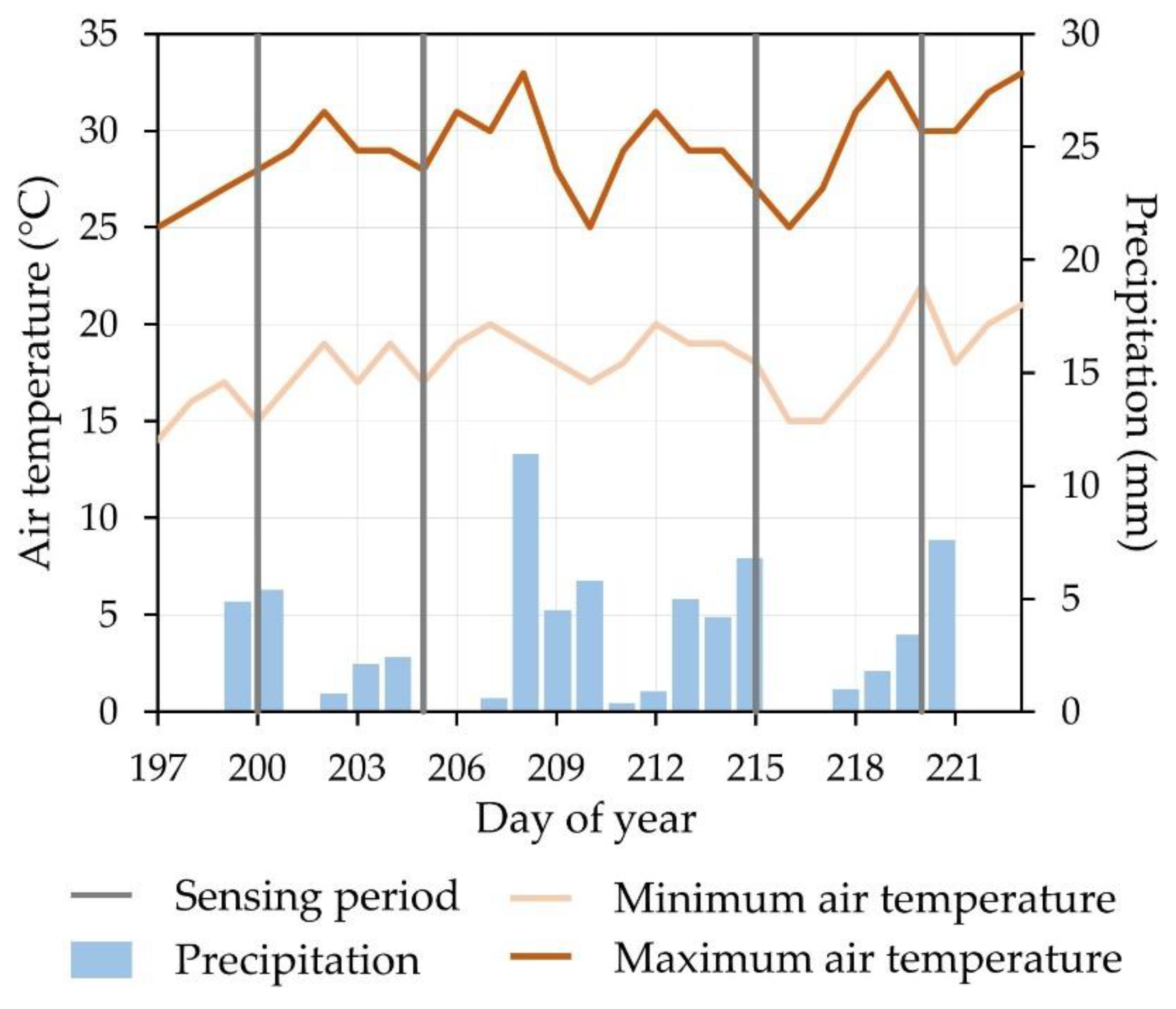
93]. These factors were selected as representative for validation with NDVI, as higher biomass and yield are expected on more suitable land for soybean cultivation. Not all soybean variants cultivated in the study area reach the R6 stage at the same time due to different periods of sowing, so the necessity for multitemporal images emerged. The time frame starting from 15 July to 10 August was determined for all soybean varieties in the study area to reach the R6 growth stage, based on the empirical knowledge of soybean cultivation in the study area. Four Sentinel-2 images were selected for validation from this time frame based on their availability and lowest possible cloud cover percentage (
Table 3). The used images were temporally evenly distributed in the time frame of the R6 soybean growth stage and sensed in very similar meteorological conditions (
Figure 3). All four NDVI images were used for the determination of peak NDVI of soybean test parcels, with slightly more than two-thirds having its peak NDVI during late July.
A total of 204 soybean test parcels, evenly distributed on the study area, were selected as the ground truth data. The total cumulative area of soybean parcels was 849.3 ha, with an average individual area of 4.16 ha. Shapefile vector data representing soybean parcels were collected from Croatian Paying Agency for Agriculture, Fisheries and Rural Development official spatial database, filtered by the soybean crop type. Four NDVI rasters derived from downloaded Sentinel-2 images were overlayed with the centroids of soybean parcels, so all NDVI values within a soybean parcel were averaged and designated to that centroid. Since spatial resolutions of suitability rasters and Sentinel-2 images were different (250 m and 10 m, respectively), centroids of reference soybean parcels with peak NDVI values were used to perform validation of suitability rasters. Centroids of soybean test parcels were forced inside polygons during creation to represent geometrically irregular parcels accurately. The comparison of these data sets was achieved with fast processing time, as point vector was overlayed with raster data. Peak NDVI values per centroid were determined as the maximum NDVI value per centroid, based on four NDVI rasters derived from multitemporal Sentinel-2 images.
The use of peak NDVI allowed the detection of the R6 growth stage for all ground truth polygons, which represented all soybean variants in the study area. Such a procedure proved to be robust regarding the atmospheric effects like clouds and haze on satellite images since validation does not depend on the individual images. Identification data of Sentinel-2 images used for the validation of suitability models are shown in
Table 2.
Four regression functions were selected for the calculation of R
2 between suitability values and reference peak NDVI values. Selected functions were linear (R
2lin), logarithmic (R
2log), exponential (R
2exp), second-order polynomial (R
2poly2) and third-order polynomial (R
2poly3). Different regression functions were evaluated to determine the most accurate relationship model between suitability values and peak NDVI. Validation of each suitability model was based on the highest R
2 calculated using these functions. RMSE and Cohen’s d index were calculated as a complementary statistical values to R
2 for accuracy assessment. Cohen’s d values were interpreted according to [
94]. Peak NDVI and suitability values were normalized in the (0.00, 1.00) range prior to RMSE and Cohen’s d calculation to describe suitability results while referring to the same number interval.
2.7. Creation of Final Suitability Maps
Unsupervised classification using the k-means algorithm was applied for the delineation of five suitability classes for each calculated suitability model. Created suitability classes were classified according to FAO standards in classes representing very suitable (S1), moderately suitable (S2), marginally suitable (S3), currently unsuitable (N1) and permanently unsuitable area (N2) [
95]. Unsupervised classification was therefore conducted in five classes to meet the FAO specification. Ranking of class suitability values was conducted using mean suitability values of all pixels per class. The selected method approached the suitability values on a relative basis using a computer-automated classification. This procedure enabled the creation of suitability classes independently of selected criteria or study area properties. Such an approach reduced the effect of subjectivity in the pairwise comparisons of criteria in AHP, which is its major disadvantage [
96]. For the application of this method in the regionalization of agricultural production, the integration of suitability values for different crop types, and consequentially from different crop experts, is necessary. By managing the suitability values using unsupervised classification, the integration was possible since the relative criteria relationship was retained. The crop experts’ judgment levels have been balanced in the process, preventing overestimation or underestimation of suitability. The applied approach also ensured the objectiveness in the creation of suitability classes, as the training data creation was not necessary, in contrast to supervised classification. Training data creation presents a common source of human error in classification due to the operator’s subjectivity in the selection of training polygons [
97]. Input data in the k-means algorithm was raster representing suitability values from the most accurate suitability model. Algorithms based on unsupervised classification were successfully applied for suitability classification with a single raster input [
27]. K-means was successfully applied in various combinations with GIS-based multicriteria analysis in crop suitability analyses [
25,
98,
99] and delineation of suitability classes in precision agriculture [
100]. Final suitability maps were created by the removal of constrained areas from the unsupervised classification results. CORINE 2018 Land Cover data was applied to exclude agricultural land cover, as no other land cover was available for efficient soybean cultivation. The goal of this step was to exclude permanent natural (forests, wetlands, water bodies) and built-up objects from classification in a 250 m spatial resolution, so CORINE 2018 Land Cover data was selected as the most fitting data source due to its high thematic accuracy (85%) [
101]. All calculated suitability models were mutually compared using Pearson’s correlation coefficient in the correlation matrix.
3. Results
The descriptive statistics of input samples for evaluation of interpolation methods are shown in
Table 3. Moderate skewness and high kurtosis deviations were observed from optimal values of zero and three, respectively. While low coefficients of variation indicated high data stationarity, low data normality was observed for both climate and soil criteria. Sand soil content was the only exception from this observation, as it produced both low normality and stationarity.
Accuracy assessment results of tested interpolation methods are shown in
Table 4. Both deterministic methods outperformed OK in a case of climate data with a lower number of samples. IDW was selected as an optimal method for the interpolation of climate data, producing higher accuracy values than ADW for T
min, Precipitation and AirHumidity. Accuracy of interpolation for T
avg and T
max produced mixed results, as ADW produced higher
R2 for T
avg and higher
RMSE and
NRMSE for T
max than IDW, but lower
RMSE,
NRMSE and
R2, respectively. All tested methods produced lower mean accuracy for soil data compared to climate data. IDW produced the highest accuracy values for the interpolation of moderately variable data: Clay, Silt and C/N. ADW produced the highest
R2 for pH interpolation and second-best
RMSE and
NRMSE values behind IDW. OK produced slightly higher
RMSE and
NRMSE for interpolation of sand, but 0.0346 lower
R2 than IDW. IDW was therefore also selected as an optimal interpolation method for soil data.
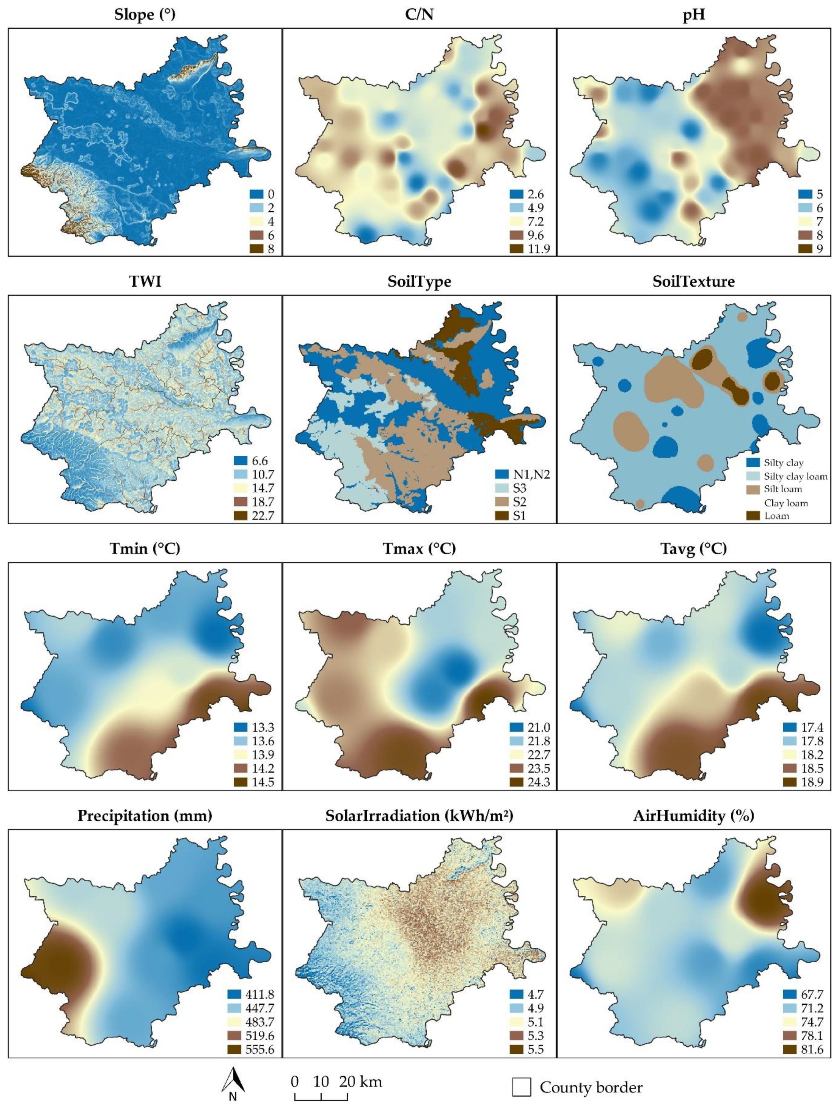
Soil texture classes resulting after classification were silty clay, silty clay loam, clay loam, loam and silt loam. The dominant soil texture class in the study area was silty clay loam, covering 72.1% of the total area. The next two largest classes, silty clay and silt loam, had significant silt content, covering 21.6% of the study area combined. Clay loam and loam mostly covered the transitional areas between two larger classes, resulting in 3.2% and 3.1% of the study area, respectively. All preprocessed input criteria rasters are shown in
Figure 4.
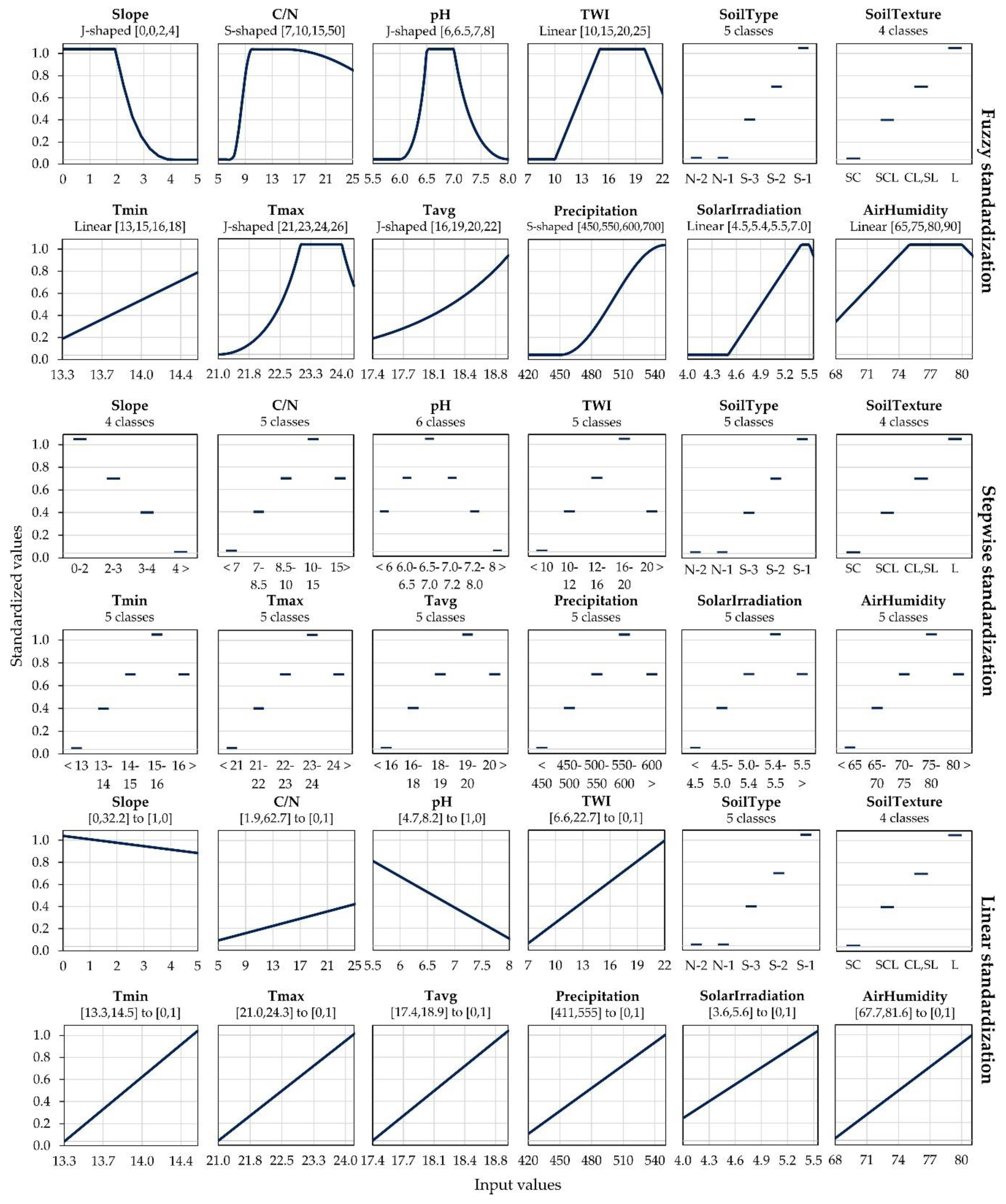
Parameters for each standardization method were selected as shown in
Figure 5. The presence of a few extreme input values prevented the linear standardization method to expand the full (0.00, 1.00) number interval to the majority of pixels, resulting in an inaccurate representation of these criteria. This primarily refers to slope and C/N, where the number interval covers most of the pixels in (0.85, 1.00) and (0.00, 0.25) number interval, respectively. Intermediate values for stepwise standardization were selected based on standardization classes count, alongside a minimum value of 0.00 and a maximum of 1.00. The J-shaped and linear methods were the most commonly used fuzzy membership function for standardization, both being applied for 4 out of 10 quantitative criteria. Precipitation, SolarIrradiation and AirHumidity resulted in a high variability, while T
avg, T
min and T
max produced moderate variability of the climate conditions in the study area. All soil criteria resulted in high variability in the study area.
Pairwise comparison matrices were created for climate (
Table 5) and soil criteria (
Table 6). Consistency tests for both matrices resulted in the allowed tolerance. The weight sums of interpolated criteria were 0.877 for climate and 0.431 for soil criteria group.
Calculated
R2, RMSE and Cohen’s
d values for the validation of suitability models are displayed in
Table 7. Suitability calculated using the climate criteria group constantly produced the lowest
R2, with a maximum for fuzzy standardization using exponential regression. Stepwise and fuzzy standardization models both produced the highest accuracies for soil and combined criteria groups, with combined variants being slightly more accurate. Overall, fuzzy standardization with combined criteria produced the highest
R2 and
RMSE, presenting the optimal model for soybean land suitability mapping.
RMSE values were based on normalized values, so they resulted in (0.00, 1.00) number interval and therefore enabled objective accuracy assessment of suitability values. Cohen’s
d values indicated the strongest relationship between fuzzy standardization and soil criteria with peak NDVI values. The fuzzy standardization with combined criteria also resulted in a small effect size, having a large value gap between the third-lowest
d value of fuzzy standardization with climate criteria.
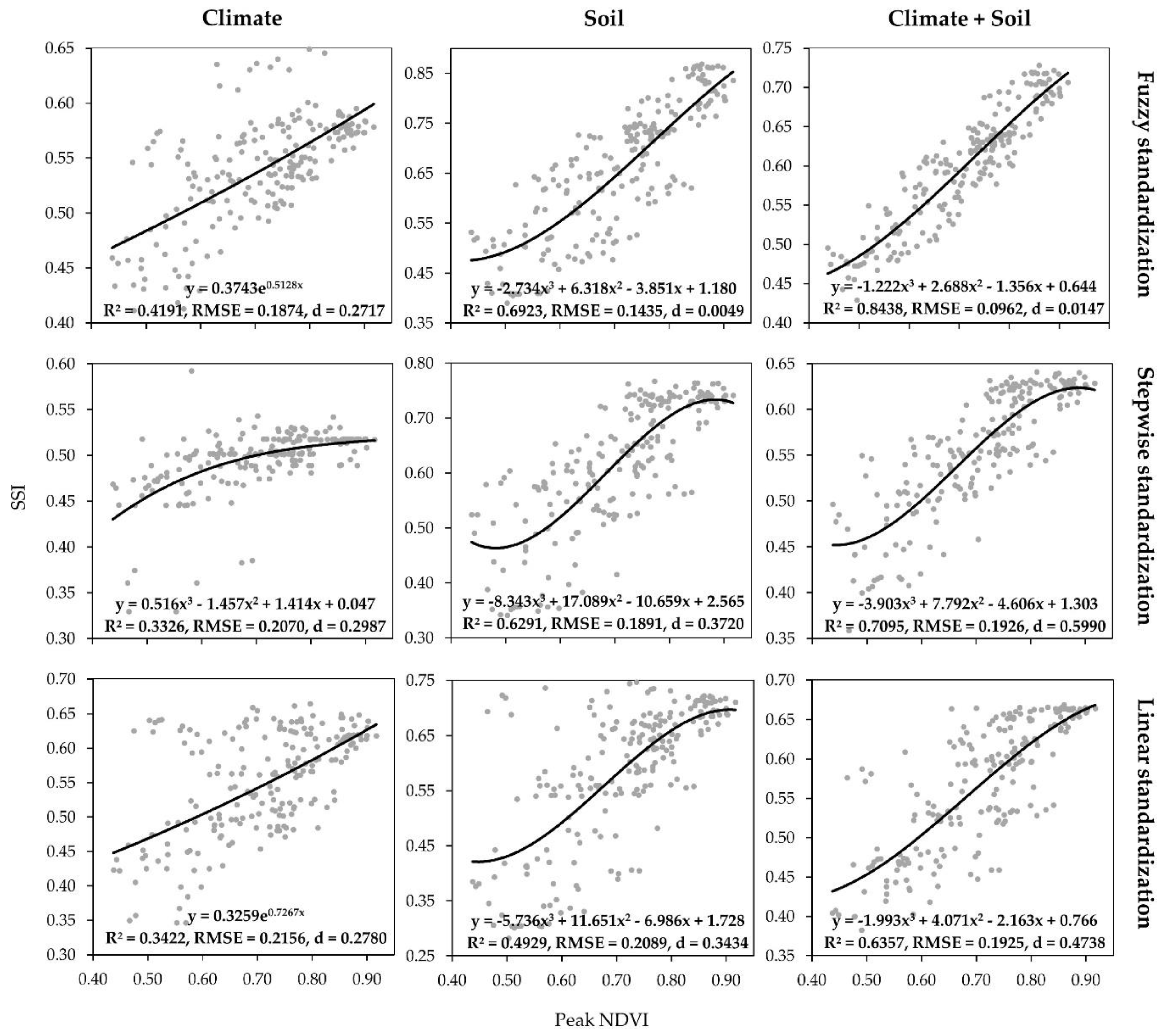
Visual representation of regression functions that produced the highest coefficient of determination per model is presented in
Figure 6. The similarity of stepwise and fuzzy standardization with soil and combined criteria results can be observed, with fuzzy models resulting in slightly smaller dispersion.
RMSE values showed similar results, as fuzzy methods produced lower
RMSE than stepwise standardization for both soil (difference 0.0456) and combined criteria group (difference 0.0964). Climate criteria resulted in the lowest sensitivity to the selected standardization method, having closely distributed values for all applied standardization methods. The third-order polynomial regression function resulted in the highest
R2 in the validation of all soil and combined criteria. The exponential function most accurately represented the relationship of suitability and peak NDVI values for climate criteria with fuzzy and linear standardization methods.
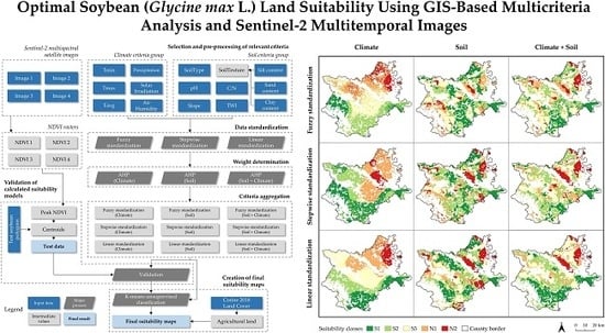
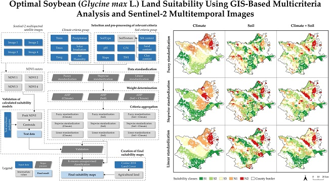
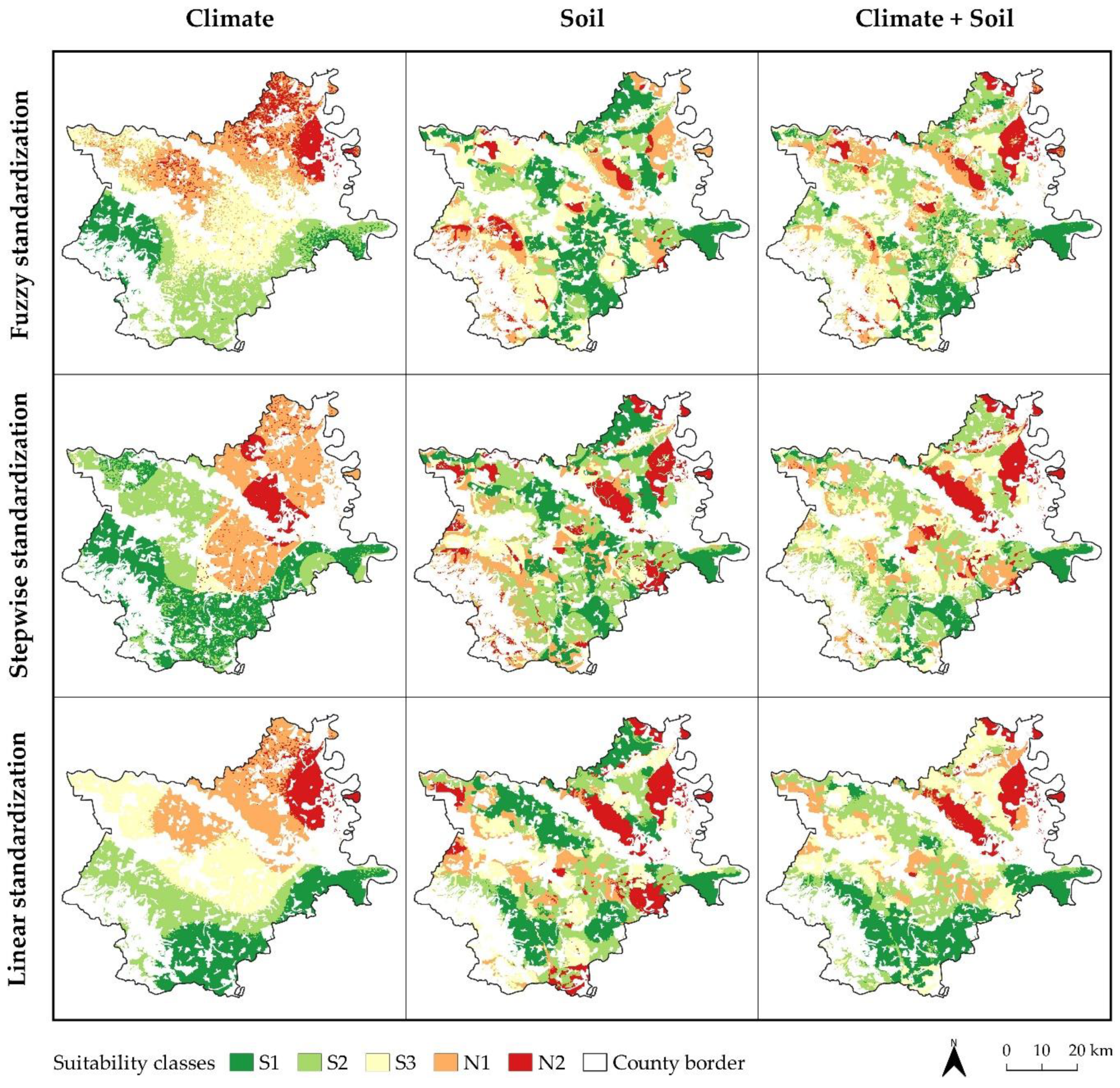
Shares of suitability classes calculated using k-means unsupervised classification regarding the covered area are shown in
Table 8. According to the most accurate suitability values calculated using fuzzy standardization and combined criteria, 64.3% of the study area is suitable for soybean cultivation to some degree. The S1 class covers 602 km
2 of the county area. The area determined as very suitable covers three major parts: the eastern part near Dalj, mainly characterized with high average minimal air temperatures; the northeastern part by the Baranja hill with optimal C/N values, pH and SoilType values; and the central-south part by the city of Đakovo with suitable SoilTexture and SoilType values. The final suitability maps after the removal of constrained areas from the unsupervised classification results are shown in
Figure 7. The most accurate suitability model was exported to vector Shapefile and raster GeoTIFF format.
Suitability classes: very suitable (S1), moderately suitable (S2), marginally suitable (S3), currently unsuitable (N1) and permanently unsuitable (N2).
The correlation matrix of all combinations of calculated suitability models (
Table 9) showed a constantly high correlation of suitability values calculated using soil and combined criteria for all three standardization methods. Suitability values using climate criteria produced a moderate correlation with combined criteria values. A high correlation was achieved for fuzzy and stepwise standardization with combined criteria, which produced two most accurate suitability values.
4. Discussion
Linear standardization was proven to be less effective in adjusting to standardization specifications for nearly all quantitative criteria. This occurred due to the linear standardization’s property of monotonous ascending or descending of standardized values in the specified number interval. Therefore, nonlinear varying standardization requirements of Precipitation, SolarIrradiation, T
avg, T
max, AirHumidity, pH and TWI could not be fully adjusted. However, linear standardization performed as the second-best standardization method for climate criteria, as few extreme values were present in these criteria. Stepwise standardization allowed high subjective impact on standardized results due to the ability to join the arbitrary input value ranges to standardization classes. These classes were discretely defined, with no intermediate values between classes. The most important property of the stepwise standardization method was the ability of the standardization of qualitative criteria, which presents a necessity for the integration with quantitative criteria. Fuzzy standardization methods allowed the best adjustment of standardized values to the crop expert’s specifications for quantitative criteria, consequentially resulting in the highest accuracies of suitability models. Aside from setting the intervals of least and most favorable input values, the crop expert also had supervision over the intensity of increasing and decreasing the standardized values by selecting the optimal fuzzy model. Sigmoidal and J-shaped membership functions were also recognized as the most convenient for the standardization of similar criteria in a study by Aydi et al. [
89]. Investigated properties of fuzzy standardization proved that it could be used as a universal standardization method, possibly upgrading the calculation of suitability values where linear and stepwise standardization were previously combined [
74]. The FAO guidelines offered a standard for the delineation of suitability classes, which enables a comparison between similar suitability models. These standards were applied in many studies regarding suitability analyses recently [
10,
15,
78]. The creation of suitability classes is considered as a necessary procedure in effective land management in similar studies. They were previously used in suitability analyses regarding crop cultivation and irrigation [
99].
Suitability models calculated with the combined criteria group produced the highest accuracy, showing the importance of climate and soil criteria groups in crop-related suitability analysis. A low correlation between models using only climate and soil criteria was observed for all standardization methods. Climate and soil criteria groups were both necessary for reliable suitability calculation [
7,
102]. The possible reason for the lower accuracy of suitability models that used climate criteria compared to soil or combined criteria is a relatively small study area (4,155 km
2), causing low variability for selected climate criteria. Precipitation produced the highest variability of all data from weather stations, with a CV of only 0.100. However, climate data was considered as mandatory criteria group especially in the case of the larger study area, having an impact on high suitability values for combined criteria. Many recent studies successfully integrated GIS-based multicriteria analysis with AHP as a weight determination method for crop suitability calculation [
11,
25,
80,
83,
84]. Besides weight determination, three modifications of AHP in this study enabled the determination of the reliability of input data used for the modeling of criteria per criteria groups. The combined criteria group produced the highest accuracy for all standardization methods. Fuzzy and stepwise standardization methods also produced moderate accuracy using soil criteria, while climate criteria produced the lowest accuracy. Linear standardization produced similar accuracies for all AHP modifications. Fuzzy standardization resulted in higher accuracy using the combined criteria group than the other two methods, due to better adjustment of values to the crop expert’s specifications in the standardization process. All interpolation methods performed better in case of less variable climate data compared to soil data. OK usually outperformed IDW in studies comparing interpolation methods for soil and climate data but has some limitations regarding normality and stationarity of input samples [
103]. IDW outperformed OK in case of low normality and high variability of sample data [
104]. Kriging was unable to produce quality results in when its prerequisites of sample data normality and stationarity were not met in a different study, where IDW resulted in higher accuracy [
25]. This emphasizes the importance of the selection of optimal interpolation method in similar studies as it depends on the properties of input samples [
105].
No standard methodology of crop suitability values validation calculated by GIS-based multicriteria analysis was noted during the literature review. Moreover, the majority of these studies did not employ any validation procedure for crop suitability results [
11,
25,
51,
83,
84,
89]. Multitemporal NDVI offers a potential solution in the validation of crop suitability, due to its global accessibility from global multispectral satellite missions (Sentinel-2, Landsat 8) and being a reliable predictor of various crop properties [
92]. Moreover, Sentinel-2 derived NDVI was a reliable predictor in a study of crop yield and was superior to other individual tested vegetation indices [
106]. The applicability of NDVI was expanded in this study as it enabled an effective validation of suitability models, primarily due to the objective assessment of all major soybean varieties using peak NDVI values. An application of NDVI in the validation of wheat suitability combined with yield data was successfully made in a study by Dedeoğlu and Dengiz [
107]. However, the application of peak NDVI values that were used for direct validation of suitability values before their classification in suitability classes represents a significant improvement for its applicability in suitability validation. Data about conducted agrotechnical operations (sowing, fertilization, spraying) for every test soybean parcel remain an ambiguity and could affect the reliability of validation using peak NDVI. Fertilization is traditionally balanced in the entire study area, but its exact effect on NDVI values for validation remain to be tested. Soybean satisfies around 60% of its nitrogen requirements by nitrogen fixation [
108], which is one of the reasons for farmers in the study area to apply conventional fertilization without conducting detailed soil analysis commonly. Therefore, nitrogen fertilization was not expected to have a significant impact during validation using NDVI. The effect of pests, diseases and weather trend on crop status prevent NDVI from being fully reliable validation data, as vegetation depends on numerous individual factors [
109]. A relatively small study area partially reduced the effects of weather conditions, having low variability. The averaging of NDVI values from soybean parcels to centroids allowed the lower impact of potentially affected areas by pests or disease. A possible solution for the mentioned restrictions is the integration of multiple complementary vegetation indices for validation, as the spectral resolution of Sentinel-2 allows for the calculation of most known vegetation indices [
110]. The Soil-Adjusted Vegetation Index (SAVI) is considered as one of the complementary indices to NDVI, as it minimized the soil brightness effect in areas with sparser vegetation in a comparable study [
111]. Of the four Sentinel-2 images used for the calculation of peak NDVI, the dataset sensed on 8 August 2019 produced the lowest amount of peak NDVI values due to the lack of precipitation at the beginning of the month. This case implies the importance of considering meteorological conditions for adjustment of the time frame for validation. The validation time frames should be slightly calibrated for each growing season, as drought could accelerate the ripening process of soybean, therefore lowering the vegetation indices values.
While the simplicity and effectiveness of the weighted linear combination for criteria aggregation were previously mentioned and successfully applied, the Ordered Weighted Averaging (OWA) method offers a potential upgrade to the applied methods. Its potential in GIS-based multicriteria analysis is primarily notable through the integration of fuzzy measures in the criteria aggregation process [
112]. OWA was successfully applied for suitability analysis of crops in combination with AHP [
113] and multicriteria analysis regarding soil chemical properties in combination with IDW as the interpolation method [
114]. The majority of applied methods for GIS-based multicriteria analysis in this study support the automatization of the calculation process, which will be a subject of future research. Inputs consisting of criteria selection, pairwise matrix comparison and standardization specifications should be assigned at the beginning of the algorithm. The main benefits of automatization in this research were noticeable during the process of soil texture map calculation, which are time-efficiency and easier applicability of the process to future calculations [
78]. Automatization is considered as a major property for making the GIS-based methods and algorithms considerably more applicable in regular practice [
115]. Since the user does not have to conduct each process in the GIS environment manually, the accessibility of automated methods expands to users with limited knowledge of geospatial data.
The addition of the ecological criteria group to the multicriteria analysis presents a possibility for the improvement of the present study. Aside from the ecological criteria group, the proposed method supports the addition of multiple other criteria groups through the creation of additional pairwise comparison matrices, as long as the number of criteria per group satisfies specifications by Saaty and Ozdemir [
53].


