Evaluating Downscaling Factors of Microwave Satellite Soil Moisture Based on Machine Learning Method


College of Geoscience and Surveying Engineering, China University of Mining and Technology-Beijing, Beijing 100083, China
*
Author to whom correspondence should be addressed.
Remote Sens. 2021, 13(1), 133; https://0-doi-org.brum.beds.ac.uk/10.3390/rs13010133
Submission received: 27 November 2020
/
Revised: 27 December 2020
/
Accepted: 29 December 2020
/
Published: 2 January 2021
Abstract
:Downscaling microwave remotely sensed soil moisture (SM) is an effective way to obtain spatial continuous SM with fine resolution for hydrological and agricultural applications on a regional scale. Downscaling factors and functions are two basic components of SM downscaling where the former is particularly important in the era of big data. Based on machine learning method, this study evaluated Land Surface Temperature (LST), Land surface Evaporative Efficiency (LEE), and geographical factors from Moderate Resolution Imaging Spectroradiometer (MODIS) products for downscaling SMAP (Soil Moisture Active and Passive) SM products. This study spans from 2015 to the end of 2018 and locates in the central United States. Original SMAP SM and in-situ SM at sparse networks and core validation sites were used as reference. Experiment results indicated that (1) LEE presented comparative performance with LST as downscaling factors; (2) adding geographical factors can significantly improve the performance of SM downscaling; (3) integrating LST, LEE, and geographical factors got the best performance; (4) using Z-score normalization or hyperbolic-tangent normalization methods did not change the above conclusions, neither did using support vector regression nor feed forward neural network methods. This study demonstrates the possibility of LEE as an alternative of LST for downscaling SM when there is no available LST due to cloud contamination. It also provides experimental evidence for adding geographical factors in the downscaling process.
1. Introduction
Water in the soil, especially the capillary one, is the chief water that is available to plants. Correspondingly, plants rely on water to facilitate photosynthesis, transfer nutrients, stimulate germination, and complete transpiration. Therefore, soil moisture (SM) is a critical factor that affects crop growth and food production [1]. Moreover, it is an essential land state variable that controls several water-cycle fluxes such as evapotranspiration (ET), penetration, and runoff. Obtaining spatial continuous SM data with fine spatiotemporal resolution has always been the demand in agricultural production [1], drought monitoring [2,3,4], water resource management [5], and climate change [6].
Remote sensing is an advanced measurement technology which has become a significant way to obtain spatially distributed SM from a regional to global scale [7,8,9]. Although various remote sensing methods have been explored to retrieve SM, such as the methods based on visible, near infrared, and thermal infrared bands, the microwave band-based methods (especially the L-band) have been recognized as the most promising techniques for global-scale monitoring [10]. That is because L-band microwave can penetrate clouds, sparse vegetation, and even the skin surface of soil which presents great potential for retrieving soil moisture over a much higher range of vegetation conditions [11]. However, the SM retrieved by microwave band-based methods generally has coarse spatial resolution at about a few tens of kilometers, which is not qualified to meet practical requirement for many hydrological and agricultural applications on a regional scale [12,13]. Thus, downscaling microwave satellite SM with multi-source remote sensing data has become a very meaningful research field [14].
Generally, there are two basic components in the algorithms of downscaling microwave satellite SM. They are downscaling factors and downscaling functions. The downscaling factors provide the spatial variability of high-resolution SM within the coarse-resolution SM. The downscaling functions determine the way of adding the spatial variability to the coarse-resolution SM [15]. Currently, three categories of downscaling functions exist in the study community i.e., physical model, parameterized model, and statistical regression model. Disaggregation based on Physical And Theoretical scale Change (DISPATCH) is a representative of the physical model [16,17]. Such a physical model generally runs on the quantitative relationship between SM and Soil Evaporative Efficiency (SEE). However, some parameters of the SM-SEE relationship are hard to be determined [17,18]. Besides, the real relationship between SM and SEE is very complex and the modeling techniques are still evolving [19]. Through making some necessary assumptions, parameterized models were proposed to achieve a tradeoff between efficiency and accuracy. For example, the relative ratio methods (UCLA) use a linear relationship to connect soil wetness index (SW) with soil moisture. In simple terms, the ratio of high-resolution SM to high-resolution SW is equal to the ratio of coarse-resolution SM to coarse-resolution SW [20]. Additionally, the change detection algorithm and its subsequent versions assume the SM and co-polarized backscatter are linearly related [21]. Based on this assumption, high-resolution SM can be expressed as the sum of coarse-resolution SM and spatial anomaly of high-resolution SM [11]. Recently, a new downscaling model DSCALE_mod16 was proposed. In this model, parameterized cosine expression of the relationship between SM and Land surface Evaporative Efficiency (LEE) was employed [22]. Although the parameterized models have been widely used, the key assumptions may have greater uncertainties for certain cases. For instance, the linear relationship assumption between SM and co-polarized backscatter may lose efficiency for high surface roughness and vegetation coverage [23]. Entering the era of big data and Artificial Intelligence (AI), the complex relationship between SM and various downscaling factors may be established by the statistical regression model [24]. Actually, the development of statistical regression has been accompanied by advances in computer science. Initially, polynomial fitting such as binary quadratic equation was used for downscaling SM [13,15,25]. Recently, being a subcategory of AI, various machine learning (ML) algorithms were proposed for downscaling SM such as General Regression Neural Network, Artificial Neural Network (ANN), Random Forest (RF), and Support Vector Regression (SVR) [26,27,28,29]. Through the above researches, the flexibility and capability of ML to deal with massive remote sensing data and nonlinear problems in downscaling SM have been proved [26]. This context highlights the importance of selecting proper downscaling factors in order to train the ML algorithms.
In classical optical/thermal and microwave fusion methods, Land Surface Temperature (LST) and Normalized Difference Vegetation Index (NDVI) were employed as downscaling factors with the understanding of the LST and Fractional Vegetation Coverage or vegetation index feature space (LST/FVC space) [15]. However, the LST/FVC space may lose efficiency in energy limited evapotranspiration regime [13]. Therefore, as the representativeness of energy portion, the surface net incoming radiation (Rn) or surface albedo is added as downscaling factors [13]. Furthermore, LST derived soil moisture indicators (SMIs) are also utilized as downscaling factors such as Vegetation Temperature Condition Index (VTCI) or Temperature Vegetation Dryness Index (TVDI) [30,31]. It has been recognized that the LST and LST-derived SMIs are vital to the optical/thermal and microwave fusion methods for disaggregating microwave satellite SM. However, the LST-related downscaling factors suffer the “cloud contamination,” “decomposing uncertainty,” and “decoupling effect” problems, which often make no available LST data for downscaling [22,26]. Recently, a new downscaling factor, i.e., Land surface Evaporative Efficiency (LEE), has been introduced [22]. The LEE is defined as the ratio of actual ET or latent heat flux (LE) to potential ET (PET) or potential LE (PLE) which were both obtained from the MODIS (Moderate Resolution Imaging Spectroradiometer) ET product (MOD16). Since LST is not involved in the calculation of LEE, this new downscaling factor can thus circumvent the above-mentioned three problems in LST or LST-related downscaling factors. However, the performance of LEE as a downscaling factor has not been compared with the LST critically. Can the LEE be taken as an alternative when there is no available LST for downscaling SM? In addition, geographical factors, such as latitude, longitude, and altitude have already been utilized in downscaling microwave SM [27,32,33]. However, to our best knowledge, there are very few studies to demonstrate the necessity of adding these geographical factors for downscaling SM.
In this context, this study aims to evaluate the LST, LEE, and geographical factors as downscaling factors of microwave satellite SM based on ML methods. Specifically, the LEE will be critically compared with the LST to demonstrate its rationality as an alternative downscaling factor of LST. Moreover, the geographical factors will be evaluated through adding or not adding them in the downscaling process. In view of that, ANN and SVR have been successfully applied to downscale SMOS (Soil Moisture and Ocean Salinity) SM with MODIS [26] and are easily implemented. The two ML methods were adopted in this study. More details of the evaluation are described in the next section.
2. Methods
For simplicity, the following expression was used to show the downscaling function of SM:
where , is the remotely sensed SM, , , and are various downscaling factors, is the downscaling function with particular parameters that constructed quantitative relationship between SM and its various influences. Generally, the downscaling function is determined by the original SM and various downscaling factors at coarse-resolution. Subsequently, the created downscaling function is applied with high-resolution downscaling factors to obtain high-resolution or downscaled SM.
As mentioned earlier, we focus on evaluating the downscaling factors. Therefore, the easily implemented SVR method were utilized as the downscaling function. Moreover, the downscaling function remained constant in the experiments of evaluating downscaling factors. SVR has the same principle as SVM (Support Vector Machine), but the former is for regression problems and the latter is for classification problems. The SVM tries to find a hyperplane to separate linearly inseparable samples. Then the new point is classified according to its position to the hyperplane. In contrast, the hyperplane is used to predict the continuous output in SVR. In this study, the SVR was implemented with the help of IDL Machine Learning Framework where all parameters of SVR were set to default values. For example, the kernel of SVR was set to a radial kernel. The penalty parameter was set to a default value of 100.0.
Seven groups of experiment were conducted whose downscaling factors are listed in Table 1, according to the research purpose. It can be found that the downscaling factors have varied numerical range. They should be normalized to the uniform data range in the downscaling process. Here, the Z-score normalization was utilized:
where and are original and normalized downscaling factor; and are the mean and standard deviation of the .
Through the seven groups of experiments, we can obtain seven downscaled SM datasets. We will compare the downscaled SM with original SM by dynamic range and mass conservation analysis. Moreover, the downscaled SM will be evaluated by comparisons with in situ SM observations at Core Validation Sites (CVS) and on sparse SM observing networks. Quantitative evaluation metrics such as unbiased root-mean-square error (ubRMSE), root-mean-square error (RMSE), and correlation coefficient (R) were used to measure the performance of the downscaled SM:
where is the averaging operator, and represent the SM object and reference of evaluation.
In the section of Discussion, Feedforward Neural Network (FNN) regressor and a hyperbolic-tangent normalization method would be used. The FNN belongs to a category of ANN where information only travels forward through the input nodes, hidden layers, and output nodes. The FNN was also implemented with the help of IDL Machine Learning Framework where the number of layers is three i.e., there is one hidden layer. The arc tangent function was taken as the activation function. In addition, adaptive moment estimation optimizer was used as the optimization algorithms in training the neural network. With regard to the hyperbolic-tangent normalization, it is an old mathematical function which could spread out or increase the resolution around the mean and squish the outliers to the edges of [−1, +1]. It can be expressed as:
where and are the hyperbolic sine and cosine functions; is the exponential function; and are also original and normalized downscaling factor.
3. Materials
3.1. Microwave Satellite SM Products
In this study, the microwave satellite SM products from Soil Moisture Active Passive (SMAP) mission were utilized. The SMAP incorporates an L-band radar and an L-band radiometer which shares a single feedhorn and parabolic mesh reflector. It is running in a near-polar sun-synchronous obit with an eight-day repeat cycle and equator crossing at 6 a.m. and 6 p.m. local time. There are four levels of product generated by the SMAP, Level 1~Level 4, among them the Level 3 products from radiometer were selected, i.e., SMAP L3 Radiometer Global Daily 36 km EASE-Grid Soil Moisture (SPL3SMP). Moreover, the SM at 6 a.m. was selected rather than that at 6 p.m. because air, vegetation, and near-surface soil are nearly in thermal equilibrium at this time which is conducive to retrieve SM. The SMAP SM products used in this study lasted more than three years from the beginning of 2015 to the end of 2018. In addition, the daily SM products were averaged into 8-day composite SM products in view of that the downscaling factors used in this study have an 8-day interval. More details about the downscaling factors are listed in the following section.
3.2. MODIS Products
All the downscaling factors were obtained from the MODIS products as listed in Table 2. Five tiles of these products are needed to cover the whole study area including h09v05, h10v04, h10v05, h11v04, and h11v05. The time range of these products is consistent with that of the SMAP SM products. Note that these MODIS products have different spatiotemporal resolution. We unified them to the same 500 m spatial resolution and 8-day temporal resolution. For example, daily Albedo and LST were averaged into 8-day composite as done to daily SMAP SM products. The FVC was calculated using leaf area index (LAI) using the following expression [34]:
where is solar zenith angle obtained from the MOD09A1 product. As to the LST, daytime LST from MOD11A1 was selected. The spatial resolution of it is 1 km. We conducted a nearest sampling to the 1 km LST to obtain 500m LST in consistent with the other downscaling factors. Both the black-sky albedo and white-sky albedo from the MCD43A3 product were employed as downscaling factors. LEE was calculated as the ratio of LE to PLE which are obtained from the MOD16A2 whose algorithm is based on the Penman–Monteith equation. LST is not involved in the calculation of LE or PLE [35]. Therefore, LST and LEE are mutual independent factors in the comparison.
3.3. In Situ SM Observation
In order to further evaluate the downscaled SM, we collected the SM observed at three Core Validation Stations (CVS) i.e., South Fork in Iowa, and Fort Cobb and Little Washita in Oklahoma. We also collected the SM observations at the three sparse networks i.e., Cosmic-ray Soil Moisture Observing System (COSMOS), U.S. Department of Agriculture Soil Climate Analysis Network (SCAN), and U.S. Climate Reference Network (USCRN).
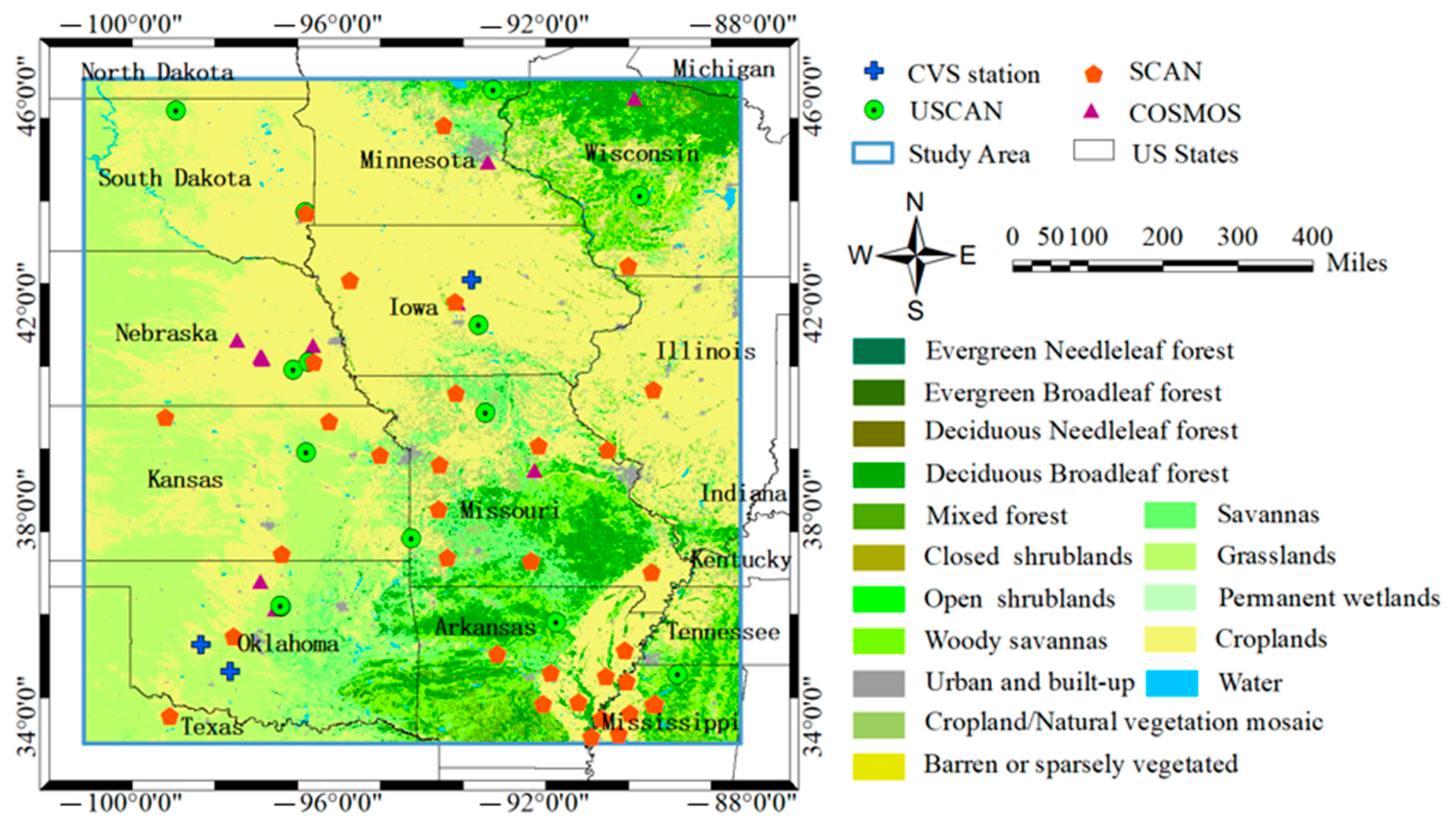
Figure 1 presents the spatial distribution of the in-situ SM observation stations and the study area. It is located in the central United States. The landform of the study area is characterized by a broad expanse of flat land. It has semi-arid continental climate. The dominant land covers include prairie, steppe, and grassland.
The SM observations at sparse networks were obtained from the International Soil Moisture Network (ISMN, https://ismn.geo.tuwien.ac.at/en/). The SM at CVS were obtained from SMAP/In Situ Core Validation Site Land Surface Parameters Match-Up Data, Version 1 [36]. SCAN and USCRN networks provide SM at various depths of measurements. The SM observations at the depth of 0.05m were retained for analysis in order to match the measurement depth of remotely sensed SM by SMAP [37]. The in-situ SM observations are hourly data recorded in Coordinated Universal Time (UTC) time. In order to match the remotely sensed SM, the in-situ SM observations within the local solar time range from 5:00 a.m. to 7:00 a.m. were averaged to match the SMAP SM at 6:00 a.m.
4. Results
In this section, various downscaled SM data with different downscaling factors were compared with original SM, with in-situ SM at CVS, and with in-situ SM at sparse stations. Therefore, the following results are three-fold.
4.1. Evaluation with Original SM
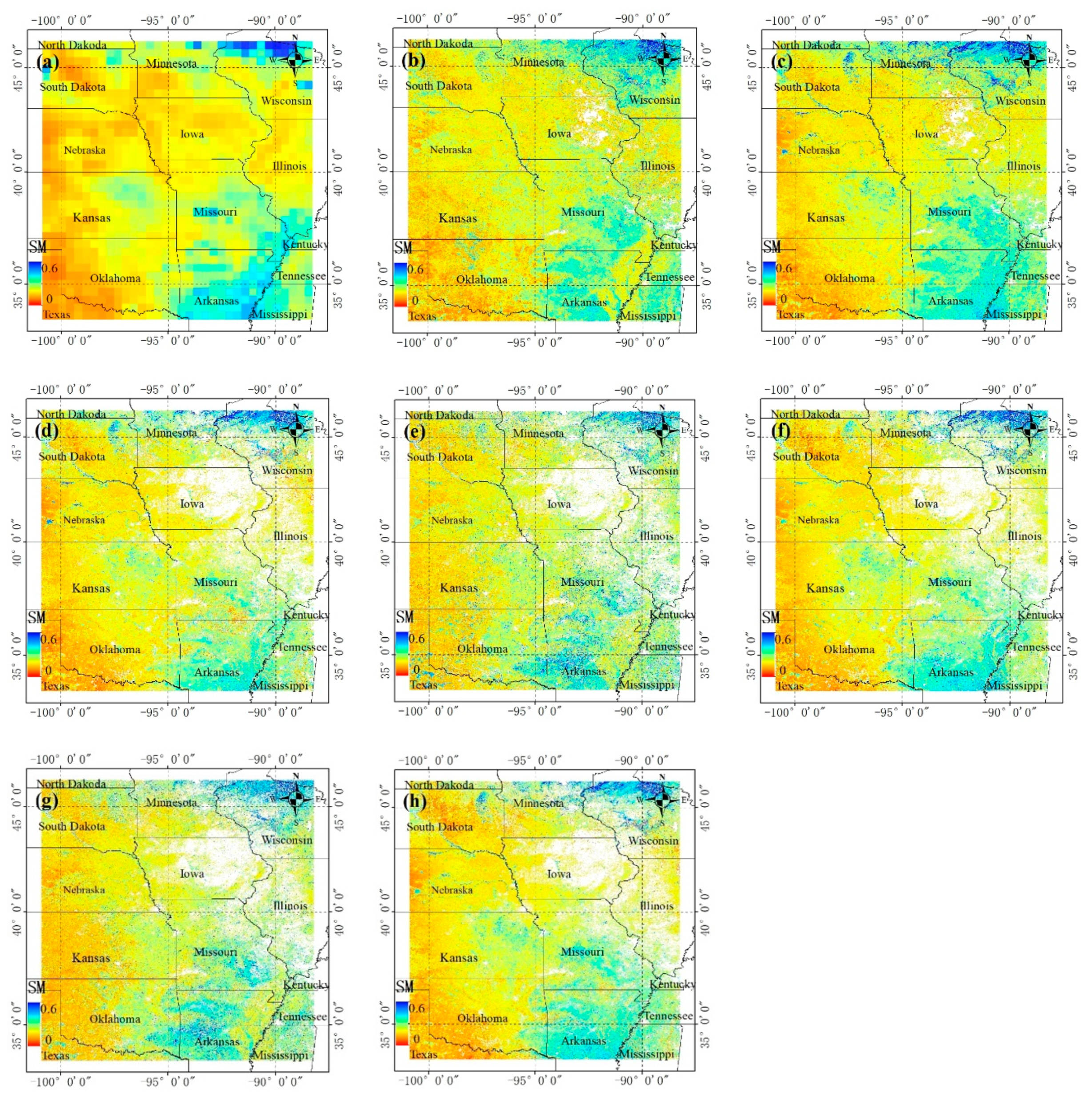
Figure 2 illustrates the spatial distribution of original SM (Figure 2a) and various downscaled SM where (b)~(h) represent the results from Test1 to Test7, taking the data of 27 July 2016 as an example. In the study area, the west area is relatively dry while the northeast and southeast areas are relatively wet, as identified by the original SM. This spatial pattern is retained during the downscaling process, although a difference exists among various downscaled SM data. In order to evaluate the spatial difference between original and downscaled SM quantitatively, we aggregated the downscaled SM into the same spatial resolution as the original SM. Subsequently, the difference between the aggregated SM and original SM was investigated.
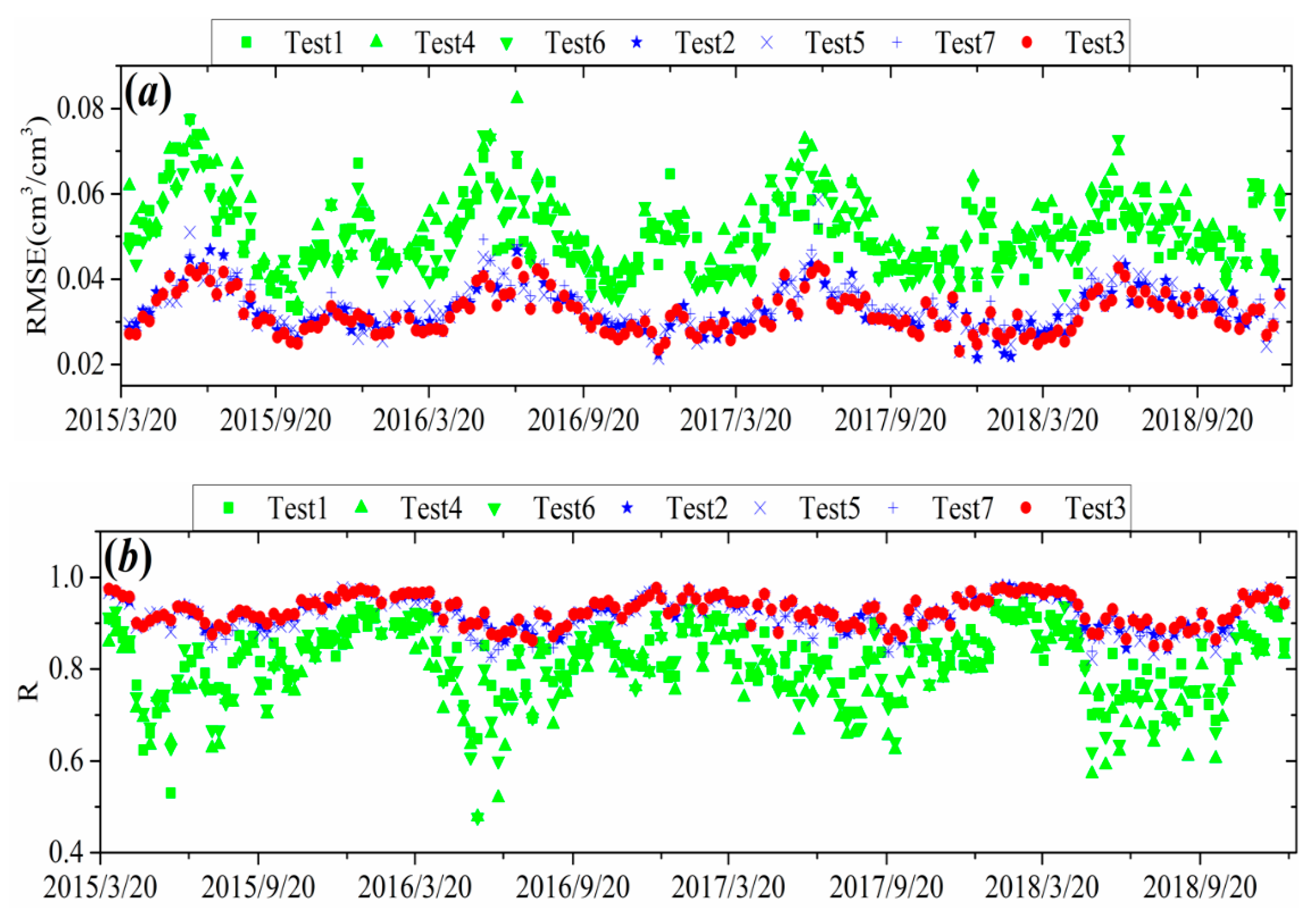
Figure 3 presents the statistics of the difference between original SM and aggregated SM during the whole study period from 2015 to 2018. The indicators RMSE and R were utilized. The greater R and smaller RMSE indicate better performance of the downscaled SM as compared with the original SM. Therefore, we can arrange the various downscaled SM according to the mean of numerous RMSE and R over the whole study period. For RMSE, Test3(0.032) < Test2(0.033) = Test5(0.033) < Test7(0.034) < Test6(0.050) = Test1(0.050) < Test4(0.053). For R, Test3(0.927) > Test2(0.926) > Test5(0.919) > Test7(0.918) > Test1(0.821) > Test6(0.811) > Test4(0.786). The results indicate that Test3 has the best performance, which integrates all of the downscaling factors. Test2, Test5, and Test7 belong to the second tier, which all integrate the geographical indicators. The remaining Test1, Test4, and Test6 are in the third tier, where the geographical indicators are not taken into account. Within the third tier, Test1 and Test6 present very similar performance with the same RMSE and close R. We can also find this phenomenon within the second tier, showing that Test2 and Test5 or Test7 have very similar performance. It should be noted that the only difference between Test1 and Test6 is the difference between LST and LEE. From this mass conservation analysis, we found that adding geographical factors could improve the performance of downscaling SM significantly. We also found that LST and LEE are comparative as downscaling factors. Certainly, more comparisons are required especially the comparison against in-situ SM.
4.2. Evaluation with In Situ SM at CVS
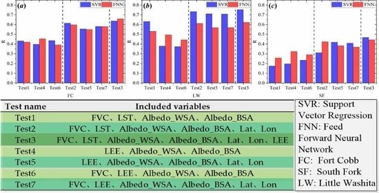
Table 3 shows the comparison of downscaled SM against in-situ SM at three CVS stations: Little Washita (LW), Fort Cobb (FC), and South Fork (SF). RMSE, ubRMSE, and R were used as quantitative indicators. From the indicator of R, we found Test3 got the greatest value at the three CVS stations as compared with the other experiments. The R at FC for Test3 is the highest with 0.637. Test2, Test5, and Test7 are still in the second tier. Again, Test1, Test4, and Test6 are retained in the third tier. Specifically, the R at FC for Test2, Test5, and Test7 are all greater than 0.5. Correspondingly, the R for Test1, Test4, and Test6 are around 0.4. This phenomenon can also be found from the indicators of RMSE and ubRMSE for the stations of FC and SF. There is a little disturbance for station of LW where the first tier (Test3) and the second tier (Test2, Test5, and Test7) are so close that sometimes Test2 is better than Test3. Such disturbance does not change the hierarchical relationship among these experiments. Moreover, the experiments within each hierarchy possess comparative performances, which means that LEE is comparative to LST as downscaling factors. For example, the R values at FC are 0.432 for Test1 and 0.435 for Test6. That values at SF are 0.174 for Test1, 0.197 for Test4, and 0.234 for Test6. We also note that the R value of Test1 is greater than that of Test4 and Test6 at LW, which means that LST is better than LEE at some time.
4.3. Evaluation with In Situ SM at Sparse Stations
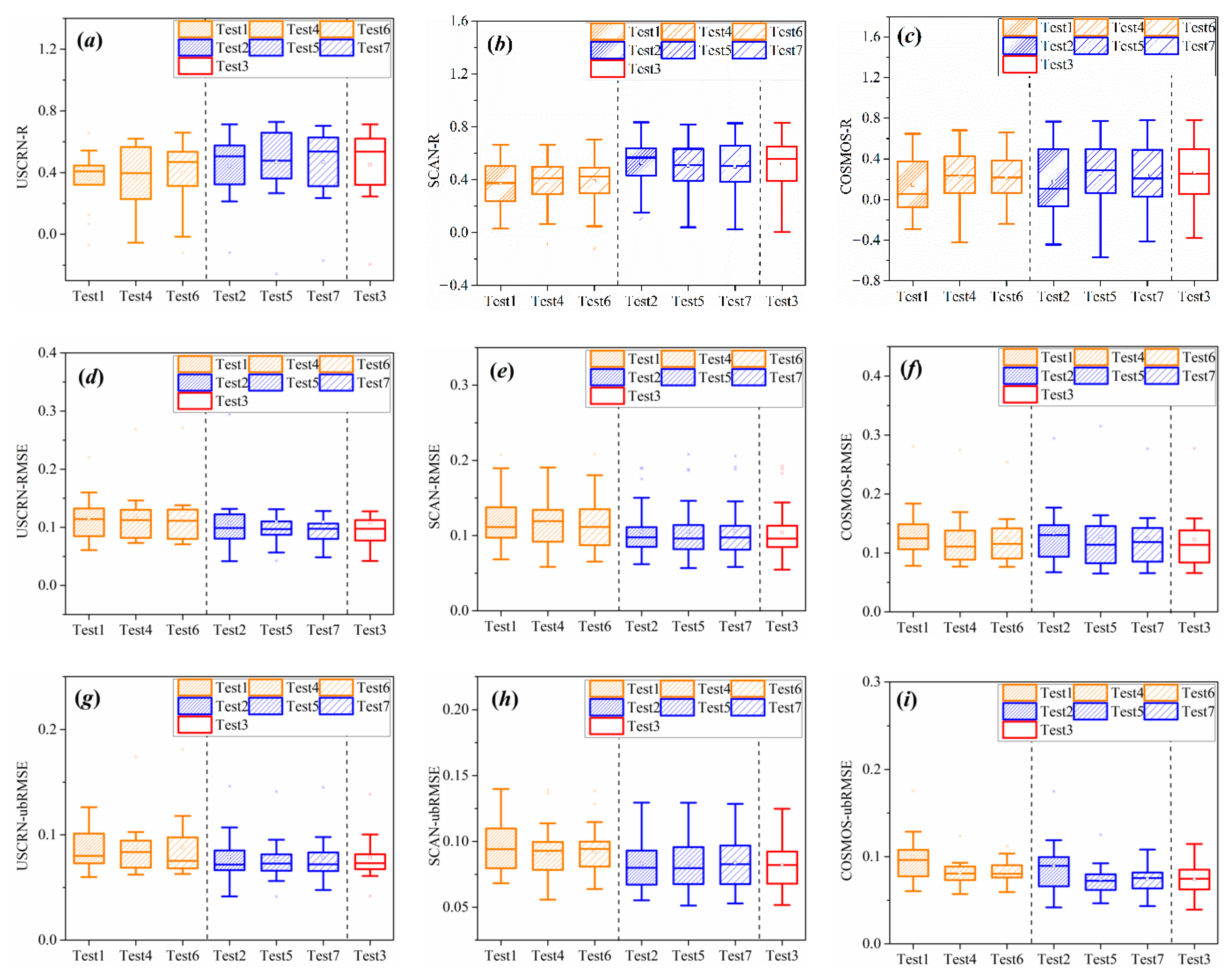
Figure 4 employed box plots to present the comparisons of various downscaled SM with in-situ SM at sparse networks. The above-mentioned hierarchical relationship still exists in the comparisons against these in-situ SM at sparse stations. Taking the results at SCAN for example, we could clearly distinguish the third tier (Test1, Test4, and Test6) from the other experiments. However, the hierarchical relationship is marked at the sparse networks of USCRN and SCAN better than that at the sparse network of COSMOS. This may be because COSMOS probes measure SM at the depths of decimeters [38]. In contrast, the SM observations of SCAN and USCRN at the depth of 0.05 m were employed in this study and this depth has well consistency with the depth of SMAP SM.
In order to show the comparisons more specifically, we present the comparisons at the station of ARM_1 in COSMOS, the station of GoodwinGreekTimber in SCAN, and the station of Stillwater-5-WNW in USCRN. The specific results are listed in Table 4. According to the R indicator in Table 4, Test3 got the highest value for COSMOS station (0.745), SCAN station (0.831), and USCRN station (0.713). As belonging to the second tier, Test2, Test5, and Test7 are greater than 0.6 for COSMOS. Moreover, they are also in the second tier for SCAN and USCRN. The Test1, Test4, and Test6 are in the third tier since their R values are less than 0.6 for COSMOS. They also got a third position for SCAN and USCRN. Again, LEE and LST are comparative as downscaling factors. Sometimes LEE is better and sometimes LST is better.
In summary, we evaluated the downscaling factors through comparing the downscaled SM with original SM and the in-situ SM at CVS and sparse networks. The comparison results indicated a hierarchical relationship among the experiments. The Test3, which integrated the traditional FVC and LST, the LEE, and the geographical factors, has the best performance. The Test2, Test5, and Test7 which all integrated the geographical factors are in the second tier. The Test1, Test4, and Test6 which did not integrate the geographical factors are in the third tier. Moreover, the experiments within each hierarchy possess comparative performances. The results demonstrate that geographical factors can improve the downscaling performance significantly and LEE can be taken as an alternative of LST for downscaling microwave SM.
5. Discussion
The above-mentioned results were obtained with the Z-score normalization method and SVR machine-learning method. Does the other normalization method and machine-learning method can overthrow the study conclusions? With this question, we made the following analysis. Firstly, we compared the Z-score normalization with a hyperbolic-tangent normalization. Secondly, we compared the results with the SVR method and that with the FNN method. The evaluation results are listed as follows.
5.1. Effects of Different Normalization Methods
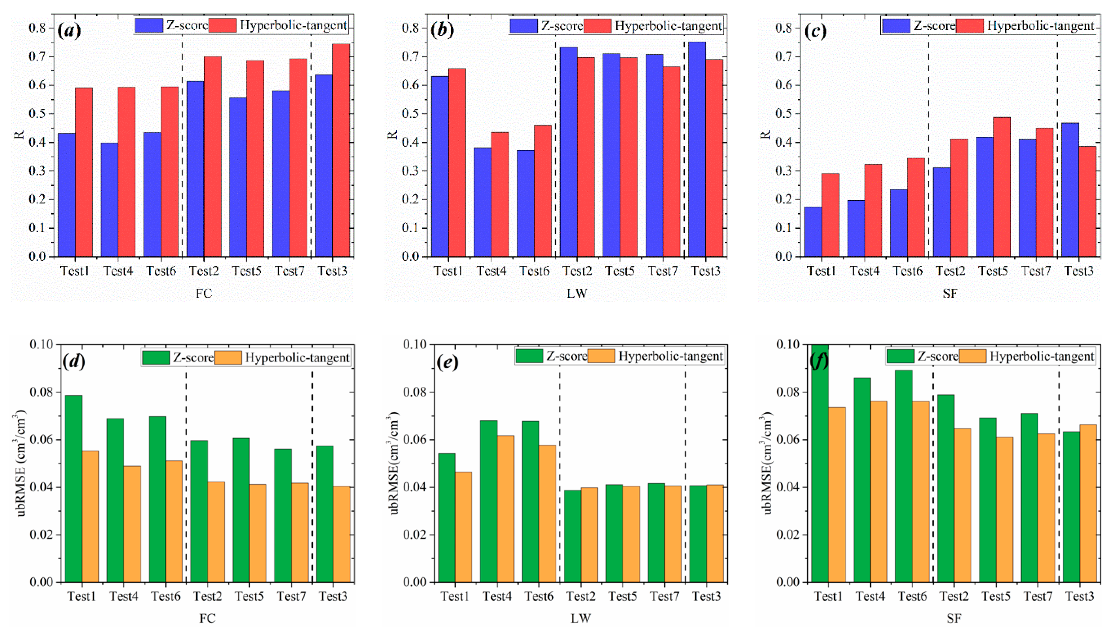
Figure 5 illustrates the comparison between Z-score normalization and hyperbolic-tangent normalization at the three CVS stations FC, LW, and SF. R and ubRMSE are utilized as evaluation indicators. The hierarchy relationship was divided by an ancillary dotted line in this figure. Firstly, the hierarchical relationship among the experiments was maintained when we used whether Z-score normalization or hyperbolic-tangent normalization. Secondly, the experiments within each hierarchy possess comparative performances indicated by both the Z-score normalization and the hyperbolic-tangent normalization. However, we found that the experiment with hyperbolic-tangent normalization showed better performances than that with Z-score normalization in most cases. Consequently, it is recognized that our conclusion does not change no matter Z-score or hyperbolic-tangent normalization was used.
5.2. Effects of Different Machine-Learning Methods
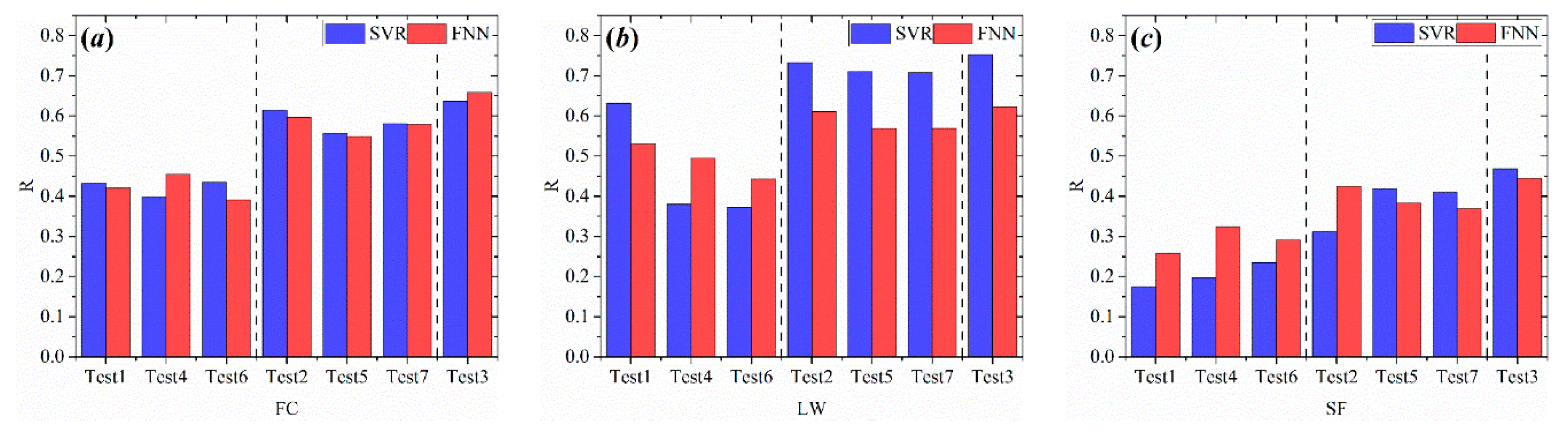
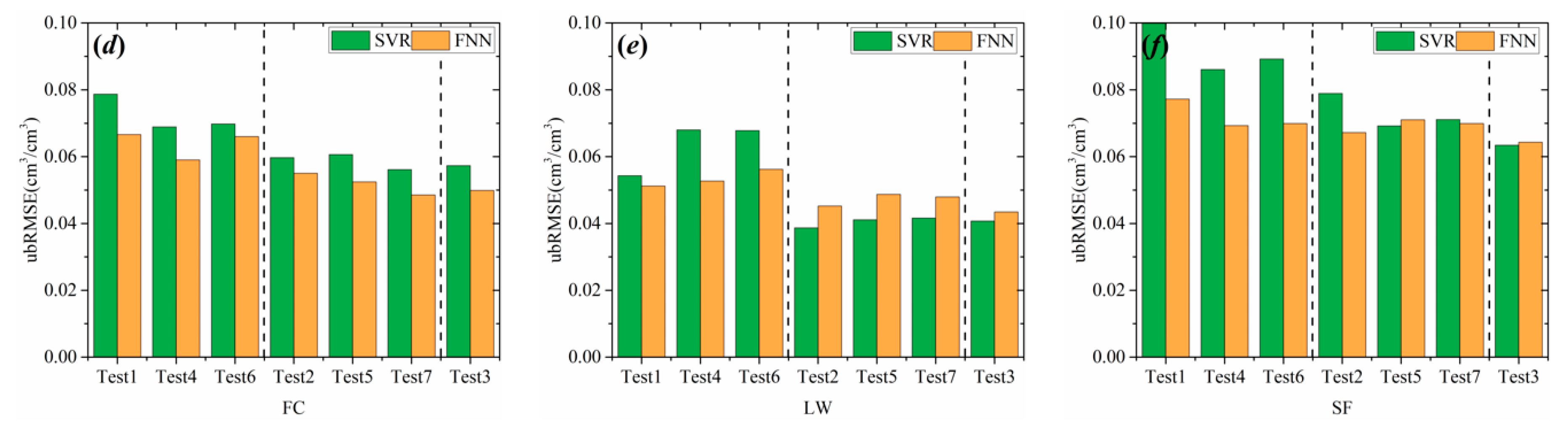
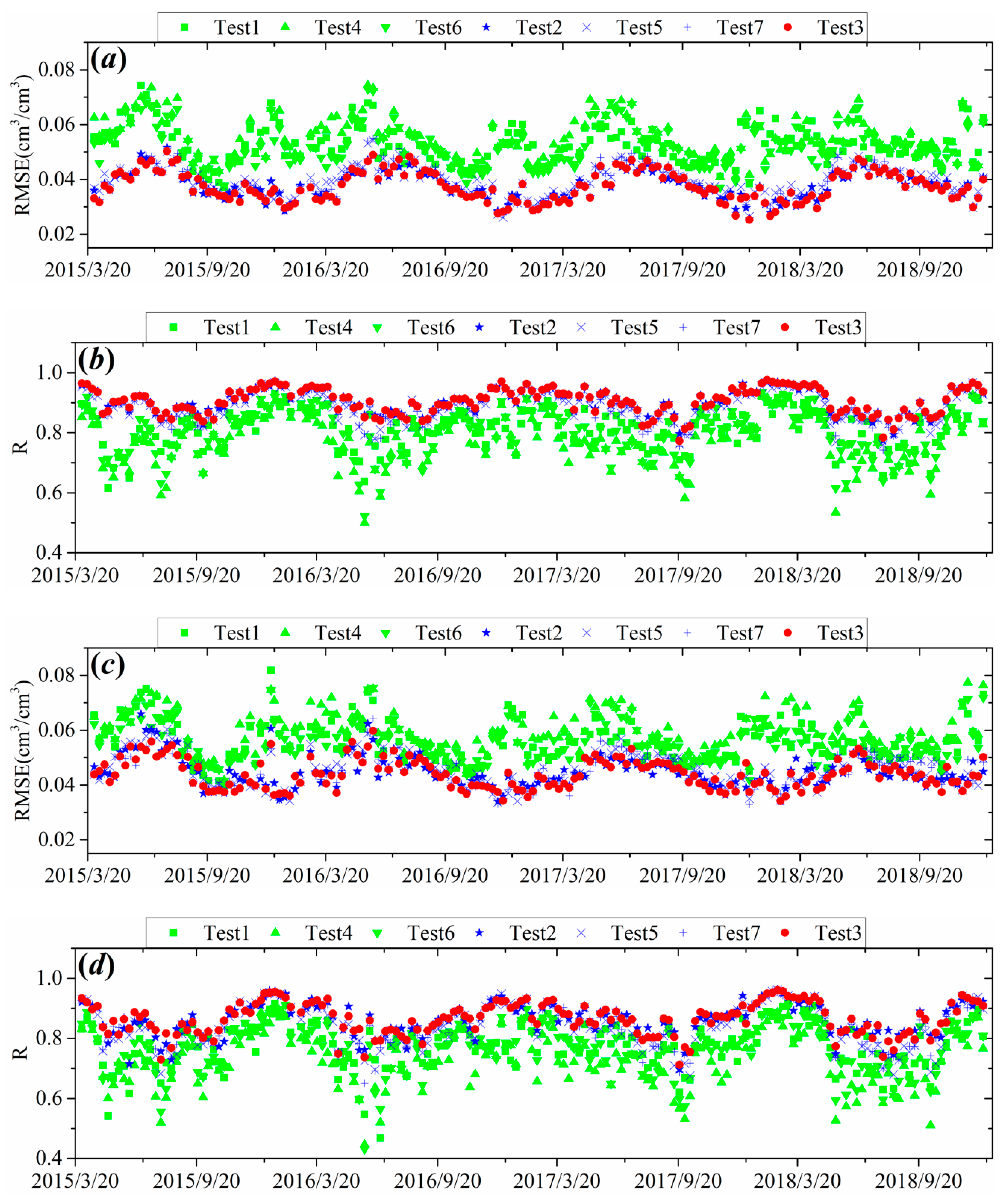
Figure 6 illustrates the comparison between SVR and FNN methods at the CVS stations of FC, LW, and SF. The normalization method used in Figure 6 was consolidated to Z-score. We also use R and ubRMSE as evaluation indicators. Moreover, we compared original SM with aggregated SM for different machine-learning methods and normalization methods. Results are illustrated in Figure 7 where (a) and (b) are RMSE and R values for SVR with hyperbolic-tangent normalization; (c) and (d) are RMSE and R values for FNN with Z-score normalization, respectively. Once again, the comparisons demonstrate that (1) the hierarchical relationship among the experiments was maintained for whether SVR method or FNN method and either for Z-score and hyperbolic-tangent normalization; (2) the experiments within each hierarchy possess comparative performances.
5.3. Implications of the Results
In the era of big data, integrating the plentiful data of optical/thermal remote sensing with microwave remote sensing has a wide range of application to obtain high-resolution SM data (better than 1 km). The downscaling factors are very significant within the downscaling process since they determine the spatial variations within a coarse-resolution SM pixel. LST was indispensable in most downscaling algorithms since LST is as an effective indicator of SM variation. However, LST often cannot be obtained from thermal remote sensing because the influence of the weather conditions. Sun, Cai, Liu, and Yang [12] provided a solution to this problem by introducing gridded meteorological data based on the complementary relationship hypothesis. Although the solution was demonstrated valid for downscaling SMAP SM of 36 km into 4 km, the spatial resolution of gridded meteorological data is still too coarse as compared with LST of 1 km in MODIS products. The main contribution of this study is demonstrating the possibility of using LEE from MODIS-MOD16 dataset as an alternative when there is no available LST data for downscaling. The LEE from MODIS-MOD16 has the highest spatial resolution of 500 m which can be compared with the LST of 1 km. This contribution is particularly useful with the releasing of gap-filled MOD16 data, i.e., the MOD16A3GF, which implies that it can be used for all-weather SM downscaling.
However, it should be noted that LST is a very valuable piece of information. In this study, we found that integrating LST and LEE can get better performance than utilizing one of them independently. Consequently, this study does not mean that LEE can be used to replace LST for SM downscaling. In contrast, we encourage to integrate LEE and LST to obtain spatial continuous downscaling factors in order to match the spatial continuous microwave data.
In addition, this study demonstrates that it is valid and necessary to add geographical factors within the downscaling process. Currently, geographical factors have been employed in statistical regression downscaling method. However, they are rarely used in physical model or parameterized model of downscaling microwave SM. The future physical model, parameterized model, or their combinations with ML methods should incorporate the geographical factors.
Moreover, there are some studies attempting to fill the gap of LST due to cloud contamination through using spatiotemporal neighbor LST information [39] or other supplementary factors [40]. Therefore, in the future, integrating spatial-continuous LST, LEE, and geographical factors would greatly promote the performance of downscaling microwave satellite SM.
6. Conclusions
This study evaluated several typical downscaling factors of microwave satellite SM. Seven groups of experiments with different combinations of downscaling factors were constructed and evaluated based on a machine learning method SVR and Z-score normalization method. Original SM from SMAP satellite and in situ SM at sparse networks and CVS stations were used as reference. Results indicated that there exist hierarchy relationships among the seven experimental groups. The group that integrated LST, LEE, and the geographical factors has the best performance. The groups that integrated geographical factors is better than that without geographical factors. In addition, LEE presents comparative performance to LST as downscaling factors. The above results do not change when another machine learning method FNN or hyperbolic-tangent normalization method was utilized. This study contributes experimental evidences to that LEE can be taken as an alternative of LST for downscaling microwave SM and geographical factors can improve the downscaling performance significantly. The future work is expected to integrate the LEE, LST, and geographical factors for obtaining high-resolution SM from the fusion of SMAP and MODIS.
Author Contributions
Conceptualization, H.S.; methodology, H.S.; formal analysis, Y.C.; writing—original draft preparation, H.S. and Y.C.; resources, Y.C.; writing—review and editing, H.S. and Y.C. All authors have read and agreed to the published version of the manuscript.
Funding
This research was funded by National Natural Science Foundation of China, grant number 41871338 and 41771448; Ningxia Key Research and Development Program, grant number 2018BEG03069; Yue Qi Young Scholar Project, CUMTB2018; and Fundamental Research Funds for the Central Universities, grant number 2020YJSDC08.
Data Availability Statement
All data presented in this study are available in a publicly accessible repository. Specifically, the SMAP products presented in this study are openly available in NASA Earthdata Search at https://0-doi-org.brum.beds.ac.uk/10.5067/EVYDQ32FNWTH. The MODIS products presented in this study are openly available in NASA Earthdata Search at https://0-doi-org.brum.beds.ac.uk/10.5067/MODIS/MCD15A2H.006, https://0-doi-org.brum.beds.ac.uk/10.5067/MODIS/MCD43A3.006, https://0-doi-org.brum.beds.ac.uk/10.5067/MODIS/MOD11A1.006, https://0-doi-org.brum.beds.ac.uk/10.5067/MODIS/MOD16A2.006, and https://0-doi-org.brum.beds.ac.uk/10.5067/MODIS/MOD09A1.006.
Acknowledgments
The authors would like to thank NASA Distributed Active Archive Center at NSIDC and NASA Land Processes Distributed Active Archive Center for providing the SMAP and MODIS data.
Conflicts of Interest
The authors declare no conflict of interest.
References
- Dobriyal, P.; Qureshi, A.; Badola, R.; Hussain, S.A. A review of the methods available for estimating soil moisture and its implications for water resource management. J. Hydrol. 2012, 458, 110–117. [Google Scholar] [CrossRef]
- AghaKouchak, A.; Farahmand, A.M.; Melton, F.S.; Teixeira, J.P.; Anderson, M.C.; Wardlow, B.D.; Hain, C.R. Remote sensing of drought: Progress, challenges and opportunities. Rev. Geophys. 2015, 53, 452–480. [Google Scholar] [CrossRef] [Green Version]
- Sun, H.; Zhao, X.; Chen, Y.; Gong, A.; Yang, J. A new agricultural drought monitoring index combining MODIS NDWI and day–night land surface temperatures: A case study in China. Int. J. Remote Sens. 2013, 34, 8986–9001. [Google Scholar] [CrossRef]
- Pablos, M.; Martínez-Fernández, J.; Sanchez, N.; González-Zamora, Á. Temporal and spatial comparison of agricultural drought indices from moderate resolution satellite soil moisture data over northwest Spain. Remote Sens. 2017, 9, 1168. [Google Scholar] [CrossRef] [Green Version]
- Robinson, D.A.; Campbell, C.S.; Hopmans, J.W.; Hornbuckle, B.K.; Jones, S.B.; Knight, R.; Ogden, F.; Selker, J.; Wendroth, O. Soil moisture measurement for ecological and hydrological watershed-scale observatories: A review. Vadose Zone J. 2008, 7, 358–389. [Google Scholar] [CrossRef] [Green Version]
- Anderson, M.; Norman, J.M.; Mecikalski, J.R.; Otkin, J.A.; Kustas, W.P. A climatological study of evapotranspiration and moisture stress across the continental United States based on thermal remote sensing: 2. Surface moisture climatology. J. Geophys. Res. Atmos. 2007, 112, D11112. [Google Scholar] [CrossRef]
- Dorigo, W.; Wagner, W.; Hohensinn, R.; Hahn, S.; Paulik, C.; Xaver, A.; Gruber, A.; Drusch, M.; Mecklenburg, S.; van Oevelen, P.; et al. The International Soil Moisture Network: A data hosting facility for global in situ soil moisture measurements. Hydrol. Earth Syst. Sci. 2011, 15, 1675–1698. [Google Scholar] [CrossRef] [Green Version]
- Gruber, A.; Dorigo, W.; Zwieback, S.; Xaver, A.; Wagner, W. Characterizing coarse-scale representativeness of in situ soil moisture measurements from the international soil moisture network. Vadose Zone J. 2013, 12, 1–16. [Google Scholar] [CrossRef] [Green Version]
- Ochsner, T.E.; Cosh, M.H.; Cuenca, R.H.; Dorigo, W.A.; Draper, C.S.; Hagimoto, Y.; Kerr, Y.H.; Larson, K.M.; Njoku, E.G.; Small, E.E.; et al. State of the art in large-scale soil moisture monitoring. Soil Sci. Soc. Am. J. 2013, 77, 1888–1919. [Google Scholar] [CrossRef] [Green Version]
- Babaeian, E.; Sadeghi, M.; Jones, S.B.; Montzka, C.; Vereecken, H.; Tuller, M. Ground, proximal, and satellite remote sensing of soil moisture. Rev. Geophys. 2019, 57, 530–616. [Google Scholar] [CrossRef] [Green Version]
- Das, N.N.; Entekhabi, D.; Njoku, E.G. An algorithm for merging SMAP radiometer and radar data for high-resolution soil-moisture retrieval. IEEE Trans. Geosci. Remote Sens. 2011, 49, 1504–1512. [Google Scholar] [CrossRef]
- Sun, H.; Cai, C.; Liu, H.; Yang, B. Microwave and meteorological fusion: A method of spatial downscaling of remotely sensed soil moisture. IEEE J. Sel. Top. Appl. Earth Obs. Remote Sens. 2019, 12, 1107–1119. [Google Scholar] [CrossRef]
- Sun, H.; Zhou, B.; Liu, H. Spatial evaluation of soil moisture (SM), land surface temperature (LST), and LST-derived SM indexes dynamics during SMAPVEX12. Sensors 2019, 19, 1247. [Google Scholar] [CrossRef] [PubMed] [Green Version]
- Peng, J.; Loew, A.; Merlin, O.; Verhoest, N.E.C. A review of spatial downscaling of satellite remotely sensed soil moisture. Rev. Geophys. 2017, 55, 341–366. [Google Scholar] [CrossRef]
- Chauhan, N.S.; Miller, S.; Ardanuy, P. Spaceborne soil moisture estimation at high resolution: A microwave-optical/IR synergistic approach. Int. J. Remote Sens. 2003, 24, 4599–4622. [Google Scholar] [CrossRef]
- Merlin, O.; Walker, J.; Chehbouni, A.; Kerr, Y. Towards deterministic downscaling of SMOS soil moisture using MODIS derived soil evaporative efficiency. Remote Sens. Environ. 2008, 112, 3935–3946. [Google Scholar] [CrossRef] [Green Version]
- Merlin, O.; Rudiger, C.; Al Bitar, A.; Richaume, P.; Walker, J.P.; Kerr, Y.H. Disaggregation of SMOS soil moisture in Southeastern Australia. IEEE Trans. Geosci. Remote Sens. 2012, 50, 1556–1571. [Google Scholar] [CrossRef] [Green Version]
- Merlin, O.; Al Bitar, A.; Walker, J.P.; Kerr, Y. An improved algorithm for disaggregating microwave-derived soil moisture based on red, near-infrared and thermal-infrared data. Remote Sens. Environ. 2010, 114, 2305–2316. [Google Scholar] [CrossRef] [Green Version]
- Merlin, O.; Olivera-Guerra, L.; Hssaine, B.A.; Amazirh, A.; Rafi, Z.; Ezzahar, J.; Gentine, P.; Khabba, S.; Gascoin, S.; Er-Raki, S. A phenomenological model of soil evaporative efficiency using surface soil moisture and temperature data. Agric. For. Meteorol. 2018, 501–515. [Google Scholar] [CrossRef] [Green Version]
- Kim, J.; Hogue, T.S. Improving spatial soil moisture representation through integration of AMSR-E and MODIS products. IEEE Trans. Geosci. Remote Sens. 2012, 50, 446–460. [Google Scholar] [CrossRef]
- Njoku, E.; Wilson, W.; Yueh, S.; Dinardo, S.; Li, F.; Jackson, T.; Lakshmi, V.; Bolten, J. Observations of soil moisture using a passive and active low-frequency microwave airborne sensor during SGP99. IEEE Trans. Geosci. Remote Sens. 2002, 40, 2659–2673. [Google Scholar] [CrossRef]
- Sun, H.; Zhou, B.; Zhang, C.; Liu, H.; Yang, B. DSCALE_mod16: A model for disaggregating microwave satellite soil moisture with land surface evapotranspiration products and gridded meteorological data. Remote Sens. 2020, 12, 980. [Google Scholar] [CrossRef] [Green Version]
- Wagner, W.; Blöschl, G.; Pampaloni, P.; Calvet, J.-C.; Bizzarri, B.; Wigneron, J.-P.; Kerr, Y. Operational readiness of microwave remote sensing of soil moisture for hydrologic applications. Hydrol. Res. 2007, 38, 1–20. [Google Scholar] [CrossRef]
- Yuan, Q.; Shen, H.; Li, T.; Li, Z.; Li, S.; Jiang, Y.; Xu, H.; Tan, W.; Yang, Q.; Wang, J.; et al. Deep learning in environmental remote sensing: Achievements and challenges. Remote Sens. Environ. 2020, 241, 111716. [Google Scholar] [CrossRef]
- Zhan, X.; Miller, S.; Chauhan, N.; Di, L.; Ardanuy, P. Soil Moisture Visible/Infrared Radiometer Suite Algorithm Theoretical Basis Document; Raytheon Syst. Company: Lanham, MD, USA, 2002. [Google Scholar]
- Srivastava, P.K.; Han, D.; Ramirez, M.A.R.; Islam, T. Machine learning techniques for downscaling SMOS satellite soil moisture using MODIS land surface temperature for hydrological application. Water Resour. Manag. 2013, 27, 3127–3144. [Google Scholar] [CrossRef]
- Cui, Y.; Chen, X.; Xiong, W.; He, L.; Lv, F.; Fan, W.; Luo, Z.; Hong, Y. A soil moisture spatial and temporal resolution improving algorithm based on multi-source remote sensing data and GRNN model. Remote Sens. 2020, 12, 455. [Google Scholar] [CrossRef] [Green Version]
- Remesan, R.; Shamim, M.A.; Han, D.; Mathew, J. Runoff prediction using an integrated hybrid modelling scheme. J. Hydrol. 2009, 372, 48–60. [Google Scholar] [CrossRef]
- Liu, Y.; Jing, W.; Wang, Q.; Xia, X. Generating high-resolution daily soil moisture by using spatial downscaling techniques: A comparison of six machine learning algorithms. Adv. Water Resour. 2020, 141, 103601. [Google Scholar] [CrossRef]
- Peng, J.; Loew, A.; Zhang, S.; Wang, J.; Niesel, J. Spatial downscaling of satellite soil moisture data using a vegetation temperature condition index. IEEE Trans. Geosci. Remote Sens. 2016, 54, 558–566. [Google Scholar] [CrossRef]
- Peng, J.; Niesel, J.; Loew, A. Evaluation of soil moisture downscaling using a simple thermal-based proxythe—The REMEDHUS network (Spain) example. Hydrol. Earth Syst. Sci. 2015, 19, 4765–4782. [Google Scholar] [CrossRef] [Green Version]
- Chen, Q.; Miao, F.; Wang, H.; Xu, Z.; Tang, Z.; Yang, L.; Qi, S. Downscaling of satellite remote sensing soil moisture products over the Tibetan Plateau based on the random forest algorithm: Preliminary results. Earth Space Sci. 2020, 7, e2020EA001265. [Google Scholar] [CrossRef]
- Zappa, L.; Forkel, M.; Xaver, A.; Dorigo, W. Deriving field scale soil moisture from satellite observations and ground measurements in a hilly agricultural region. Remote Sens. 2019, 11, 2596. [Google Scholar] [CrossRef] [Green Version]
- Roujean, J.-L.; Leroy, M.; Deschamps, P.-Y. A bidirectional reflectance model of the Earth’s surface for the correction of remote sensing data. J. Geophys. Res. 1992, 97, 20455–20468. [Google Scholar] [CrossRef]
- Mu, Q.; Zhao, M.; Running, S.W. Improvements to a MODIS global terrestrial evapotranspiration algorithm. Remote Sens. Environ. 2011, 115, 1781–1800. [Google Scholar] [CrossRef]
- SMAP/In Situ Core Validation Site Land Surface Parameters Match-Up Data, Version 1; NASA National Snow and Ice Data Center Distributed Active Archive Center: Boulder, CO, USA, 2017. Available online: https://nsidc.org/data/NSIDC-0712/versions/1 (accessed on 1 January 2021).
- Entekhabi, D.; Yueh, S.; O’Neill, P.E.; Kellogg, K.H.; Allen, A.; Bindlish, R.; Brown, M.; Chan, S.; Colliander, A.; Crow, W.T.; et al. SMAP Handbook-Soil Moisture Active Passive: Mapping Soil Moisture and Freeze/Thaw from Space; JPL Publication: Pasadena, CA, USA, 2014.
- Montzka, C.; Bogena, H.; Zreda, M.; Monerris, A.; Morrison, R.; Muddu, S.; Vereecken, H. Validation of spaceborne and modelled surface soil moisture products with cosmic-ray neutron probes. Remote Sens. 2017, 9, 103. [Google Scholar] [CrossRef] [Green Version]
- Li, X.; Zhou, Y.; Asrar, G.R.; Zhu, Z. Creating a seamless 1 km resolution daily land surface temperature dataset for urban and surrounding areas in the conterminous United States. Remote Sens. Environ. 2018, 206, 84–97. [Google Scholar] [CrossRef]
- Shwetha, H.R.; Kumar, D.N. Prediction of high spatio-temporal resolution land surface temperature under cloudy conditions using microwave vegetation index and ANN. ISPRS J. Photogramm. Remote Sens. 2016, 117, 40–55. [Google Scholar] [CrossRef]
Figure 1.
Spatial distribution of the in-situ soil moisture (SM) observation stations and the study area.
Figure 1.
Spatial distribution of the in-situ soil moisture (SM) observation stations and the study area.

Figure 2.
Original and downscaled SM (cm3/cm3) on July 27, 2016, where (a) is original 36 km SM; (b–h) are the downscaled results with Test1 to Test7, respectively.
Figure 2.
Original and downscaled SM (cm3/cm3) on July 27, 2016, where (a) is original 36 km SM; (b–h) are the downscaled results with Test1 to Test7, respectively.

Figure 3.
Statistics of the difference between original SM and aggregated SM for Support Vector Regression (SVR) with Z-score normalization during the whole study period from 2015 to 2018. (a,b) are the indicators of RMSE and R, respectively.
Figure 3.
Statistics of the difference between original SM and aggregated SM for Support Vector Regression (SVR) with Z-score normalization during the whole study period from 2015 to 2018. (a,b) are the indicators of RMSE and R, respectively.

Figure 4.
Box plots of the comparisons between various downscaled SM data and in-situ SM at sparse networks. (a–c) are R values for the three sparse networks USCRN, SCAN, and COSMOS, respectively. (d–f) are RMSE (cm3/cm3) for the three sparse networks. (g–i) are ubRMSE (cm3/cm3) for the three sparse networks.

Figure 5.
Comparison of Z-score normalization against hyperbolic-tangent normalization at three CVS stations where (a–c) are R values and (d–f) are ubRMSE values at FC, LW, and SF, respectively.
Figure 5.
Comparison of Z-score normalization against hyperbolic-tangent normalization at three CVS stations where (a–c) are R values and (d–f) are ubRMSE values at FC, LW, and SF, respectively.

Figure 6.
Comparison of SVR method against FNN method at three CVS stations where (a–c) are R values and (d–f) are ubRMSE values at FC, LW, and SF, respectively.
Figure 6.
Comparison of SVR method against FNN method at three CVS stations where (a–c) are R values and (d–f) are ubRMSE values at FC, LW, and SF, respectively.


Figure 7.
Comparison between original SM and aggregated SM for different machine-learning and normalization methods. (a,b) are RMSE and R values for SVR with hyperbolic-tangent normalization; (c,d) are RMSE and R values for FNN with Z-score normalization, respectively.
Figure 7.
Comparison between original SM and aggregated SM for different machine-learning and normalization methods. (a,b) are RMSE and R values for SVR with hyperbolic-tangent normalization; (c,d) are RMSE and R values for FNN with Z-score normalization, respectively.


Table 1.
Seven groups of experiment conducted in this study where Albedo_WSA and Albedo_BSA are white and black sky albedo, respectively. Lat and Lon are abbreviations of latitude and longitude.
Table 1.
Seven groups of experiment conducted in this study where Albedo_WSA and Albedo_BSA are white and black sky albedo, respectively. Lat and Lon are abbreviations of latitude and longitude.
| Test Name | Included Variables |
|---|---|
| Test1 | FVC, LST, Albedo_WSA, Albedo_BSA |
| Test2 | FVC, LST, Albedo_WSA, Albedo_BSA, Lat, Lon |
| Test3 | FVC, LST, Albedo_WSA, Albedo_BSA, Lat, Lon, LEE |
| Test4 | LEE, Albedo_WSA, Albedo_BSA |
| Test5 | LEE, Albedo_WSA, Albedo_BSA, Lat, Lon |
| Test6 | FVC, LEE, Albedo_WSA, Albedo_BSA |
| Test7 | FVC, LEE, Albedo_WSA, Albedo_BSA, Lat, Lon |
Table 2.
Moderate Resolution Imaging Spectroradiometer (MODIS)-derived Variables that used in this study.
Table 2.
Moderate Resolution Imaging Spectroradiometer (MODIS)-derived Variables that used in this study.
| Data | MODIS Product | Unit | Temporal Resolution | Spatial Resolution |
|---|---|---|---|---|
| Albedo | MCD43A3 | N/A | daily | 500 m |
| Land Surface Temperature (LST) | MOD11A1 | Kelvin | daily | 1 km |
| LE | MOD16A2 | J/m²/day | 8-day | 500 m |
| PLE | MOD16A2 | J/m²/day | 8-day | 500 m |
| Leaf area index (LAI) | MOD15A2H | m²/m² | 8-day | 500 m |
| ϑ | MOD09A1 | degree | 8-day | 500 m |
Table 3.
Comparison of various downscaled SM data against in-situ SM at Core Validation Sites (CVS) where LW, FC, and SF are Little Washita, Fort Cobb, and South Fork, respectively.
Table 3.
Comparison of various downscaled SM data against in-situ SM at Core Validation Sites (CVS) where LW, FC, and SF are Little Washita, Fort Cobb, and South Fork, respectively.
| RMSE (cm3/cm3) | ubRMSE (cm3/cm3) | R | |||||||
|---|---|---|---|---|---|---|---|---|---|
| FC | LW | SF | FC | LW | SF | FC | LW | SF | |
| Test1 | 0.083 | 0.061 | 0.101 | 0.079 | 0.054 | 0.100 | 0.432 | 0.631 | 0.174 |
| Test4 | 0.073 | 0.079 | 0.086 | 0.069 | 0.068 | 0.086 | 0.397 | 0.379 | 0.197 |
| Test6 | 0.077 | 0.073 | 0.090 | 0.070 | 0.068 | 0.089 | 0.435 | 0.373 | 0.234 |
| Test2 | 0.065 | 0.039 | 0.084 | 0.060 | 0.039 | 0.079 | 0.614 | 0.733 | 0.311 |
| Test5 | 0.068 | 0.042 | 0.070 | 0.061 | 0.041 | 0.069 | 0.556 | 0.710 | 0.418 |
| Test7 | 0.064 | 0.043 | 0.072 | 0.056 | 0.042 | 0.071 | 0.580 | 0.708 | 0.409 |
| Test3 | 0.063 | 0.041 | 0.067 | 0.057 | 0.041 | 0.063 | 0.637 | 0.753 | 0.468 |
Table 4.
Comparison of various downscaled SM data against in-situ SM at the station of ARM_1 in Cosmic-ray Soil Moisture Observing System (COSMOS), the station of GoodwinGreekTimber in U.S. Department of Agriculture Soil Climate Analysis Network (SCAN), and the station of Stillwater-5-WNW in U.S. Climate Reference Network (USCRN).
| RMSE (cm3/cm3) | ubRMSE (cm3/cm3) | R | |||||||
|---|---|---|---|---|---|---|---|---|---|
| COSMOS | SCAN | USCRN | COSMOS | SCAN | USCRN | COSMOS | SCAN | USCRN | |
| Test1 | 0.086 | 0.120 | 0.061 | 0.078 | 0.088 | 0.060 | 0.598 | 0.563 | 0.656 |
| Test4 | 0.082 | 0.120 | 0.073 | 0.075 | 0.086 | 0.068 | 0.490 | 0.629 | 0.457 |
| Test6 | 0.084 | 0.106 | 0.071 | 0.078 | 0.075 | 0.070 | 0.556 | 0.701 | 0.535 |
| Test2 | 0.068 | 0.102 | 0.042 | 0.053 | 0.058 | 0.042 | 0.725 | 0.816 | 0.706 |
| Test5 | 0.073 | 0.114 | 0.042 | 0.059 | 0.068 | 0.040 | 0.672 | 0.774 | 0.728 |
| Test7 | 0.073 | 0.111 | 0.048 | 0.059 | 0.058 | 0.048 | 0.678 | 0.825 | 0.680 |
| Test3 | 0.071 | 0.110 | 0.042 | 0.055 | 0.058 | 0.042 | 0.745 | 0.831 | 0.713 |
Publisher’s Note: MDPI stays neutral with regard to jurisdictional claims in published maps and institutional affiliations. |
© 2021 by the authors. Licensee MDPI, Basel, Switzerland. This article is an open access article distributed under the terms and conditions of the Creative Commons Attribution (CC BY) license (http://creativecommons.org/licenses/by/4.0/).
Share and Cite
MDPI and ACS Style
Sun, H.; Cui, Y. Evaluating Downscaling Factors of Microwave Satellite Soil Moisture Based on Machine Learning Method. Remote Sens. 2021, 13, 133. https://0-doi-org.brum.beds.ac.uk/10.3390/rs13010133
AMA Style
Sun H, Cui Y. Evaluating Downscaling Factors of Microwave Satellite Soil Moisture Based on Machine Learning Method. Remote Sensing. 2021; 13(1):133. https://0-doi-org.brum.beds.ac.uk/10.3390/rs13010133
Chicago/Turabian StyleSun, Hao, and Yajing Cui. 2021. "Evaluating Downscaling Factors of Microwave Satellite Soil Moisture Based on Machine Learning Method" Remote Sensing 13, no. 1: 133. https://0-doi-org.brum.beds.ac.uk/10.3390/rs13010133
Note that from the first issue of 2016, this journal uses article numbers instead of page numbers. See further details here.