RSCNN: A CNN-Based Method to Enhance Low-Light Remote-Sensing Images


1
School of Earth Sciences, Zhejiang University, Hangzhou 310027, China
2
Zhejiang Provincial Key Laboratory of Geographic Information Science, Hangzhou 310028, China
3
Ocean Academy, Zhejiang University, Zhoushan 316021, China
*
Author to whom correspondence should be addressed.
Remote Sens. 2021, 13(1), 62; https://0-doi-org.brum.beds.ac.uk/10.3390/rs13010062
Submission received: 23 November 2020
/
Revised: 16 December 2020
/
Accepted: 22 December 2020
/
Published: 26 December 2020
(This article belongs to the Special Issue Deep Learning in Remote Sensing: Sample Datasets, Algorithms and Applications)
Abstract
:Image enhancement (IE) technology can help enhance the brightness of remote-sensing images to obtain better interpretation and visualization effects. Convolutional neural networks (CNN), such as the Low-light CNN (LLCNN) and Super-resolution CNN (SRCNN), have achieved great success in image enhancement, image super resolution, and other image-processing applications. Therefore, we adopt CNN to propose a new neural network architecture with end-to-end strategy for low-light remote-sensing IE, named remote-sensing CNN (RSCNN). In RSCNN, an upsampling operator is adopted to help learn more multi-scaled features. With respect to the lack of labeled training data in remote-sensing image datasets for IE, we use real natural image patches to train firstly and then perform fine-tuning operations with simulated remote-sensing image pairs. Reasonably designed experiments are carried out, and the results quantitatively show the superiority of RSCNN in terms of structural similarity index (SSIM) and peak signal-to-noise ratio (PSNR) over conventional techniques for low-light remote-sensing IE. Furthermore, the results of our method have obvious qualitative advantages in denoising and maintaining the authenticity of colors and textures.
1. Introduction
Remote-sensing images play a significant role in large-scale spatial analysis and visualization, including climate change detection [1], urban 3D modelling [2], and global surface monitoring [3]. However, due to the effects of remotely sensed devices, undesirable weather conditions, such as haze, blizzards, storms, clouds, etc. [4], have a great negative impact on the visibility and interpretability of remote-sensing images. Low-light images create more difficulties for many practical tasks such as marine disaster monitoring and night monitoring. Therefore, it is a great necessity to enhance the contrast and brightness of low-light images automatically when we want to achieve a high-quality remote-sensing image dataset with large scale and long time series.
The purpose of image enhancement (IE) is to improve the visual interpretation of images and to provide better clues for further processing and analyzing [4,5,6]. Over time, many low-light IE methods have been proposed and achieved great success in image processing and remote-sensing fields. Histogram Equalization (HE) [7] and its variants such as Dynamic Histogram Equalization (DHE) [8], Brightness Protecting Dynamic Histogram Equalization (BPDHE) [9], and Contrast Constrained Adaptive Histogram Equalization (CLAHE) [10] are classic traditional contrast-enhancement methods. The purpose of HE is to increase the contrast of the entire image by expanding the dynamic range of the image. It is a global adjustment process without considering the change in brightness, which is prone to local overexposure, color distortion, and poor denoising. This kind of method can automatically obtain images with stronger contrast and better brightness. However, the details in dark areas are not appropriately enhanced [11] and there may be color distortions [12].
Retinex theory has attracted a lot of attention as a biologically meaningful method to enhance low-light images. The basis of Retinex theory is that the color of any object in images is determined by its ability to reflect long-wave (red), medium-wave (green), and short-wave (blue) rays rather than by the reflected light intensity, which means the object’s color is not affected by light inhomogeneity and is consistent. Therefore, Retinex theory decomposes the image into two parts: reflectance and illumination. Single-scale Retinex (SSR) [13] uses a Gaussian filter to estimate the illumination and then to wipe it off to keep the reflection only. Extending SSR, Multi-scale Retinex (MSR) [14] uses a multi-scale Gaussian filter to achieve simultaneous dynamic range compression, but it fails to produce good color rendition. Considering this, in Multi-scale Retinex with Color Restoration (MSRCR) [15], a color recovery factor was added to adjust the color distortion caused by the enhanced contrast in local areas of the image. Additionally, methods like “Low-light Image Enhancement (LIME)” [16] are also based on Retinex theory, but they only estimate the luminance map. LIME embeds the problem of optimizing lighting into the optimization problem, taking into account the fidelity and structure of the image, customizing an optimized objective function and corresponding constraints, and then adopting the traditional Lagrangian multiplier method to solve this optimization problem. Bio-Inspired Multi-Exposure Fusion (BIMEF) fuses multiple exposure images through the camera response model and then uses the image fusion weight matrix obtained by illuminance estimation technology to fuse the input image to obtain the enhanced result [17]. Those methods can obviously enhance details [16,18]. However, when SSR estimates the illumination of the image, it is assumed that the initial illumination slowly changes, that is, the illumination is smooth. However, this is not the case. At the edge of the region where the brightness varies greatly, the illumination is usually not smooth. Therefore, the enhanced images often suffer from halo-like artifacts in high-contrast regions [19]. Other machine-learning methods such as Discrete Wavelet Transform and Singular Value Decomposition (DWT-SVD) [20,21] are commonly used for low-light IE tasks. It uses wavelet transform to decompose the high-low frequency channels of the original image. Each channel is then processed respectively and fused to obtain the final enhancement result based on an inverse DWT (IDWT) operator. However, they are unable to capture deep and abstract features for image recovery, resulting in some color distortion.
The Deep Learning (DL) method provides a new solution for low-light image IE tasks. There are two common patterns of DL-based low-light enhancement methods: one involves light estimation, and the other is direct end-to-end training.
For the first type, the authors of [22] proposed a CNN-based network for weakly illuminated image enhancement. LightenNet is a four-stage model. It firstly estimates the illumination map using a four-convolutional-layer network; then, the same as in [16], Gamma correction and guided image filter are applied for a refined illumination map. Experiments show that LightenNet achieves a better estimated illumination map than LIME, naturally leading to a better enhancing result with Retinex theory. In [23], inspired by Retinex theory, the authors proposed a CNN-based network, named Retinex-Net. It firstly uses a decomposition module to decompose the input image into reflectance and illumination. Then, in the adjustment module, the reflectance channel is processed by a denoise operation and the illumination channel is brightened up via an encoder-decoder-based multi-scale skip-connection subnetwork. Finally, the reconstruction module is applied to fuse the individually processed channels for enhanced results.
The end-to-end type is more common. Low-light Net (LLNet) [24] innovatively extends the work in [25] and proved that the stacked sparse denoising autoencoder based on the training of synthetic data can enhance and denoise low-light images with noise adaptively. Experiments of LLNet show that, as for an end-to-end DL method, the batch size, patch size, and layer complexity of the model all have effects on the enhanced result. Smaller batch sizes tend to help find the global minima during optimization and generate enhanced image with better sharpness, but it may cause worse denoising. Besides, a proper layer size is required to adequately capture the characteristics of training data while reducing the risk of a vanishing gradient as much as possible. Low-light CNN (LLCNN) [26] firstly introduces CNN convolutional layers into low-light IE and achieves better result in terms of peak signal-to-noise ratio (PSNR) and structural similarity index (SSIM) compared to LLNet and many other traditional methods. LLCNN utilizes a specially designed convolutional module and residual learning to achieve a deeper network while coping with the vanishing gradient problem. It adopts SSIM as the training loss to obtain better texture preservation. The same as in [24], a gamma degradation method with the parameters randomly set in the range (2, 5) is used to generate low-light images for training. Multi-branch Low-light Enhancement Network (MBLLEN) [27] uses a CNN-based module to extract and enhance feature maps at different levels and fuses them to obtain the final result. The authors of [28] trained pure fully convolutional end-to-end networks, which operate on raw sensor data of extreme low-light images directly to obtain an enhanced result.
With respect to remote-sensing low-light image enhancement, most researchers still focus on traditional and machine learning methods. For example, the authors of [29] applied HE for contrast enhancement, that of [30] used dominated brightness level analysis and adaptive intensity transformation to enhance remote-sensing images, the authors of [21] proposed DWT-based methods for remote-sensing IE tasks, and the work in [4] enhanced low-visibility aerial images using the Retinex representation method. Deep learning methods have not received enough attention yet.
According to a previous discussion, obviously, convolutional network has shown its great superiority in low-light image processing. Therefore, in this paper, we proposed a purely CNN-based architecture called remote-sensing CNN (RSCNN) for low-light remote-sensing IE. Different kernels in the RSCNN are used to capture various features such as the textures, edges, contours, and deep features of low-light images. Then, all the feature maps are integrated to obtain the final images which have been enhanced properly. It is well known that definition of the loss function of a neural network is very crucial. The L1 loss is very popular for measuring the whole similarity of two images. In addition, the SSIM loss is also applied in this paper to retain more accurate image textures. The sum of the L1 and SSIM loss functions are adopted as the overall loss function to take advantage of the two loss functions. With respect to the lack of training dataset for remote-sensing IE, we adopt transfer-learning from the pretrained RSCNN model for the natural image enhancement dataset and fine-tune it for remote-sensing IE with simulated low-light and normal-light remote-sensing image pairs.
Reasonable experiments are carried out with two datasets. Compared to 10 baselines, both quantitative and qualitative results illustrate that RSCNN has great advantages over other methods for low-light remote-sensing IE.
2. Materials and Methods
2.1. Formatting of Mathematical Components
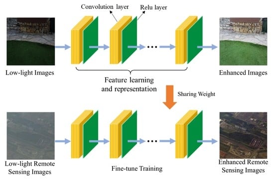
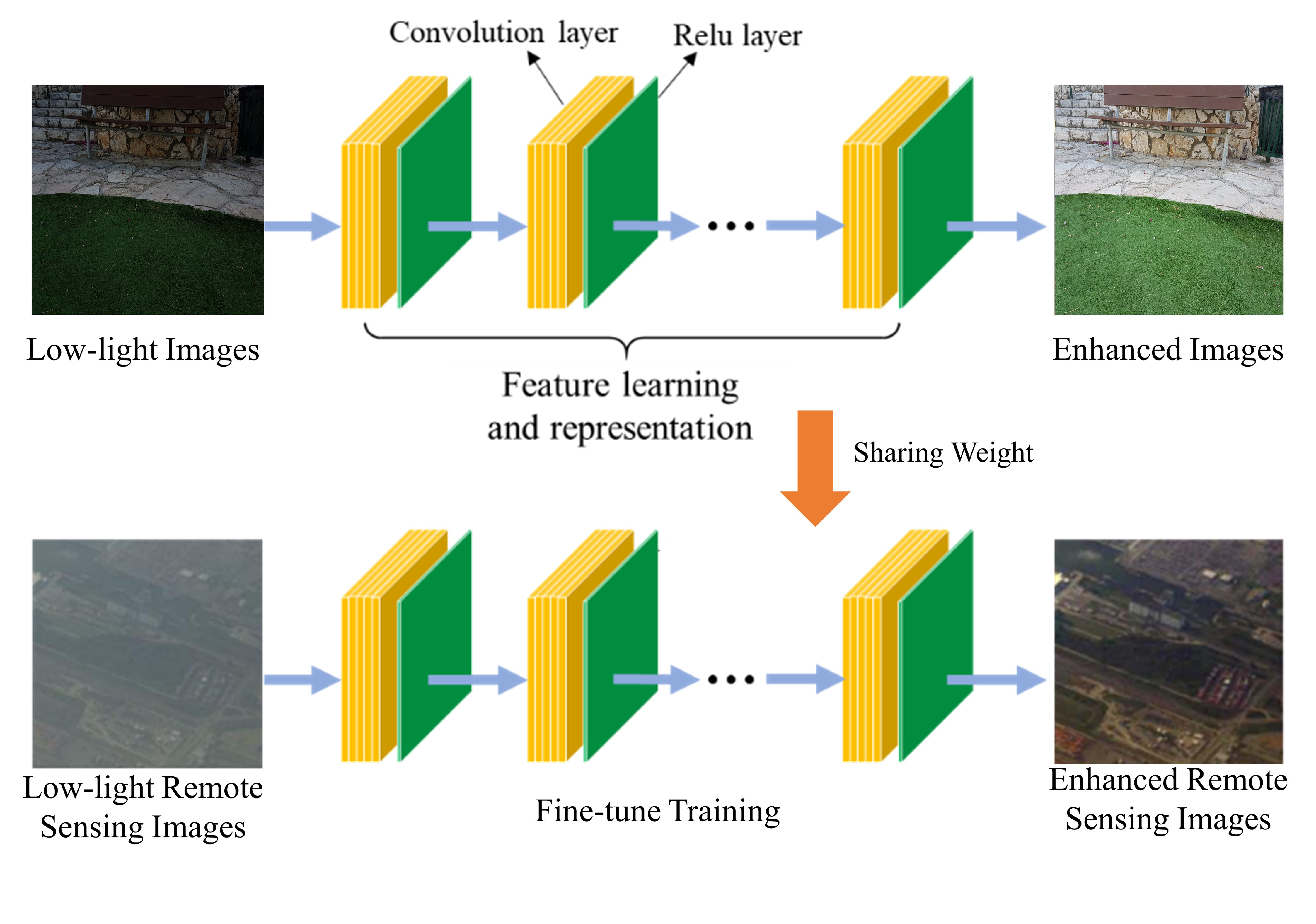
The framework of RSCNN is shown in Figure 1. A deep CNN-based model extracts the abstract features and learns the detailed information from the input low-light images. Since CNN-based models can directly process multi-channel images without color space conversion, all information of input images can be retained and the complex nonlinear relation patterns between low-light and normal-light image pairs can be well learned, thereby generating images with proper light, stronger contrast, and natural textures.
In detail, there are four main different types of components in the deep learning network, as described below.
- (1)
- Convolution layer
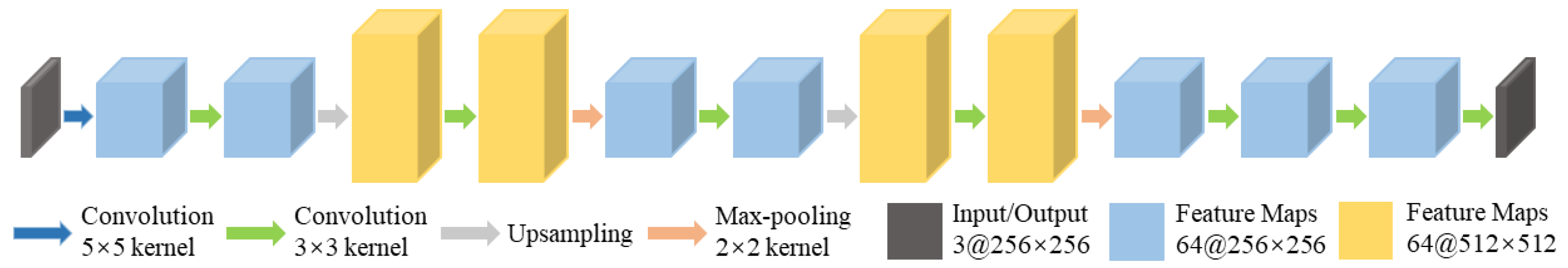
The whole network has 8 convolution layers. Each layer consists of multiple kernels, and the weights of these kernels do not change during the convolution process, i.e., there is weight sharing. With the convolution operation, RSCNN extracts the different features of the input images at different convolution levels. The output of the first CNN layer roughly depicts the location of low-level features (edges and curves) in the original image. On this basis, another convolution operation is carried out, and the output will be the activation map representing higher-level features [31]. Such features can be semicircles (a combination of curves and lines) or quadrilateral (a combination of several lines). The more convolution layers, the more complex feature activation map will be obtained. There are several parameters that need to be determined for each layer, such as the kernel size , padding , and stride . The number of kernels is the number of output feature maps. and denote the width and height of images, respectively. Thus, the size of the output feature maps can be calculated as follows:
Since we want to fix the tensor size of the input and the output for each convolution layer, we set K = 5, S = 1, and P = 2 for the first convolution layer and K = 3, S = 1, and P = 1 for the rest.
- (2)
- Activation layer
The activation layer is vital in a deep CNN because the nonlinearity of the activation layer introduces nonlinear characteristics to a system which has just undergone linear computation, gives RSCNN a stronger representational power, and avoids the occurrence of gradient saturation during training. We adopt rectified linear unit (ReLU) for its advancement in improving the training speed of RSCNN without obvious changes in accuracy. The activation layer is applied over the output of the previous layer.
Every value obtained from upper stream convolution layer should be activated by ReLU before it is input into the downstream convolution layer.
- (3)
- Upsampling operation
Inspired by the CNN for super resolution methods [32,33,34], in the RSCNN, we adopt bilinear interpolation to magnify the image by two times for a better receptive field and then add another CNN layer after that in order to learn more complex features with different scales. We use Bicubic as the interpolation method in this operation to help preserve clearer edges [35].
- (4)
- Max-pooling operation
We adopt the pooling operation in RSCNN with two purposes: Firstly, the pooling operation is helpful to reduce the number of parameters and to resize the image to the original patch image size, decreasing the training cost by a meaningful extent. Secondly, the pooling operation can cut down the possibility of overfitting, helpful to suppress noise.
In RSCNN, we set the kernel size to 2 for each max-pooling operation.
2.2. Loss Function
A combination of the SSIM loss function and the L1 loss function is adopted in RSCNN. The L1 loss function, noted as , is given as Equation (3).
where p and P represent the index of the pixel and the patch, respectively. o(p) and e(p) represent the values of the pixels in the processed patch and target ones, respectively. L1 loss can preserve pixel-wise relations between the target images and the enhanced ones of every training pair, helping enhanced images have similar light intensity to the target one. However, it gives less consideration to the overall structure of the whole image, resulting in a lack of textural details.
Additionally, low-light capture usually causes structural distortions such as blurs and artifacts, which is visually salient but cannot be well handled by pixel-wise loss functions such as the mean squared error.
The loss function, however, is helpful under this situation. The value for patch P is defined as Equation (4).
where is the original normal-light image, is the enhanced one, and are the respective pixel value averages, and are the respective variances, is the covariance, and and are the constants to prevent the denominator from being zero. A larger is means better quality of the processed images. Therefore, is defined as .
For L, we combine and as Equation (5).
The value of p is set to 0.1 in L. The training target is to minimize L.
2.3. Training
- (1)
- Datasets
There are two datasets that are used in this work: the DeepISP dataset [36] and the UCMerced dataset [37]. Their descriptions are as follows.
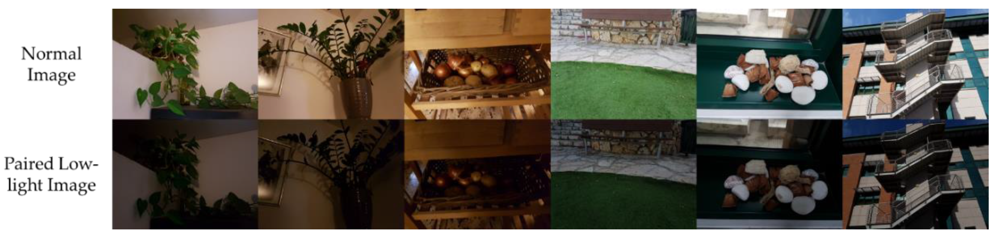
DeepISP: A total of 110 pairs of normal exposure and low-light exposure images are included, 77 for training and 33 for testing. The scenes captured include indoor and outdoor images, and sun light and artificial light with a Samsung S7 rear camera. The image pairs are almost the same, except that the low-light one has a 1/4 of the exposure time of the normal one. The resolution of each image is 3024 × 4032. Original images are divided into patches with sizes of 256 × 256. Figure 2 illustrates the representative images of every type. This dataset is named Dataset1.
UCMerced: It is composed of 21 types of land use images secondarily processed based on United States Geological Survey (USGS) National Map with a pixel resolution of one foot. Each category has 100 images of 256 × 256 pixels. Figure 3 shows some representative images of UCMerced datasets. This dataset is named Dataset2.
As far as we know, there is no specific open dataset for low-light remote-sensing image enhancement training. With respect to this dilemma, a set of natural low-light and normal-light image pairs generated from an ordinary image dataset, that is Dataset1 in this paper, is adopted for the pretrained training.
Then, because the light source angle and camera angle of remote-sensing imaging equipment have their own obvious characteristics compared with natural images, it is not proper to directly apply a model that was trained using natural image pairs to remote-sensing images. Therefore, a fine-tuning process is indispensable. First, we choose “dense residential” images from the UCMerced dataset because, compared with other categories, these images have more diverse features, richer textures, more complex shadows, and blurrier boundaries. These complex conditions make low-light images more difficult to enhance. Then, we follow the methods of [19,29] to set the original image as the ground truth and use the degradation method to generate the corresponding low-light image. A pair of low-light images and the corresponding one is used as the input and label for RSCNN training and testing. A random gamma adjustment is used to simulate the low-light images. The parameter gamma is randomly set in the range of (2, 5), enabling RSCNN to adaptively enhance the image and to have better generalization. Finally, a total of 100 pairs of normal exposure and low-light exposure images is used. They are split into 80 pairs for training and 20 pairs for testing, respectively. This dataset is named Dataset2.
- (2)
- Evaluation criteria
Since SSIM has already been described, here, we briefly describe the PSNR evaluator as follows.
where is the normal-light image and is the enhanced one generated from the low-light image. represents the maximum signal value that exists in . The higher the PSNR, the better RSCNN performs.
According Equation (6), we can see that PSNR is a variant of mean squared error (MSE). It is a pixel-wise full-reference quality metric, computed by averaging the squared intensity differences of the enhanced result and reference image pixels [11]. It is easy to calculate and has clear physical meanings but is not sensitive to the change in image structure and is not completely in accordance with human visual characteristics. SSIM makes up for PSNR. According to Equation (4), SSIM puts focus on image structure similarity and measures the image similarity from brightness (), contrast (), and structure (). PSNR and SSIM are widely used to evaluate the performance of low-light image-processing methods [22,24,26,39,40] and remote-sensing image-processing methods [20,41,42]. With the help of PSNR and SSIM, we can effectively evaluate the color retention and structural differences between enhanced images and reference images.
Furthermore, we adopt CIEDE2000 as the evaluation criteria. It is a color difference equation based on CIE’s lab color space (CIELAB) and is published by the International Commission on Illumination (CIE) in Publication 142-2001. It can help us evaluate the degree of color difference between the ground-truth image and the enhanced image. The smaller CIEDE2000 is, the closer the result image is to the ground-truth image. We use the “imcolordiff” function in Matlab 2020b for CIEDE2000. It is based on [43].
2.4. Implementation Details
There are 3 kinds of CONVs: 1-D-CNNs, 2-D-CNNs, and 3-D-CNNs. Since we want to treat the input image patches as a whole with spatial information, we choose a 2-D-CNN as the CONV in our network [44]. The configuration of each convolution layer is shown in Figure 1. The weights of each CONV layer are initialized using kaiming_normal [45].
During training, the patch-size is set to 256 × 256 and the depth of the whole network is 8. In addition, Adam optimization is adopted with a weight decay of 0.0001. The base learning rate is 0.001, and the batch size is 8. Our model is trained using PyTorch.
2.5. Baselines
Ten different methods, which are shown in Table 1, are compared with our proposed method.
As observed, different types of models are considered. The models that are used apply the default settings suggested by the authors.
3. Results and Discussion
3.1. Comparison Results on Dataset1
The experiment is first carried out on Dataset1, and 9 different methods are compared with RSCNN. Detailed results are presented in Table 2. In the experimental results, the SSIMs of DHE and CLAHE are significantly improved compared to ordinary HE, and the PSNR result of DHE is the best. Compared with the histogram equalization algorithms, the Retinex algorithms achieve better indicator results. Among them, the SSIM of the MSRCR method is about 12% higher than that of DHE but, because its adjustment method is not global pixel-wise, the PSNR is 8% lower than that of DHE. With respect to LIME and BIMEF, compared with the traditional histogram method and the Retinex method, it has a better effect in maintaining the overall visual characteristics and pixel-wise results. DWT-SVD is often used for low-light remote-sensing image enhancement. The results of DWT-SVD are similar to the enhancement algorithms based on luminance estimation.
Obviously, from the perspective of quantitative analysis indicators, the results of RSCNN have better results than various traditional low-light enhancement algorithms and can be applied to low-light remote-sensing image enhancement tasks. For example, the SSIM of the RSCNN is 0.825, which is 0.2 higher than that of the widely used DWT-SVD algorithm. As for the PSNR, our method achieved 28.123 dB, which is much better than those of all these baselines since their PSNRs are lower than 20 dB.
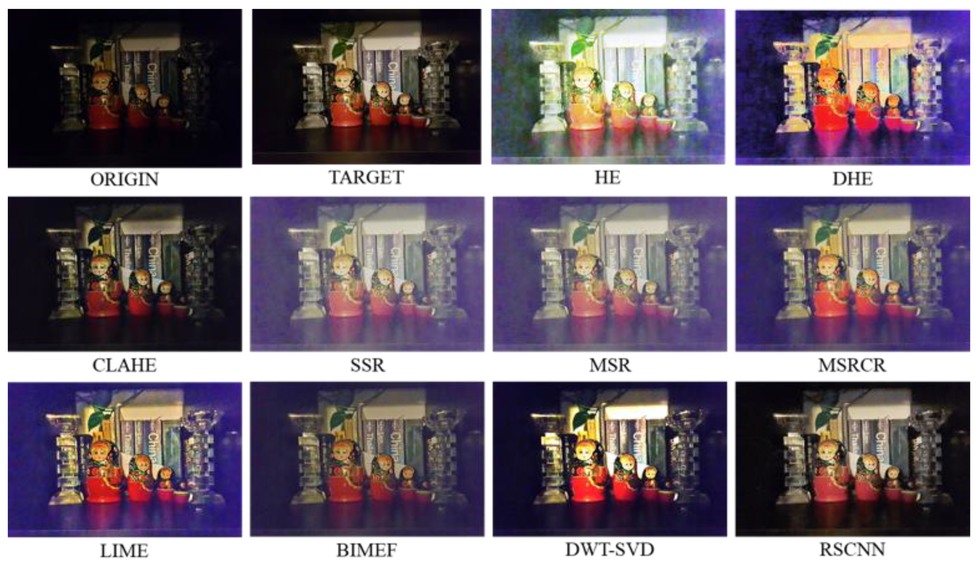
As shown in Figure 4, in general, all the methods are able to obtain brighter images with stronger contrast. However, the results of many methods are not sufficient and satisfactory. For example, HE-based methods such as HE, DHE, and CLAHE can inappropriately enhance the dark background (too bright or too dark) and can cause color distortions. SR-based methods (i.e., SSR, MSR, and MSRCR) and LIME are able to appropriately enhance the dark background, but the color distortions are also very severe and the background is enhanced to be blue instead of actual dark.
As for color distortion, CLAHE, DWT-SVD, and RSCNN work relatively better, and the backgrounds of the enhanced images are very close to those of the target images. However, DWT-SVD and CLAHE suffer from over-enhanced and insufficient brightness, respectively, in the high-contrast region, which is not as natural as that of our proposed RSCNN. In addition, the HE and DHE enhanced images have significant noise, and SSR and MSR generate images that appear to be covered by haze. Meanwhile, the images that are enhanced by our proposed method are sharper and have better brightness than those of other methods thanks to its powerful feature extraction ability and learning ability.
3.2. Comparison Results on Dataset2
To evaluate the performance of RSCNN on the low-light remote-sensing images, we fine-tuned the trained model and tested it using Dataset2. The results are presented in Table 3. In addition, Figure 5 shows the visual results to compare the proposed method with other methods. In remote-sensing image enhancement, preserving accurate textural and structural information is very important for many applications including scene classification [46] and object detection [47]. In addition, obtaining images with natural colors is also of great significance for visual discrimination and further analysis.
As we can see from Table 3, the comparison results indicate that RSCNN has the best performance compared to all other low-light image enhancement methods. Specifically, the SSIM, PSNR, and CIEDE2000 of our method are 0.791, 20.936 dB, and 19.496, respectively. To comprehensively support the qualitative conclusions of the superiority of RSCNN, visual comparison and analysis are also needed.
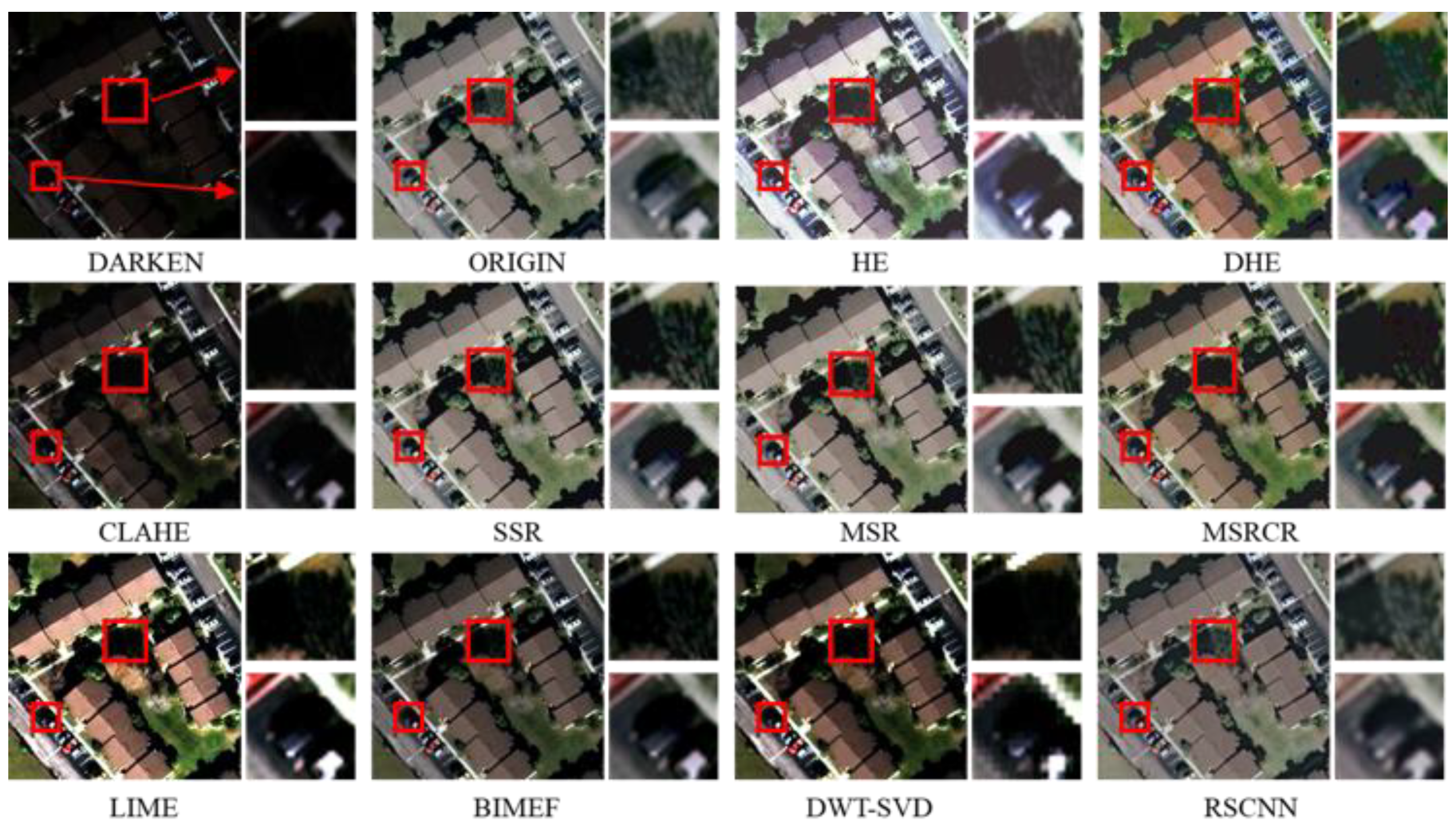
Figure 5 shows the image-enhancement results obtained using different methods for qualitative comparison. In addition, the patches in the two red boxes are enlarged to show detailed information. As shown in Figure 5, all the methods obtain images with stronger contrast and brightness. However, the results of CLAHE, BIMEF, and DWT-SVD may not be sufficiently enhanced since the brightness is still somewhat dim. In addition, different methods have different characteristics, resulting in different effects.
For example, in terms of the image colors, the buildings obtained by HE, DHE, and LIME are enhanced to be different colors, which are far from the standard natural images. The estimated images generated by SSR, MSR, and RSCNN are much better than other methods. As for detailed information such as edges and textures in dark regions, HE, DHE, and LIME are able to obtain clear cars. However, several other methods cannot accurately replicate the detailed information. For example, the textures of cars that are generated by CLAHE, BIMEF, and DWT-SVD are very dark and blurred, which make it hard to figure out the shape, and even the trees cannot be visually recognized since they are nearly black. Additionally, although the results from MSR and SSR are free of apparent color distortion, they suffer from apparent grid-like veins, which can be avoided by using our method. As a whole, the visual effects of the RSCNN are the closest to the original image in both color and texture. For instance, RSCNN preserves the details of trees and cars and enhances remote-sensing image with little information loss, thus making the images more realistic than those of other methods.
4. Conclusions
An end-to-end RSCNN model is proposed in this paper to get brighter images from degraded low-light images and is applied to remote-sensing images. A CNN architecture is used to achieve end-to-end enhancement for low-light remote-sensing images. The usampling and downsampling operators are designed to learn deep features from different scales. In this way, the enhanced images can have more detailed features. Compared to other traditional methods, our result achieves more natural results with more realistic textures and vivid details while revealing the edge features and structural features as much as possible. It can help a lot with subsequent high-level remote-sensing image information-discovery tasks.
Author Contributions
Conceptualization, methodology, and original draft preparation, L.H. and M.Q.; investigation, review, editing, and supervision, F.Z.; project administration snf funding acquisition, F.Z., Z.D. and R.L. All authors have read and agreed to the published version of the manuscript.
Funding
This research was funded by the National Key R&D Program of China (2019YFE0127400) and the National Natural Science Foundation of China (41671391, 41922043, and 41871287).
Conflicts of Interest
The authors declare no conflict of interest.
References
- Yang, J.; Gong, P.; Fu, R.; Zhang, M.; Chen, J.; Liang, S. Dickinson, R. The role of satellite remote sensing in climate change studies. Nat. Clim. Chang. 2013, 3, 875–883. [Google Scholar] [CrossRef]
- Gastellu-Etchegorry, J.P. 3D modeling of satellite spectral images, radiation budget and energy budget of urban landscapes. Meteorol. Atmos. Phys. 2008, 102, 187–207. [Google Scholar] [CrossRef] [Green Version]
- Jones, M.O.; Jones, L.A.; Kimball, J.S.; McDonald, K.C. Satellite passive microwave remote sensing for monitoring global land surface phenology. Remote Sens. Environ. 2011, 115, 1102–1114. [Google Scholar] [CrossRef]
- Liu, C.; Cheng, I.; Zhang, Y.; Basu, A. Enhancement of low visibility aerial images using histogram truncation and an explicit Retinex representation for balancing contrast and color consistency. ISPRS J. Photogramm. Remote Sens. 2017, 128, 16–26. [Google Scholar] [CrossRef]
- Zollini, S.; Alicandro, M.; Cuevas-González, M.; Baiocchi, V.; Dominici, D.; Buscema, P.M. Shoreline extraction based on an active connection matrix (ACM) image enhancement strategy. J. Mar. Sci. Eng. 2020, 8, 9. [Google Scholar] [CrossRef] [Green Version]
- Dominici, D.; Zollini, S.; Alicandro, M.; della Torre, F.; Buscema, P.M.; Baiocchi, V. High resolution satellite images for instantaneous shoreline extraction using new enhancement algorithms. Geosciences 2019, 9, 123. [Google Scholar] [CrossRef] [Green Version]
- Gonzalez, R.C.; Woods, R.E.; Masters, B.R. Digital Image Processing, Third Edition. J. Biomed. Opt. 2009, 14, 029901. [Google Scholar] [CrossRef]
- Abdullah-Al-Wadud, M.; Kabir, M.; Dewan, M.A.; Chae, O. A Dynamic Histogram Equalization for Image Contrast Enhancement. IEEE Trans. Consum. Electron. 2007, 53, 593–600. [Google Scholar] [CrossRef]
- Ibrahim, H.; Kong, N.S.P. Brightness preserving dynamic histogram equalization for image contrast enhancement. IEEE Trans. Consum. Electron. 2007, 53, 1752–1758. [Google Scholar] [CrossRef]
- Asha, S.; Sreenivasulu, G. Satellite Image Enhancement Using Contrast Limited Adaptive Histogram Equalization. Int. J. Sci. Res. Sci. Eng. Technol. 2018, 4, 1070–1075. [Google Scholar]
- Zhou, W. Image quality assessment: From error measurement to structural similarity. IEEE Trans. Image Process. 2004, 13, 600–613. [Google Scholar]
- Tao, L.; Zhu, C.; Song, J.; Lu, T.; Jia, H.; Xie, X. Low-light image enhancement using CNN and bright channel prior. In Proceedings of the IEEE International Conference on Image Processing (ICIP), Beijing, China, 17–20 September 2017; pp. 3215–3219. [Google Scholar]
- Jobson, D.J.; Rahman, Z.U.; Woodell, G.A. Properties and performance of a center/surround retinex. IEEE Trans. Image Process. 1997, 6, 451–462. [Google Scholar] [CrossRef] [PubMed]
- Rahman, Z.; Jobson, D.J.; Woodell, G.A. Multi-scale retinex for color image enhancement. IEEE Int. Conf. Image Process. 1996, 3, 1003–1006. [Google Scholar]
- Jobson, D.J.; Rahman, Z.U.; Woodell, G.A. A multiscale retinex for bridging the gap between color images and the human observation of scenes. IEEE Trans. Image Process. 1997, 6, 965–976. [Google Scholar] [CrossRef] [PubMed] [Green Version]
- Guo, X.; Li, Y.; Ling, H. LIME: Low-Light Image Enhancement via Illumination Map Estimation. IEEE Trans. Image Process. 2017, 26, 982–993. [Google Scholar] [CrossRef] [PubMed]
- Ying, Z.; Li, G.; Gao, W. A Bio-Inspired Multi-Exposure Fusion Framework for Low-light Image Enhancement. arXiv 2017, arXiv:1711.00591. [Google Scholar]
- Lee, C.-H.; Shih, J.-L.; Lien, C.-C.; Han, C.-C. Adaptive multiscale retinex for image contrast enhancement. In Proceedings of the International Conference on Signal-Image Technology & Internet-Based Systems, Kyoto, Japan, 2–5 December 2013; pp. 43–50. [Google Scholar]
- Ying, Z.; Li, G.; Ren, Y.; Wang, R.; Wang, W. A new image contrast enhancement algorithm using exposure fusion framework. In International Conference on Computer Analysis of Images and Patterns; Springer: Cham, Germany, 2017; pp. 36–46. [Google Scholar]
- Bhandari, A.K.; Soni, V.; Kumar, A.; Singh, G.K. Cuckoo search algorithm based satellite image contrast and brightness enhancement using DWT–SVD. ISA Trans. 2014, 53, 1286–1296. [Google Scholar] [CrossRef]
- Demirel, H.; Ozcinar, C.; Anbarjafari, G. Satellite image contrast enhancement using discrete wavelet transform and singular value decomposition. IEEE Geosci. Remote Sens. Lett. 2010, 7, 333–337. [Google Scholar] [CrossRef]
- Li, C.; Guo, J.; Porikli, F.; Pang, Y. LightenNet: A Convolutional Neural Network for weakly illuminated image enhancement. Pattern Recognit. Lett. 2018, 104, 15–22. [Google Scholar] [CrossRef]
- Wei, C.; Wang, W.; Yang, W.; Liu, J. Deep Retinex Decomposition for Low-Light Enhancement. arXiv 2018, arXiv:1808.04560. [Google Scholar]
- Lore, K.G.; Akintayo, A.; Sarkar, S. LLNet: A deep autoencoder approach to natural low-light image enhancement. Pattern Recognit. 2017, 61, 650–662. [Google Scholar] [CrossRef] [Green Version]
- Xie, J.; Xu, L.; Chen, E. Image denoising and inpainting with deep neural networks. Adv. Neural Inf. Process. Syst. 2012, 1, 341–349. [Google Scholar]
- Tao, L.; Zhu, C.; Xiang, G.; Li, Y.; Jia, H.; Xie, X. LLCNN: A convolutional neural network for low-light image enhancement. In Proceedings of the IEEE Visual Communications and Image Processing (VCIP), St. Petersburg, FL, USA, 10–13 December 2017; pp. 1–4. [Google Scholar]
- Lv, F.; Lu, F.; Wu, J.; Lim, C. MBLLEN: Low-light Image/Video Enhancement Using CNNs. In Proceedings of the British Machine Vision Conference (BMVC), Newcastle, UK, 3–6 September 2018; pp. 1–13. [Google Scholar]
- Chen, C.; Chen, Q.; Xu, J.; Koltun, V. Learning to see in the dark. arXiv 2018, arXiv:1805.01934. [Google Scholar]
- Fu, X.; Wang, J.; Zeng, D.; Huang, Y.; Ding, X. Remote Sensing Image Enhancement Using Regularized-Histogram Equalization and DCT. IEEE Geosci. Remote Sens. Lett. 2015, 12, 2301–2305. [Google Scholar] [CrossRef]
- Lee, E.; Kim, S.; Kang, W.; Seo, D.; Paik, J. Contrast enhancement using dominant brightness level analysis and adaptive intensity transformation for remote sensing images. IEEE Geosci. Remote Sens. Lett. 2013, 10, 62–66. [Google Scholar] [CrossRef]
- Zeiler, M.D.; Fergus, R. Visualizing and Understanding Convolutional Networks. In Proceedings of the European Conference on Computer Vision (ECCV), Zurich, Switzerland, 6–12 September 2014; Springer: Cham, Switzerland, 2014; pp. 818–833. [Google Scholar]
- Lai, W.S.; Huang, J.B.; Ahuja, N.; Yang, M.H. Deep laplacian pyramid networks for fast and accurate super-resolution. In Proceedings of the IEEE Conference on Computer Vision and Pattern Recognition (CVPR), Honolulu, HI, USA, 21–26 July 2017; pp. 5835–5843. [Google Scholar]
- Zhao, Y.; Li, G.; Xie, W.; Jia, W.; Min, H.; Liu, X. GUN: Gradual Upsampling Network for Single Image Super-Resolution. IEEE Access 2018, 6, 39363–39374. [Google Scholar] [CrossRef]
- Wang, Y.; Wang, L.; Wang, H.; Li, P. End-to-End Image Super-Resolution via Deep and Shallow Convolutional Networks. IEEE Access 2019, 7, 31959–31970. [Google Scholar] [CrossRef]
- Joshi, S.H.; Marquina, A.L.; Osher, S.J.; Dinov, I.; Toga, A.W.; van Horn, J.D. Fast edge-filtered image upsampling. In Proceedings of the 18th IEEE International Conference on Image Processing (ICIP), Brussels, Belgium, 11–14 September 2011; pp. 1165–1168. [Google Scholar]
- Schwartz, E.; Giryes, R.; Bronstein, A.M. DeepISP: Toward learning an end-to-end image processing pipeline. IEEE Trans. Image Process. 2019, 28, 912–923. [Google Scholar] [CrossRef] [Green Version]
- Yang, Y.; Newsam, S. Bag-of-visual-words and spatial extensions for land-use classification. In Proceedings of the 18th SIGSPATIAL International Conference on Advances in Geographic Information Systems, San Jose, CA, USA, 2–5 November 2010; pp. 270–279. [Google Scholar]
- Luo, M.R.; Cui, G.; Rigg, B. The development of the CIE 2000 colour-difference formula: CIEDE2000. Color. Res. Appl. 2001, 26, 340–350. [Google Scholar] [CrossRef]
- Dong, C.; Loy, C.C.; He, K.; Tang, X. Image Super-Resolution Using Deep Convolutional Networks. IEEE Trans. Pattern Anal. Mach. Intell. 2016, 38, 295–307. [Google Scholar] [CrossRef] [Green Version]
- Shen, L.; Yue, Z.; Feng, F.; Chen, Q.; Liu, S.; Ma, J. MSR-net:Low-light Image Enhancement Using Deep Convolutional Network. arXiv 2017, arXiv:1711.02488. [Google Scholar]
- Kundeti, N.M.; Kalluri, H.K.; Krishna, S.V.R. Image enhancement using DT-CWT based cycle spinning methodology. In Proceedings of the IEEE International Conference on Computational Intelligence and Computing Research (ICCIC), Madurai, India, 26–28 December 2013; pp. 185–188. [Google Scholar]
- Rasti, P.; Lüsi, I.; Demirel, H.; Kiefer, R.; Anbarjafari, G. Wavelet transform based new interpolation technique for satellite image resolution enhancement. In Proceedings of the IEEE International Conference on Aerospace Electronics and Remote Sensing Technology, Yogyakarta, Indonesia, 13–14 November 2014; pp. 185–188. [Google Scholar]
- Sharma, G.; Wu, W.; Dalal, E.N. The CIEDE2000 color-difference formula: Implementation notes, supplementary test data, and mathematical observations. Color. Res. Appl. 2005, 30, 21–30. [Google Scholar] [CrossRef]
- Haut, J.M.; Fernandez-Beltran, R.; Paoletti, M.E.; Plaza, J.; Plaza, A.; Pla, F. A new deep generative network for unsupervised remote sensing single-image super-resolution. IEEE Trans. Geosci. Remote Sens. 2018, 56, 6792–6810. [Google Scholar] [CrossRef]
- He, K.; Zhang, X.; Ren, S.; Sun, J. Delving deep into rectifiers: Surpassing human-level performance on imagenet classification. In Proceedings of the IEEE International Conference on Computer Vision (ICCV), Santiago, Chile, 7–13 December 2015; pp. 1026–1034. [Google Scholar]
- Hu, F.; Xia, G.S.; Hu, J.; Zhang, L. Transferring deep convolutional neural networks for the scene classification of high-resolution remote sensing imagery. Remote Sens. 2015, 7, 14680–14707. [Google Scholar] [CrossRef] [Green Version]
- Cheng, G.; Zhou, P.; Han, J. Learning rotation-invariant convolutional neural networks for object detection in VHR optical remote sensing images. IEEE Trans. Geosci. Remote Sens. 2016, 54, 7405–7415. [Google Scholar] [CrossRef]
Figure 1.
The framework of the RSCNN.

Figure 2.
The representative images of DeepISP of every type [36].
Figure 2.
The representative images of DeepISP of every type [36].

Figure 3.
The representative images of UCMerced for every type [37].
Figure 3.
The representative images of UCMerced for every type [37].

Figure 4.
Image-enhancement results with different methods, including Histogram Equalization (HE), Dynamic Histogram Equalization (DHE), Contrast Constrained Adaptive Histogram Equalization (CLAHE), Single-scale Retinex (SSR), Multi-scale Retinex (MSR), Multi-scale Retinex with Color Restoration (MSRCR), Low-light Image Enhancement (LIME), Bio-Inspired Multi-Exposure Fusion (BIMEF), Discrete Wavelet Transform and Singular Value Decomposition (DWT-SVD), and RSCNN.

Figure 5.
Results of remote-sensing image enhancement with different methods, including HE, DHE, CLAHE, SSR, MSR, MSRCR, LIME, BIMEF, DWT-SVD, and RSCNN.
Figure 5.
Results of remote-sensing image enhancement with different methods, including HE, DHE, CLAHE, SSR, MSR, MSRCR, LIME, BIMEF, DWT-SVD, and RSCNN.


Table 1.
Methods for comparison experiments.
| Methods | Abbreviation | Type | |
|---|---|---|---|
| 1 | Histogram Equalization [7] | HE | Histogram |
| 2 | Dynamic Histogram Equalization (DHE) [8] | DHE | Histogram |
| 3 | Contrast Limited Adaptive Histogram Equalization [10] | CLAHE | Histogram |
| 4 | Single-scale Retinex [13] | SSR | Retinex |
| 5 | Multi-scale Retinex [14] | MSR | Retinex |
| 6 | Multi-Scale Retinex with Color Restoration [15] | MSRCR | Retinex |
| 7 | Low-light image enhancement method [16] | LIME | Illumination map estimation and Retinex |
| 8 | Bio-Inspired Multi-Exposure Fusion Framework for Low-light Image Enhancement [17] | BIMEF | Illumination map estimation and camera response model |
| 9 | Discrete Wavelet Transform and Singular Value Decomposition [21] | DWT-SVD | Frequency domain |
Table 2.
Average structural similarity indexes (SSIMs) and peak signal-to-noise ratios (PSNRs) of the testing results after pretraining.
Table 2.
Average structural similarity indexes (SSIMs) and peak signal-to-noise ratios (PSNRs) of the testing results after pretraining.
| SSIM | PSNR | |
|---|---|---|
| HE | 0.482 | 16.774 |
| DHE | 0.546 | 18.080 |
| CLAHE | 0.548 | 14.192 |
| SSR | 0.570 | 14.529 |
| MSR | 0.585 | 13.959 |
| MSRCR | 0.610 | 16.582 |
| LIME | 0.464 | 17.152 |
| BIMEF | 0.632 | 17.646 |
| DWT-SVD | 0.617 | 17.806 |
| RSCNN | 0.825 | 28.194 |
Table 3.
Average SSIMs and PSNRs of the test results after fine-tuning.
| SSIM | PSNR | CIEDE2000 | |
|---|---|---|---|
| HE | 0.730 | 15.905 | 67.628 |
| DHE | 0.706 | 16.357 | 52.272 |
| CLAHE | 0.546 | 13.857 | 70.600 |
| SSR | 0.711 | 20.424 | 30.972 |
| MSR | 0.751 | 20.610 | 28.586 |
| MSRCR | 0.680 | 19.088 | 38.212 |
| LIME | 0.630 | 15.074 | 60.154 |
| BIMEF | 0.728 | 16.302 | 50.697 |
| DWT-SVD | 0.564 | 13.989 | 76.490 |
| RSCNN | 0.852 | 21.691 | 19.496 |
Publisher’s Note: MDPI stays neutral with regard to jurisdictional claims in published maps and institutional affiliations. |
© 2020 by the authors. Licensee MDPI, Basel, Switzerland. This article is an open access article distributed under the terms and conditions of the Creative Commons Attribution (CC BY) license (http://creativecommons.org/licenses/by/4.0/).
Share and Cite
MDPI and ACS Style
Hu, L.; Qin, M.; Zhang, F.; Du, Z.; Liu, R. RSCNN: A CNN-Based Method to Enhance Low-Light Remote-Sensing Images. Remote Sens. 2021, 13, 62. https://0-doi-org.brum.beds.ac.uk/10.3390/rs13010062
AMA Style
Hu L, Qin M, Zhang F, Du Z, Liu R. RSCNN: A CNN-Based Method to Enhance Low-Light Remote-Sensing Images. Remote Sensing. 2021; 13(1):62. https://0-doi-org.brum.beds.ac.uk/10.3390/rs13010062
Chicago/Turabian StyleHu, Linshu, Mengjiao Qin, Feng Zhang, Zhenhong Du, and Renyi Liu. 2021. "RSCNN: A CNN-Based Method to Enhance Low-Light Remote-Sensing Images" Remote Sensing 13, no. 1: 62. https://0-doi-org.brum.beds.ac.uk/10.3390/rs13010062
Note that from the first issue of 2016, this journal uses article numbers instead of page numbers. See further details here.