
Assessing Freshwater Changes over Southern and Central Africa (2002–2017)


1
Department of Geoinformatics & Surveying, University of Uyo, Uyo P.M.B. 1017, Nigeria
2
Australian Rivers Institute, Griffith University, Nathan, QLD 4111, Australia
3
School of Environment & Science, Griffith University, Nathan, QLD 4111, Australia
*
Author to whom correspondence should be addressed.
Remote Sens. 2021, 13(13), 2543; https://0-doi-org.brum.beds.ac.uk/10.3390/rs13132543
Submission received: 1 June 2021
/
Revised: 19 June 2021
/
Accepted: 25 June 2021
/
Published: 29 June 2021
(This article belongs to the Special Issue Remote Sensing of Floodplain Rivers and Freshwater Ecosystems)
Abstract
:In large freshwater river basins across the globe, the composite influences of large-scale climatic processes and human activities (e.g., deforestation) on hydrological processes have been studied. However, the knowledge of these processes in this era of the Anthropocene in the understudied hydrologically pristine South Central African (SCA) region is limited. This study employs satellite observations of evapotranspiration (ET), precipitation and freshwater between 2002 and 2017 to explore the hydrological patterns of this region, which play a crucial role in global climatology. Multivariate methods, including the rotated principal component analysis (rPCA) were used to assess the relationship of terrestrial water storage (TWS) in response to climatic units (precipitation and ET). The use of the rPCA technique in assessing changes in TWS is warranted to provide more information on hydrological changes that are usually obscured by other dominant naturally-driven fluxes. Results show a low trend in vegetation transpiration due to deforestation around the Congo basin. Overall, the Congo (r2 = 76%) and Orange (r2 = 72%) River basins maintained an above-average consistency between precipitation and TWS throughout the study region and period. Consistent loss in freshwater is observed in the Zambezi (−9.9 ± 2.6 mm/year) and Okavango (−9.1 ± 2.5 mm/year) basins from 2002 to 2008. The Limpopo River basin is observed to have a 6% below average reduction in rainfall rates which contributed to its consistent loss in freshwater (−4.6 ± 3.2 mm/year) from 2006 to 2012.Using multi-linear regression and correlation analysis we show that ET contributes to the variability and distribution of TWS in the region. The relationship of ET with TWS (r = 0.5) and rainfall (r = 0.8) over SCA provides insight into the role of ET in regulating fluxes and the mechanisms that drive precipitation in the region. The moderate ET–TWS relationship also shows the effect of climate and anthropogenic influence in their interactions.
Keywords:
freshwater; GRACE; TWS; precipitation; evapotranspiration; Africa; hydrology; climate change1. Introduction
Terrestrial water storage (TWS) is a function of changes in the earth’s gravity fields. Its relation to hydrological applications is characterized by the sum of water stored underground, in the soil, as snow, over the land surface, and canopy. The changes in any of the above components remain one of the most critical elements in the balance of the hydrological cycle. Monitoring the changes that occur within these TWS components is an important hydrological exercise, as it helps in determining the cause of climate change, thus making a cogent recommendation as to the required environmental response necessary to mitigate potential climatic hazards at the basin or regional scale. With the advent of satellite remote sensing and altimetry, extensive data collection and observation that have been recorded in hydrology, especially in the monitoring of water storage and fluxes in a changing world, thus enabling a universal evaluation that spans political boundaries [1,2,3].
An important intention of this study is to understand the hydrological response of the South Central African (SCA) region to climatic conditions. Amidst other factors that contribute to climate change, the study focuses on two notable water cycle variants; evapotranspiration (ET) and precipitation. The net-zero water cycle is achieved majorly as a result of these two factors. Spatial and temporal variability in rainfall amount and evapotranspiration indexes as a result of global climate change is posing a serious danger to water resources management, food security, rain-fed agriculture, and poverty reduction, especially in developing countries such asthe SCA region. Therefore, understanding the variability, magnitude, patterns, and drivers of precipitation and evapotranspiration is crucial for studying the climate systems of the SCA region. Following substantial environmental shifts such as deforestation, increased temperature patterns due to anthropogenic climate change, fluctuations in precipitation patterns amongst others being reported around the SCA region [4,5,6,7,8,9,10,11,12,13], a potential climatic backlash is inevitable. We therefore attempt to comprehend the region’s response to these conditions through a short-term trend analysis between 2002 and 2017 to make informed decisions about managing the expected regional climatic shifts.
Southern and Central Africa is a region of strong climatic hotspots that play key roles in global climate. For instance, the Zambezi, Orange, Okavango and Limpopo basins in Southern Africa discharge approximately 400 cubic km of water every year, while the Congo basin’s rainfall climatology in Central Africa overshadows global tropical rainfall during transition seasons, thereby contributing to the global climatic impacts, as well as water resources and socio-economic changes [14,15,16,17,18]. Additionally, an estimated 25% to 40% of ET from the Congo River basin is recycled as local rainfall, and model simulations show that variations in ET rates within the basin area affect the moisture cycling phase across the African continent [4]. The temporal evaluation by Mohammed and David (2019) [19] between 2002 and 2017 showed a significant variation in TWS over the Congo basin in Central Africa, which extends to the southwestern part of Sudan. Furthermore, intense water deficit anomalies in Central Africa between 2005 and 2007 [14,20], and the recent progressive negative trend in TWS of SCA (Mohammed and David, 2019; Hua et al., 2016; Sorí et al., 2017) [10,20,21], are undoubtedly clear impacts of climate variability, as well as pointers to climate change in the Central and Southern African region.
Assessing and monitoring variations in hydrological patterns at a global scale is practically difficult with the use of insitu observations alone, especially due to the high cost of installing and maintaining station controls, as well as the existence of gaps in gauged data (Rodell et al., 2018) [22]. With the advent of satellite remote sensing in monitoring water storage and fluxes, several studies have shown how satellite observations can be used to improve understanding of globalhydrology (Burnett et al., 2020;Ahmed et al., 2019) [23,24]. The launch of the Gravity Recovery and Climate Experiment (GRACE) satellite mission made this possible, including tracking of ice-sheet and glacier ablation, monitoring of groundwater depletion, and impacts of climate change on freshwater variations (e.g., Tapley et al., 2004; Wahr et al., 1998; Rodell and Famiglietti, 1999; Swenson et al., 2006; Cazenave et al., 2010) [25,26,27,28,29].
GRACE is extensively used in the estimation of variations in TWS over African hotspots in recent times. Its use in hydro-geological investigations in the regions include, but are not limited to (i) prediction and estimation of TWS changes (Ahmed et al., 2019; Forootan et al., 2014) [24,30], (ii) evapotranspiration evaluation (López et al., 2017; Andam-Akorful et al., 2015; Burnett et al., 2020) [23,31,32], (iii) inspection of flood and drought episodes (Awange et al., 2016; Anderson et al., 2012; Ahmed et al., 2019) [33,34,35], (iv) reconciliation of the relationship between TWS changes and climatic events (Mohammed and David, 2019; Omondi et al., 2014; Ndehedehe et al., 2017, 2018; Anyah et al., 2018) [19,36,37], (v) standardization and corroboration of hydrological and land surface models (Xie et al., 2012; Pedinotti et al., 2012; Kittel et al., 2018; Grippa et al., 2011; Ahmed et al., 2016) [38,39,40,41,42], (vi) monitoring reservoirs, lakes and surface water resources (Swenson and Wahr, 2009; Hassan and Jin, 2014a, 2014b; Becker et al., 2018, 2010) [43,44,45,46,47], (vii) keeping under observation, the fluctuation rates of underground water storage (Sultan et al., 2014, 2013; Nanteza et al., 2016; Mohamed et al., 2016; Mazzoni et al., 2018; Lezzaik et al., 2018; Henry, 2011; Gonçalvès et al., 2013; Ahmed and Abdelmohsen, 2018; Abdelmohsen et al., 2019) [48,49,50,51,52,53,54,55], (viii) prediction and mapping of TWS variations (Rodell et al., 2018; Rateb et al., 2017; Ramillien et al., 2014; Ni et al., 2017; Ndehedehe et al., 2016a, 2017; Moore and Williams, 2014; Krogh et al., 2010; Hassan and Jin, 2016; Hasan et al., 2019; Guan et al., 2014; Boy et al., 2012; Ahmed et al., 2011, 2014; Ferreira et al., 2018; Crowley et al., 2006) [14,15,22,56,57,58,59,60,61,62,63,64,65,66].
The trend study carried out by Ahmed et al., (2019) [19] and Rodell et al., (2018) [22] used the breakpoint algorithm and apparent trend analysis, respectively. This breakpoint algorithm, which identifies the structural changes in the regression relationship and splits the time series into different segments, suffers from a high snapping tendency causing instability in the run-time system in the event of inexact medians [67,68]. In a bid to improve our understanding of the land water storage over SCA and to monitor the changes and hydro-geological fluctuations at the major river basins in the region, this study attempts to emphasize the recent annual and seasonal inconsistencies of the region’s TWS within the period between 2002 and 2017 by estimating the variability trends in TWS using the rotated principal component analysis. The rPCA technique is an improvement on the normal PCA technique which assesses extra elements in the reduction of the dimensionality of a dataset, as well as discovering hidden structures in the dataset. Since the rPCA technique is a non-parametric method, it can be applied todata with any distribution. Analogous to the study carried out by Ujeneva and Abiodun, (2015) [52], the rotated varimax option is implemented to distinguish spatial coherence (modes) in the temporal variability of the TWS. Its prevalence over other methods of trend analysis (breakpoint and apparent trend analysis) is due to its dedication to the varied retained variability modes, as well as the ease in correlating against them (Jolliffe et al., 2003) [69,70]. Besides academic curiosity, this work equally attempts to assess the merit of the study undertaken by Rodell et al., (2018) [22] who used the apparent trend analysis to observe a significant increase and substantial wetting trend within the SCA region between 2002 and 2016. The study also reported a negative trend along the coast of Southeastern Africa (housing the Limpopo River basin) of −12.9 ± 2.3 Gt year−1, reflecting a recent severe drought in the region (Figure 1g,h). The intended approach is based on the analysis of the relationship and existing variability between the GRACE-derived TWS changes and other relevant remote sensing datasets applied in this study. This region-based investigation attempts to quantify and assess the short-term trends in GRACE-derived TWS over SCA as well as explore the factors (natural or anthropogenic) contributing to the trend.
Therefore, with the implementation of a rotated principal component analysis (rPCA), and multiple linear regression analysis (MLRA), this study looks into inter-annual and seasonal fluctuations in TWS variations using GRACE and climate drivers over SCA, i.e., precipitation and evapotranspiration patterns in the region. This study specifically seeks to (i) distinguish trends and TWS variability hotspots in relation to rainfall and ETa over SCA (ii) improve understanding ofthe seasonal cycle of TWS and attempt to make future predictions of hydrological state and patterns (iii) study the rate of evapotranspiration as a result of temperature fluctuations as well as its relationship to TWS variability.
This study, however, differs from those of Ndehedehe et al. (2016a) [14] and Krough et al. (2010) [60] by (i) utilizing ETa in making predictions of climate variations (iii) correlating changes in GRACE-derived TWS with changes in climate derived output (e.g., TWS vs. ETa).
The remainder of this study is segmented as follows; Section 2 provides a brief introduction of the study area and analysis coverage zone; Section 3 gives a thorough discussion on the data and methodology employed. This is followed by the analysis and discussion of the results in Section 4, and finally the conclusion of the study is presented in Section 5.
2. Study Area
2.1. Location
Our study area covers the southern and central African region between 8.5° E to 40.8° E and 11.5° N to 35° S. The study domain is characterized by a latitudinal gradient that includes some major basins (For example, Congo, Zambezi, Limpopo, Okavango and Orange basins) (see Figure 1), whose combined effect has contributed significantly to the climatic fluctuations of the region, and by extension the entire continent.
2.2. River Basins
The Congo basin being the third largest in the world plays a significant role in global climate change. It is located in central-equatorial Africa, consisting of several African countries including, the people’s Republic of Congo, the Democratic Republic of Congo (DRC), the Central African Republic, and parts of Zambia, Cameroon, Angola, and Tanzania (Sorí et al., 2017) [21]. Despite the role of the Congo basin at global and regional scales in terms of both water discharge and drainage basin size, it is reported to have a historical evolution of hydro-meteorological events, climatological, flood and drought episodes (Zhou et al., 2014; Hua et al., 2016; Ndehedehe et al., 2018a) [10,12,16]. The Zambezi river basin is situated at the southern end of the Congo river basin, with an experience of immense precipitation between June and September every year. The drainage is the major supplier of electricity, freshwater and fish to the populace of Angola, Botswana, Namibia, Tanzania, Zimbabwe, Zambia, Mozambique, and Malawi. Amidst housing an extensive wet plain, the Zambezi River basin is also accountable for the climate regulation of a prolific ecosystem of savannas and humid forests surrounding it. The Zambezi River basin maintains an eastern outlet, into the Indian ocean. Towards the southwestern region of the Zambezi River basin lies the Okavango delta, draining the wet highlands of Angola. The Okavango basin is an endorheic river basin covering most of Namibia and Botswana, including parts of South Africa, Zambia, and Angola. It maintains an outstanding physical feature which houses a large semi-arid sandy savannah. During the fall and winter months, water evaporates from the Okavango delta (a vast inland delta formed from the basin’s downstream end) situated in northern Botswana. Towards the southeastern part of the Okavango and the southern part of the Zambezi lies the Limpopo River basin. This basin is endowed with groundwater resources capable of supplementing surface water resources in parts of Botswana, South Africa, Mozambique, and Zimbabwe. The Orange River basin also classified as a passive volcanic margin basin, makes its way from the highlands in the east through the Kalahari depression in the west, to empty into the South Atlantic Ocean. It has maintained a steady precipitation decline around the southern and eastern parts compared to the northern part. The rainfall season takes place around December to February within the summer months, while the dry season peaks around November, within the late spring period. Due to the hydrological complexity and lack of monitoring stations in the northern part of the Orange River basin, a large seasonal wetland in the region is left unmonitored.
3. Materials and Methods
3.1. Data
3.1.1. TWS Data
In this study, we use the GRACE equivalent water thickness anomalies (i.e., deviations of TWS), from mid-2002 to December 2017 to assess changes in TWS over Central and Southern Africa. Irrespective of the coarse spatial resolution of the GRACE data which limits it from evaluating smaller regions, its vertical accuracies, over larger regions and continents of approximately 15 to 20 mm (Wahr, Swenson, and Velicogna, 2006) [71] allows it to accurately monitorthe dominant patterns and seasonality index of the hydrologic cycles in large basins. Over the Amazon River basin in Brazil, GRACE derived TWS data are primarily used forhydrological investigations and studies (Panday et al., 2015; Almeida et al., 2012; Chen et al., 2010;Asner and Alencar, 2010; Alsdorf, Han, Bates and Melack, 2010; Chen, Wilson, Tapley, Yang and Niu, 2009;Frappart et al., 2008; Syed et al., 2005) [72,73,74,75,76,77,78].
3.1.2. Precipitation Data
For this study, monthly derived TRMMv7 3B43 precipitation estimates from the National Aerospace and Space Administration (NASA) Goddard Space Flight Center (GSFC) combined with the Integrated Multi-satellitE Retrievals for Global Precipitation Measurements (IMERG), with an interval from2002 and 2017 was applied in the analysis of the spatio-temporal variability of rainfall over Southern and Central Africa. The TRMM 3B43/IMERG is used in the determination of monthly precipitation estimates of spatial and temporal resolutions at 0.25 by 0.25 degrees (Huffman et al., 2007; Kummerow et al., 2000) [79,80]. It maintains a wide range of global coverage with a geographic range of latitudes 50°S and 50°N. The TRMM satellite rainfall observations were validated against gauge datasets for the region and significantly improved (Duan et al., 2013; Adeyewa et al., 2003) [81,82]. A large overestimation in the tropical rainforest region of Africa (Figure 1) over the TRMM precipitation radar is determined in December-January-February and in March-April-May and a minimized bias in June-July-August and September-October-November using zonal mean analysis. However, the bias which is extensively high for all models in the dry seasons when rainfall is minimal is less prominent in the dry seasons of the Southern and Central African climatic regions. Additionally, in order to preserve and maintain a consistent spatial resolution with the other datasets used in this study (such as the GRACE-derived TWS solutions), it was necessary to resample the TRMM/IMERG precipitation dataset.
3.1.3. Evapotranspiration (ET)
Remote sensing products have long been identified as the most feasible and practicable means of providing spatially distributed ET information over the terrestrial surface. The evapotranspiration dataset used in this study was provided by the Numerical Terradynamic Simulation Group (NTSG), University of Montana. MODIS16A2 global ET monthly datasets from 2002 to 2017 were obtained over an 8-day temporal period at a 0.5 km pixel resolution. The calculation of this ET data is based on the Penman-Monteith equation (Monteith, 1965) [83] and identifies the evaporation from the soil, wet canopy, as well as plant transpiration at dry canopy surfaces (Mu, Zhao, and Running, 2011) [84]. However, these data were gridded again so as to correspond with other datasets used in this study.
3.2. Methodology
3.2.1. Rotated Principal Component Analysis (rPCA)
This study applied the rPCA technique on the TWS dataset to be able to assess extra variability dimensions, as well as uncover hidden structures in the dataset (Figure 2). The idea of the rPCA technique is hinged on the PCA technique. The principal component analysis-based cumulant scheme is basically used to statistically decompose a given dataset into diverse dimensions while retaining interpretability and diminishing data loss (e.g.,Ndehedehe et al., 2016b; Ziehe, 2005; Jolliffe, 2003) [15,69,70].The simplicity and proficiency in the explanation of optimized variance parameters, with a minimum number of principal components, contributed to the popularity and relevance of this statistical data analysis tool in climate science (Ndehedehe et al. 2016a,2017) [14,36].The rPCA gives the best possible illustration of a p-dimensional dataset in q-dimensions (q < p) by attempting to maximize the variance in q dimensions. For regularization, outliers and gross errors were eradicated from the observation matrix in order to achieve a robust rotated principal component analysis (e.g., Jolliffe, 2003) [69,70]. The need for the identification of periodic signals embedded in multi-resolution datasets is increasing, and has resulted in the application of the robust PCA to several vigorous lines of research such as; image processing, machine learning, bioinformatics, or web data analysis including the regionalization and analysis of global geophysical time series data (e.g., Ndehedehe, 2019; Agutu et al., 2017; Ivits et al., 2014; Montazerolghaem et al., 2016) [85,86,87,88]. Its unique and simple interactions allow for its broad range of applications in spatial science (Westra et al., 2009) [89], the choice of this technique in this study is due to its ability to linearly combine centered (original) variables provided their units are the same. It is common practice to use a predefined percentage of the total variance in deciding the number of PCs to be retained (70% of total unpredictability is normal, if subjective, cut-off point), although the need to graphically represent the information causes the utilization of just the first six rPCs. Regardless, the percentage of total variance accounted for is basic in the determination of the quality of low dimensional visual representation of the dataset (Ndehedehe, 2019) [85]. The quality of any q-dimensional estimation can be measured by the inconsistency of the set of retained PCs. The sum of variances of the p original variables is the trace of the covariance matrix S. The standard measure of the quality of a given PC is represented by a simple matrix theory which attempts to show the proportion of total variance accounted for,
where represents the trace of S. The inherent incremental nature of the PC shows theproportion of total variance explained by a set U, and is often denoted as a % of total variance accounted for; . PCA reduces the dimensions of multivariate data by linearizing functions of the original variables and parsing them into new variables.
The linear combinations for K principal components at a given discrete-time T aregiven by:
The state matrix contains rows corresponding to the time T in months, and the variables K represents the observations, e.g., TWS. In the linear arrangement above (Equation (2)), the y values are orthogonal, while to represents the rPC signifying the variance of the system matrix with the initial rPC explaining the highest variability. The weight of the original variables in the rPCs is provided by the coefficients of the linear observations (eigenvectors) also known as factor loadings. The factor loadings also referred to as the component coefficient is determined by dividing the factor’s eigenvalue by the total number of variables. While the normalized eigenvectors (e.g., ) are the component coefficients, each characteristic root measures the amount of variation in the total sample accounted for each factor (Ndehedehe et al., 2016a) [14]. A factor’s characteristic roots may be computed as the sum of its squared component coefficient for all the variables.
3.2.2. Multiple Linear Regression Analysis
The multi-linear regression analysis is a robust statistical technique that applies a least-squares approach in modeling hydrological and climate datasets. In its application, the relationship between a dependent variable (e.g., TWS changes) and an independent variable (e.g., precipitation patterns) is evaluated to model the trends of precipitation time series and GRACE-derived TWS.To assess the seasonal and inter-annual variabilities existent in the TWS, ETa and precipitation datasets at every grid point, the regression model,
is matched to the temporal patterns of the data (see Rieser et al., 2010) [90]. Where, is a time function () of either the TWS or precipitation dataset, and refers to the constant offset and linear trends respectively, and describes the annual signals, while and accounts for the semi-annual signals, the eccentricity between the derived observations and model outputs are represented by . The Root Mean Square Error (RMSE), annual and semi-annual amplitudes are given by,
where and represent derived observations and model outputs from Equation (3), respectively, for the monthly interval mts. As a measure to validate the model strength in the simulation of the observed parameters, the phase lag, as well as the correlation of determination for each grid point, was computed. With the use of other assessment parameters such as the p-value, coefficient of determination and so on, the multi-linear regression method maintains a unique view of accuracy assessment for climate and hydrological studies. The use of this technique in modeling the trends, correlation as well as the harmonic constituents of TWS changes (such as ET, and precipitation patterns) over the SCA region provide a distinctive approach in the accuracy assessment of this study.
3.2.3. Variability Index, Trends, and Annual Amplitudes
The need to classify the time series of the changes in TWS and rainfall residuals over the SCA region resulted in the analysis of the monthly variability of trends and seasonal signals for the two products. In order to analyze the trend variations as well as examine the seasonal variations in the SCA region, the variability index from which the semi-annual and annual components were removed was computed for the two products (TWS and rainfall). The time series of changes in the two products comprise trends and seasonal components which can be interpreted into different climatic schemes such as normal, extreme, wet and dry.
where, and represents the variability index for the TWS and rainfall, respectively, D1 and D2 represent the TWS and rainfall data, respectively, averaged over the SCA region. and are the corresponding mean and standard deviation for the data over the period of study. The variability index for both products was computed as standardized deviations. In addition to this, an average of the TWS and rainfall plots was made, to understand the evolving annual amplitude of rainfall and the extent of TWS changes over the study region through the temporal patterns. Furthermore, based on the least-squares estimation of the regression coefficient, trends in rainfall and TWS were estimated for each grid cell.
where is the least-squares vector of unknowns, is the design or coefficient matrix, is the weight matrix of the observations, is the vector of observations for both products. The estimation can be positive denoting a positive increasing trend or negative denoting a decreasing trend. A popular non-parametric method used in testing the significance of trends was employed in this evaluation. Applying the seasonal Mann–Kendall test, the significance of the observed trends was checked (Mann, 1945; Kendall, 1970; Hamed, 2009) [91,92,93]. To test for parametric trends, tests such as the inversion, regression, turning point, and student T-tests are employable options in the examination of the statistical significance of trends. However, factors such as data weight and type tend to affect them, and this could result in a violation of the normality of these models (Figure 3).
This however resulted in the predilection of non-parametric methods (such as the Mann–Kendall, Hotelling–Pabst, and Sen tests amongst others) over their parametric counterparts especially given their significance in trend detection (Gocic and Trajkovic, 2013; Gentilucci et al., 2021) [94,95].
where, MK is the non-parametric Mann–Kendall statistic, n is the number of data locations, and represent data values at time j and i (j > i).
The Mann–Kendall test statistic represents the negative and positive transformation for all significant data points. Under the null hypothesis, the statistics mean (E[M]) = 0, and the variance () is represented as,
Depending on the Z-transformation given below,
The MK test statistic is estimated to be Gaussian. The null hypothesis () which signifies no trend was tested at a 95% confidence level. Since the critical value of the standard normal distribution was less than the computed absolute value of the test statistic, the hypothesis of the positive or negative trend was accepted at .
4. Results and Discussions
4.1. Spatio-Temporal Variability of Rainfall and Terrestrialwater Storage
This section discusses the spatio-temporal evolutions of prominent rainfall and terrestrial water storage modes from 2002 to 2017 over the SCA region. Its relevance is due to the complex hydrological characteristics of the SCA region which in turn plays a key role in the climate variability in Africa and the world at large. Using the multi-linear regression algorithm, strong relationships were observed between TWS and rainfall.
4.1.1. Terrestrial Water Storage
Regarding the analysis of GRACE-derived TWS over the SCA using the rPCA technique, the dominant spatio-temporal patterns of the changes in TWS over the SCA region between the 2002 and 2017 period are discussed here. For ease of interpretation, the TWS grid is decomposed into sets of rotated principal component analysis (rPCA), with their equivalent empirical orthogonal functions (rEOFs, i.e., variations in spatial patterns) with the use of the rPCA covariance technique. The standard deviations of the corresponding rPCA modes were used in the standardization of the EOFs as well as normalizing the rPCs to make them unitless. The statistically significant rPCAs, which are represented by the first six rPCA modes (Figure 3a–f), gave a cumulative variance of 94.51% and were assumed as significant signals denoting over 95% of the total TWS fluctuations over the SCA region. From the rPCA analysis, it is deduced that the highest EOF loadings are observed in a large portion of Central Africa and the northern portion of Southern Africa in the first rotated orthogonal mode (Figure 4).
In the first rPCA mode, the annual variability of TWS changes in the SCA region is represented by a variance of 37.76%. It can therefore be deduced that the strongest annual variability occurred over the Congo River basin which consists of the democratic republic of Congo, Angola, Zambia, Malawi, and the northern part of Mozambique. Especially over Zambia, Malawi and the Democratic Republic of Congo, the significance of rainfall makes the region remarkably humid. Moreover, rEOF1 (Figure 4a) and its corresponding rPC (Figure 5a) shows an oscillating trend in TWS over the SCA region which peaked in2002, 2008, 2011 and 2017. The analysis also shows a minimum of TWS changes during 2007. The dramatic leap in trend experienced between 2007 and 2008 in TWS fluctuation over the study region from −2 to 1.5 can be attributed to an unusual increase in multi-annual and annual rainfall rate experienced in the region. However, in the seasonal analysis represented in Table 1, we observe that the region had its greatest gain in TWS between March–May and had the greatest loss in TWS between September–November. While these seasons are regarded as wetting seasons throughout the basin region, we observe a significantly higher precipitation rate from March to May. The high rate of TWS loss from September to November is because of the high transfer of latent heat during this period, as well as anthropogenic factors. The second EOF and its corresponding rPC, which explains 19.97% of the total TWS variability represents another annual TWS variation with a significant negative trend over Zambia, Malawi, and a part of Angola. This is well detailed in the downward trend shown in Figure 4b from 2005 to 2011. Thereafter, an average signal was experienced from 2011 to 2016, before the surge in 2017 and 2018. Since the second rPCA mode describes a total TWS variability of 19.97%, the trends in annual variations relative to the corresponding EOF loadings over Zambia, Zimbabwe, Malawi and both positive and negative trends in North and North Western Angola respectively. Our attention is particular drawn to the Zambezi River basin which observed a significant decline in TWS averaged over the study period. With an estimated mean annual rainfall of 100 to 140 mm in the north of the Zambezi River basin, a steady decline in the above figure is observed towards the south and south-eastern portion of the basin. A multi-annual precipitation rate of around four to six months summer rainy season is observed when the Inter-Tropical Convergence Zone (ITCZ) moves over the river basin from the north between October and March. This, therefore, results in a high ET and ETa rate (200−230 mm) as well as significant water loss in swamps and floodplains especially in the south-western portion of the river basin. From Figure 4b, a steady decline around the Zambezi River basin (crossing or either forming boundaries with Angola, Zambia, Namibia, Botswana, Zimbabwe and Mozambique) was observed from 2006 to 2012. This steady decline in TWS can be attributed to the decline in precipitation pattern within this period, high ET rate (Table 1) and the resultant anthropogenic effect in this regard. An interesting fact as pointed out by Rodell et al., 2018 [22] is that within this period, the Okavango delta and areas west of the coast experienced a notable change in theirhydro-climate. Given that the area-averaged annual rainfall from 1979–2015 was 970 mm, the threshold was increased over five times between 2006 and 2011. Initially, a permanent climate shift was speculated due to the significant decrease in annual rainfall rate between 1950–1975 and 1980–2005. Based on these observations and re-analysis, we therefore attribute natural variability to this GRACE period trend.
The third rPCA mode representing another annual variation shows 7.20% of the total TWS variability. This variation is centered over the Congo River basin with a strong focus on smaller river basins west of the Congo River basin. They include the Cross Sanaga Bioko coastal forests, Ogooue River basin, San Benito River, Utamboni River, Mbe and Nyanga River, and Lake Cayo. The trend in TWS over this region is due to the July-August-September rainfall (Figure 3g and Figure 5c,d) over the study period. Due to the small sizes of these rivers and lakes and their proximity to the Congo River basin, its contribution to global climate change is usually attributed to the Congo River basin during global re-analysis. In the corresponding rPC plot, a steady decline in TWS is observed over these smaller river basins and the Congo River basin between 2002 and 2006. This is followed by an oscillating trend which is averaged as an increase in TWS over the above-mentioned basins (Figure 4c).
In the fourth rPCA mode representing another annual variation, a 7.93% total TWS variability is recorded. An increase in TWS is observed over the northeast of the Democratic Republic of Congo, north western Zambia, and south eastern Angola. This maps a portion of the Congo River basin. Additionally, an increase in TWS is observed in Malawi, Mozambique and Zimbabwe which houses other smaller rivers such as Lake Chilwa, Pugwe, Sabi and Buzi. Additionally, two basins of interest (i.e., Zambezi and a portion of the Limpopo River basin) benefit from this increase in TWS changes.
The fifth rPCA presents a bi-modal multi-annual variation, with a record of 6.21% of total TWS variability. The corresponding EOFs (Figure 4e) show a better representation of a positive and negative trend around Angola/Namibia and northern Zambia/Malawi respectively. This indicates the presence of existing water lakes in these regions. Upon close investigation, it was observed that the Angola/Namibia positive trend is attributed to the existence of the Otjikoto lake, Ntwetwe, Sua Pan and smaller basins existent west of the Zambezi River basin. To confirm this, the time series of Figure 4e is correlated against the time series of the Otjikoto Lake fluctuation, to obtain a 0.8-degree correlation (Not shown).
The sixth rPCA represents an annual TWS variation with a 15.44% record of total TWS variability (Figure 3f and Figure 4f). The positive variations occur around the Central African Repulic and the Otjikoto Lake, while strands of negative variations occur around Gabon and Northern Zambia. The reduction in TWS changes observed around Gabon and Northern Zambia stems from the dry January to June periods (Figure 6a,b) predominant in the study region. However, Figure 1d agrees with the study undertaken by Mohammed and David (2019) [19] which reported a negative trend in TWS within the Central African Republic, part of DR Congo, Republic of the Congo and Gabon between 2002 and mid-2007.
4.1.2. Rainfall Variability
The seasonal precipitation patterns that exist in the Central African region are relatively higher than in the Southern African region. This could be argued to be because of the presence of significant river basins in the central region such as the Congo River basin. Apart from the OND period (Figure 3h), which suggests the presence of an average amount of rainfall in the Southern African region (i.e., Namibia, Botswana, Lesotho, Swaziland, South Africa, Zimbabwe, Zambia, Malawi, and Mozambique), other seasons show very little rainfall in the region. However, the occurrence of significant rainfall can be seen from all seasonal periods in the central African region (Figure 3e–g). The mobile hydrological activity of the central African region is seen because of the surfeit of physical phenomena moderating its climate system. The Future Climate for Africa (FCFA) program which is implemented by IMPALA, FRACTAL and the Integrating Hydro-climate science into policy decisions for climate-resilient infrastructure and livelihoods in East Africa (HyCRISTAL) models, for instance, improves continent-wide prediction of climate on a 5 to 40-year scale, and provides insights and more reliable information about climate processes and extremes in the central and southern African region. Given that a vast majority of the populace in the SCA relies on subsistence agriculture for income and survival (e.g., USAID, 2020) [96], it becomes necessary to have accurate predictions of the climate and weather pattern of the region, as the livelihood of numerous people depend on it.
The SCA region is plagued with highly unstable weather patterns which causes a significant effect on industry (mining and tourism), energy (electricity generation and hydropower/ renewable energy), transport (aviation, shipping ports and other transport corridors), agriculture (drought) and hydrology (flooding). Regardless of the vast water resources that exist in the region, which includes rivers, lakes, groundwater systems, and wetlands, the region has a history of fluctuations in climate (e.g., Rodell et al., 2018) [22], specifically changes in rainfall amount, which were linked to the El-Nino southern oscillation phenomenon. These frequent climatic susceptibilities present a significant threat to the available water resources, as well as increase the frequency and intensity of climatic events (e.g., Kristen et al., 2007) [97]. On the spatial and temporal dynamics of rainfall over the study region (Figure 1a), the obtained rPCA cumulative variability accounts for 75.12% for the first six most dominant modes. Since the accuracy of the rPCs are directly proportional to the area of the spatial domain, an improvement of the variances obtained from the six most dominant modes was determined by masking the river basins of interest (Figure 1,2) in order to enhance scaling. In Figure 6, the utmost loadings from the first rEOFs, characterizing 19.51% of the total variability are concentrated around Angola, Zambia, and Congo, which also houses the Congo River basin (Figure 6a). This rotated orthogonal mode depicts sub-regions with significantly strong annual rainfall variability. The second rEOF mode, which explains 12.16% of the total variability, represents multi-annual signals caused by bimodal rainfall patterns and is dominant around Gabon, parts of Congo and Rwanda and the Central African Republic. The third rEOF mode characterizes 10.51% of the total variability describes the multi-annual rainfall patterns which converge over the Central African Republic, Congo and Gabon. The fourth rEOF mode, explains 11.34% of the total variability depicting annual rainfall patterns dominant around Malawi, Zambia, Botswana, South Africa, Lesotho, Swaziland, Zimbabwe, Mozambique, and parts of Angola. The fifth and sixth rotated orthogonal modes and their corresponding rPCs explain 6.23% and 15.37% of the total variability, respectively, both denoting annual patterns of rainfall over the SCA region. The mobility of these precipitation patterns is majorly due to climate teleconnections, circulation features, annual rainfall cycles, as well as the impacts of the large river basins existent in the region (Ndehedehe et al., 2016a) [14].These rainfall structures and patterns over Central Africa suggest the dominance of annual variability in the FCFA models. This annual variability can be connected to the existent changes in the rainfall pattern of the third quarter of the year (Nicholson, 2014) [98].
A considerable relationship is observed between the dominant patterns of the spatially varying rainfall (Figure 6) and the seasonal distribution of rainfall (Figure 3e–g). Additionally, the intense rEOF loadings (Figure 7a–c) observed between −20° N and 10° N (the Congo River basin)strongly suggest the significant changes in annual and multi-annual precipitation patterns that occurs in the Congo River basin area which spans across Angola, Zambia, Rwanda, Central Africa Republic, Gabon and the Democratic Republic of Congo during the April to December (Figure 6a–d) period. The temporal evolvement of the corresponding leading rEOF loadings illustrates that between the period of August to November, the maximum peaks of precipitation are observed. Additionally, this is in tandem with Figure 3e–h, which shows that the strong spatial patterns of the observed rainfall are usually between March–May and September–November. Some studies have shown that this rainfall mode, found in Figure 7a–c, dominates the summer central African rainfall variability and is highly coupled to ETa (Ahmed et al., 2019) [19].
Precipitation is extremely variable with a strong presence over all seasonal time scales in the humid central African region (Figure 6a–c). This therefore warranted the inclusion of all monthly precipitation information due to their diversity in local climates.
Basically, the leading rainfall mode observed in the central African region (Figure 7a–c), which has strong rEOF loadings over SCA sufficiently describes the inter-annual variability of rainfall in the region. This is coherent with previous studies and is generally accepted by decision-makers for planning purposes (Rodell et al., 2018; Mohammed and David, 2019) [19,22]. Between 1999 and 2002 rainfall averaged 4% above the usual reading, while it averaged 1% below the usual reading during the remaining period of the GRACE obtained readings in the central African region (Rodell et al., 2018) [22]. Between 2014 and 2015, a dry precipitation pattern was observed over this region (Figure 8a–c) thereby implicating large-scale climatic oscillation as the ultimate driver. This, however, corroborates the report made by Rodell et al., 2018 [22]. The dominant rainfall modes (Figure 6a and Figure 7a) represent the principal climatological properties and changes in the SCA region. For example, some regions of SCA have experienced episodes of drought events (Figure 7e,f, Ujeneva and Abiodun, 2015) [52], and are marked out in the amplitudes of their temporal variations (Figure 7). Based on the observed peak amplitudes (Figure 7), extreme wet and dry years which are results of strong impacts of El Nino and La Nina cycles (Ujeneva and Abiodun, 2015) [52] can also be recognized in the temporal evolutions of the analyzed rainfall modes (Figure 7a–d). Therefore, the annual and multi-annual variability based on the bi-modal rainfall patterns can be said to be major drivers of land water storage in the SCA region.
4.1.3. Trends in TWS and Rainfall
To spatially average monthly values over the SCA region, it was pertinent to estimate the seasonal cycle of rainfall and changes in TWS (Figure 3). While the averaged changes in TWS show maximum seasonal variations in the January-February-March periods (Figure 2a), the averaged values for the precipitation seasonal windows display maximum rainfall between the mid-August (Figure 2g) to mid-November periods also (Figure 2h). This evidently shows that in as much as the time lag between TWS and precipitation in most regions may be less than one month, there still exists an approximately four to five-month lag of precipitation behind TWS (Figure 8a,b) in most regions. The time response of TWS to rainfall is further verified through the temporal analysis of the first two dominant TWS and precipitation rotated orthogonal modes which clearly indicate little or no lag exists in Figure 4a, Figure 5a, Figure 6a and Figure 7a, but an approximately four-to-five-month lag exists in Figure 4b, Figure 5b, Figure 6b and Figure 7b. Most importantly, the rainfall seasonal periods are homogenous with the classification of major FCFA models outlined in recent studies (Mamane and Malam, 2015) [99]. A significant observation made from the TWS/rainfall variability index is the correspondence of dry and wet seasons. This therefore suggests precipitation as a significant correspondent to the hydrological flux in the SCA region (Rodell et al., 2018) [22]. Additionally, it purports observed change in precipitation patterns in the SCA region as likely to be the most substantial incentive for surface mass variations, hence the dominant patterns perceived in the variations of TWS.
4.2. Hydrological Response of TWS to Climate Data
The lack of in-situ hydrological data to assist in adequate monitoring of variations in TWS have resulted in the use of several drought indexes to facilitate the observation of water availability and hydrological specifications (e.g., Laux, 2009; Heim, 2002; McKee et al., 1993, 1995) [100,101,102,103]. Regardless of inherent uncertainties, the use of these indexes combined with hydrological models has shown relatively good performance in water storage predictions (Pedinotti et al., 2012; Xie et al., 2012) [38,39]. Nevertheless, the model output is still plagued with data insufficiency needed for calibration and evaluation purposes, thus hampering data integrity for accurate predictions. This has therefore, resulted inseveral studies attempting to merge remotely sensed observations and model outputs in order to enhance the estimation of TWS variation, as a means to bypass the issue of sparse model data (e.g., Boone et al., 2009; Schuol et al., 2006; Wagner et al., 2009; Leblanc et al., 2006) [104,105,106,107]. This study uses satellite observations of precipitation and ET to determine the climatic conditions of the SCA region, and its impact on the TWS fluctuations of its prevalent five major river basins.
TWS and Links to Evapotranspiration Anomalies (ETa) and Precipitation
TWS as a fundamental component of the global water cycle is imperative for climate studies, water resources, agriculture, and ecosystem experiments. This therefore encourages an improved understanding of the potential relationship between the Terrestrial Water Storage Change (TWSC) and varied atmospheric phenomena, which could result in an enhanced parameterization in climate models. On the other hand, evapotranspiration is an important but less understood component of the terrestrial watercycle. However, its relevance in linking the land and atmospheric branches of the hydrological cycle by dictating moisture and heat exchange between them makes it a relevant factor in climate studies (Ndehedehe et al., 2018b) [17]. ET attempts to utilize a strong influence on the patterns of atmospheric water vapor transfer.
From this study, we are able to understand the direct and/or indirect impact of ETa on TWS fluctuations in the SCA region. Inasmuch as an average correlation exist between the two components (Figure 9a), we find the relationships between Eta (Figure 10) and TWS from the rPCA plots. The improved algorithm developed by Mu et al. (2011) [84] provides insight into the necessity of segmenting ET components given their temporal varied response to climatic episodes. This improved algorithm helps to isolate and refine episodes such as water, snow, and ice evaporation (WSI ET), soil evaporation (ET) and even vegetation transpiration (Veg. Trans) to include both day and nighttime readings. The highest ET rate is experienced in the Congo River basin, recording an average of 222.9 mm between 2002 and 2017 (Table 2, Figure 11). The same region also experienced the highest average precipitation of 157.305 mm from 2002 to 2017 (Table 3). The strong relationship between the ET and precipitation in the region is evident in Figure 12a. However, the extremely high precipitation prevalent in this region (Figure 3e–h and Figure 12a, Table 2) has resulted in a steady decline of WSI ET based on the PE-based trend in Figure 10a. Regardless of the mild fluctuations observed between 2002 and 2010 in both WSI ET and Soil ET, we observed steady trend from 2010 to 2017. This is due to the high amount of rainfall received in the basin between the 2002 and 2010 period. Regardless of the amount of rainfall received between 2002 and 2010 in the Congo River basin, a steady TWS decline of −0.143 ± 0.9 mm/year is observed between 2002 and 2007 (Table 4) and stabilizes between 2007 and 2010 (Figure 1c,d). In total, the Congo River basin gained TWS of 30.00 mm between the 2002 and 2017 period. This same region however experienced the strongest variability in TWS when the rPCA technique was applied (Figure 4a). The positive TWS trend observed around the Congo River basin in Figure 4a and Figure 4c can be said to be a result of the high precipitation patterns in the corresponding years (Figure 12, Table 3).
As the amount of water leaving the region (ET) was higher than the amount of water coming in (precipitation), the positive trend in TWS can therefore be attributed to the extreme humid nature of the Congo River basin (Figure 1b,c). The relatively high ETa rate can be attached to the elevated rate of solar radiation absorption and disposition, low vegetation transpiration due to the ongoing deforestation, and the optimum distribution and movement of moisture within the soil of the region (Figure 10a, White and Toumi, 2014; Samba and Nganga, 2012) [108,109]. Evapotranspiration affects energy balance which means that sunlight also plays a key role in its ultimate effects. This same result was seen in the rest of the river basins, each with a corresponding TWS variability. For example, the Zambezi River basin maintained a relatively high ET rate with an average of 148.188 mm/year between 2002 and 2017 (Table 2, Figure 11), and an average precipitation rate of 81.161 mm/year between the same period (Table 3). We observe a directly proportional relationship between the WSI ET, Soil ET and vegetation transpiration. The relative increase in vegetation transpiration indicates the presence of substantial forests, which contributes to the canopy segment of the TWS component. The northern part of the Zambezi River basin received the highest ET rate (Figure 11b). The Zambezi River basin maintained a steady positive trend in TWS between 2002 and 2010, after which it maintained a steady decline till 2017 (Figure 1e,f), it lost a substantial amount of TWS averaged at −2.691 mm/year between the 2002 and 2010 period. The highest TWS loss was recorded between 2005 and 2006, which was about −1.228 mm/year (Table 4). In total, the Zambezi River basin gained TWS of 0.203 mm between the 2002 and 2017 period (Figure 4d). The trend analysis of the Okavango River basin is very similar to that of the Zambezi River basin (Figure 1l). It maintained a steady TWS loss from 2002 to 2008 of about 3.914 mm/year, despite the positive trend observed in Figure 1l. The Okavango River basin recorded an average ET and precipitation rate of 74.74 mm and 50.90 mm per month. The flatness of the area (Figure 1b) and the relatively low vegetation contributes to the mildly consistent soil ET and vegetation transpiration evident in Figure 10c. However, the upward trend observed in the WSI ET (Figure 10c) is observed in the decline in precipitation rate from 2012 to 2017 (Table 3). This indicates a strong rate of solar radiation absorption and disposition throughout the region. A lot of the water gained in this basin is lost through ET (Figure 12c). In total, the Okavango basin gained a TWS of 0.254 mm between the 2002 and 2017 period (Figure 4e). Among all the basins used in this study, the Limpopo basin recorded the highest amount of temporal TWS loss (Table 4). It maintained an average ET and precipitation rate of about 86.58 mm and 44.06 mm, respectively. The ET rate is almost twice the precipitation rate of this region. It therefore follows that without runoff, precipitation and groundwater, this basin will cease to exist in a few years. Figure 12d shows the direct relationship between these two climatic drivers. The TWS of the Limpopo basin is represented as a bi-modal multi-annual variation with a negative trend from 2002 to 2012 (Figure 1h). Nevertheless, a TWS of 0.084 mm was gained during this period. This same case is similar in the Okavango basin which asides incoming precipitation rate, can be argued to have sufficient groundwater to augment the increasing trend in WSI ET (Figure 12c,d). Overall, the Limpopo River basin gained 0.809 mm of TWS between 2002 and 2017. The Orange River basin experienced an ET rate of 37.41 mm/year and a precipitation rate of 32.14 mm/year from 2002 to 2017. This basin recorded the closest proximity between ET and precipitation rate (Table 2 and Table 3, Figure 12e), as well as the smallest ET rate of the five basins used in this study. The eastern part of the Orange River basin experienced most of the ET rate (Figure 11e), because of the presence of other smaller basins very close to it such as the Maputo, Umbeluzi, and Incomati basins. The prevalent multi-annual rainfall patterns (Figure 12e) and low soil ET (Figure 10e) possibly contributed to the relatively low ET rate. The vegetation transpiration is consistent with the multi-annual rainfall pattern observed in Figure 10e, and as well translates to the TWS fluctuation pattern of this basin (Figure 1j). The increase in the rate of solar radiation absorption is evident in the WSI ET shown in Figure 10e. Overall, this basin gained 0.340 mm of TWS from 2002 to 2017 (Table 4).
Due to the complexities that surround ET relationships to TWS fluctuations, few studies have attempted to link them. This study directly shows the impact of ET rate on TWS and suggests that a high ET rate complemented by increased WSI ET, Soil ET and vegetation transpiration can evidently affect TWS anomalies as seen in the Congo River basin (Table 2, Table 3 and Table 4, Figure 1c,d, Figure 4a, Figure 10a, Figure 12a and Figure A1).
4.3. Influence of Evapotranspiration Anomalies on Rainfall Frequency during the 2002–2017 Period
The presence of surface waters (e.g., rivers, lakes, and reservoirs), soil moisture, and groundwater in the south and central African region (especially over the major river basins used in this study, Figure 1) are major constituents of the GRACE derived TWS, which are driven by precipitation and evapotranspiration rate. Precipitation and evapotranspiration represent the volume of inbound and outgoing water in the hydrological budget which is considered to have a net-zero loss. A low rate of evaporation in the cloud can lead to a sudden drop in evapotranspiration. This in turn results in low humidity which directly translates to a reduction in the prevalence of rainfall in that region (Table 1). Without ET, circulation and rainfall patterns would be quite different. From Figure 8b, a high correlation coefficient between TWS and rainfall is observed (Table 1). Rainfall in the Congo River basin is distributed bi-modally in the annual cycle, with two wet seasons March–May and September–October, and two dry seasons June–August and December–February (Table 1, Figure 3e–h and Figure 12a). During the first wet season (MAM) in the Congo River basin (see Figure A2a), an estimated ETa rate of 271.33 mm is recorded in the heart of the basin (Table 1), while the Northern and Eastern parts recorded a relatively lowerETa rate of 239.75 mm. The effect of the variation in ETa rate can be seen in Figure 3e,h, where the domination in rainfall pattern is shown in the Northern and South eastern part of the river basin. Between the end of summer and the beginning of the winter period, a significant reduction in ETa is recorded over the basin (Figure A2b), due to the drop in ETa drivers during this period. This therefore resulted in a significant shift in rainfall pattern (Table 1) represented in Figure 3f.
This implies that the break between the summer and winter periods generates significant fluctuations that affect ETa and rainfall patterns. Between mid-June to mid-November, a consistent average of 231.06 mm was recorded in the upper part of the basin, while an average of 204.86 mm was recorded in the lower part of the basin. A reflection of this ETa fluctuation is seen in Figure 3f,g where a greater wetting period is observed in the upper basin part. The Zambezi River basin, on the other hand, recorded a more stable ETa throughout the summer (Figure A1d and Figure A2e–h), including the break between summer and winter. The highest ETa reading was recorded between December–February, with an average of 236.73 mm/year in the northern and eastern parts of the basin, and 198.4 mm throughout the remaining basin (Figure 11b, Table 1). In the Limpopo River basin, the strongest ETa fluctuation was recorded between December and February which is the hottest period in the region (Table 1, Figure A2l). It maintained an average ETa rate of 157.21 mm/year in the upper region, and 133.58 mm/year in the lower basin region (Table 1, Figure 11d). However, between June and August (Figure A2j), the lowest ETa rate of about 43.49 mm was recorded throughout the basin (Table 1). The Orange River basin generally maintained a low ETa rate due to its relatively small size. However, it recorded the lowest ETa rate between mid-February and mid-June (Figure A2n) of about 26.76 mm/year (Table 1) during the wet season. Contrary to this observation, an ETa rate of 37.90 mm/year was recorded between mid-august and mid-December (Figure A2p). The other seasons around the basin maintained an average ETa rate of 31.20 mm/year (Table 1). In an observation made in this study, the ETa fluctuations around the seasons were not consistent as we can see that the lowest ETa rate for the Congo, Okavango and Limpopo River basins was recorded between June and August (Figure 12, Table 1), whereas the lowest ETa rate for the Zambezi and Orange River basin varied between September and November and between July and August (Figure 11, Table 1).
The variations in the seasonal ETa rates of these river basins (Figure A2a–p) signify the presence of contrasting factors that influence these changes (e.g., Figure 10). The Congo River basin maintained the highest ETa fluctuations, while the Orange River basin has the lowest ETa fluctuations over the seasons. As much as size plays a role in the region’s climatic balance, other existing factors including the presence of a relatively strong vegetation index, the region’s average surface temperature and the rate of transpiration and latent energy flow each contributing significantly to the varied fluctuations determined here.
5. Conclusions
Evapotranspiration is an important component of the hydrological cycle over land. It returns water to the atmosphere and supplies run off. Global Climate Models (GCM) now attempt to integrate climatic details through model-coupling of the land and ocean surface atmospheric models. For the atmosphere, these models provide solutions to the 3D fluid conservation equation for heat and momentum, as driven by atmospheric radiation and latent heat release. The water returned by ET to the atmosphere helps drive circulation patterns both in models and reality. Therefore, understanding the usefulness of ET in undertaking regional and global climate investigations is crucial. For this to be achieved, we utilized several algorithms to easily identify the cause analysis for the SCA region. Given the increasing interest in the concept that deforestation directly impedes access to freshwater, this study corroborated this claim as observed in the Congo River basin. However, the rate of deforestation in the Central African region suggests an imminent negative effect on freshwater and the regional ecosystem of the residents of this region. This study employed the use of the rotated principal component analysis and multi-linear regression analysis in a bid to understand the TWS changes of the Southern and Central African region using five major river basins (Congo, Zambezi, Limpopo, Orange, and Okavango) within the study region. Results from our analysis show that:
- (i)
- High annual variability of GRACE-derived surface mass variations is observed in the Democratic Republic of Congo, Central African Republic, Zambia, Malawi, Republic of the Congo, and Gabon. This suggests the huge impact of the Congo basin in regulating TWS fluctuations in this region. Additionally, the Congo River basin, which is largely dominated by multi-annual signals was identified from the rPCA result.
- (ii)
- Precipitation over the region is dominated by annual and bi-modal multi-annual patterns influenced by circulation features, vegetation height, and climate teleconnections. Even though an overall TWS loss in the studied river basins was not observed, episodes of estimated losses in TWS in the northern part of the Central African region which is consistent with past studies are noted. This loss in TWS seems to be caused by natural inter-annual variability, although past studies insinuated that the surface runoff rate is enhanced by deforestation. This means that an increase in WSI ET is expected. The region also experienced an increase in precipitation rate between mid-2013 and mid-2016. Due to the consistency in the postulated negative correlation between TWS in the Congo and Amazon River basins, we therefore claim large-scale climatic oscillation as the ultimate driver of the TWS fluctuation in this region amidst other factors.
- (iii)
- The Limpopo River basin experienced a negative trend of about −4.6 ± 3.2 mm in TWS between 2006 and 2012. The 6% below average reduction in rainfall rate is also a contributor to this situation. The center of the region is dominated by Lake Malawi which maintained a correlation of 0.88 with the regional TWS. The lake declined at an estimated rate of 77 mm/year during this period, thus contributing to the observed trend in TWS. Therefore, we attribute the cause of this apparent trend to natural and climatic variability, although a 7% decrease in precipitation is predicted during this century.
- (iv)
- Estimated TWS trends (α = 0.05) in the five river basins in SCA for the 2002–2017 period indicates that the Okavango maintained a consistent increase in TWS between 2002–2011 and had a consistent fall from 2011 to 2017. It also experienced the highest WSI ET amongst other basins. The Okavango River basin was seen to experience dramatic spikes in TWS. Positives spikes were observed in 2007, 2011, and 2014 followed by a negative spike in 2016. Apart from 2015, the Limpopo River basin maintained an increased wetting precipitation trend from 2002 to 2017. This is evident in the average TWS gain of 0.81 ± 4.2 mm/year recorded within the study period. Additionally, the Orange River basins had an average TWS gain of 0.34 ± 9.1 mm/year regardless of the high fluctuation rate observed in precipitation patterns.
- (v)
- Overall, rainfall leads TWS in approximately five months majorly in the central part of the study region with maximum correlation coefficients (r) ranging from 0.7 to 0.9. TWS in some parts of SCA however, show low and modest correlations with precipitation. In these hydrological regions, precipitation leads TWS with a phase lag ranging from two to five months and shows that besides rainfall, other primary drivers of variations in TWS exist, and are yet another pointer to the role of ETa in TWS fluctuations carried out in this study. Additionally, considering the average r2 values and uncertainties in modeling precipitation over the humid part of the study area (major central Africa), advancing the multi-linear regression model for better climatology and freshwater prediction could mean inflation of the independent variables to include other germane physical processes.
- (vi)
- The ETa fluctuations observed in this study correlated more with rainfall than TWS because of the respective direct and indirect interactions existent between these components. The highest ET rate was observed during the dry period (for example, DJF) because of atmospheric radiation and latent heat release. However, we observed the anomaly spiking in intervals between the summer and winter period as shown in the appendix plots. This evidently shows that the average relationship between ETa and TWS can be sustainable as well as important in analyzing TWS fluctuation patterns during the period of high climatic variations.
Author Contributions
I.K. Writing—original draft, C.E.N., O.O. and A.E.E. Writing—review and editing. All authors have read and agreed to the published version of the manuscript.
Funding
This research received no external funding.
Data Availability Statement
TWS data: www.jpl.nasa.gov/; Precipitation data: https://gpm.nasa.gov/data; Evapotranspiration data: https://modis.gsfc.nasa.gov/ (accessed on 27 June 2021).
Conflicts of Interest
The authors declare no conflict of interest.
Appendix A
Figure A1.
Evapotranspiration anomalies. Mean plot of study area for (a,c,e,g) evapotranspiration mean, (b,d,f,h) average of evapotranspiration anomalies.
Figure A1.
Evapotranspiration anomalies. Mean plot of study area for (a,c,e,g) evapotranspiration mean, (b,d,f,h) average of evapotranspiration anomalies.

Figure A2.
Seasonal evapotranspiration anomalies for the major river basins that make up our study area.
Figure A2.
Seasonal evapotranspiration anomalies for the major river basins that make up our study area.

Figure A3.
Spatial representation of multi-linear modeling in the SCA region. Modeling (a–e) GRACE-derived TWS of the SCA region using multi-linear regression formulation during the 2002–2017 periods.
Figure A3.
Spatial representation of multi-linear modeling in the SCA region. Modeling (a–e) GRACE-derived TWS of the SCA region using multi-linear regression formulation during the 2002–2017 periods.

References
- Famiglietti, J.S.; Cazenave, A.; Eicker, A.; Reager, J.T.; Rodell, M.; Velicogna, I. Satellites provide the big picture. Science 2015, 349, 684–685. [Google Scholar] [CrossRef] [PubMed] [Green Version]
- Rodell, M.; Famiglietti, J. An analysis of terrestrial water storage variations in Illinois with implications for the Gravity Recovery and Climate Experiment (GRACE). Water Resour. Res. 2001, 37, 1327–1339. [Google Scholar] [CrossRef] [Green Version]
- Getirana, A.; Kumar, S.; Girotto, M.; Rodell, M. Rivers and Floodplains as Key Components of Global Terrestrial Water Storage Variability. Geophys. Res. Lett. 2017, 44, 10–359. [Google Scholar] [CrossRef] [Green Version]
- Dyer, E.L.E.; Jones, D.B.A.; Nusbaumer, J.; Li, H.; Collins, O.; Vettoretti, G.; Noone, D. Congo Basin precipitation: Assessing seasonality, regional interactions, and sources of moisture. J. Geophys. Res. Atmos. 2017, 122, 6882–6898. [Google Scholar] [CrossRef]
- Laporte, N.T.; Stabach, J.A.; Grosch, R.; Lin, T.S.; Goetz, S. Expansion of Industrial Logging in Central Africa. Science 2007, 316, 1451. [Google Scholar] [CrossRef] [Green Version]
- Turubanova, S.; Potapov, P.V.; Tyukavina, A.; Hansen, M.C. Ongoing primary forest loss in Brazil, Democratic Republic of the Congo, and Indonesia. Environ. Res. Lett. 2018, 13, 074028. [Google Scholar] [CrossRef] [Green Version]
- Bell, J.P.; Tompkins, A.M.; Bouka-Biona, C.; Sanda, I.S. A process-based investigation into the impact of the Congo basin deforestation on surface climate. J. Geophys. Res. Atmos. 2015, 120, 5721–5739. [Google Scholar] [CrossRef] [Green Version]
- Collins, J.M. Temperature Variability over Africa. J. Clim. 2011, 24, 3649–3666. [Google Scholar] [CrossRef] [Green Version]
- James, R.; Washington, R. Changes in African temperature and precipitation associated with degrees of global warming. Clim. Chang. 2013, 117, 859–872. [Google Scholar] [CrossRef]
- Hua, W.; Zhou, L.; Chen, H.; Nicholson, S.; Raghavendra, A.; Jiang, Y. Possible causes of the Central Equatorial African long-term drought. Environ. Res. Lett. 2016, 11, 124002. [Google Scholar] [CrossRef]
- Dezfuli, A. Climate of Western and Central Equatorial Africa; Oxford University Press (OUP): Oxford, UK, 2017. [Google Scholar]
- Zhou, L.; Tian, Y.; Myneni, R.; Ciais, P.; Saatchi, S.; Liu, Y.Y.; Piao, S.; Chen, H.; Vermote, E.F.; Song, C.; et al. Widespread decline of Congo rainforest greenness in the past decade. Nat. Cell Biol. 2014, 509, 86–90. [Google Scholar] [CrossRef]
- Diem, J.E.; Ryan, S.; Hartter, J.; Palace, M.W. Satellite-based rainfall data reveal a recent drying trend in central equatorial Africa. Clim. Chang. 2014, 126, 263–272. [Google Scholar] [CrossRef]
- Ndehedehe, C.; Awange, J.; Agutu, N.; Kuhn, M.; Heck, B. Understanding changes in terrestrial water storage over West Africa between 2002 and 2014. Adv. Water Res. 2016, 88, 211–230. [Google Scholar] [CrossRef] [Green Version]
- Ndehedehe, C.E.; Agutu, N.O.; Okwuashi, O.; Ferreira, V.G. Spatio-temporal variability of droughts and terrestrial water storage over Lake Chad Basin using independent component analysis. J. Hydrol. 2016, 540, 106–128. [Google Scholar] [CrossRef] [Green Version]
- Ndehedehe, C.E.; Awange, J.L.; Agutu, N.O.; Okwuashi, O. Changes in hydro-meteorological conditions over tropical West Africa (1980–2015) and links to global climate. Glob. Planet. Chang. 2018, 162, 321–341. [Google Scholar] [CrossRef] [Green Version]
- Ndehedehe, C.E.; Okwuashi, O.; Ferreira, V.G.; Agutu, N.O. Exploring evapotranspiration dynamics over Sub-Sahara Africa (2000–2014). Environ. Monit. Assess. 2018, 190, 400. [Google Scholar] [CrossRef] [Green Version]
- Washington, R.; James, R.; Pearce, H.; Pokam, W.M.; Moufouma-Okia, W. Congo Basin rainfall climatology: Can we believe the climate models? Philos. Trans. R. Soc. B Biol. Sci. 2013, 368, 20120296. [Google Scholar] [CrossRef] [PubMed]
- Ahmed, M.; Wiese, D.N. Short-term trends in Africa’s freshwater resources: Rates and drivers. Sci. Total. Environ. 2019, 695, 133843. [Google Scholar] [CrossRef]
- Asefi-Najafabady, S.; Saatchi, S. Response of African humid tropical forests to recent rainfall anomalies. Philos. Trans. R. Soc. B Biol. Sci. 2013, 368, 20120306. [Google Scholar] [CrossRef] [PubMed] [Green Version]
- Sorí, R.; Nieto, R.; Vicente-Serrano, S.M.; Drumond, A.; Gimeno, L. A Lagrangian perspective of the hydrological cycle in the Congo River basin. Earth Syst. Dyn. 2017, 8, 653–675. [Google Scholar] [CrossRef] [Green Version]
- Rodell, M.; Famiglietti, J.; Wiese, D.N.; Reager, J.T.; Beaudoing, H.K.; Landerer, F.W.; Lo, M.-H. Emerging trends in global freshwater availability. Nature 2018, 557, 651–659. [Google Scholar] [CrossRef]
- Burnett, M.W.; Quetin, G.R.; Konings, A.G. Data-driven estimates of evapotranspiration and its controls in the Congo Basin. Hydrol. Earth Syst. Sci. 2020, 24, 4189–4211. [Google Scholar] [CrossRef]
- Ahmed, M.; Sultan, M.; Elbayoumi, T.; Tissot, P. Forecasting GRACE Data over the African Watersheds Using Artificial Neural Networks. Remote Sens. 2019, 11, 1769. [Google Scholar] [CrossRef] [Green Version]
- Tapley, B.D.; Bettadpur, S.; Watkins, M.; Reigber, C. The gravity recovery and climate experiment: Mission overview and early results. Geophys. Res. Lett. 2004, 31, L09607. [Google Scholar] [CrossRef] [Green Version]
- Wahr, J.; Molenaar, M.; Bryan, F. Time variability of the Earth’s gravity field: Hydrological and oceanic effects and their possible detection using GRACE. J. Geophys. Res. Space Phys. 1998, 103, 30205–30229. [Google Scholar] [CrossRef]
- Rodell, M.; Famiglietti, J. Detectability of variations in continental water storage from satellite observations of the time dependent gravity field. Water Resour. Res. 1999, 35, 2705–2723. [Google Scholar] [CrossRef] [Green Version]
- Swenson, S.; Yeh, P.J.-F.; Wahr, J.; Famiglietti, J. A comparison of terrestrial water storage variations from GRACE with in situ measurements from Illinois. Geophys. Res. Lett. 2006, 33, 33. [Google Scholar] [CrossRef] [Green Version]
- Cazenave, A.; Chen, J. Time-variable gravity from space and present-day mass redistribution in the Earth system. Earth Planet. Sci. Lett. 2010, 298, 263–274. [Google Scholar] [CrossRef]
- Forootan, E.; Kusche, J.; Loth, I.; Schuh, W.-D.; Eicker, A.; Awange, J.; Longuevergne, L.; Diekkrüger, B.; Schmidt, M.; Shum, C.K. Multivariate Prediction of Total Water Storage Changes Over West Africa from Multi-Satellite Data. Surv. Geophys. 2014, 35, 913–940. [Google Scholar] [CrossRef] [Green Version]
- López, O.; Houborg, R.; McCabe, M.F. Evaluating the hydrological consistency of evaporation products using satellite-based gravity and rainfall data. Hydrol. Earth Syst. Sci. 2017, 21, 323–343. [Google Scholar] [CrossRef] [Green Version]
- Andam-Akorful, S.A.; Ferreira, V.G.; Awange, J.; Forootan, E.; He, X.F. Multi-model and multi-sensor estimations of evapotranspiration over the Volta Basin, West Africa. Int. J. Clim. 2015, 35, 3132–3145. [Google Scholar] [CrossRef] [Green Version]
- Awange, J.; Schumacher, M.; Forootan, E.; Heck, B. Exploring hydro-meteorological drought patterns over the Greater Horn of Africa (1979–2014) using remote sensing and reanalysis products. Adv. Water Res. 2016, 94, 45–59. [Google Scholar] [CrossRef] [Green Version]
- Anderson, W.; Zaitchik, B.F.; Hain, C.R.; Anderson, M.; Yilmaz, M.T.; Mecikalski, J.R.; Schultz, L. Towards an integrated soil moisture drought monitor for East Africa. Hydrol. Earth Syst. Sci. 2012, 16, 2893–2913. [Google Scholar] [CrossRef] [Green Version]
- Omondi, P.A.; Awange, J.L.; Forootan, E.; Ogallo, L.A.; Barakiza, R.; Girmaw, G.B.; Fesseha, I.; Kululetera, V.; Kilembe, C.; Mbati, M.M.; et al. Changes in temperature and precipitation extremes over the Greater Horn of Africa region from 1961 to2010. Int. J. Clim. 2014, 34, 1262–1277. [Google Scholar] [CrossRef]
- Ndehedehe, C.E.; Awange, J.L.; Kuhn, M.; Agutu, N.O.; Fukuda, Y. Analysis of hydrological variability over the Volta river basin using in-situ data and satellite observations. J. Hydrol. Reg. Stud. 2017, 12, 88–110. [Google Scholar] [CrossRef]
- Anyah, R.; Forootan, E.; Awange, J.; Khaki, M. Understanding linkages between global climate indices and terrestrial water storage changes over Africa using GRACE products. Sci. Total. Environ. 2018, 635, 1405–1416. [Google Scholar] [CrossRef] [PubMed] [Green Version]
- Xie, H.; Longuevergne, L.; Ringler, C.; Scanlon, B.R. Calibration and evaluation of a semi-distributed watershed model of Sub-Saharan Africa using GRACE data. Hydrol. Earth Syst. Sci. 2012, 16, 3083–3099. [Google Scholar] [CrossRef] [Green Version]
- Pedinotti, V.; Boone, A.; Decharme, B.; Crétaux, J.F.; Mognard, N.; Panthou, G.; Papa, F.; Tanimoun, B.A. Evaluation of the ISBA-TRIP continental hydrologic system over the Niger basin using in situ and satellite derived datasets. Hydrol. Earth Syst. Sci. 2012, 16, 1745–1773. [Google Scholar] [CrossRef] [Green Version]
- Kittel, C.M.M.; Nielsen, K.; Tøttrup, C.; Bauer-Gottwein, P. Informing a hydrological model of the Ogooué with multi-mission remote sensing data. Hydrol. Earth Syst. Sci. 2018, 22, 1453–1472. [Google Scholar] [CrossRef] [Green Version]
- Grippa, M.; Kergoat, L.; Frappart, F.; Araud, Q.; Boone, A.; De Rosnay, P.; Lemoine, J.-M.; Gascoin, S.; Balsamo, G.; Ottle, C.; et al. Land water storage variability over West Africa estimated by Gravity Recovery and Climate Experiment (GRACE) and land surface models. Water Resour. Res. 2011, 47. [Google Scholar] [CrossRef]
- Ahmed, M.; Sultan, M.; Yan, E.; Wahr, J. Assessing and Improving Land Surface Model Outputs Over Africa Using GRACE, Field, and Remote Sensing Data. Surv. Geophys. 2016, 37, 529–556. [Google Scholar] [CrossRef]
- Cazenave Swenson, S.; Wahr, J. Monitoring the water balance of Lake Victoria, East Africa, from space. J. Hydrol. 2009, 370, 163–176. [Google Scholar] [CrossRef]
- Hassan, A.; Jin, S. Water Cycle and Climate Signals in Africa Observed by Satellite Gravimetry. Iop Conf. Ser. Earth Environ. Sci. 2014, 17, 12149. [Google Scholar] [CrossRef] [Green Version]
- Hassan, A.A.; Jin, S. Lake level change and total water discharge in East Africa Rift Valley from satellite-based observations. Glob. Planet. Chang. 2014, 117, 79–90. [Google Scholar] [CrossRef]
- Becker, M.; Llovel, W.; Cazenave, A.; Güntner, A.; Crétaux, J.-F. Recent hydrological behavior of the East African great lakes region inferred from GRACE, satellite altimetry and rainfall observations. Comptes Rendus Geosci. 2010, 342, 223–233. [Google Scholar] [CrossRef]
- Becker, M.; Papa, F.; Frappart, F.; Alsdorf, D.; Calmant, S.; da Silva, J.S.; Prigent, C.; Seyler, F. Satellite-based estimates of surface water dynamics in the Congo River Basin. Int. J. Appl. Earth Obs. Geoinform. 2018, 66, 196–209. [Google Scholar] [CrossRef] [Green Version]
- Sultan, M.; Ahmed, M.; Wahr, J.; Yan, E.; Emil, M.K. Monitoring aquifer depletion from space: Case studies from the Saharan and Arabian aquifers. Remote Sens. Terr. Water Cycle 2014, 206, 349. [Google Scholar]
- Nanteza, J.; De Linage, C.R.; Thomas, B.F.; Famiglietti, J.S. Monitoring groundwater storage changes in complex basement aquifers: An evaluation of the GRACE satellites over East Africa. Water Res. Res. 2016, 52, 9542–9564. [Google Scholar] [CrossRef]
- Mazzoni, A.; Heggy, E.; Scabbia, G. Forecasting water budget deficits and groundwater depletion in the main fossil aquifer systems in North Africa and the Arabian Peninsula. Glob. Environ. Chang. 2018, 53, 157–173. [Google Scholar] [CrossRef]
- Lezzaik, K.; Milewski, A.; Mullen, J. The groundwater risk index: Development and application in the Middle East and North Africa region. Sci. Total. Environ. 2018, 628–629, 1149–1164. [Google Scholar] [CrossRef]
- Henry, C.M. An Integrated Approach to Estimating Groundwater Recharge and Storage Variability in Southern Mali, Africa. Doctoral Dissertation, Simon Fraser University, Burnaby, BC, Canada, 2011. [Google Scholar]
- Gonçalvès, J.; Petersen, J.; Deschamps, P.; Hamelin, B.; Baba-Sy, O. Quantifying the modern recharge of the “fossil” Sahara aquifers. Geophys. Res. Lett. 2013, 40, 2673–2678. [Google Scholar] [CrossRef]
- Ahmed, M.; Abdelmohsen, K. Quantifying Modern Recharge and Depletion Rates of the Nubian Aquifer in Egypt. Surv. Geophys. 2018, 39, 729–751. [Google Scholar] [CrossRef]
- Abdelmohsen, K.; Sultan, M.; Ahmed, M.; Save, H.; Elkaliouby, B.; Emil, M.; Yan, E.; Abotalib, A.Z.; Krishnamurthy, R.; Abdelmalik, K. Response of deep aquifers to climate variability. Sci. Total. Environ. 2019, 677, 530–544. [Google Scholar] [CrossRef] [PubMed]
- Rateb, A.; Kuo, C.-Y.; Imani, M.; Tseng, K.-H.; Lan, W.-H.; Ching, K.-E.; Tseng, T.-P. Terrestrial Water Storage in African Hydrological Regimes Derived from GRACE Mission Data: Intercomparison of Spherical Harmonics, Mass Concentration, and Scalar Slepian Methods. Sensors 2017, 17, 566. [Google Scholar] [CrossRef] [PubMed] [Green Version]
- Ramillien, G.; Frappart, F.; Seoane, L. Application of the Regional Water Mass Variations from GRACE Satellite Gravimetry to Large-Scale Water Management in Africa. Remote Sens. 2014, 6, 7379–7405. [Google Scholar] [CrossRef] [Green Version]
- Ni, S.; Chen, J.; Wilson, C.R.; Hu, X. Long-Term Water Storage Changes of Lake Volta from GRACE and Satellite Altimetry and Connections with Regional Climate. Remote Sens. 2017, 9, 842. [Google Scholar] [CrossRef] [Green Version]
- Moore, P.; Williams, S.D.P. Integration of altimetric lake levels and GRACE gravimetry over Africa: Inferences for terrestrial water storage change 2003–2011. Water Resour. Res. 2014, 50, 9696–9720. [Google Scholar] [CrossRef]
- Krogh, P.E.; Andersen, O.B.; Michailovsky, C.I.B.; Bauer-Gottwein, P.; Rowlands, D.D.; Luthcke, S.B.; Chinn, D.S. Evaluating terrestrial water storage variations from regionally constrained GRACE mascon data and hydrological models over Southern Africa—Preliminary results. Int. J. Remote Sens. 2010, 31, 3899–3912. [Google Scholar] [CrossRef]
- Hasan, E.; Tarhule, A.; Hong, Y.; Moore, B. Assessment of Physical Water Scarcity in Africa Using GRACE and TRMM Satellite Data. Remote Sens. 2019, 11, 904. [Google Scholar] [CrossRef] [Green Version]
- Guan, K.; Wood, E.F.; Medvigy, D.; Kimball, J.; Pan, M.; Caylor, K.K.; Sheffield, J.; Xu, X.; Jones, M.O. Terrestrial hydrological controls on land surface phenology of African savannas and woodlands. J. Geophys. Res. Biogeosci. 2014, 119, 1652–1669. [Google Scholar] [CrossRef]
- Boy, J.-P.; Hinderer, J.; De Linage, C. Retrieval of Large-Scale Hydrological Signals in Africa from GRACE Time-Variable Gravity Fields. Pure Appl. Geophys. 2012, 169, 1373–1390. [Google Scholar] [CrossRef]
- Saatchi Ahmed, M.; Sultan, M.; Wahr, J.; Yan, E. The use of GRACE data to monitor natural and anthropogenic induced variations in water availability across Africa. Earth-Sci. Rev. 2014, 136, 289–300. [Google Scholar] [CrossRef]
- Ferreira, V.G.; Asiah, Z.; Xu, J.; Gong, Z.; Andam-Akorful, S.A. Land Water-Storage Variability over West Africa: Inferences from Space-Borne Sensors. Water 2018, 10, 380. [Google Scholar] [CrossRef] [Green Version]
- Crowley, J.W.; Mitrovica, J.X.; Bailey, R.C.; Tamisiea, M.E.; Davis, J.L. Land water storage within the Congo Basin inferred from GRACE satellite gravity data. Geophys. Res. Lett. 2006, 33. [Google Scholar] [CrossRef]
- Kiwiel, K.C. Breakpoint searching algorithm Possible causes of the Central Equatorial s for the continuous quadratic knapsack problem. Math. Program. 2008, 112, 473–491. [Google Scholar] [CrossRef]
- Ujeneza, E.L.; Abiodun, B.J. Drought regimes in Southern Africa and how well GCMs simulate them. Clim. Dyn. 2015, 44, 1595–1609. [Google Scholar] [CrossRef]
- Jolliffe, I.T. Principal component analysis. Technometrics 2003, 45, 276. [Google Scholar]
- Jolliffe, I.T.; Trendafilov, N.; Uddin, M. A Modified Principal Component Technique Based on the LASSO. J. Comput. Graph. Stat. 2003, 12, 531–547. [Google Scholar] [CrossRef] [Green Version]
- Wahr, J.; Swenson, S.; Velicogna, I. Accuracy of GRACE mass estimates. Geophys. Res. Lett. 2006, 33, 33. [Google Scholar] [CrossRef] [Green Version]
- Panday, P.K.; Coe, M.T.; Macedo, M.N.; Lefebvre, P.; Castanho, A.D.D.A. Deforestation offsets water balance changes due to climate variability in the Xingu River in eastern Amazonia. J. Hydrol. 2015, 523, 822–829. [Google Scholar] [CrossRef]
- De Almeida, F.G.V.; Calmant, S.; Seyler, F.; Ramillien, G.; Blitzkow, D.; Matos, A.C.C.; Silva, J.S. Time-variations of equivalent water heights’from Grace Mission and in-situ river stages in the Amazon basin. Acta Amaz. 2012, 42, 125–134. [Google Scholar] [CrossRef] [Green Version]
- Asner, G.P.; Alencar, A. Drought impacts on the Amazon forest: The remote sensing perspective. New Phytol. 2010, 187, 569–578. [Google Scholar] [CrossRef]
- Alsdorf, D.; Han, S.-C.; Bates, P.; Melack, J. Seasonal water storage on the Amazon floodplain measured from satellites. Remote Sens. Environ. 2010, 114, 2448–2456. [Google Scholar] [CrossRef]
- Chen, J.L.; Wilson, C.R.; Tapley, B.D.; Yang, Z.-L.; Niu, G.Y. 2005 drought event in the Amazon River basin as measured by GRACE and estimated by climate models. J. Geophys. Res. Space Phys. 2009, 114, 114. [Google Scholar] [CrossRef]
- Frappart, F.; Papa, F.; Famiglietti, J.; Prigent, C.; Rossow, W.B.; Seyler, F. Interannual variations of river water storage from a multiple satellite approach: A case study for the Rio Negro River basin. J. Geophys. Res. Space Phys. 2008, 113, 113. [Google Scholar] [CrossRef] [Green Version]
- Syed, T.; Famiglietti, J.; Chen, J.; Rodell, M.; Seneviratne, S.I.; Viterbo, P.; Wilson, C.R. Total basin discharge for the Amazon and Mississippi River basins from GRACE and a land-atmosphere water balance. Geophys. Res. Lett. 2005, 32, 32. [Google Scholar] [CrossRef] [Green Version]
- Huffman, G.J.; Bolvin, D.T.; Nelkin, E.J.; Wolff, D.B.; Adler, R.F.; Gu, G.; Hong, Y.; Bowman, K.P.; Stocker, E.F. The TRMM Multisatellite Precipitation Analysis (TMPA): Quasi-Global, Multiyear, Combined-Sensor Precipitation Estimates at Fine Scales. J. Hydrometeorol. 2007, 8, 38–55. [Google Scholar] [CrossRef]
- Kummerow, C.; Simpson, J.; Thiele, O.; Barnes, W.; Chang, A.T.; Stocker, E.; Adler, R.F.; Hou, A.; Kakar, R.; Wentz, F.; et al. The status of the Tropical Rainfall Measuring Mission (TRMM) after two years in orbit. J. Appl. Meteorol. 2000, 39, 1965–1982. [Google Scholar] [CrossRef]
- Duan, Z.; Bastiaanssen, W. First results from Version 7 TRMM 3B43 precipitation product in combination with a new downscaling–calibration procedure. Remote Sens. Environ. 2013, 131, 1–13. [Google Scholar] [CrossRef]
- Adeyewa, Z.D.; Nakamura, K. Validation of TRMM radar rainfall data over major climatic regions in Africa. J. Appl. Meteorol. 2003, 42, 331–347. [Google Scholar] [CrossRef]
- Monteith, J.L. Evaporation and environment. In Symposia of the Society for Experimental Biology; Cambridge University Press (CUP): Cambridge, UK, 1965; Volume 19, pp. 205–234. [Google Scholar]
- Mu, Q.; Zhao, M.; Running, S.W. Improvements to a MODIS global terrestrial evapotranspiration algorithm. Remote Sens. Environ. 2011, 115, 1781–1800. [Google Scholar] [CrossRef]
- Ndehedehe, C.E.; Anyah, R.O.; Alsdorf, D.; Agutu, N.O.; Ferreira, V.G. Modelling the impacts of global multi-scale climatic drivers on hydro-climatic extremes (1901–2014) over the Congo basin. Sci. Total. Environ. 2019, 651, 1569–1587. [Google Scholar] [CrossRef]
- Agutu, N.; Awange, J.; Zerihun, A.; Ndehedehe, C.; Kuhn, M.; Fukuda, Y. Assessing multi-satellite remote sensing, reanalysis, and land surface models’ products in characterizing agricultural drought in East Africa. Remote Sens. Environ. 2017, 194, 287–302. [Google Scholar] [CrossRef] [Green Version]
- Ivits, E.; Horion, S.; Fensholt, R.; Cherlet, M. Drought footprint on E uropean ecosystems between 1999 and 2010 assessed by remotely sensed vegetation phenology and productivity. Glob. Chang. Biol. 2014, 20, 581–593. [Google Scholar] [CrossRef] [PubMed]
- Montazerolghaem, M.; Vervoort, R.; Minasny, B.; McBratney, A. Long-term variability of the leading seasonal modes of rainfall in south-eastern Australia. Weather. Clim. Extrem. 2016, 13, 1–14. [Google Scholar] [CrossRef] [Green Version]
- Westra, S.; Brown, C.; Lall, U.; Koch, I.; Sharma, A. Interpreting variability in global SST data using independent component analysis and principal component analysis. Int. J. Clim. 2009, 30, 333–346. [Google Scholar] [CrossRef]
- Rieser, D.; Kuhn, M.; Pail, R.; Anjasmara, I.M.; Awange, J. Relation between GRACE-derived surface mass variations and precipitation over Australia. Aust. J. Earth Sci. 2010, 57, 887–900. [Google Scholar] [CrossRef]
- Mann, H.B. Nonparametric tests against trend. Econometrica 1945, 13, 245–259. [Google Scholar] [CrossRef]
- Kendall, M.G. Rank Correlation Methods, 4th ed.; Griffin: London, UK, 1970. [Google Scholar]
- Hamed, K. Exact distribution of the Mann–Kendall trend test statistic for persistent data. J. Hydrol. 2009, 365, 86–94. [Google Scholar] [CrossRef]
- Gocic, M.; Trajkovic, S. Analysis of changes in meteorological variables using Mann-Kendall and Sen’s slope estimator statistical tests in Serbia. Glob. Planet. Chang. 2013, 100, 172–182. [Google Scholar] [CrossRef]
- Gentilucci, M.; Parisi, C.; Coppola, M.R.; Majdoubi, F.-Z.; Madonna, A.; Guerriero, G. Influence of Mediterranean Sea Temperature Increase on Gaeta Gulf (Tyrrhenian Sea) Biodiversity. Proc. Zool. Soc. 2021, 74, 91–103. [Google Scholar] [CrossRef]
- USAID. 2020 World Population Data Sheet. United States Agency International Development. Available online: www.prb.org (accessed on 1 June 2021).
- Kristen, I.; Fuhrmann, A.; Thorpe, J.; Röhl, U.; Wilkes, H.; Oberhänsli, H.; Kristen, I.; Fuhrmann, A.; Thorpe, J.; Röhl, U.; et al. Hydrological changes in southern Africa over the last 200 Ka as recorded in lake sediments from the Tswaing impact crater. South Afr. J. Geol. 2007, 110, 311–326. [Google Scholar] [CrossRef] [Green Version]
- Nicholson, S. Spatial teleconnections in African rainfall: A comparison of 19th and 20th century patterns. Holocene 2014, 24, 1840–1848. [Google Scholar] [CrossRef]
- Bello, G.H.M.; Maman, M.N.M. A Ricardian Analysis of the Impact of Temperature and Rainfall Variability on Ag-riculture in Dosso and Maradi Regions of Niger Republic. Agric. Sci. 2015, 06, 724–733. [Google Scholar] [CrossRef] [Green Version]
- Laux, P. Statistical Modeling of Precipitation for Agricultural Planning in the Volta Basin of West Africa. Doctoral Dissertation, Mitteilungen/InstitutfrWasserbau, Universitt Stuttgart, Stuttgart, Germany, 2009. Available online: Elib.uni-stuttgart.de/opus/volltexte/2009/4016/pdf/Dissertation-Laux.pdf (accessed on 3 November 2020).
- Heim, R.R. A Review of Twentieth-Century Drought Indices Used in the United States. Bull. Am. Meteorol. Soc. 2002, 83, 1149–1166. [Google Scholar] [CrossRef] [Green Version]
- McKee, T.B.; Doesken, N.J.; Kleist, J. The relationship of drought frequency and duration to time scales. In Proceedings of the 8th Conference on Applied Climatology, Boston, MA, USA, 17–22 January 1993; Volume 17, pp. 179–183. [Google Scholar]
- McKee, T.B. Drought monitoring with multiple time scales. In Proceedings of the 9th Conference on Applied Climatology, Dallas, TX, USA, 15–20 January 1995. [Google Scholar]
- Boone, A.; De Rosnay, P.; Balsamo, G.; Beljaars, A.; Chopin, F.; Decharme, B.; Delire, C.; Ducharne, A.; Gascoin, S.; Grippa, M.; et al. The AMMA Land Surface Model Intercomparison Project (ALMIP). Bull. Am. Meteorol. Soc. 2009, 90, 1865–1880. [Google Scholar] [CrossRef]
- Schuol, J.; Abbaspour, K.C. Calibration and uncertainty issues of a hydrological model (SWAT) applied to West Africa. Adv. Geosci. 2006, 9, 137–143. [Google Scholar] [CrossRef] [Green Version]
- Wagner, S.; Kunstmann, H.; Bárdossy, A.; Conrad, C.; Colditz, R. Water balance estimation of a poorly gauged catchment in West Africa using dynamically downscaled meteorological fields and remote sensing information. Phys. Chem. Earth Parts A/B/C 2009, 34, 225–235. [Google Scholar] [CrossRef]
- Leblanc, M.; Favreau, G.; Tweed, S.; LeDuc, C.; Razack, M.; Mofor, L. Remote sensing for groundwater modelling in large semiarid areas: Lake Chad Basin, Africa. Hydrogeol. J. 2006, 15, 97–100. [Google Scholar] [CrossRef]
- White, R.; Toumi, R. River flow and ocean temperatures: The Congo River. J. Geophys. Res. Ocean. 2014, 119, 2501–2517. [Google Scholar] [CrossRef]
- Samba, G.; Nganga, D. Rainfall variability in Congo-Brazzaville: 1932—2007. Int. J. Clim. 2012, 32, 854–873. [Google Scholar] [CrossRef]
Figure 1.
(a) Overview map of Central and Southern Africa, covering five major river basins. (b) Each river basin extent is shown depicting their corresponding spatial and temporal GRACE-derived TWS from April 2002 to December 2017. For example, Congo (c,d), Zambezi (e,f), Limpopo (g,h), Orange (i,j), Okavango (k,l). The images in (b) and (c) are derived from www.jpl.nasa.gov/ and https://gpm.nasa.gov/data, respectively (accessed on 27 June 2021).

Figure 2.
Schematic flowchart of estimating TWS in the five basins using GRACE satellite observations and the subsequent analysis with climate date.
Figure 2.
Schematic flowchart of estimating TWS in the five basins using GRACE satellite observations and the subsequent analysis with climate date.

Figure 3.
Seasonal cycles of GRACE-derived TWS (a–d) and TRMM/IMERG precipitation (e–h) showing the averaged values for the seasonal periods (2002–2017).
Figure 3.
Seasonal cycles of GRACE-derived TWS (a–d) and TRMM/IMERG precipitation (e–h) showing the averaged values for the seasonal periods (2002–2017).

Figure 4.
rPCA decomposition of TWS changes over SCA. The Rotated EOFs are loadings showing TWS spatial patterns of variations over the study region (unit: mm).
Figure 4.
rPCA decomposition of TWS changes over SCA. The Rotated EOFs are loadings showing TWS spatial patterns of variations over the study region (unit: mm).

Figure 5.
rPCA decomposition of TWS changes over SCA. The normalized rPC plots which represent temporal variations corresponds to the rEOFs in Figure 4 (unitless).
Figure 5.
rPCA decomposition of TWS changes over SCA. The normalized rPC plots which represent temporal variations corresponds to the rEOFs in Figure 4 (unitless).

Figure 6.
TherPCA decomposition of TRMM/IMERG precipitation changes over SCA. The Rotated EOFs are loadings showing precipitation spatial patterns of variations over the study region (unit: mm).
Figure 6.
TherPCA decomposition of TRMM/IMERG precipitation changes over SCA. The Rotated EOFs are loadings showing precipitation spatial patterns of variations over the study region (unit: mm).

Figure 7.
TherPCA decomposition of TRMM/IMERG precipitation pattern over SCA. The normalized rPC plots which represent temporal variations corresponds to the rEOFs in Figure 6 (unitless).
Figure 7.
TherPCA decomposition of TRMM/IMERG precipitation pattern over SCA. The normalized rPC plots which represent temporal variations corresponds to the rEOFs in Figure 6 (unitless).

Figure 8.
Correlation analysis and time lag with maximum correlation using TRMM precipitation and GRACE-TWS. (a) time lag with maximum correlation between GRACE-TWS and TRMM precipitation in months (b) correlation between GRACE-TWS and TRMM precipitation.
Figure 8.
Correlation analysis and time lag with maximum correlation using TRMM precipitation and GRACE-TWS. (a) time lag with maximum correlation between GRACE-TWS and TRMM precipitation in months (b) correlation between GRACE-TWS and TRMM precipitation.

Figure 9.
Correlation analysis between (a) evapotranspiration and GRACE-derived TWS (b) evapotranspiration and TRMM/IMERG precipitation.
Figure 9.
Correlation analysis between (a) evapotranspiration and GRACE-derived TWS (b) evapotranspiration and TRMM/IMERG precipitation.

Figure 10.
Trend-based time series of ETa from July 2002 to December 2017 for the (a) Congo, (b) the Zambezi, (c) Okavango, (d) Limpopo, (e) Orange River basins. The ETa trend which is calculated using the Penman-Monteith equation (PE) is represented in three partitions which include Water, Snow, and Ice evaporation (WSI ET), Soil Evaporation (Soil ET), and Vegetation Transpiration (Veg. Trans.).

Figure 11.
Mean evapotranspiration of the five major river basins in SCA from July 2002 to December 2017. In order to improve data spread in the basins, the gamma stretch technique is applied.
Figure 11.
Mean evapotranspiration of the five major river basins in SCA from July 2002 to December 2017. In order to improve data spread in the basins, the gamma stretch technique is applied.

Figure 12.
Time series of corresponding evapotranspiration and precipitation rate from mid-2002 to December 2017 for the (a) Congo, (b) Zambezi, (c) Okavango, (d) Limpopo, (e) Orange River basins in the SCA region.
Figure 12.
Time series of corresponding evapotranspiration and precipitation rate from mid-2002 to December 2017 for the (a) Congo, (b) Zambezi, (c) Okavango, (d) Limpopo, (e) Orange River basins in the SCA region.


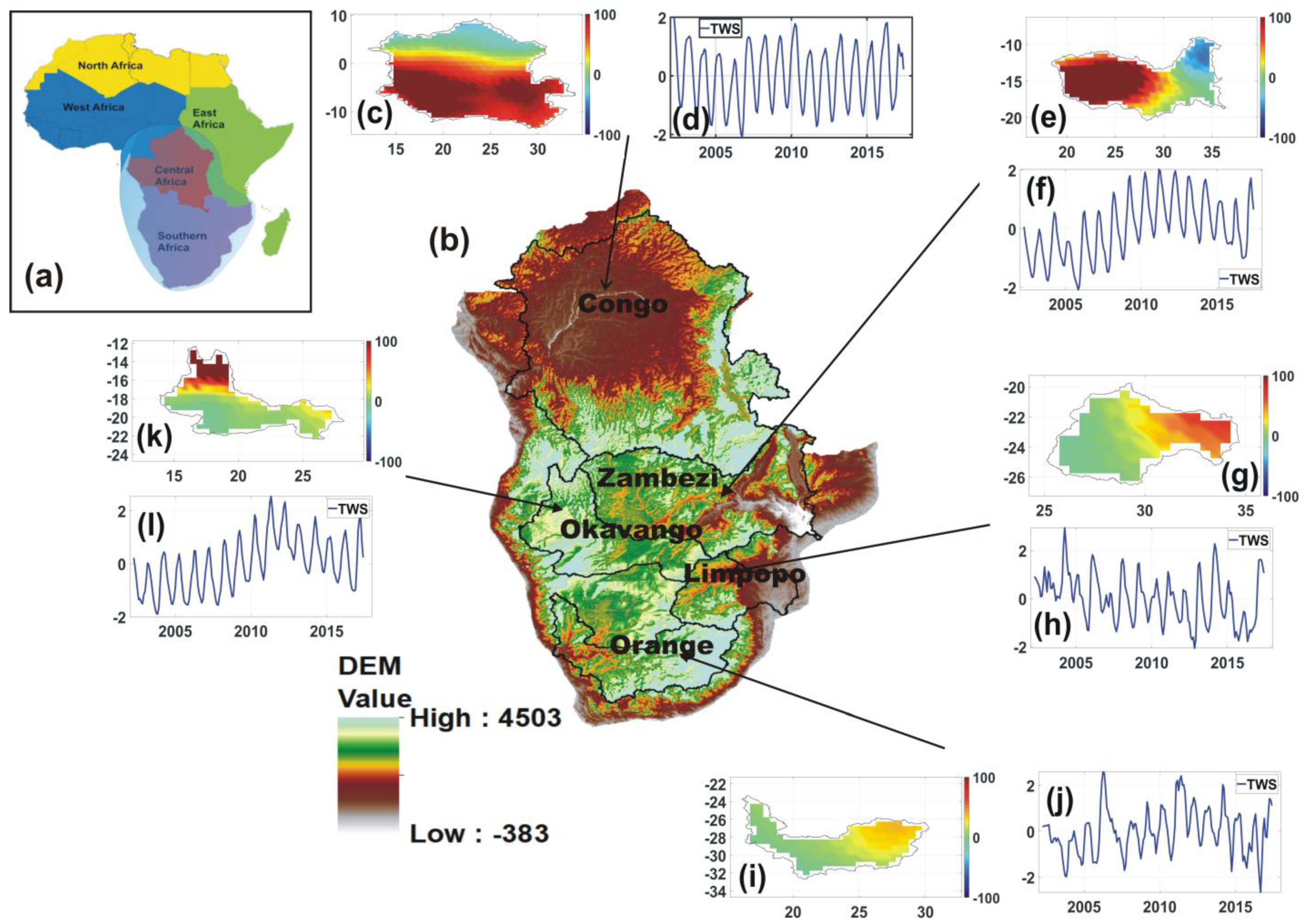
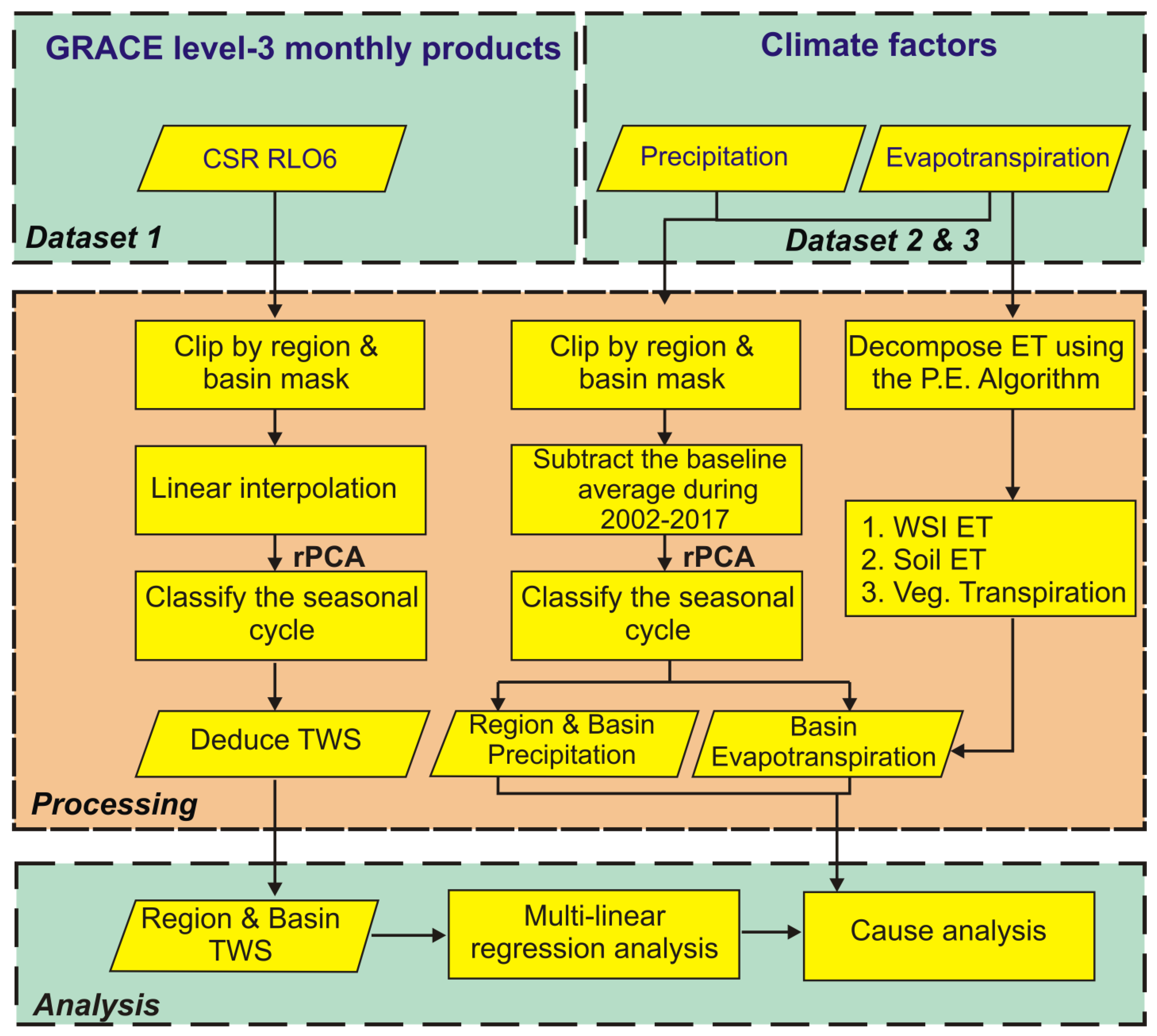
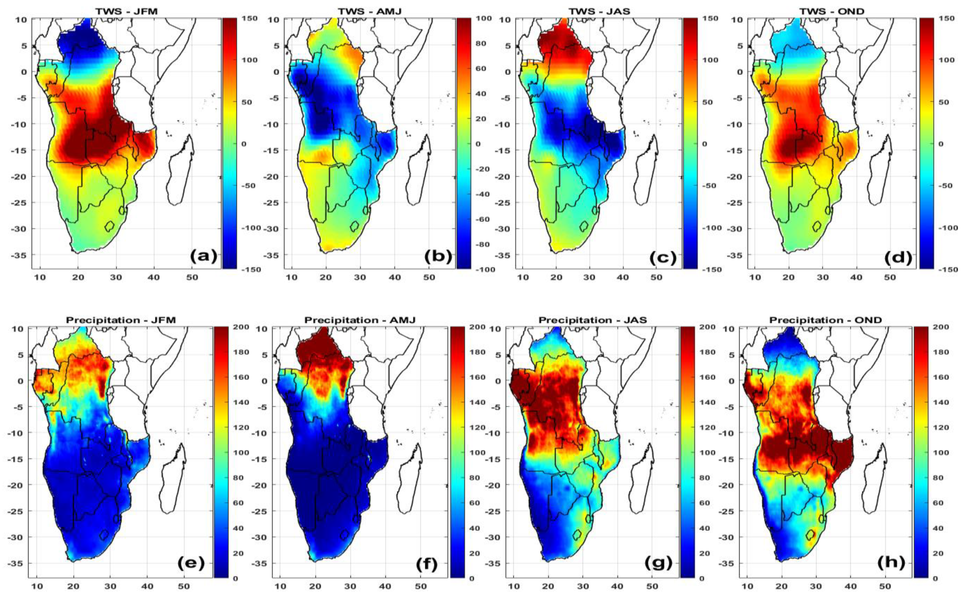
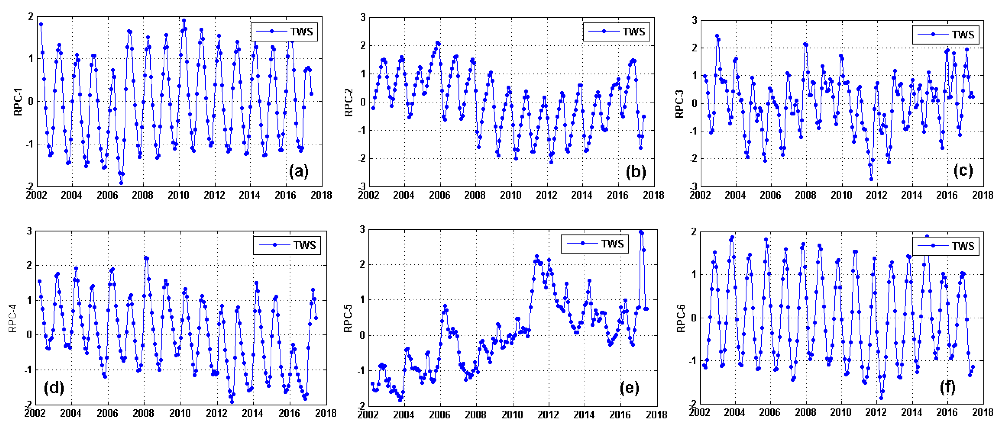
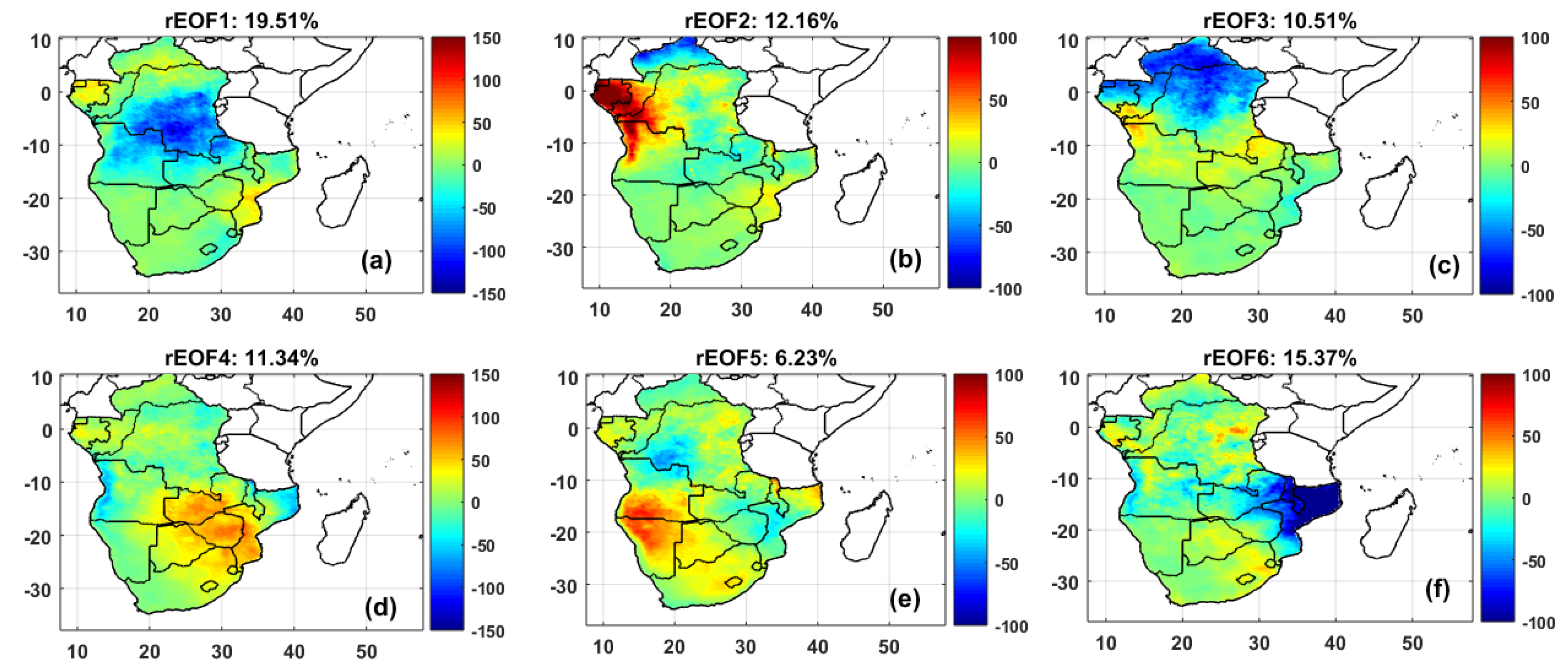
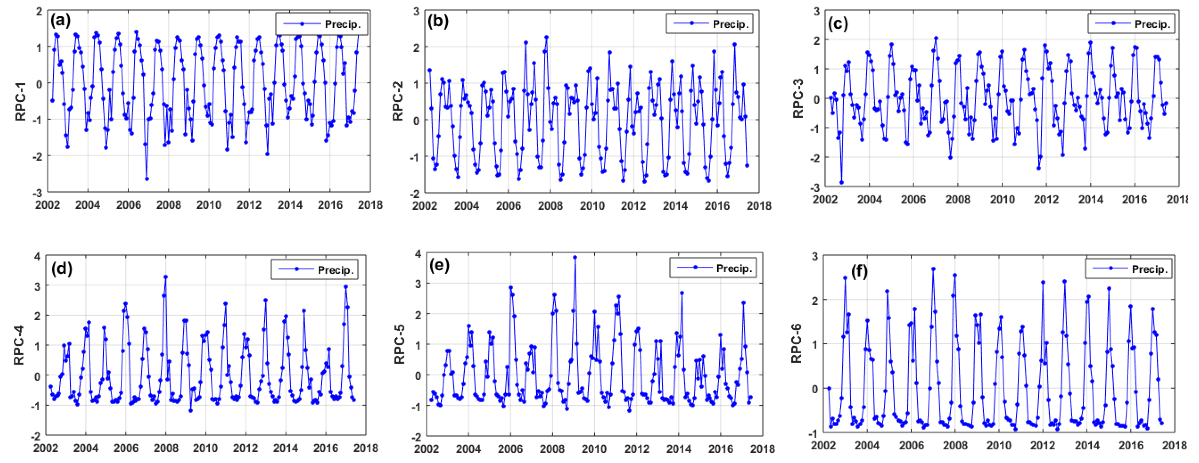
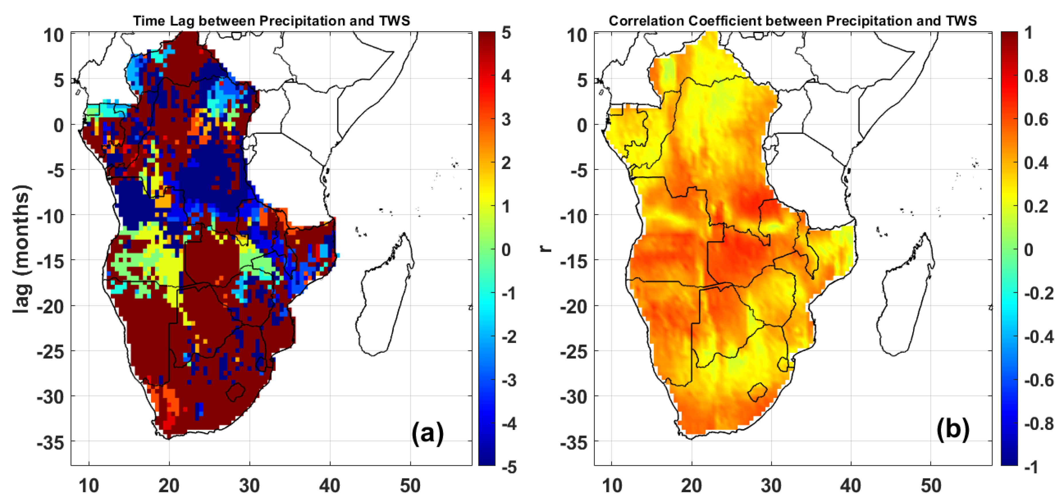
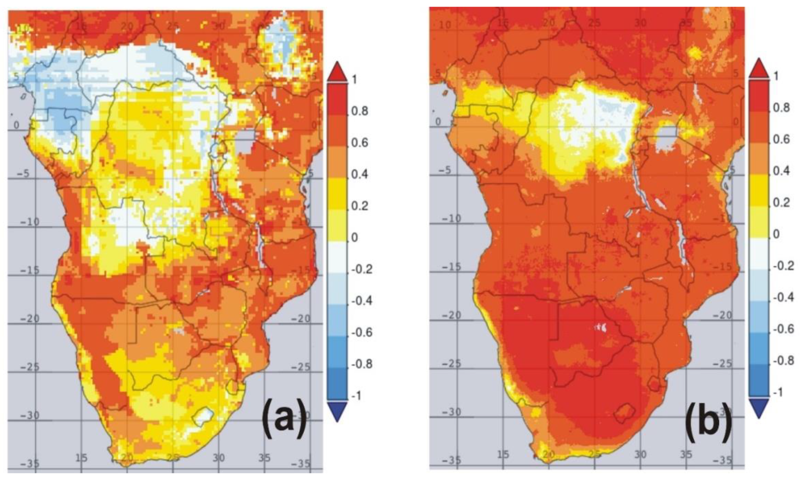
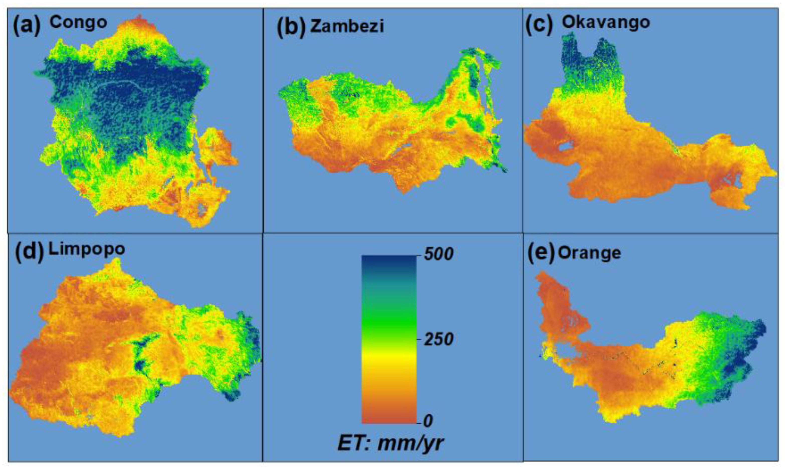
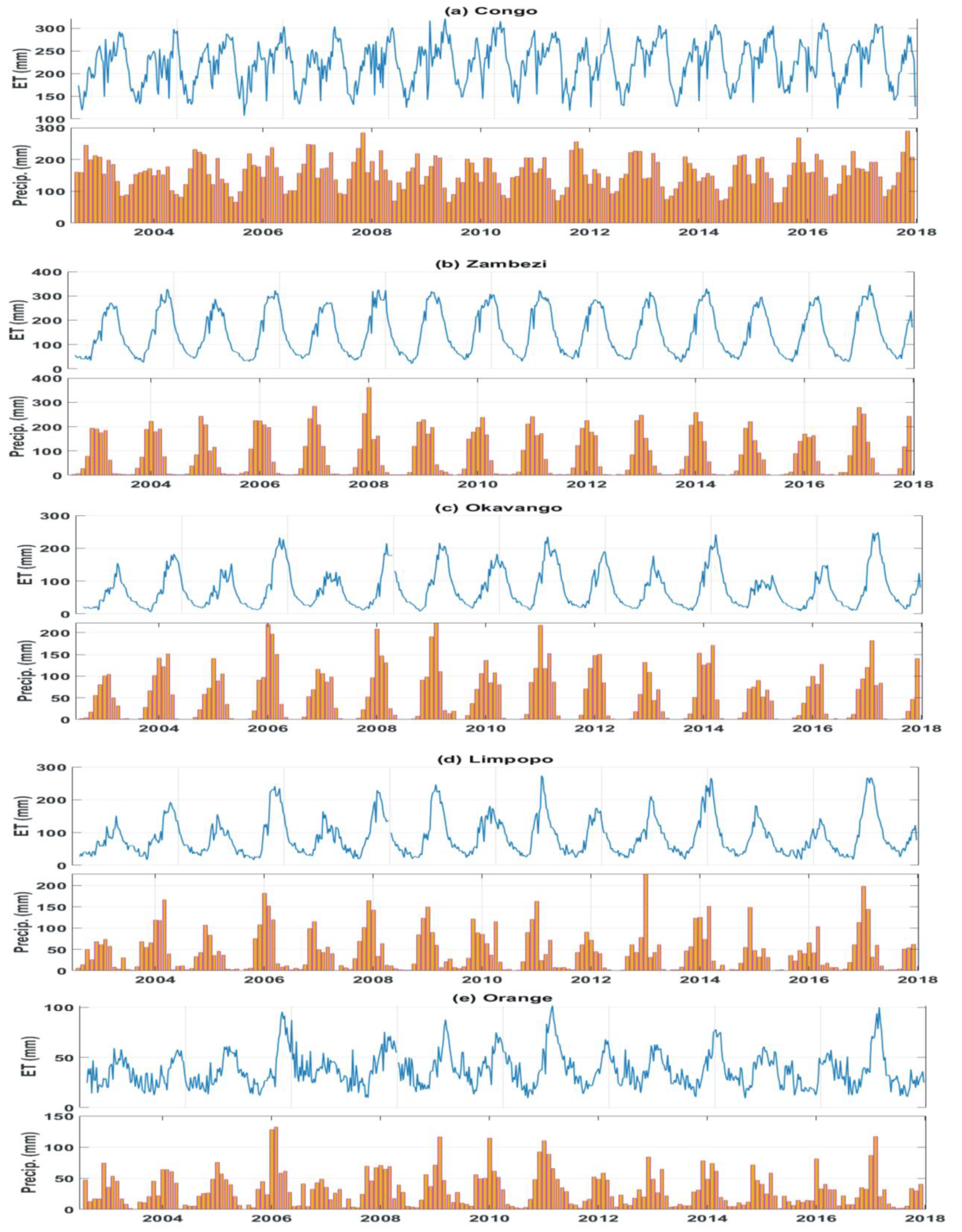
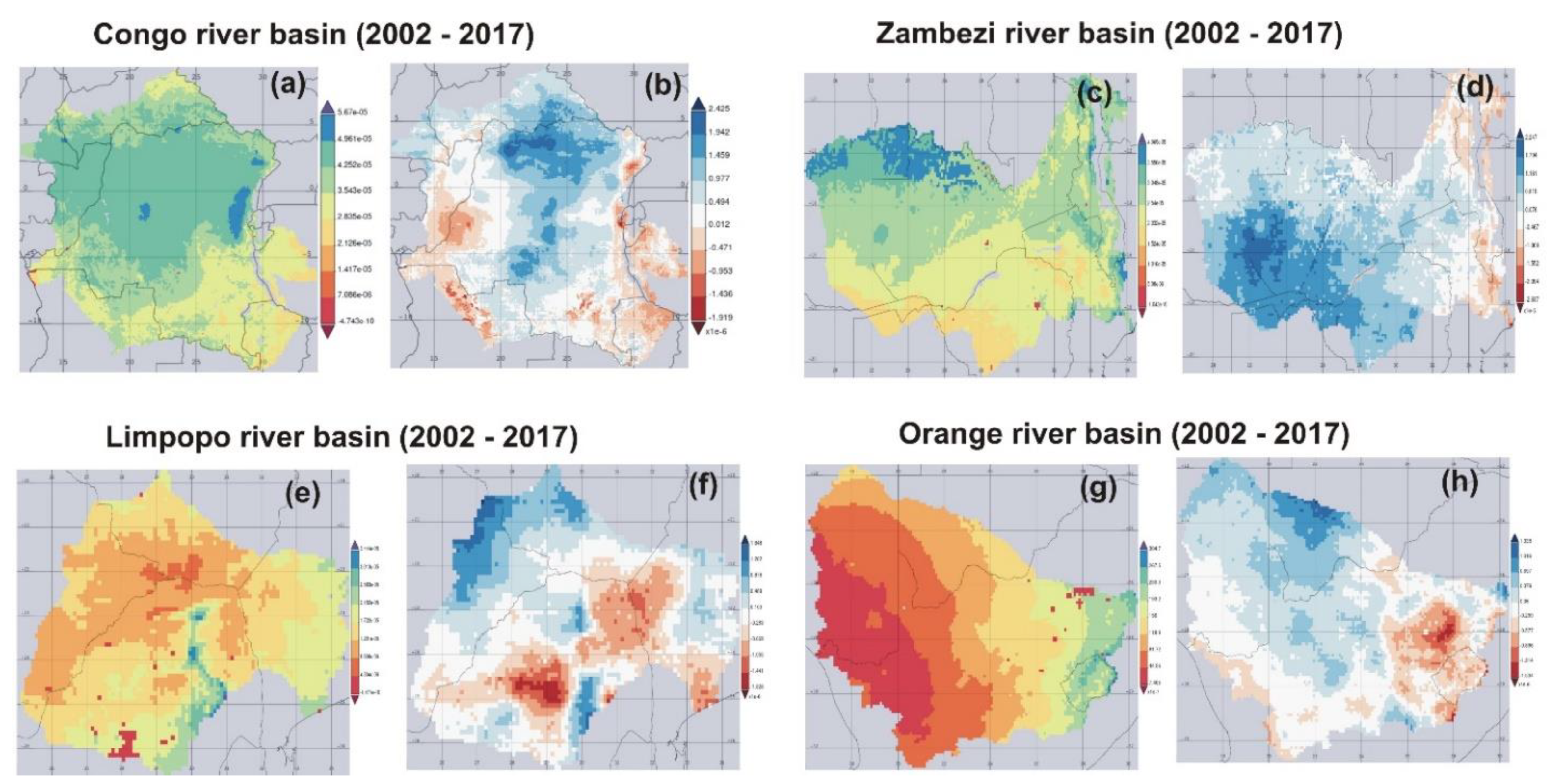
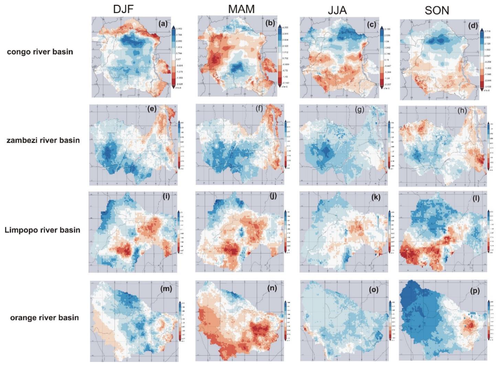
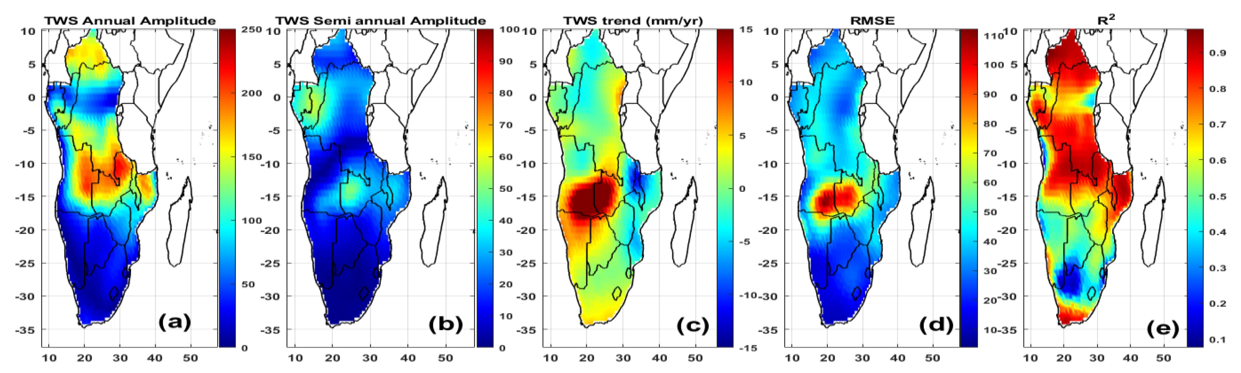
Table 1.
Using multi-linear regression to model the relationship between rotated parameters of TWS (Figure A3), precipitation, and evapotranspiration within the five major river basins in SCA from 2002 to 2017. The statistical report of each basin shows the relationship intercept (inter.) between the three products (unit:mm).
| Season 1 (mm) | Season 2 (mm) | |||||||||||
|---|---|---|---|---|---|---|---|---|---|---|---|---|
| MAM | SON | DJF | JJA | |||||||||
| Congo | Precip. | ET | TWS | Precip. | ET | TWS | Precip. | ET | TWS | Precip. | ET | TWS |
| 2002–2005 | 156.772 | 259.734 | 34.164 | 189.533 | 220.851 | −39.895 | 173.778 | 222.397 | 7.188 | 94.859 | 159.000 | −9.608 |
| 2006–2009 | 178.930 | 269.651 | 31.731 | 197.548 | 225.421 | −37.553 | 165.339 | 223.229 | 16.444 | 101.620 | 173.736 | −7.742 |
| 2010–2013 | 156.468 | 276.589 | 34.055 | 198.000 | 230.575 | −39.571 | 160.657 | 230.122 | 5.543 | 98.352 | 169.323 | −7.678 |
| 2014–2017 | 167.161 | 285.055 | 34.288 | 203.525 | 234.968 | −33.505 | 176.155 | 225.200 | 10.579 | 92.006 | 179.884 | −1.068 |
| MLRS (r2 = 0.86) | MLRS (r2 = 0.70) | MLRS (r2 = 0.43) | MLRS (r2 = 0.97) | |||||||||
| Inter. | Precip. | ET | Inter. | Precip. | ET | Inter. | Precip. | ET | Inter. | Precip. | ET | |
| Coefficients | 39.212 | −0.105 | 0.043 | −114.90 | 0.616 | −0.194 | 328.4 | −0.325 | −1.170 | −19.424 | −0.473 | 0.344 |
| SE | 12.916 | 0.044 | 0.044 | 60.027 | 0.844 | 0.793 | 382.6 | 0.647 | 1.351 | 0.505 | 0.004 | 0.002 |
| t-stat | 3.036 | −2.371 | 0.973 | −1.914 | 0.729 | −0.244 | 0.858 | −0.502 | −0.866 | −38.427 | −122.7 | 187.9 |
| p-value | 0.203 | 0.254 | 0.509 | 0.306 | 0.599 | 0.847 | 0.548 | 0.704 | 0.546 | 0.017 | 0.005 | 0.003 |
| Zambezi | Precip. | ET | TWS | Precip. | ET | TWS | Precip. | ET | TWS | Precip. | ET | TWS |
| 2002–2005 | 75.902 | 205.660 | −3.464 | 40.358 | 67.479 | −46.536 | 196.487 | 227.456 | −30.230 | 3.498 | 62.780 | −26.195 |
| 2006–2009 | 75.304 | 219.480 | 25.761 | 50.665 | 70.255 | −29.783 | 226.659 | 246.941 | −4.481 | 3.584 | 71.700 | −7.224 |
| 2010–2013 | 69.459 | 222.093 | 52.580 | 41.369 | 68.772 | −2.369 | 210.376 | 247.376 | 22.071 | 2.747 | 73.425 | 23.216 |
| 2014–2017 | 67.022 | 235.552 | 35.658 | 38.985 | 63.851 | −17.309 | 206.849 | 220.576 | −2.289 | 2.017 | 78.682 | 8.623 |
| MLRS (r2 = 0.58) | MLRS (r2 = 0.30) | MLRS (r2 = 0.32) | MLRS (r2 = 0.63) | |||||||||
| Inter. | Precip. | ET | Inter. | Precip. | ET | Inter. | Precip. | ET | Inter. | Precip. | ET | |
| Coefficients | 97.314 | −2.670 | 0.554 | −36.412 | −0.844 | 0.718 | −220.8 | 0.175 | 0.765 | −152.6 | −3.196 | 2.256 |
| SE | 1038.6 | 7.122 | 2.542 | 559.6 | 5.518 | 10.690 | 327.9 | 1.933 | 1.772 | 311.8 | 29.728 | 3.295 |
| t-stat | 0.094 | −0.375 | 0.218 | −0.065 | −0.153 | 0.067 | −0.674 | 0.091 | 0.432 | −0.490 | −0.107 | 0.684 |
| p-value | 0.941 | 0.772 | 0.863 | 0.959 | 0.903 | 0.957 | 0.623 | 0.942 | 0.740 | 0.710 | 0.931 | 0.617 |
| Okavango | Precip. | ET | TWS | Precip. | ET | TWS | Precip. | ET | TWS | Precip. | ET | TWS |
| 2002–2005 | 48.394 | 96.183 | 3.554 | 30.949 | 30.236 | −46.440 | 122.255 | 116.138 | −25.229 | 1.004 | 25.584 | −27.257 |
| 2006–2009 | 52.284 | 119.4 | 18.956 | 34.915 | 37.150 | −34.824 | 133.424 | 126.539 | −10.341 | 1.919 | 33.857 | −12.933 |
| 2010–2013 | 52.000 | 110.6 | 53.192 | 27.020 | 31.979 | 2.030 | 130.352 | 144.269 | 25.114 | 0.211 | 32.052 | 22.812 |
| 2014–2017 | 53.134 | 125.5 | 36.653 | 24.495 | 29.230 | −13.523 | 107.856 | 103.461 | 8.698 | 0.447 | 35.710 | 3.083 |
| MLRS (r2 = 0.90) | MLRS (r2 = 0.89) | MLRS (r2 = 0.77) | MLRS (r2 = 0.74) | |||||||||
| Inter. | Precip. | ET | Inter. | Precip. | ET | Inter. | Precip. | ET | Inter. | Precip. | ET | |
| Coefficients | −1031.4 | 28.665 | −3.676 | −18.414 | −7.580 | 6.770 | 78.722 | −2.662 | 2.035 | −69.80 | −18.45 | 2.602 |
| SE | 370.7 | 10.858 | 1.783 | 64.775 | 2.626 | 3.403 | 120.9 | 1.695 | 1.123 | 81.226 | 14.415 | 2.484 |
| t-stat | −2.782 | 2.639 | −2.061 | −0.284 | −2.886 | 1.989 | 0.650 | −1.569 | 1.812 | −0.859 | −1.280 | 1.047 |
| p-value | 0.219 | 0.230 | 0.287 | 0.823 | 0.212 | 0.29656 | 0.632 | 0.361 | 0.320 | 0.548 | 0.422 | 0.485 |
| Limpopo | Precip. | ET | TWS | Precip. | ET | TWS | Precip. | ET | TWS | Precip. | ET | TWS |
| 2002–2005 | 40.590 | 102.9 | 34.516 | 32.196 | 55.592 | −5.225 | 97.689 | 125.187 | 20.885 | 6.924 | 41.705 | 14.045 |
| 2006–2009 | 34.794 | 111.0 | 21.857 | 48.033 | 69.659 | −26.013 | 95.596 | 154.971 | 9.905 | 7.450 | 43.273 | −4.163 |
| 2010–2013 | 37.059 | 99.025 | 13.401 | 39.023 | 71.945 | −38.622 | 97.666 | 165.082 | 2.153 | 2.671 | 43.659 | −15.499 |
| 2014–2017 | 41.420 | 122.3 | 18.160 | 31.257 | 60.737 | −35.082 | 84.744 | 130.925 | −1.485 | 3.614 | 44.882 | −10.508 |
| MLRS (r2 = 0.19) | MLRS (r2 = 0.78) | MLRS (r2 = 0.92) | MLRS (r2 = 0.79) | |||||||||
| Inter. | Precip. | ET | Inter. | Precip. | ET | Inter. | Precip. | ET | Inter. | Precip. | ET | |
| Coefficients | 1.653 | 1.271 | −0.262 | 83.50 | 1.583 | −2.625 | −77.30 | 1.533 | −0.408 | 249.9 | 1.908 | −6.081 |
| SE | 115.2 | 2.803 | 0.841 | 61.48 | 1.398 | 1.416 | 43.377 | 0.504 | 0.163 | 272.4 | 3.314 | 6.010 |
| t-stat | 0.014 | 0.453 | −0.312 | 1.358 | 1.132 | −1.853 | −1.782 | 3.041 | −2.492 | 0.917 | 0.575 | −1.011 |
| p-value | 0.990 | 0.728 | 0.807 | 0.404 | 0.460 | 0.315 | 0.325 | 0.202 | 0.242 | 0.527 | 0.667 | 0.496 |
| Orange | Precip. | ET | TWS | Precip. | ET | TWS | Precip. | ET | TWS | Precip. | ET | TWS |
| 2002–2005 | 31.337 | 39.957 | −0.414 | 23.069 | 24.352 | −34.727 | 64.836 | 48.230 | −14.147 | 15.558 | 25.973 | −14.304 |
| 2006–2009 | 34.784 | 43.702 | 23.055 | 33.690 | 32.632 | −16.943 | 62.698 | 53.558 | 3.824 | 13.092 | 31.926 | 0.951 |
| 2010–2013 | 33.685 | 42.074 | 40.082 | 19.569 | 24.390 | −10.084 | 67.482 | 58.898 | 15.848 | 9.257 | 29.815 | 18.970 |
| 2014–2017 | 28.538 | 42.570 | 28.366 | 21.774 | 24.523 | −28.804 | 49.993 | 44.461 | −2.719 | 8.647 | 28.090 | −3.549 |
| MLRS (r2 = 0.43) | MLRS (r2 = 0.97) | MLRS (r2 = 0.99) | MLRS (r2 = 0.64) | |||||||||
| Inter. | Precip. | ET | Inter. | Precip. | ET | Inter. | Precip. | ET | Inter. | Precip. | ET | |
| Coefficients | −274.0 | −0.192 | 7.201 | −151.5 | −7.037 | 11.389 | −64.532 | −1.554 | 3.128 | −48.342 | −2.230 | 2.584 |
| SE | 347.6 | 4.914 | 8.673 | 28.186 | 1.600 | 2.446 | 10.217 | 0.255 | 0.314 | 112.3 | 2.661 | 3.440 |
| t-stat | −0.788 | −0.039 | 0.830 | −5.377 | −4.398 | 4.655 | −6.315 | −6.090 | 9.953 | −0.430 | −0.838 | 0.751 |
| p-value | 0.575 | 0.975 | 0.5588 | 0.117 | 0.142 | 0.134 | 0.0999 | 0.103 | 0.063 | 0.741 | 0.555 | 0.589 |
Table 2.
Average annual Evapotranspiration of five major river basins in the SCA region during 2002–2017 (unit:mm) data for 2002* started in July.
Table 2.
Average annual Evapotranspiration of five major river basins in the SCA region during 2002–2017 (unit:mm) data for 2002* started in July.
| Basin | 2002* | 2003 | 2004 | 2005 | 2006 | 2007 | 2008 | 2009 | 2010 | 2011 | 2012 | 2013 | 2014 | 2015 | 2016 | 2017 |
|---|---|---|---|---|---|---|---|---|---|---|---|---|---|---|---|---|
| Congo | 193.1 | 214.9 | 211.8 | 218.4 | 221.6 | 218.2 | 216.5 | 230.0 | 236.0 | 224.0 | 215.9 | 227.6 | 230.5 | 228.6 | 230.8 | 234.0 |
| Zambezi | 73.4 | 137.8 | 160.4 | 126.5 | 158.6 | 142.1 | 150.7 | 161.8 | 160.8 | 158.5 | 144.8 | 145.3 | 155.1 | 141.2 | 144.8 | 171.7 |
| Okavango | 32.8 | 55.4 | 78.1 | 60.6 | 97.5 | 56.0 | 81.0 | 89.6 | 84.3 | 95.8 | 73.7 | 62.1 | 93.5 | 50.1 | 62.5 | 101.9 |
| Limpopo | 46.5 | 70.5 | 90.8 | 66.2 | 103.5 | 83.5 | 83.4 | 103.5 | 93.8 | 94.9 | 77.8 | 88.3 | 106.3 | 68.6 | 71.2 | 116.6 |
| Orange | 29.2 | 31.6 | 32.6 | 34.6 | 49.2 | 33.6 | 39.3 | 42.0 | 38.7 | 45.2 | 38.8 | 34.1 | 40.9 | 31.8 | 34.5 | 38.3 |
Table 3.
Average annual precipitation of five major river basins in the SCA region during 2002–2017 (unit:mm) data for 2002* started in July.
Table 3.
Average annual precipitation of five major river basins in the SCA region during 2002–2017 (unit:mm) data for 2002* started in July.
| Basin | 2002* | 2003 | 2004 | 2005 | 2006 | 2007 | 2008 | 2009 | 2010 | 2011 | 2012 | 2013 | 2014 | 2015 | 2016 | 2017 |
|---|---|---|---|---|---|---|---|---|---|---|---|---|---|---|---|---|
| Congo | 195.3 | 151.5 | 156.8 | 144.7 | 170.6 | 169.7 | 152.6 | 152.2 | 155.2 | 160.2 | 155.5 | 147.6 | 142.0 | 155.9 | 158.4 | 170.6 |
| Zambezi | 62.3 | 77.3 | 88.0 | 69.2 | 90.2 | 88.9 | 90.3 | 86.4 | 84.4 | 84.2 | 79.1 | 72.6 | 82.4 | 64.5 | 72.2 | 95.4 |
| Okavango | 31.8 | 40.7 | 52.8 | 48.7 | 70.9 | 41.1 | 60.0 | 66.7 | 52.6 | 65.3 | 50.3 | 38.5 | 53.5 | 31.9 | 42.0 | 56.3 |
| Limpopo | 32.7 | 36.4 | 54.8 | 33.7 | 60.7 | 47.7 | 41.4 | 51.5 | 46.6 | 43.3 | 31.9 | 50.5 | 51.3 | 26.2 | 38.0 | 51.8 |
| Orange | 33.5 | 22.6 | 30.9 | 29.9 | 49.0 | 28.7 | 34.0 | 39.6 | 36.4 | 39.7 | 31.0 | 27.3 | 31.2 | 20.2 | 29.0 | 31.9 |
Table 4.
TWS gain/loss per cycle for major river basins in the SCA region based on the rPCA technique (unit:mm) 2002 and 2017 consists of some missing months.
Table 4.
TWS gain/loss per cycle for major river basins in the SCA region based on the rPCA technique (unit:mm) 2002 and 2017 consists of some missing months.
| Basin | 2002 | 2003 | 2004 | 2005 | 2006 | 2007 | 2008 | 2009 | 2010 | 2011 | 2012 | 2013 | 2014 | 2015 | 2016 | 2017 |
|---|---|---|---|---|---|---|---|---|---|---|---|---|---|---|---|---|
| Congo | - | 0.232 | −0.266 | −0.375 | −0.687 | 0.196 | 0.165 | 0.180 | 0.292 | −0.271 | −0.197 | 0.032 | 0.008 | −0.035 | 0.324 | - |
| Zambezi | - | −0.930 | −0.496 | −1.228 | −0.662 | −0.538 | −0.036 | 0.482 | 0.717 | 0.915 | 0.824 | 0.679 | 0.636 | 0.187 | −0.251 | - |
| Okavango | - | −1.017 | −0.581 | −0.797 | −0.635 | −0.570 | −0.314 | 0.074 | 0.435 | 1.331 | 1.081 | 0.528 | 0.568 | 0.108 | −0.012 | - |
| Limpopo | - | 0.420 | 1.063 | −0.162 | 0.599 | −0.447 | 0.023 | 0.143 | −0.239 | −0.082 | −0.892 | −0.263 | 0.536 | −0.705 | −1.119 | - |
| Orange | - | −0.950 | −0.726 | −0.542 | 1.125 | −0.662 | −0.162 | 0.015 | 0.059 | 1.424 | 0.448 | 0.261 | 0.299 | −0.344 | −0.596 | - |
Publisher’s Note: MDPI stays neutral with regard to jurisdictional claims in published maps and institutional affiliations. |
© 2021 by the authors. Licensee MDPI, Basel, Switzerland. This article is an open access article distributed under the terms and conditions of the Creative Commons Attribution (CC BY) license (https://creativecommons.org/licenses/by/4.0/).
Share and Cite
MDPI and ACS Style
Kalu, I.; Ndehedehe, C.E.; Okwuashi, O.; Eyoh, A.E. Assessing Freshwater Changes over Southern and Central Africa (2002–2017). Remote Sens. 2021, 13, 2543. https://0-doi-org.brum.beds.ac.uk/10.3390/rs13132543
AMA Style
Kalu I, Ndehedehe CE, Okwuashi O, Eyoh AE. Assessing Freshwater Changes over Southern and Central Africa (2002–2017). Remote Sensing. 2021; 13(13):2543. https://0-doi-org.brum.beds.ac.uk/10.3390/rs13132543
Chicago/Turabian StyleKalu, Ikechukwu, Christopher E. Ndehedehe, Onuwa Okwuashi, and Aniekan E. Eyoh. 2021. "Assessing Freshwater Changes over Southern and Central Africa (2002–2017)" Remote Sensing 13, no. 13: 2543. https://0-doi-org.brum.beds.ac.uk/10.3390/rs13132543
Note that from the first issue of 2016, this journal uses article numbers instead of page numbers. See further details here.