
Measurement of Snow Water Equivalent Using Drone-Mounted Ultra-Wide-Band Radar


1
Department of Physics and Technology, UiT The Arctic University of Norway, 9019 Tromsø, Norway
2
NORCE Norwegian Research Centre, 9019 Tromsø, Norway
*
Author to whom correspondence should be addressed.
†
These authors contributed equally to this work.
Remote Sens. 2021, 13(13), 2610; https://0-doi-org.brum.beds.ac.uk/10.3390/rs13132610
Submission received: 4 May 2021
/
Revised: 21 June 2021
/
Accepted: 25 June 2021
/
Published: 2 July 2021
(This article belongs to the Special Issue Remote Sensing in Glaciology and Cryosphere Research)
Abstract
:The use of unmanned aerial vehicle (UAV)-mounted radar for obtaining snowpack parameters has seen considerable advances over recent years. However, a robust method of snow density estimation still needs further development. The objective of this work is to develop a method to reliably and remotely estimate snow water equivalent (SWE) using UAV-mounted radar and to perform initial field experiments. In this paper, we present an improved scheme for measuring SWE using ultra-wide-band (UWB) (0.7 to 4.5 GHz) pseudo-noise radar on a moving UAV, which is based on airborne snow depth and density measurements from the same platform. The scheme involves autofocusing procedures with the frequency–wavenumber (F–K) migration algorithm combined with the Dix equation for layered media in addition to altitude correction of the flying platform. Initial results from field experiments show high repeatability (R > 0.92) for depth measurements up to m, and good agreement with Monte Carlo simulations for the statistical spread of snow density estimates with standard deviation of g/cm3. This paper also outlines needed system improvements to increase the accuracy of a snow density estimator based on an F–K migration technique.
1. Introduction
There is a vast variety of applications for drone-mounted radar including archaeological investigations; detection of buried mines [1,2]; soil moisture mapping [3], snow, ice, and glacier measurements [4,5]; and mapping of civil infrastructure [6,7]. With regards to snow, one application is snow water equivalent (SWE) measurements, which is of great interest for the hydropower industry and other disciplines in need of meteorological data.
Today, ground-based SWE surveys (manual or with ground penetrating radar (GPR)) are usually conducted by means of snowmobile, where avalanche safety and accessibility might reduce the survey area [8,9,10].
The ground below the snowpack in mountainous and marshland areas often contains sparse scattering objects, potentially producing diffraction hyperbolas in a radar B-scan. These objects are usually rocks with a relative permittivity (∼4–7) that is different from snow. Migration methods applied on radar imagery at the correct propagation velocity of the intermediate medium cause the hyperbolas to collapse at their focal point. Previous studies using commercial GPR, mounted on a snowmobile, show that SWE can be estimated using frequency–wavenumber (F–K) migration and manual velocity picking [8]. A similar method also demonstrates autofocusing using the varimax norm to automatically pick the velocity [11], and similar results can be produced from offset antenna arrays [12]. Furthermore, Kirchhoff’s time migration with a two-layered variable-depth velocity model was used to focus radar image GPR data from a helicopter platform [5]. Recent work shows the use of a commercially available, lightweight, and small form-factor 24-GHz radar for drone-mounted measurements of lake ice and SWE measurements of dry snow from a stationary platform with a known snow depth [13].
Other work show SWE estimation using manually measured snow depth, snow age, and snow class defined by the location [14]. Manual depth measurements at calibration locations can also be used to estimate SWE with radars [15]. Alternatively, by combining two way travel time (TWT) with meteorological models obtained from empirical studies, SWE can be estimated from quasi-analytical expressions [16]. This latter model generalizes the snowpack layer model for which the density depends on depth. The assumption might be acceptable for applications that only need coarse density estimations. However, the scheme needs modifications for each new climatic zone (maritime or continental climate) to be valid [16]. Additionally, common mid-point (CMP) gathers can also be used to extract the dielectric permittivity of snow [17]. Several studies take the concept a step forward and outline methods for automatic detection and segmentation of diffraction hyperbolas. This research includes novel image threshold methods and clustering [18], parabolic fitting [19], apex detection by fitting an analytical hyperbola function to the profile edges detected with a Canny filter [20], template matching algorithms [21], and a neural network approach [22]. SWE can also be estimated on a large scale using neural networks to perform a nonlinear mapping between datasets of manual measurements to predict SWE [23], and by combining snow model simulation, manual measurements, and auxiliary products derived from remote sensing in a k-nearest neighbors (k-NN) algorithm [24].
This paper presents a technological approach to SWE measurements by using ultra-wide-band (UWB) radar mounted on an autonomous flying unmanned aerial vehicle (UAV). The method involves estimating snow depth and density by using well-established F–K migration theory and the Dix equation for layered media in addition to altitude correction of the flying platform. The goal is to estimate propagation velocity in the snow using air-launched UWB signals with significant separation (∼5–10 m) between the radar platform and medium of interest (snowpack) compared to GPR at ground level. This is accomplished by analyzing diffraction hyperbolas in B-scan radar images, described in the following sections.
2. Materials and Methods
2.1. Theory
This section covers the main method used for SWE estimation and the theory behind the different steps. We assume that the radar image is already preprocessed with both matched filtering and frequency-domain noise filtering. These basic preprocessing steps for the UWB radar data are described in more detail in [25,26].
2.1.1. Altitude Correction
As the UAV performs an airborne survey of an area, the aircraft’s altitude will inevitably vary somewhat, at least on a medium to large spatial scale. The altitude variations depend on what sensors the UAV computer has available to feed into the autopilot. In our setup, we have a laser rangefinder [27] that measures relative altitude on a centimeter scale and provides real-time feedback to the autopilot. Nevertheless, minor deviations in the altitude regulation will distort the radar image. Hence, the radar data algorithms need some correction to “level out” these variations.
The method used in this work is to circularly shift the radar data in the fast-time direction according to the relative variations in altitude. The rectification is performed by combining the laser range data and the first surface pulse reflection in the radar return. The combination of altitude information in these two signals reduces spurious deviations significantly and minimizes the influence of signal drop-out in the laser rangefinder.
Prior to migration, the sectioned data segment is expanded in fast-time according to the distance measured from the UAV to the snow surface. This method is explained in more detail in [26].
2.1.2. Methods to Estimate Propagation Velocity from Diffraction Hyperbolas
There are several different methods to estimate the propagation velocity of a radar signal return from an object [28]. Nonetheless, this paper will focus on estimating the propagation velocity by analyzing diffraction hyperbolas in B-scan radar images. In a B-scan GPR image, diffraction hyperbolas are manifested as “south-opening” branches [18]. If diffraction hyperbolas are present in the radar image, there are generally two different procedures to extract the bulk propagation velocity information:
As previously stated, hyperbolas contain information about the mean propagation velocity in the medium. Hence, if we know the parameters that mathematically describe the hyperbola, we can estimate the propagation velocity [30] by the simple relation between the hyperbola asymptotic constants a and b. Thus, the velocity can be calculated from [31]:
where a and b need to be in their correct units, namely, seconds and meters, respectively.
Autofocusing is performed by testing different propagation velocities in a migration process where we assess how well the image is focused in order to determine the mean propagation velocity (see example in Section 2.3).
2.1.3. Autofocusing Metrics
Autofocusing techniques are widely used in, for example, synthetic aperture radar (SAR) applications for phase error correction [32,33,34], and for GPR, usually to estimate the dielectric constant [29,35,36,37]. Autofocusing generally works by testing different propagation velocities with a migration algorithm outputting a migrated image and choosing the best fitting velocity based on some performance metric.
Since the apex of the hyperbolas should have a maximum at the correct propagation velocity, we can look at the average image intensity to evaluate the focusing [29]. For a migrated radar image at test velocity , this parameter can be stated as
where . The size of the image is represented by m and n as the slow-time and fast-time samples, respectively.
However, this metric is known to have poor performance for increasing signal to noise ratio (SNR) [38]. Thus, higher-order techniques that involve the variance of the migrated image [38] can be expressed by
where , and and are the mean and variance of the migrated data, respectively.
As in [38], a k value of 10 was found to be optimal. AH will have a maximum at the best fitting propagation velocity representing the mean propagation velocity along the antenna-to-target trajectory.
2.1.4. Dix’s Equation
We emphasize that the best fit velocity represents the average velocity from the antennas to the hyperbola. Hence, to remove the influence of the air section to calculate the average propagation velocity in the snow itself, Dix’s equation for layered media can be used [39]:
where is the total TWT in the medium, is the TWT of the air layer, and is the approximate propagation velocity in the atmosphere (i.e., approximately m/ns).
2.1.5. Estimation of Snow Parameters
Snow depth is usually measured by evaluating the TWT from the snow surface to the ground and calculating the distance traveled based on an estimate of the propagation velocity.
For lossless, homogeneous, isotropic materials, the relative propagation velocity in the snow is related to the relative dielectric constant by [30]:
where c is the propagation velocity in free space. The depth is then simply written as
where is the TWT from the snow surface to the ground. Equation (5) states that the relative dielectric constant is nonlinearly related to the propagation velocity. From this relation, there are several different models for estimating the density of snow.
The relation between snow permittivity and density has been modeled both theoretically [40] and empirically [41]. Considering dry snow, a linear relationship is an acceptable approximation for snow densities below g cm−3, where the relation between the real part of the relative dielectric constant and relative snow density can be modeled as [41]
where is relative density compared with the density of water (1 g/cm3). SWE is the depth of water resulting from the mass of melted snow and typically expressed in millimeters of equivalent water [42]. The SWE is the product of the snow depth and the vertically integrated snow density, and can be expressed as
Furthermore, SWE is often used to estimate the total precipitation in a given location and the resulting water volume available for the melt season.
2.2. Radar System
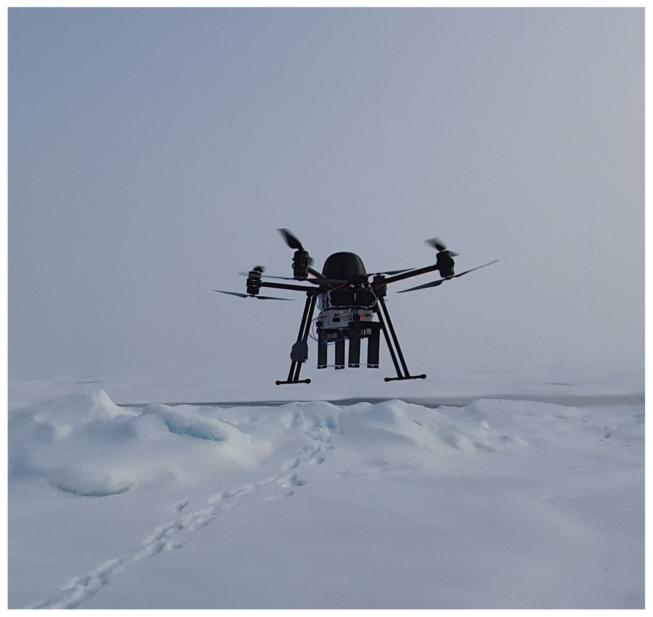
The ultra-wideband snow sounder (UWiBaSS) is a custom-developed radar system for drone-mounted snow measurements. Papers [25,26,43] detail recent advances of the radar system. New developments include retrofitting the radio frequency (RF) operation band as well as digital modules with 3D printed casings coated in conductive paint to reduce weight while still offering electromagnetic interference (EMI) protection. Additionally, 500-MHz high-pass filters are added to the receiving (RX) channels to reduce low-frequency antenna cross-talk. Table 1 summarizes main features of the UWB-system while Figure 1 shows the UAV “Cryocopter FOX” during flight.
2.3. Processing Flow
The basic preprocessing steps for the sampled radar data involve match filtering to correlate the received signal with the transmitted signal, high-pass filtering to remove low-frequency cross-talk between receiving (RX) and transmitting (TX) antennas, reference subtraction, and altitude correction involving rectification of the snow surface return. A detailed description can be found in [26].
The laser altimeter measures the distance to the snow surface. By locating the first interface reflection, the radar is capable of similar distance measurements. We have found that the best practice is to use a combination of both sensors in case of laser signal drop out, which possibly occurs when the laser altimeter beam strikes large snow crystals at an angle.
A distance-vector representing traveled distance over the snow surface is calculated using the position data collected from the UAV autopilot. Using the Haversine formula, we calculate the distance between each coordinate point to generate the distance vector. Due to the non-equidistant sampling of this vector, the radar data goes through a nonlinear interpolation in the slow-time direction. This procedure interpolates the radar data into a domain with equidistant position samples in space, allowing us to fix the sampling interval instead of calculating a mean value for each segment.
Hyperbolas in the radar image are segmented manually using a simple “draw rectangle” function, creating a slow-time section of the image to focus within. Furthermore, fast-time data outside the rectangular window is set to zero. Although not implemented here, this step can be automated [18].
The method averages altimeter data within each short section (5 to 20 m). Further, we add zeros to the top of the radar image corresponding to the actual scanning platform altitude above the snow surface, effectively recreating the “real” radar scenario.
Figure 2 shows an example image of the processed radar data before the autofocusing procedure.
Autofocusing
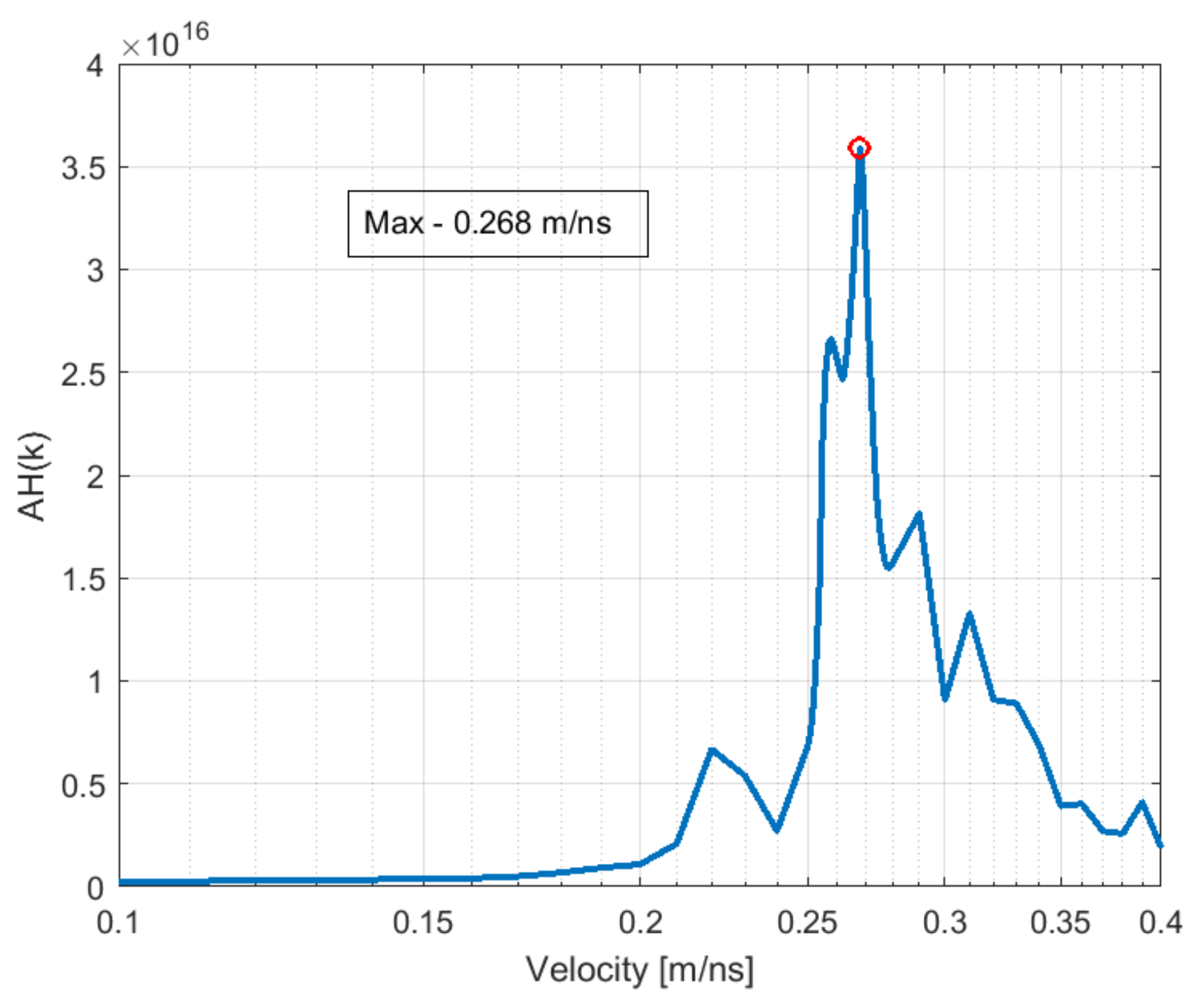
The autofocusing procedure involves performing F–K migration for a set of test velocities, where autofocusing metrics are calculated for each test velocity. In order to reduce the numerical calculation time, the search for the optimal velocity can be done in several different ways, such as first performing a low-resolution scan over a broad spread of velocities before performing a high-resolution scan over a much more narrow interval. For the present tests, we used a brute force linear vector in two steps. First a coarse search was performed with step value of m/ns to scan through an interval from 0.1 to 0.4 m/ns. Thereafter, a fine search was used with step value of m/ns to scan through an interval from 0.25 to 0.3 m/ns.
F–K migration was performed with the CREWES MatLab toolbox written by G. F. Margrave for the CREWES project (University of Calgary) [44,45]. The F–K domain interpolation routine was modified with a convolution, omitting a for-loop in order to reduce the computational time. This modification improved the speed of the function by approximately 200%.
After migration over all test velocities, we selected the autofocusing metric’s (see Equation (3)) maximal value, corresponding to a “best fit” propagation velocity. This velocity represents the average velocity from the radar antennas to the ground; therefore, we need to remove the influence of the air section with Dix’s equation. This estimation is performed for each manually selected section. The section length is typically in the range of 5 to 20 m containing one or more hyperbolas. Figure 3 shows an example of the autofocusing result for a segment gathered as in Figure 2. Figure 4 shows the combined autofocusing result of the coarse and fine search.
2.4. Monte Carlo Simulation of FK-Migration Method
Monte Carlo simulation is a numerical experimentation technique to obtain the statistics of the output variables of a computational model [46]. The proposed method discussed above involves several steps using error-prone parameters. The parameters include altitude and position data from the UAV dataflash-log applied to calculate the distance and the altitude vectors. These vectors position the data in 2D-space and are essential inputs to the migration algorithm.
In this section, we evaluate the uncertainty of the method by creating synthetic data sets of a single hyperbola in a homogeneous medium. The synthetic data is F–K migrated and combined with Equation (3), resulting in an estimate for . Further, using Equations (4) (giving ), (5), and (7), we calculate the bulk dielectric constant and density of the snowpack.
The altitude and distance vectors are given random errors set to adequate values for our imaging system to make the simulations relevant for real data results. Specifically, the synthetic data parameters are given values similar to the field experiment data in Section 3.1, with a fixed snow-depth of 2 m and an initial altitude (above the snow surface) of 7 m over a horizontal distance of 15 m. The mean propagation velocity is set to m/ns, resulting in a snow velocity of m/ns after Dix equation analysis.
2.4.1. Laser Altimeter Error Sources
The SF-11 rangefinder data-sheet [27] reports an accuracy of cm. Additionally, the laser is not always pointing in nadir due to the attitude of the UAV, which is corrected through the attitude data (roll, pitch, yaw). However, given that the UAV often flies over uneven terrain, additional errors are expected.
The rangefinder error is assumed to be normally distributed in the Monte Carlo analysis, with a standard deviation of 15 cm deemed reasonable. The altitude error contributes twice to the erroneous estimations since it is part of two parameters in the method: firstly, prior to the focusing when the length of the fast-time vector is adjusted according to the altitude above the surface; secondly, in the time parameter when Dix’s equation is applied.
2.4.2. Distance Error Sources
The distance vector is calculated using the Haversine formula [47] on the filtered position data produced by the UAV autopilot. The position estimate is the output of the autopilot extended Kalman filter (EKF). The EKF estimates vehicle position, velocity, and angular orientation based on rate gyroscopes, accelerometer, compass (magnetometer), global positioning system (GPS), airspeed, and barometric pressure measurements. Concerning the method proposed in this paper, the error can be defined as the deviation from linear movement (constant horizontal velocity), as the absolute position is not relevant for the focusing procedure. In real data, the deviation from a perfectly linear equidistant distance vector (i.e., constant horizontal velocity) was approximately m, when looking at real data sets from autonomous flights. Therefore, we choose a standard deviation slightly larger than this ( m) as a conservative assumption for the error analysis.
The distance error is applied to the data by interpolating the synthetic data set along the distance axis according to the linear movement deviation, producing non-equidistant sampling. As expected, the interpolation procedure causes some skewness in the hyperbola that influences the statistical results (see the following subsection).
2.4.3. Monte Carlo Simulation Results
An essential prerequisite of the autofocusing method under study is that it is unbiased to produce a close-to-correct estimate of the sought parameter (snow density or SWE) mean value.
The Anderson–Darling, Jarque–Bera, and Chi-square tests [48,49,50] all indicate that the results from the Monte Carlo simulations are normally distributed both in the bivariate case and with the errors combined, as in Figure 5. As seen in Figure 5, the velocity estimates are unbiased, with a standard deviation of /.
Introducing Dix’s equation in Figure 5b causes further uncertainties in the estimate since we use the erroneous altitude once more. However, the method is still unbiased, with an increased standard deviation of /. Since the estimation of in Figure 5c involves squaring of the velocity estimates, the distribution (if assumed normal) is transformed to a Chi-square distribution of order 1. However, if the standard deviation is significantly smaller than the mean, the Chi-square distribution can be approximated as normally distributed. Finally, the approximate linear relationship in Equation (7) is used to obtain the distribution in Figure 5d.
We now compare the Monte-Carlo-derived results with the theoretically approximated first two moments derived in Appendix A. Using = 0.234 m/nsecs and = 0.0147 m/nsecs in Equations (A9) and (A10), we obtain = 1.639 (1.6% deviation) and = 0.205 (5% deviation). Furthermore, using Equations (A12) and (A13), we obtain = 0.319 g/cm (2.6% deviation) and = 0.103 g/cm (4.6% deviation); all results compared to values in Figure 5c.
The Monte Carlo simulations emphasize the need for accurate positioning for the presented method as the relative spread of the density parameter is relatively large compared to the mean value ( = 0.33). Nonetheless, using the average of several estimates to reduce the estimator spread could be a useful approach as the snow density spatial variability is expected to be much smaller than local variations in snow depth [51].
3. Results
3.1. Field Experiments
Due to Covid-19, two major field campaigns were canceled in the winter of 2020. However, a 1-day campaign 10 km from UiT The Arctic University of Norway was carried out. The main goal of the campaign was to test the latest iteration of the radar system and preliminarily investigate methods to measure snow density.
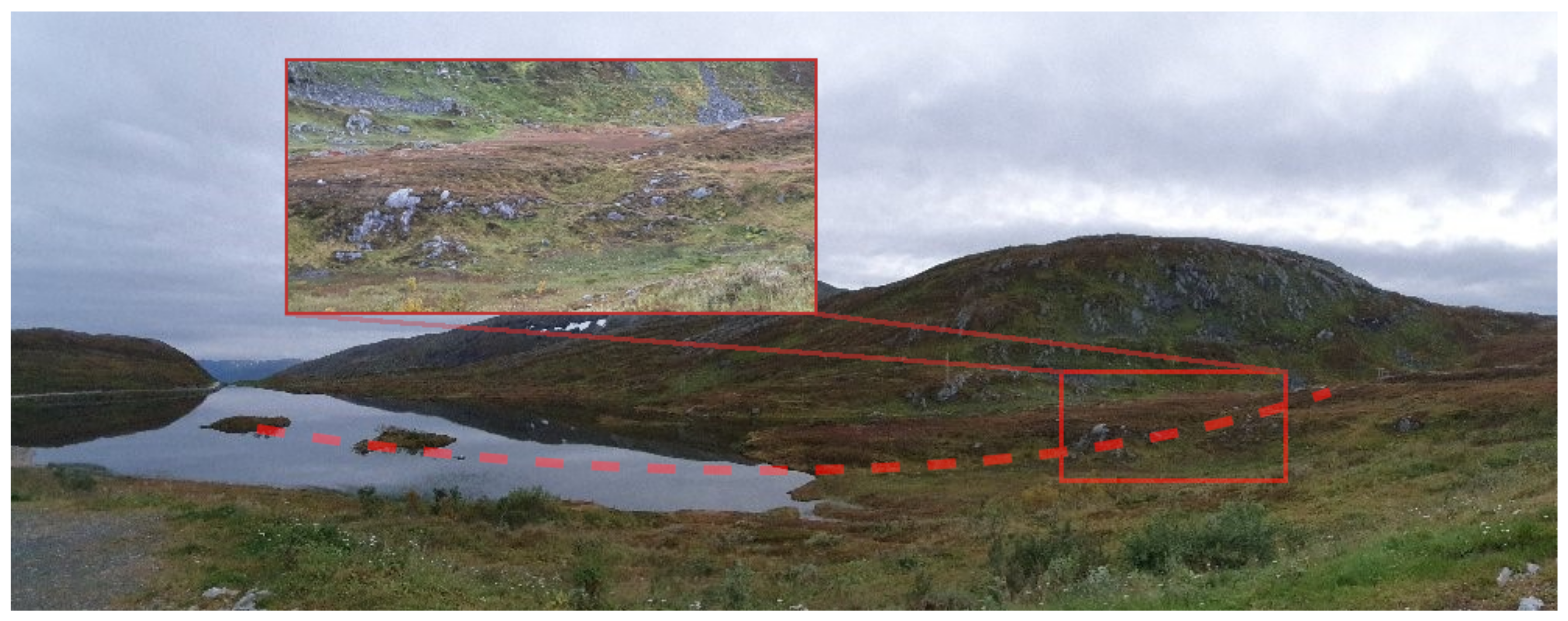
A transect of approximately 250 m was flown autonomously for four passes to test the reproducibility of the method. A section of the transect showed several overlapping hyperbolas at the ground level (shown in Figure 2). These hyperbolas were assumed to be caused by reflections from rocks, as is well known from traditional GPR [30], but this is not necessarily the case given that the uwibass would be able to detect hyperbolas from targets buried beneath several meters of snow during flight. As shown in Figure 6 and Figure 7, the snow depth in this transect varied from 1 m to almost 6 m.
After the spring snowmelt, radar data images containing hyperbolas were confirmed to be from a rocky area, as shown in Figure 8.
Four passes over this rocky area of the transect were segmented into 40 smaller segments of varying size (5 to 20 m) used to estimate the density.
For this data set, the returning signal from the snowpack was taken at the second period of the transmitted signal owing to the radar system having a 5.9-m unambiguous range, and the data collection was taken from approximately 7-m relative altitude, excluding snow depth. For more information on performing measurements outside the unambiguous range from UAV radar, see [26].
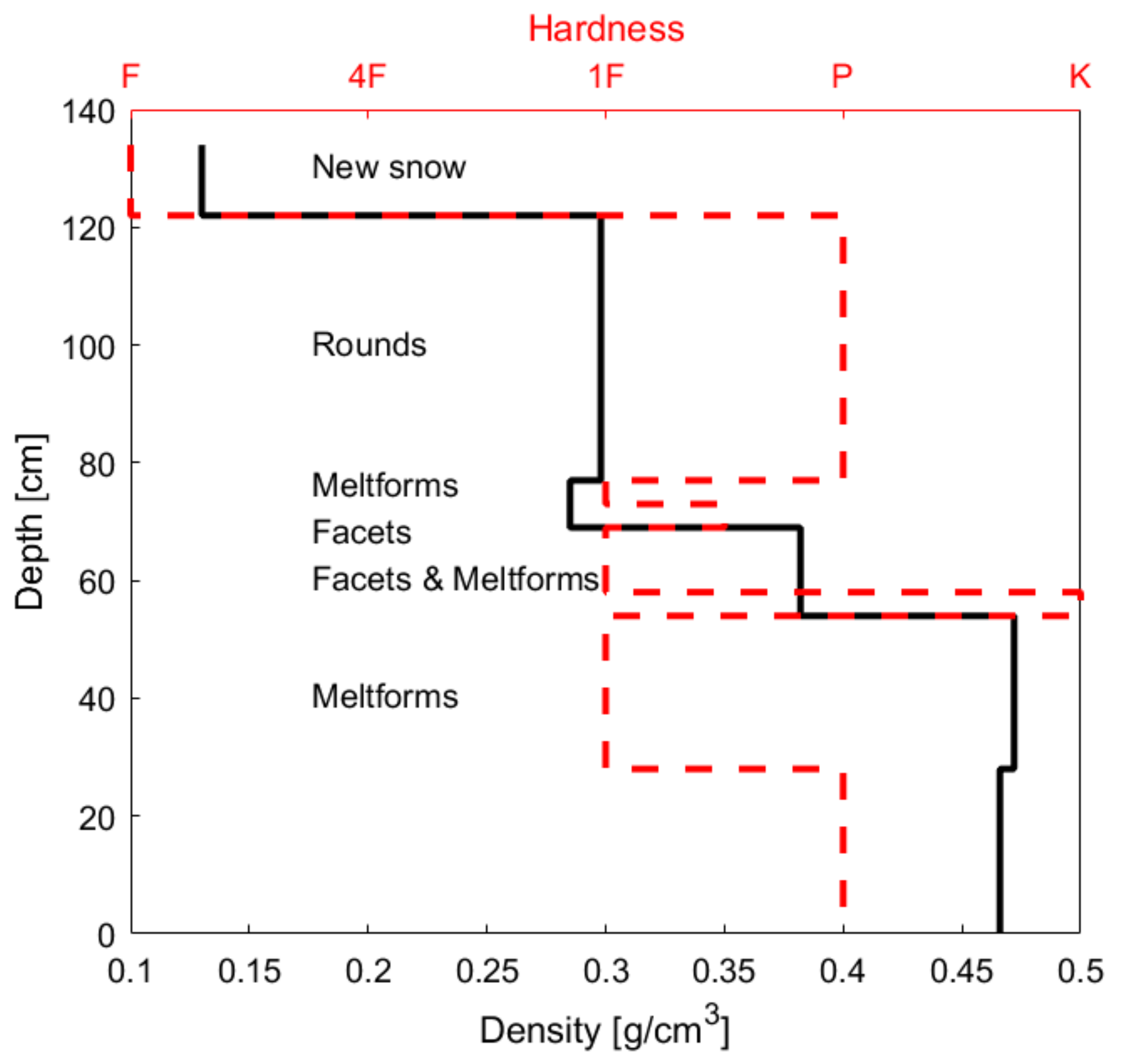
The in situ density for each noticeable layer was collected in a snow pit close to the transect. We found the weighted density average (weighted mean based on the thickness of each layer) to be g cm−3. Figure 9 shows the snow pit density profile along with hardness and grain type. Grain size was 1 to 2 mm.
Figure 10 shows the distribution of density estimations from the autofocusing procedure. Figure 6 shows measured snow depth along the 250-m transect for four passes. Identification of the snow–ground interface is described in [26], where we obtained the TWT used in Equation (6). Snow depth is then calculated using the TWT and the estimated propagation velocity of the snow.
4. Discussion
The accuracy of the method seems to depend heavily on the accuracy of the recorded UAV position, since the spatial sampling rate and correct position and altitude above snow are important for the F–K migration algorithm. Hence, real-time kinematic (RTK) GPS should be used for better distance calculations and data interpolation [52]. Taking the average of the altitude for each section will, in most cases, not introduce significant errors, as the typical variation in altitude across the sections is on the order of a few cm. However, for robustness, modifying the code to create a variable altitude above the snow should be implemented in future work [5].
Ideally, several snow pits should have been dug along the transect. However, the time constraints of the project limited the in situ collection to one full snow pit.
Comparing Figure 5d with Figure 10, we see that the statistical spread (standard deviation) is of the same order, which leads us to believe that the error assessments made to the scanning system prior to the Monte Carlo simulation were reasonable and that other contributing error sources are of minor importance in the campaign.
The standard deviation ( g/cm3 from Figure 10) of the estimations are comparable to what is observed in previous papers [8], reporting a standard deviation of g/cm3 from a snowmobile platform with a fixed antenna-to-snow air gap of approximately 50 cm.
The degree to which the snow depth measurements can be trusted is of vital importance when determining the SWE. A comparison of depth measurements for several passes along the same transect gives a good indication of the repeatability of depth measurements. This can be seen for four passes in Figure 6 and for two passes overlaid on the radar B-scan in Figure 7. Correlating the four transects results in the correlation matrix R:
Overall, the correlation is very high, with the lowest value of 0.92 between passes 2 and 4. The slight skewness between the depth measurements in Figure 6 appears to come from drift in the UAV positioning. Hence, the repeatability of snow depth measurements will likely also benefit from more accurate positioning such as RTK GPS. The snow depth is measured beyond 5 m, which is deeper than the 3-m depth probes we had available. However, in situ snow depth validation of the same radar system has been presented in [26].
Notice in Figure 2 that the reconstructed radar pulse delay becomes almost 90 ns, resulting in a total distance from the antennas to the ground of approximately 10 to 14 m. With an unambiguous range of m, this is accomplished by exploiting the lack of significant reflections in the air-section except for the cross-talk [26] and, thus, using the previously transmitted pulse for detection.
The area coverage of this UAV-mounted radar system is small compared to satellite remote sensing products [24]. However, the high spatial resolution generated by the UAV-mounted radar has the opportunity to detect local variability, resulting in more accurate SWE measurements.
5. Conclusions
In this paper, we present a noninvasive method to estimate snow density from a UAV that could be further used to estimate SWE. Density estimations from a limited field trial show good agreement with in situ snow density, and snow depth measurements show high repeatability. However, the sample size for both in situ and radar data is somewhat limited.
Future work will include field campaigns with RTK-ready UAV for improved position and altitude information, as well as high-resolution in situ density measurements using the SnowMicroPen (SMP) or similar devices. Additionally, automatic image segmentation should be implemented to reduce the amount of manual labor to analyze the data sets. Multithreaded programming should be implemented on the interpolation part of the F–K migration routine to improve speed, as this section of the code occupies approximately 95% of the run time.
Author Contributions
Conceptualization, R.O.R.J. and S.K.J.; methodology, R.O.R.J. and S.K.J.; software, R.O.R.J.; validation, R.O.R.J.; formal analysis, R.O.R.J.; investigation, R.O.R.J.; writing—original draft preparation, R.O.R.J.; writing—review and editing, R.O.R.J. and S.K.J. All authors have read and agreed to the published version of the manuscript.
Funding
This work was supported by the Centre for Integrated Remote Sensing and Forecasting for Arctic Operations (CIRFA) partners (Grant No. 237906); and NORCE Norwegian Research Centre (Grant No. 261786); Research Council of Norway.
Acknowledgments
The authors would like to thank M. Eckerstorfer and A. Kjellstrup for collecting in situ data and operating the UAV during the field experiments. The authors acknowledge the useful comments by four anonymous reviewers that helped improve the readability of this study.
Conflicts of Interest
The authors declare no conflict of interest.
Appendix A. Mapping of Squared Inverse Gaussian Variable
Consider a Gaussian variable X with standard deviation and mean value . Then, defining
is centrally chi-square-distributed with one degree of freedom.
Knowing that = 1 and = 2 in a central chi-squared distribution, the first and second moments of X can be stated:
where the approximations are valid if —that is, a narrow probability distribution of X.
Mapping a Gaussian variable X with the relation , we obtain the probability density function (pdf) [53]:
Notice that, for situations where , the last term in Equation (A4) can be neglected unless w and are close to zero.
Then, Equation (A4) can be stated:
Furthermore, Taylor series expanding the argument in the exponential function to second order around the central value of the distribution, and similarly approximating the denominator , we obtain
We recognize Equation (A6) as a Gaussian distribution with standard deviation and mean value , in accordance with the results obtained in Equations (A2) and (), if .
The permittivity of snow is related to propagation velocity v through , where c is the speed of light in air. In order to relate this mapping to Equation (A6), define the reciprocal variable . Now, it can readily be shown that
Once again, Taylor expanding to zeroth order and Taylor expanding the argument of the exponential function to second order, both around , Equation (A7) reduces to
From Equation (A8), we see that u is also normally distributed with a mean value and standard deviation .
Furthermore, the constant R can be identified as and , leading to the final result that is close to normally distributed with first and second moments:
provided that .
According to [41], there exists a linear relation between the dielectric constant and density in dry snow:
This leads to the first and second moments of :
Hence, we obtain a constant change in mean value and spread in the probability distribution of 1/2 as expected from a linear transformation.
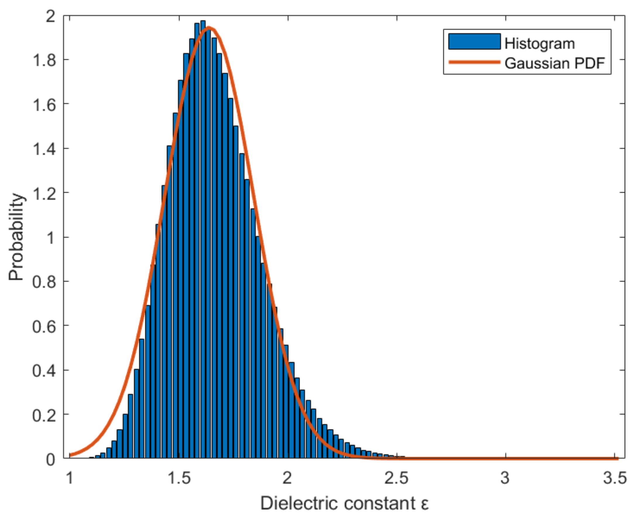
As an example, assume a statistical draw of v from a Gaussian distribution. Figure A1 shows the histogram from 100,000 statistical realizations mapped by using with first and second moments of snow velocity of 0.244 m/nsecs and 0.0127 m/nsecs, respectively.
Figure A1.
Histogram of dielectric constant from 100,000 realizations. Solid line: Gaussian approximation from Equation (A8). Mean value and standard deviation are = 1.51 and = 0.16, respectively.
Figure A1.
Histogram of dielectric constant from 100,000 realizations. Solid line: Gaussian approximation from Equation (A8). Mean value and standard deviation are = 1.51 and = 0.16, respectively.

Observe that the fit between the histogram and the theoretical approximate Gaussian distribution is not perfect, as the assumption that is not entirely fulfilled.
References
- Cerquera, M.R.P.; Colorado Montaño, J.D.; Mondragón, I.; Montaño, J.D.C.; Mondragón, I. UAV for Landmine Detection Using SDR-Based GPR Technology. In Robots Operating in Hazardous Environments; Intech Open: Bogotá, Colombia, 2016; p. 13. [Google Scholar]
- Šipoš, D.; Peter, P.; Gleich, D. On drone ground penetrating radar for landmine detection. In Proceedings of the 2017 First International Conference on Landmine: Detection, Clearance and Legislations (LDCL), Beirut, Lebanon, 26–28 April 2017; pp. 7–10. [Google Scholar] [CrossRef]
- Wu, K.; Rodriguez, G.A.; Zajc, M.; Jacquemin, E.; Clément, M.; De Coster, A.; Lambot, S. A new drone-borne GPR for soil moisture mapping. Remote Sens. Environ. 2019, 235, 111456. [Google Scholar] [CrossRef]
- Tan, A.E.C.; McCulloch, J.; Rack, W.; Platt, I.; Woodhead, I. Radar Measurements of Snow Depth Over Sea Ice on an Unmanned Aerial Vehicle. IEEE Trans. Geosci. Remote Sens. 2020, 59, 1868–1875. [Google Scholar] [CrossRef]
- Rutishauser, A.; Maurer, H.; Bauder, A. Helicopter-borne ground-penetrating radar investigations on temperate alpine glaciers: A comparison of different systems and their abilities for bedrock mapping. Geophysics 2016, 81, WA119–WA129. [Google Scholar] [CrossRef]
- Greenwood, W.W.; Lynch, J.P.; Zekkos, D. Applications of UAVs in Civil Infrastructure. J. Infrastruct. Syst. 2019, 25, 04019002. [Google Scholar] [CrossRef]
- Li, C.J.; Ling, H. High-resolution, downward-looking radar imaging using a small consumer drone. In Proceedings of the 2016 IEEE International Symposium on Antennas and Propagation (APSURSI), Fajardo, PR, USA, 26 June–1 July 2016; Volume 2, pp. 2037–2038. [Google Scholar] [CrossRef]
- Holbrook, W.S.; Miller, S.N.; Provart, M.A. Estimating snow water equivalent over long mountain transects using snowmobile-mounted ground-penetrating radar. Geophysics 2016, 81, WA183–WA193. [Google Scholar] [CrossRef]
- Knut Sand, O.B.; Sand, K.; Bruland, O. Application of Georadar for snow cover surveying. Nord. Hydrol. 1998, 29, 361–370. [Google Scholar] [CrossRef]
- Derksen, C.; Toose, P.; Rees, A.; Wang, L.; English, M.; Walker, A.; Sturm, M. Development of a tundra-specific snow water equivalent retrieval algorithm for satellite passive microwave data. Remote Sens. Environ. 2010, 114, 1699–1709. [Google Scholar] [CrossRef]
- Clair, J.S.; Steven Holbrook, W. Measuring snow water equivalent from common-offset GPR records through migration velocity analysis. Cryosphere 2017, 11, 2997–3009. [Google Scholar] [CrossRef] [Green Version]
- Gustafsson, D.; Sundström, N.; Lundberg, A. Estimation of Snow Water Equivalent of Dry Snowpacks Using a Multi-Offset Ground Penetrating Radar System. In Proceedings of the 69th Eastern Snow Conference, Claryville, NY, USA, 5–7 June 2012; pp. 197–206. [Google Scholar]
- Pomerleau, P.; Royer, A.; Langlois, A.; Cliche, P.; Courtemanche, B.; Madore, J.B.; Picard, G.; Lefebvre, E. Low cost and compact FMCW 24 GHz radar applications for snowpack and ice thickness measurements. Sensors 2020, 20, 3909. [Google Scholar] [CrossRef]
- Bruland, O.; Færevåg, Å.; Steinsland, I.; Liston, G.E.; Sand, K. Weather SDM: Estimating Snow density with high precision using Snow depth and local climate. Hydrol. Res. 2015, 46, 494–506. [Google Scholar] [CrossRef]
- Webb, R.W. Using ground penetrating radar to assess the variability of snow water equivalent and melt in a mixed canopy forest, Northern Colorado. Front. Earth Sci. 2017, 11, 482–495. [Google Scholar] [CrossRef]
- Lundberg, A.; Richardson-Näslund, C.; Andersson, C. Snow density variations: Consequences for ground-penetrating radar. Hydrol. Process. 2006, 20, 1483–1495. [Google Scholar] [CrossRef]
- Liu, H.; Takahashi, K.; Sato, M. Measurement of dielectric permittivity and thickness of snow and ice on a brackish lagoon using GPR. IEEE J. Sel. Top. Appl. Earth Obs. Remote Sens. 2014, 7, 820–827. [Google Scholar] [CrossRef]
- Dou, Q.; Wei, L.; Magee, D.R.; Cohn, A.G. Real-Time Hyperbola Recognition and Fitting in GPR Data. IEEE Trans. Geosci. Remote Sens. 2017, 55, 51–62. [Google Scholar] [CrossRef] [Green Version]
- Zhou, X.; Chen, H.; Li, J. An Automatic GPR B-Scan Image Interpreting Model. IEEE Trans. Geosci. Remote Sens. 2018, 56, 3398–3412. [Google Scholar] [CrossRef]
- Mertens, L.; Persico, R.; Matera, L.; Lambot, S. Automated Detection of Reflection Hyperbolas in Complex GPR Images with No A Priori Knowledge on the Medium. IEEE Trans. Geosci. Remote Sens. 2016, 54, 580–596. [Google Scholar] [CrossRef]
- Sagnard, F.; Tarel, J.P. Template-matching based detection of hyperbolas in ground-penetrating radargrams for buried utilities. J. Geophys. Eng. 2016, 13, 491–504. [Google Scholar] [CrossRef]
- Birkenfeld, S. Automatic detection of reflexion hyperbolas in GPR data with neural networks. In Proceedings of the 2010 World Automation Congress, WAC 2010, Kobe, Japan, 19–23 September 2010. [Google Scholar]
- Ghanjkhanlo, H.; Vafakhah, M.; Zeinivand, H.; Fathzadeh, A. Prediction of snow water equivalent using artificial neural network and adaptive neuro-fuzzy inference system with two sampling schemes in semi-arid region of Iran. J. Mt. Sci. 2020, 17, 1712–1723. [Google Scholar] [CrossRef]
- De Gregorio, L.; Günther, D.; Callegari, M.; Strasser, U.; Zebisch, M.; Bruzzone, L.; Notarnicola, C. Improving SWE estimation by fusion of snow models with topographic and remotely sensed data. Remote Sens. 2019, 11, 2033. [Google Scholar] [CrossRef] [Green Version]
- Jenssen, R.O.R.; Eckerstorfer, M.; Jacobsen, S. Drone-Mounted Ultrawideband Radar for Retrieval of Snowpack Properties. IEEE Trans. Instrum. Meas. 2020, 69, 221–230. [Google Scholar] [CrossRef] [Green Version]
- Jenssen, R.O.R.; Jacobsen, S. Drone-mounted UWB snow radar: Technical improvements and field results. J. Electromagn. Waves Appl. 2020, 34, 1930–1954. [Google Scholar] [CrossRef]
- Lightware. SF11 Laser altimeter Datasheet. 2018. Available online: https://www.documents.lightware.co.za/SF11%20-%20Laser%20Altimeter%20Manual%20-%20Rev%209.pdf (accessed on 1 June 2020).
- Serkan, S.; Borecky, V. Estimation Methods for Obtaining GPR Signal Velocity. In Proceedings of the Third Interlational Conference on ACSEE, Zurich, Switzerland, 10–11 October 2015; pp. 43–47. [Google Scholar] [CrossRef]
- Wei, X.; Zhang, Y. Autofocusing techniques for GPR data from RC bridge decks. IEEE J. Sel. Top. Appl. Earth Obs. Remote Sens. 2014, 7, 4860–4868. [Google Scholar] [CrossRef]
- Daniels, D. Ground Penetrating Radar, 2nd ed.; Institution of Engineering and Technology: London, UK, 2013; pp. 225–237. [Google Scholar]
- Alani, A.M.; Tosti, F. GPR applications in structural detailing of a major tunnel using different frequency antenna systems. Constr. Build. Mater. 2018, 158, 1111–1122. [Google Scholar] [CrossRef]
- Zhao, Y.; Gao, S.; Zhang, Z.; He, J.; Yu, W. An extended target autofocus algorithm for high resolution SAR imaging. In Proceedings of the International Conference on Radar Systems (Radar 2017), Belfast, UK, 23–26 October 2017; pp. 1–5. [Google Scholar] [CrossRef]
- Wahl, D.E.; Eichel, P.H.; Ghiglia, D.C.; Jakowatz, C.V. Phase Gradient Autofocus—A Robust Tool for High Resolution SAR Phase Correction. IEEE Trans. Aerosp. Electron. Syst. 1994, 30, 827–835. [Google Scholar] [CrossRef] [Green Version]
- Morrison, R.L.; Do, M.N.; Munson, D.C. SAR image autofocus by sharpness optimization: A theoretical study. IEEE Trans. Image Process. 2007, 16, 2309–2321. [Google Scholar] [CrossRef]
- Wei, X.; Zhang, Y. Interference Removal for Autofocusing of GPR Data from RC Bridge Decks. IEEE J. Sel. Top. Appl. Earth Obs. Remote Sens. 2015, 8, 1145–1151. [Google Scholar] [CrossRef]
- Qu, L.; Ge, Y.; Yang, T. Sparsity-based SFCW-GPR autofocusing imaging method under EM wave velocity uncertainty. Electron. Lett. 2017, 53, 568–570. [Google Scholar] [CrossRef]
- Jung, H.; Kim, K. Iteration Strategy for Autofocusing Metric Evaluation in GPR Imaging. In Proceedings of the ISAP 2018—2018 International Symposium on Antennas and Propagation, Busan, Korea, 23–26 October 2018; pp. 24–25. [Google Scholar]
- Wei, X. Gpr Data Processing for Reinforced Concrete Bridge Decks. Ph.D. Thesis, Georgia Institute of Technology, Atlanta, GA, USA, 2014. [Google Scholar]
- Dix, C.H. Seismic velocities from surface measurements. Geophysics 1955, 20, 68–86. [Google Scholar] [CrossRef]
- Tsang, L.; Kong, J.A. Scattering of electromagnetic waves from random media with multiple scattering included. J. Math. Phys. 1982, 23, 1213–1222. [Google Scholar] [CrossRef]
- Tiuri, M.; Sihvola, A.; Nyfors, E.; Hallikaiken, M. The complex dielectric constant of snow at microwave frequencies. IEEE J. Ocean. Eng. 1984, 9, 377–382. [Google Scholar] [CrossRef]
- Fierz, C.; Armstrong, R.; Durand, Y.; Etchevers, P.; Greene, E.; McClung, D.M.; Nishimura, K.; Satayawali, P.; Sokratov, S. The International Classification for Seasonal Snow on the Ground; IACS, UNESCO: Paris, France, 2009. [Google Scholar]
- Jenssen, R.O.R.; Eckerstorfer, M.; Jacobsen, S.K.; Storvold, R. Drone-Mounted UWB Radar System for Measuring Snowpack Properties: Technical Implementation, Specifications and Initial Results. Int. Snow Sci. Workshop 2018, 22, 673–676. [Google Scholar]
- Margrave, G.F. CREWES MatLab Toolbox. 2020. Available online: https://www.crewes.org/ResearchLinks/FreeSoftware/ (accessed on 12 June 2020).
- Margrave, G.F. Numerical Methods of Exploration Seismology; Department of Geology and Geophysics, The University of Calgary: Calgary, CA, USA, 2003. [Google Scholar]
- Harrison, R.L. Introduction to Monte Carlo simulation. In AIP Conference Proceedings; American Institute of Physics: College Park, MD, USA, 2009; Volume 1204, pp. 17–21. [Google Scholar] [CrossRef] [Green Version]
- Hegde, V.; Aswathi, T.S.; Sidharth, R. Student residential distance calculation using Haversine formulation and visualization through GoogleMap for admission analysis. In Proceedings of the 2016 IEEE International Conference on Computational Intelligence and Computing Research, ICCIC, Chennai, India, 15–17 December 2016. [Google Scholar] [CrossRef]
- Anderson, T.W.; Darling, D.A. A Test of Goodness of Fit. J. Am. Stat. Assoc. 1954, 49, 765–769. [Google Scholar] [CrossRef]
- Jarque, C.M.; Bera, A.K. A Test for Normality of Observations and Regression Residuals. Int. Stat. Rev. Rev. Int. De Stat. 1987, 55, 163. [Google Scholar] [CrossRef]
- Matlab. Statistics and Machine Learning Toolbox. 2020. Available online: https://se.mathworks.com/products/statistics.html (accessed on 1 June 2020).
- López-Moreno, J.I.; Fassnacht, S.R.; Heath, J.T.; Musselman, K.N.; Revuelto, J.; Latron, J.; Morán-Tejeda, E.; Jonas, T. Small scale spatial variability of snow density and depth over complex alpine terrain: Implications for estimating snow water equivalent. Adv. Water Resour. 2013, 55, 40–52. [Google Scholar] [CrossRef] [Green Version]
- Langley, R.B. Rtk Gps. GPS World 1998, 9, 70–75. [Google Scholar]
- Cooper, G.R.; Mcgillem, C.D. Probabilistic Methods of Signal and System Analysis; The Oxford Series in Electrical and Computer Engineering; Holt, Rinehart and Winston: New York, NY, USA, 1988; p. 496. [Google Scholar]
Short Biography of Authors
 | Rolf Ole Rydeng Jenssen received a BSc degree in automation and an MSc degree in applied physics and mathematics from the Arctic University of Norway (UiT) in 2014 and 2016, respectively. His MSc work focused on snow stratigraphy measurements with UWB radar. Since 2017, Jenssen works as a Ph.D. fellow at CIRFA (Centre for Integrated Remote Sensing and Forecasting for Arctic Operations) in Tromsø, Norway, where he focusses on UAV remote sensing for Arctic applications such as monitoring of snow and sea ice conditions. |
 | Svein K. Jacobsen was born in Lofoten, Norway, in 1958. He received the B.Sc. and M.Sc. degrees from the University of Tromsø, Norway, in 1983 and 1985, respectively, and the Ph.D. degree on microwave sensing of the ocean surface, also from the same university, in 1988. From 1985–1986 he worked as a Researcher with Information Control Ltd. on space-borne observation platforms for the earth-probing satellite ERS-1. From 1989–1992, he was engaged as a Research Scientist for the Norwegian Research Council for Science and Humanities, working on nonlinear mapping of the ocean surface by means of synthetic aperture imaging radar (SAR). During 2000–2001, he did a research sabbatical at the University of California, San Francisco, where he investigated the use of multiband microwave radiometry for temperature measurement in the human body. His research interests within thermal medicine included development of active and passive microwave systems and applicators for diagnostic and therapeutic applications in the human body. From 2001 he is a Professor of electrical engineering with the Department of Physics and Technology, UiT—The Arctic University of Norway, Tromsø, Norway. His current research interests include development of miniature UAV mounted UWB radars for various remote sensing applications including snowpack stratigraphy for hardness investigation and weak layer detection. |
Figure 1.
UWiBaSS mounted under the UAV Cryocopter FOX during flight.

Figure 2.
Example radar image of hyperbola segmenting and altitude correction.

Figure 3.
Example of the autofocusing procedure for an image segment with input data (a), undermigrated data (b), migration result from autofocusing at optimum value (c), and an overmigrated image (d).
Figure 3.
Example of the autofocusing procedure for an image segment with input data (a), undermigrated data (b), migration result from autofocusing at optimum value (c), and an overmigrated image (d).

Figure 4.
Example autofocusing metric from Equation (3).
Figure 4.
Example autofocusing metric from Equation (3).

Figure 5.
Combined altitude and distance errors’ influence on estimators derived by Monte Carlo simulations.
Figure 5.
Combined altitude and distance errors’ influence on estimators derived by Monte Carlo simulations.

Figure 6.
Depth measurements along transect for four passes.

Figure 7.
B-scan radar image of one pass back and forth across the transect. Red line indicates the snow–ground interface and green line indicates the snow–ground interface detected in the second signal period, with range ambiguity (i.e., deeper than ≈460 cm for ).
Figure 7.
B-scan radar image of one pass back and forth across the transect. Red line indicates the snow–ground interface and green line indicates the snow–ground interface detected in the second signal period, with range ambiguity (i.e., deeper than ≈460 cm for ).

Figure 8.
Transect containing rocky parts after melt season. Dotted lines indicate the transect. The cropped-out section show the rocky area where diffraction hyperbolas were found.
Figure 8.
Transect containing rocky parts after melt season. Dotted lines indicate the transect. The cropped-out section show the rocky area where diffraction hyperbolas were found.

Figure 9.
Vertical profile of in situ snow density (black), hardness (red dashed line), and grain type (annotations).
Figure 9.
Vertical profile of in situ snow density (black), hardness (red dashed line), and grain type (annotations).

Figure 10.
Distribution of density estimates from 40 measurements. Mean in situ snow-profile density shown as dashed line.
Figure 10.
Distribution of density estimates from 40 measurements. Mean in situ snow-profile density shown as dashed line.


Table 1.
UWiBaSS key characteristics.
| Attribute | Value |
|---|---|
| Signal generation | UWB Pseudo noise |
| System bandwidth | GHz (0.7 to 4.5 ) |
| Range resolution | ≈5 |
| m-sequence clock frequency | |
| Measurement rate | 52 (max 1 ) |
| MLBS order | 9 (511 range bins) |
| Nominal output power | dBm |
| Unambiguous range in air | |
| Average power consumption | 8.1–9 |
| Total Weight | ≈3 |
Publisher’s Note: MDPI stays neutral with regard to jurisdictional claims in published maps and institutional affiliations. |
© 2021 by the authors. Licensee MDPI, Basel, Switzerland. This article is an open access article distributed under the terms and conditions of the Creative Commons Attribution (CC BY) license (https://creativecommons.org/licenses/by/4.0/).
Share and Cite
MDPI and ACS Style
Jenssen, R.O.R.; Jacobsen, S.K. Measurement of Snow Water Equivalent Using Drone-Mounted Ultra-Wide-Band Radar. Remote Sens. 2021, 13, 2610. https://0-doi-org.brum.beds.ac.uk/10.3390/rs13132610
AMA Style
Jenssen ROR, Jacobsen SK. Measurement of Snow Water Equivalent Using Drone-Mounted Ultra-Wide-Band Radar. Remote Sensing. 2021; 13(13):2610. https://0-doi-org.brum.beds.ac.uk/10.3390/rs13132610
Chicago/Turabian StyleJenssen, Rolf Ole R., and Svein K. Jacobsen. 2021. "Measurement of Snow Water Equivalent Using Drone-Mounted Ultra-Wide-Band Radar" Remote Sensing 13, no. 13: 2610. https://0-doi-org.brum.beds.ac.uk/10.3390/rs13132610
Note that from the first issue of 2016, this journal uses article numbers instead of page numbers. See further details here.