
Refocusing of Moving Ships in Squint SAR Images Based on Spectrum Orthogonalization


1
National Laboratory of Radar Signal Processing, Xidian University, Xi’an 710071, China
2
Collaborative Innovation Center of Information Sensing and Understanding, Xidian University, Xi’an 710071, China
3
School of Electronic Engineering, Xidian University, Xi’an 710071, China
4
School of Physics and Optoelectronic Engineering, Xidian University, Xi’an 710071, China
*
Author to whom correspondence should be addressed.
Remote Sens. 2021, 13(14), 2807; https://0-doi-org.brum.beds.ac.uk/10.3390/rs13142807
Submission received: 22 May 2021
/
Revised: 2 July 2021
/
Accepted: 12 July 2021
/
Published: 17 July 2021
(This article belongs to the Topic High-Resolution Earth Observation Systems, Technologies, and Applications)
Abstract
:Moving ship refocusing is challenging because the target motion parameters are unknown. Moreover, moving ships in squint synthetic aperture radar (SAR) images obtained by the back-projection (BP) algorithm usually suffer from geometric deformation and spectrum winding. Therefore, a spectrum-orthogonalization algorithm that refocuses moving ships in squint SAR images is presented. First, “squint minimization” is introduced to correct the spectrum by two spectrum compression functions: one to align the spectrum centers and another to translate the inclined spectrum into orthogonalized form. Then, the precise analytic function of the two-dimensional (2D) wavenumber spectrum is derived to obtain the phase error. Finally, motion compensation is performed in the two-dimensional wavenumber domain after the motion parameter is estimated by maximizing the image sharpness. This method has low computational complexity because it lacks interpolation and can be implemented by the inverse fast Fourier translation (IFFT) and fast Fourier translation (FFT). Processing results of simulation experiments and the GaoFen-3 squint SAR data validate the effectiveness of this method.
1. Introduction
Because of its ability to perform swift observations in front of an object, squint SAR imaging constitutes a powerful tool for both military and civilian applications [1,2]. With the growing demand for maritime surveillance, the refocusing of moving ships in squint SAR images have attracted increasing interest. High-quality squint SAR imaging is the key element in analyzing a ship’s position, size, course, speed and any other parameters to precisely identify the target vessel. To date, many effective algorithms [3,4,5,6,7,8,9,10], such as chirp scaling (CS) [5,6,7], the range migration algorithm (RMA) and back projection (BP), have been proposed to obtain a high-quality squint SAR image. As a time-domain algorithm, the BP algorithm [11,12,13,14,15,16,17] is widely used in squint SAR imaging because it offers, e.g., more precise compensation to curved trajectories and lower computer memory demand [18]. It has more extensive applicability. For example, compared with most of frequency algorithms, such as CS and ω-k [19], the BP algorithm is more suitable to some special SAR modes, such as the diving high-squint SAR and the high-squint SAR on maneuvering platforms [7]. However, since moving ship squint SAR images based on the BP algorithm usually suffer from geometric deformation and smearing, target detection and classification become considerably difficult. This necessitates refocusing of the squint SAR images of moving ships obtained in the aforementioned manner.
Many different algorithms have been developed to refocus moving targets in SAR images. Some of the algorithms [20,21,22,23,24,25,26,27,28] can refocus moving ships by estimating the motion parameters and prove effective when the ships move in an almost completely linear manner without rotation. Among these algorithms, phase gradient autofocus (PGA) [20,21,22,23,24] is the most representative and exhibits good robustness. Nevertheless, it requires straight flight paths for the SAR platform and individual highlights in the scene. Martorella et al. [25] assumed that the motion of a ship can be explicitly described by the radial acceleration velocity and the radial velocity, both of which are estimated by image contrast maximization. Noviello et al. [26] exploited the target Doppler parameters to describe ship motion. In [27], region of interest (ROI) data was extracted from a complex SAR image and represented in a sparse fashion. Dong et al. [28] used the BP algorithm to obtain a rough image of the target and accomplished motion compensation in the 2-D wavenumber domain. The algorithms mentioned above describe the phase error caused by the motion of a ship as a second-order polynomial. Other refocusing algorithms [29,30] consider the ship’s rotational motion in addition to its linear motion, such as prominent point processing [29]. In particular, the method proposed in [30] decomposes ship images into sub-images to estimate the phase error in each pulse before using the global BP (GBP) algorithm to reconstruct the moving ship. This method allows a long synthetic aperture time in ship refocusing, even in complex sea conditions.
To refocus moving ships in SAR images obtained by the BP algorithm, Vu et al. [31] presented a method that combines the BP algorithm with the normalized relative speed (NRS). However, since the NRS of each target is different, the method needs to repeat the BP integral several times to reconstruct the target, which greatly increases the computational complexity. To solve this problem, Dong improved the method by performing detection in a coarsely focused image and deriving the precise function of the motion error [28]. However, neither method considers the range space variation of a large target and the condition of the squint SAR. In fact, two problems should be considered in the work of refocusing moving ships in squint SAR images obtained by the BP algorithm, called spectrum off-centering and spectrum inclination in this paper. Methods of interpolation [32,33] are most commonly used to correct the spectrum. However, it is well known that these methods are computationally intensive. Stolt interpolation is the most representative among them. It requires repeated interpolations to obtain the optimum, increasing the computational complexity greatly.
In this paper, we propose a spectrum-orthogonalized refocusing algorithm of moving ships in squint SAR images obtained by the BP algorithm. A method called “squint minimization” is proposed in this paper to solve the spectrum problems of targets. It constructs two spectrum compression functions to correct the spectrum. The first aligns the spectrum centers by moving them to the origin of the coordination. The second corrects the inclined spectrum by translating it into an orthogonalized form. Because the range and the azimuth directions of the spectrum after squint minimization are orthometric, we call this spectrum an “orthometric spectrum” for convenience in this paper. These two compression functions can be obtained by the exact analysis of the support region of the 2-D wavenumber spectrum. Finally, to eliminate the effect of the ship’s translation, we derive the precise function of the 2-D wavenumber spectrum of the target to obtain the phase error caused by the translation of a ship. Motion compensation is performed in the 2-D wavenumber domain after the motion parameter is estimated by maximizing the image sharpness. The moving ship is in focus when the sharpness of the image is at a maximum. The results of the simulation experimental data and GaoFen-3 squint SAR data processing validate the effectiveness of the presented algorithm.
This method is proposed to refocus moving ships in the image obtained by BP algorithm. It is mainly used for squint SAR and it can reduce the computational complexity greatly when we use the region of interest (ROI) data containing a moving ship, which is extracted from the squint SAR image obtained via the BP algorithm. Compared with the most advanced algorithms, the proposed algorithm uses a method called “squint minimization” to orthogonalize the spectrum. It translates the spectrum into an orthogonalized form to eliminate the spectrum off-centering and inclination. It has a low computational load because it involves no interpolation, being implemented by the FFT and IFFT. In addition, since the motion error in this proposed method is derived without any approximation, our motion compensation method can also be used for any other SAR imaging.
This paper is structured as follows: Section 2 analyzes the wavenumber support region of a moving ship and provides the BP algorithm model. The refocusing method based on squint minimization is presented in Section 3. Section 4 gives the simulated and real data processing results. Section 5 provides the final conclusion.
2. BP Imaging and Wavenumber Support Region Analysis
2.1. Signal Model
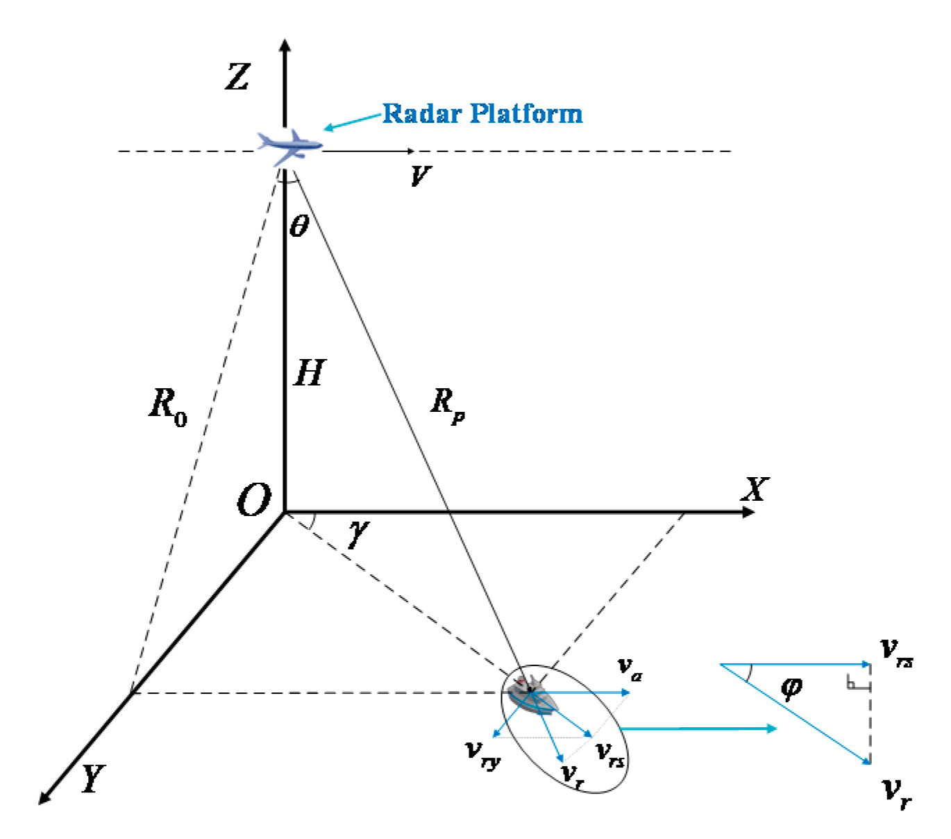
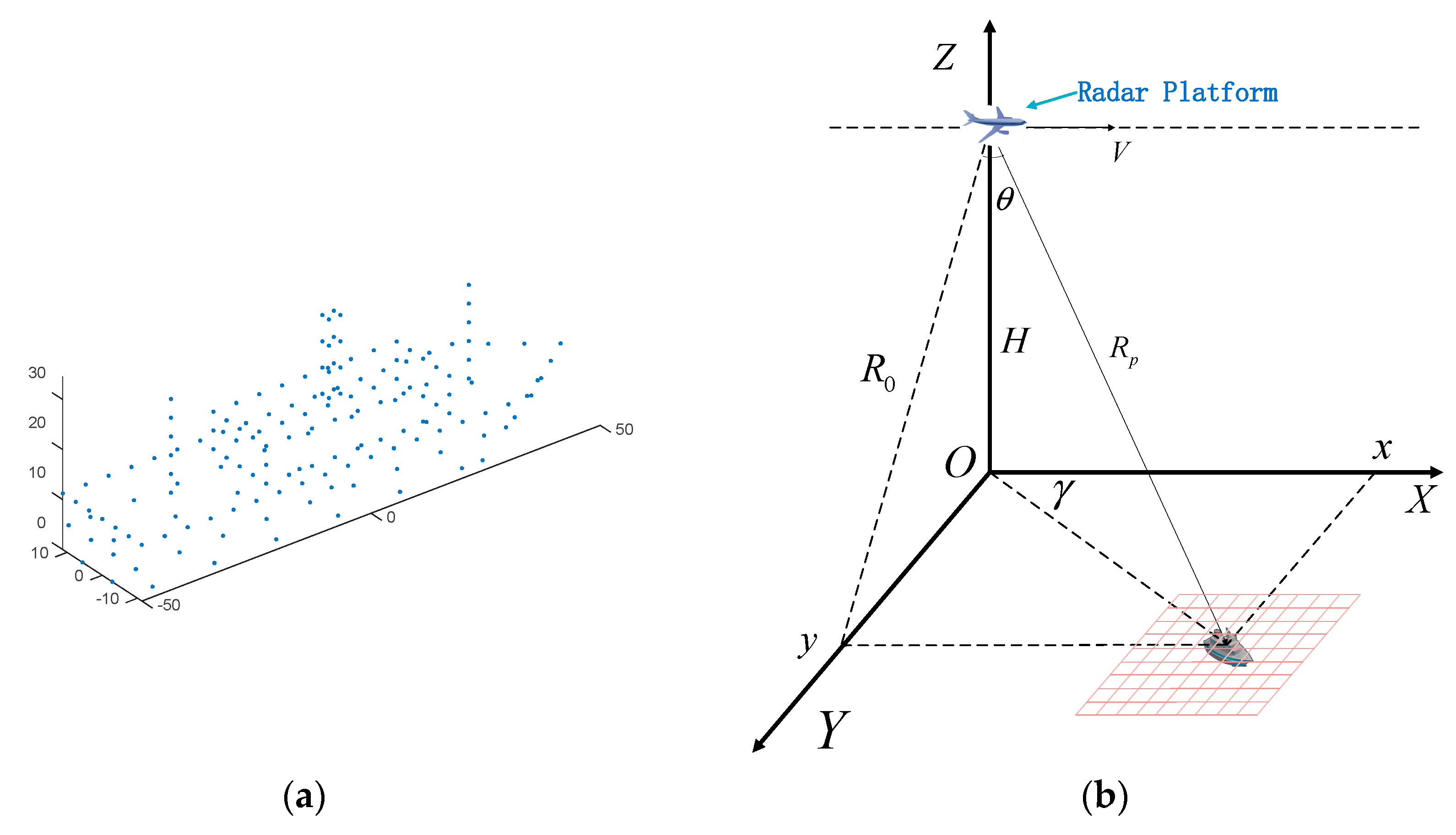
The geometry of a squinted SAR is shown in Figure 1. Define the system of Cartesian coordinates , and assume that a platform with a single-channel radar moves along the X-axis with a constant speed . denotes the squint angle, and indicates the altitude of the platform. The radar position at the azimuth slow time is , where represents the position of the radar antenna phase center (APC).
Suppose that a ship with a constant speed arrives at point exactly at . can be decomposed into and , where denotes the along-track velocity along the horizontal axis and represents the cross-track speed, which is the projection of the radial velocity on the Y-axis. The relationship between and can be written as
Thus, the instantaneous slant range of point is expressed as
This equation can also be expressed as follows [28]:
where represents the relative speed between the ship and the radar and
Based on (3), we can regard a moving target as stationary and focus on it through the estimation of the parameter . Thus, the moving ships can be considered as stationary targets, the position of which is and the sampling interval of which is , where denotes the sampling interval of the initial imaging model, which can be obtained by
Assume that the transmitted signal is linearly modulated in frequency, which can be constructed as
where represents the carrier frequency, denotes the fast time and indicates the chirp rate. The received signal from the target is expressed as
where denotes the pulse width of the transmitted signal, denotes the rectangular function, denotes the target scattering coefficient and represents the synthetic aperture time. Because the instantaneous slant range is known, the signal echoed from point after range compression and demodulation is written as
where and indicate the range envelope and azimuth envelope in the time domain, respectively, denotes the chirp bandwidth and represents the wavelength.
2.2. BP Algorithm
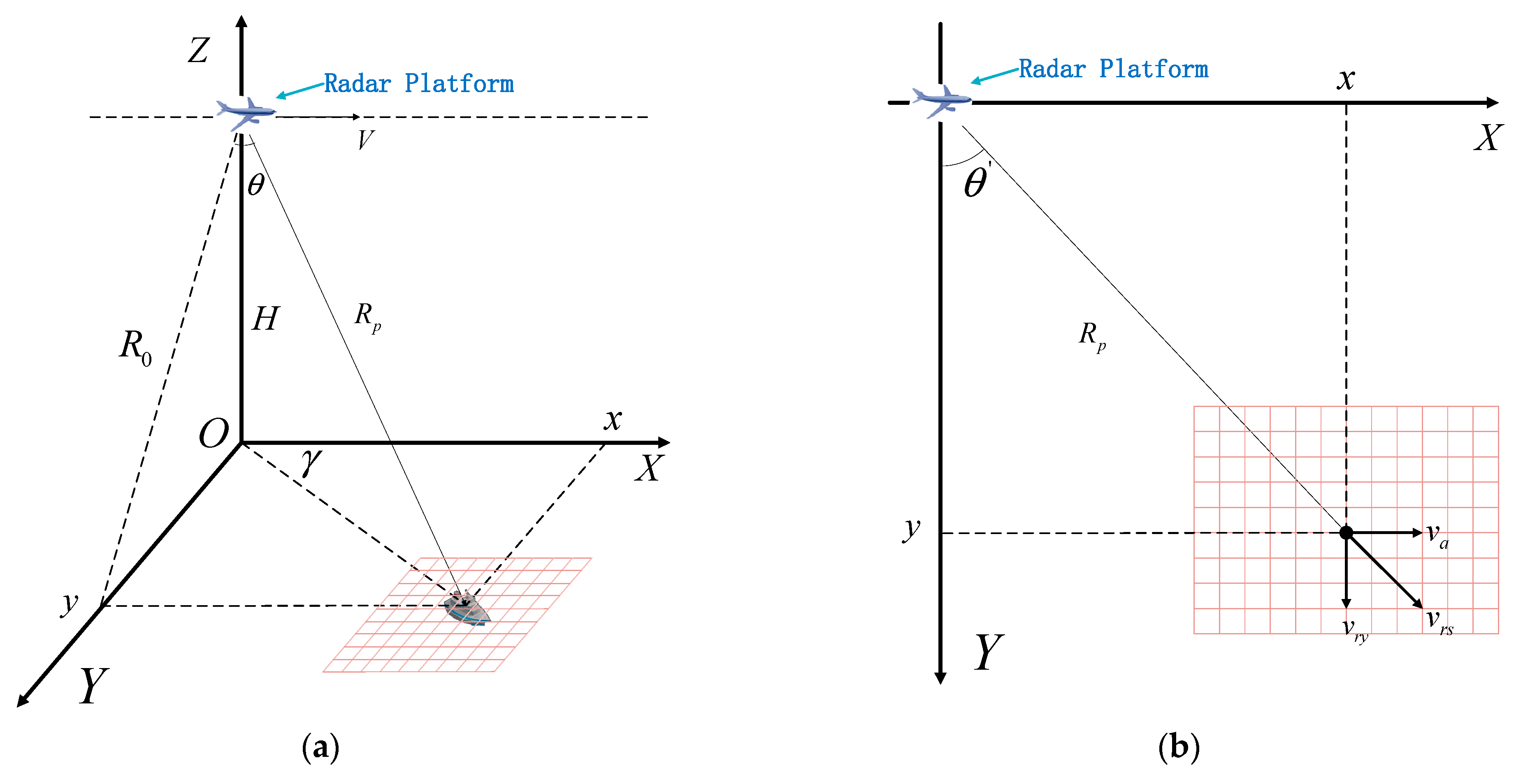
The precise function of the 2-D wavenumber spectrum of a moving target after the BP integral is derived in this section. The BP algorithm is utilized to project the range-compressed data onto a predefined ground grid in the time domain. The exact expression of the data after range-compressing is shown in (9). In this section, the imaging grid is predefined on the ground, as shown in Figure 2a. Figure 2b is a vertical view of the predefined imaging grid.
Assume that the imaging result using BP algorithm is ; then, the BP integral is expressed as
where denotes the amplitude of [17], which is the radar wavenumber, the direction of which is from the radar APC to the moving targets. denotes the range frequency. Since the transmitted signal is a linear frequency-modulated (LFM) signal, as shown in function (7), the range frequency can be expressed as ’. denotes the instantaneous slant range between each imaging grid and the radar beam center, which can be constructed as
and in (10) represents the received signal range compression, which can be obtained by translating the function into the range wavenumber domain, which can be written as
where is the envelope function of the radar wavenumber , which can be written as
where and denotes the length of .
Substituting (11) and (12) into (10), can also be expressed as
where
Because of the ship’s translation, the relative speed factor is not equal to 1. Thus, coherent accumulation cannot be implemented by (14), which results in smearing of the target.
To obtain the residual phase error induced by the translation and estimate the motion parameters, the imagery is translated into the 2-D wavenumber domain, which is given by
where and denote the azimuth wavenumber domain and range wavenumber domains of the BP image, respectively. We substitute (14) into (16) and obtain the following expression:
By calculating (17), we obtain the precise function of the 2-D wavenumber spectrum:
where and represent the range envelope and the azimuth envelope, respectively, in the 2-D wavenumber domain. The detailed derivation of the function is given in Appendix A. In addition, the ship’s position is decided by the first exponential term in (18), although it often deviates from its real location. The second exponential in (18) represents the residual phase error, which can be removed by motion compensation.
2.3. Wavenumber Support Region Analysis
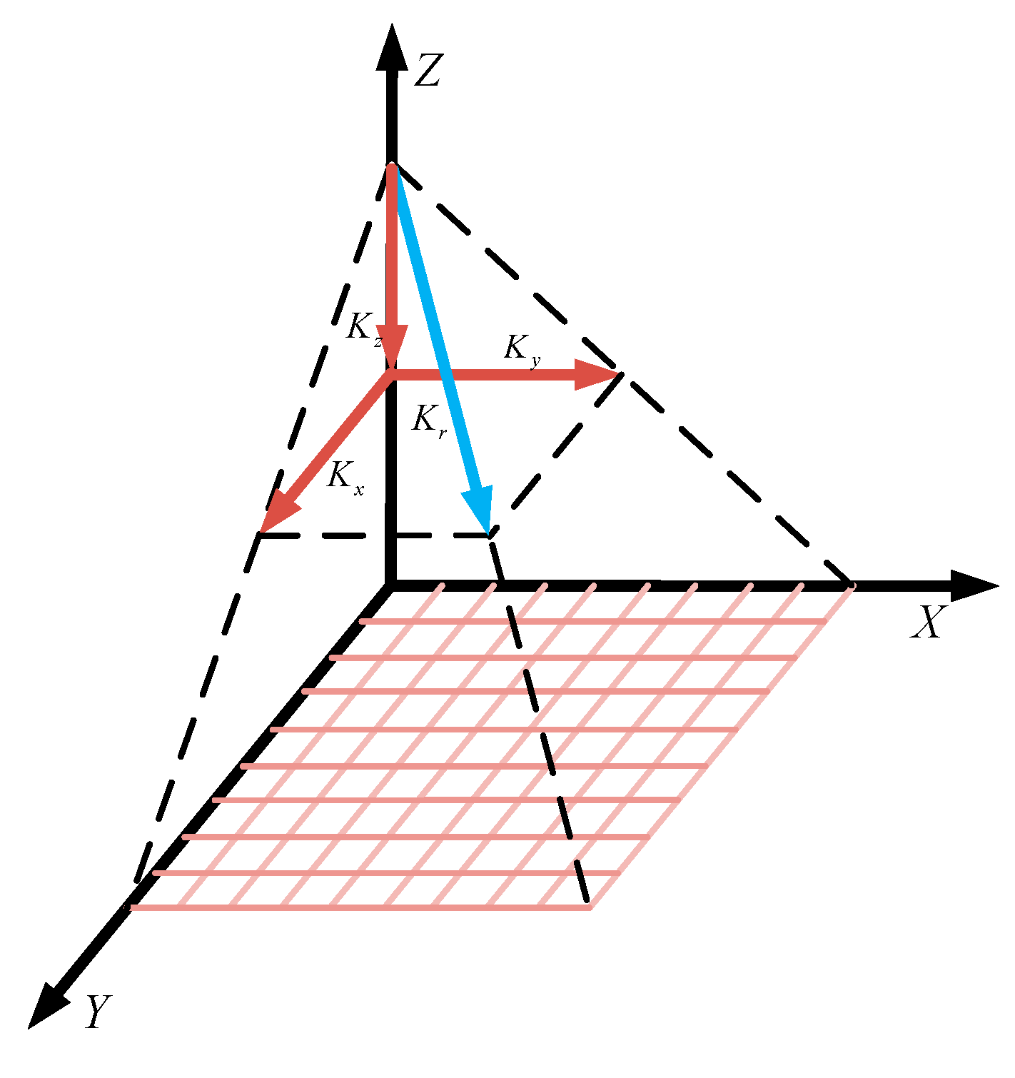
To get the orthometric spectrum, the 2-D wavenumber region needs to be analyzed to obtain the off-centering and inclination features. A schematic diagram of wavenumber decomposition is shown in Figure 3.
is the radar wavenumber. Its magnitude remains constant in the synthetic aperture interval, while its direction varies. It can also be decomposed into three directions , , and . and denote the azimuth wavenumber and range wavenumber, respectively, whose magnitudes at an arbitrary time can be defined as and .
To obtain the wavenumber support region of point at , (17) can also be expressed as
According to (12), the raw data have no relationship with and . Therefore, (19) can be expressed as follows:
Let
Then, the principle of stationary phase (POSP) is applied to (21), after which the support regions of the range wavenumber and the azimuth wavenumber are obtained as follows:
and
Then, the center of the wavenumber support region of each imaging grid can be defined as and , where is the center time of the full aperture. Through functions (22) and (23), and can be written as
and
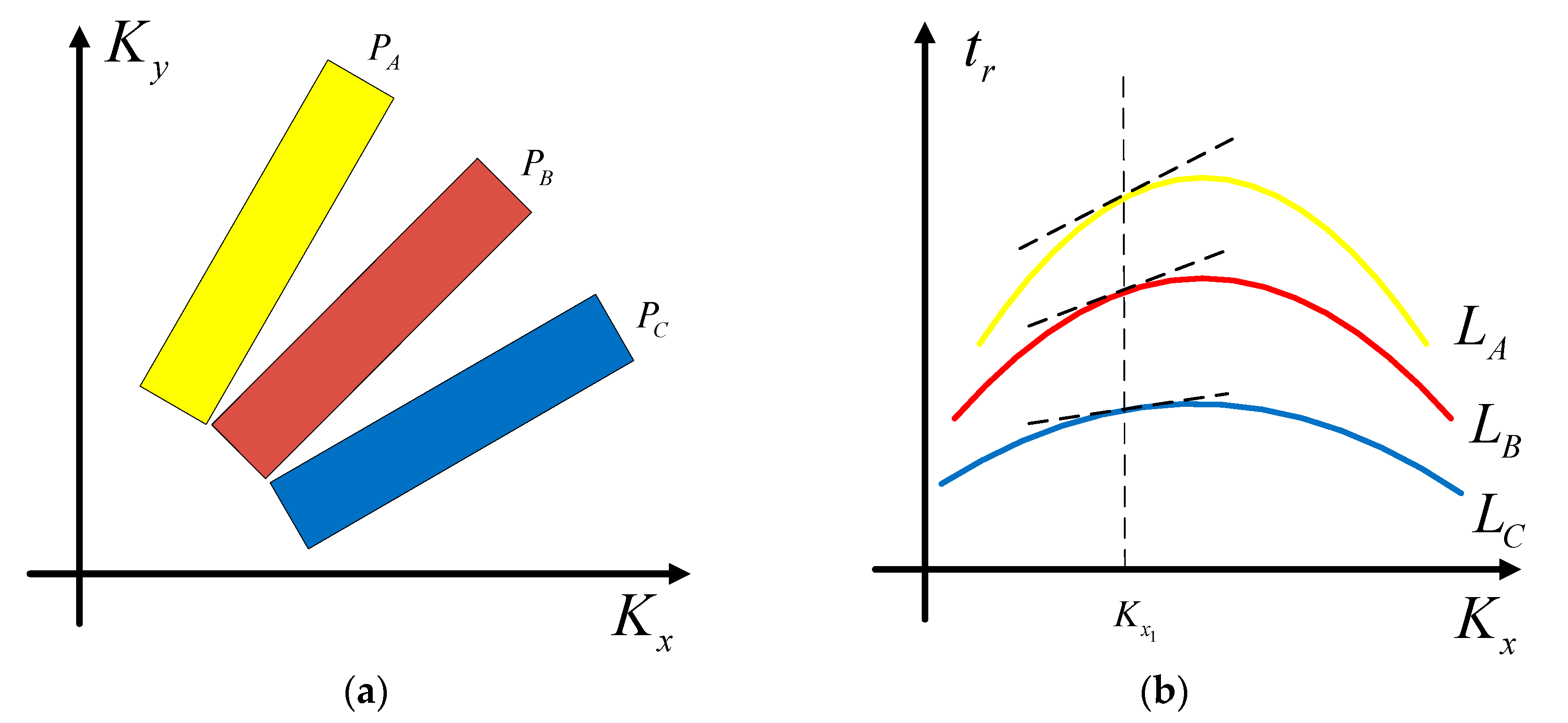
According to (24) and (25), the magnitudes of and have a relationship with the instantaneous slant range . To explain the influence of squinting, a schematic diagram of the wavenumber support region analysis is shown in Figure 4.
Assume that three points in the squint SAR image are obtained by the BP algorithm. The horizontal coordinates and vertical coordinates of the three points are different. In addition, the relationship between them is as follows:
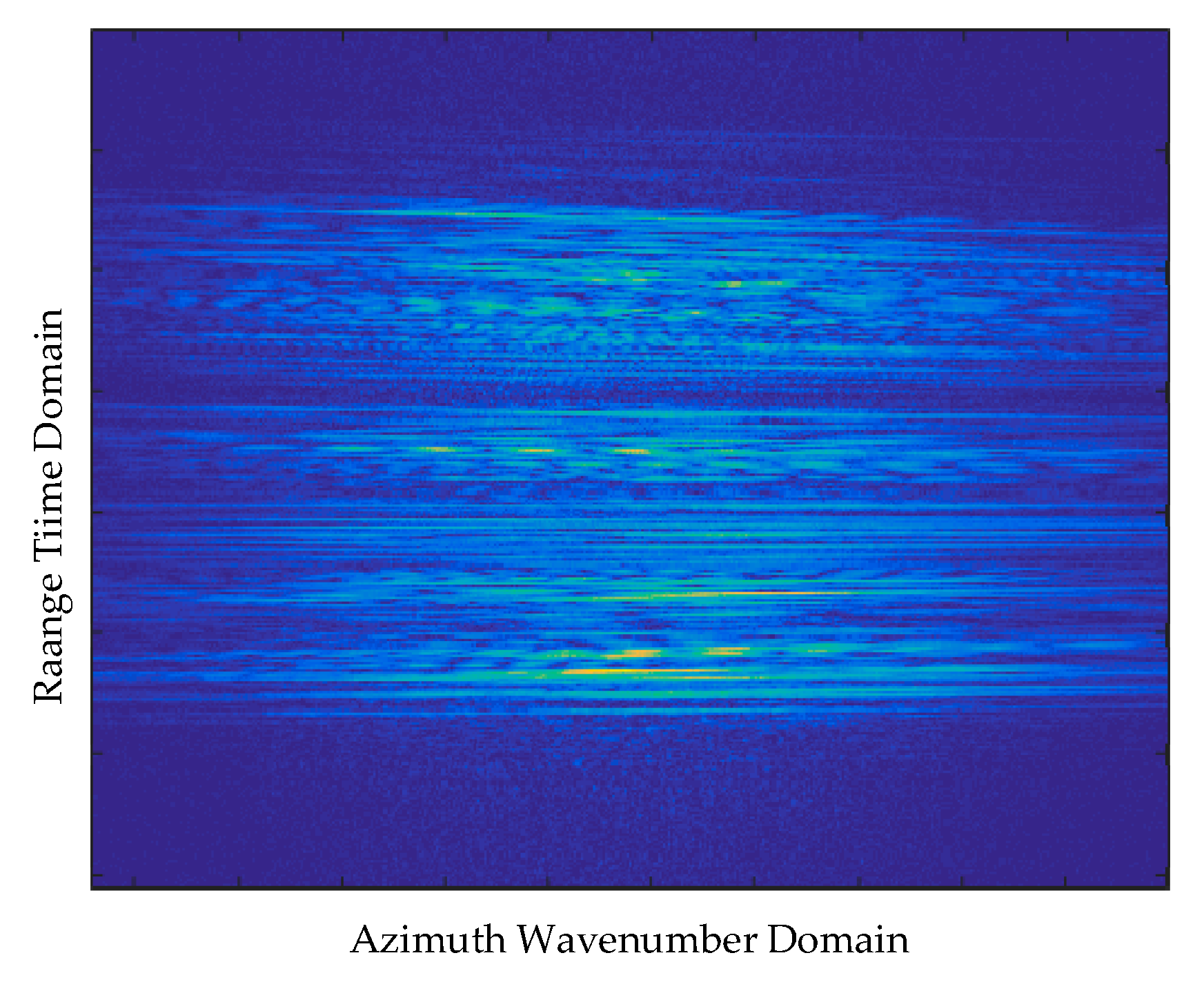
Figure 4a shows the 2-D wavenumber spectrum of the three points. Their support regions are different, which can be clearly seen in Figure 4a. Figure 4 clearly presents two problems. One is that the centers of the three wavenumber spectra are not at the coordinate origin. This will result in the spectrum winding when the support region of the wavenumber spectrum is out of the baseband region. The other problem is that the centerline of each wavenumber spectrum is inclined, which will result in the inclined side lobe of the target in the 2-D time domain. This is the main cause of the geometric deformation. These two problems may result in image spectrum winding and image geometric deformation. Translation of the data into the azimuth wavenumber and range time domains yields the results shown in Figure 4b. , and are the curves of the RCM of the three points in this domain. The gradient of each curve is different at the same azimuth frequency, as shown in Figure 4b. In other words, the curves of the ship data in the azimuth frequency domain will suffer from range space variation. In the case of ship targets or complex sea conditions, this problem cannot be ignored. Figure 5 shows the curves of a moving ship in the azimuth frequency domain obtained from the GaoFen-3 satellite. Clearly, the curvatures of the three curves are different from each other, which will result in considerable difficulty in the processing of motion compensation. Thus, squint minimization is essential in refocusing ships in squint SAR images obtained by BP integrals.
3. The Spectrum-Orthogonalized Refocusing Algorithm
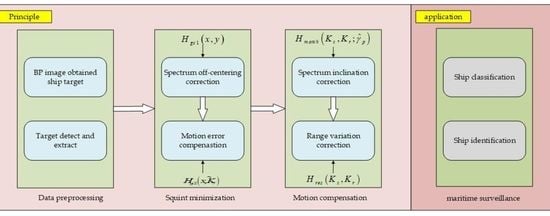
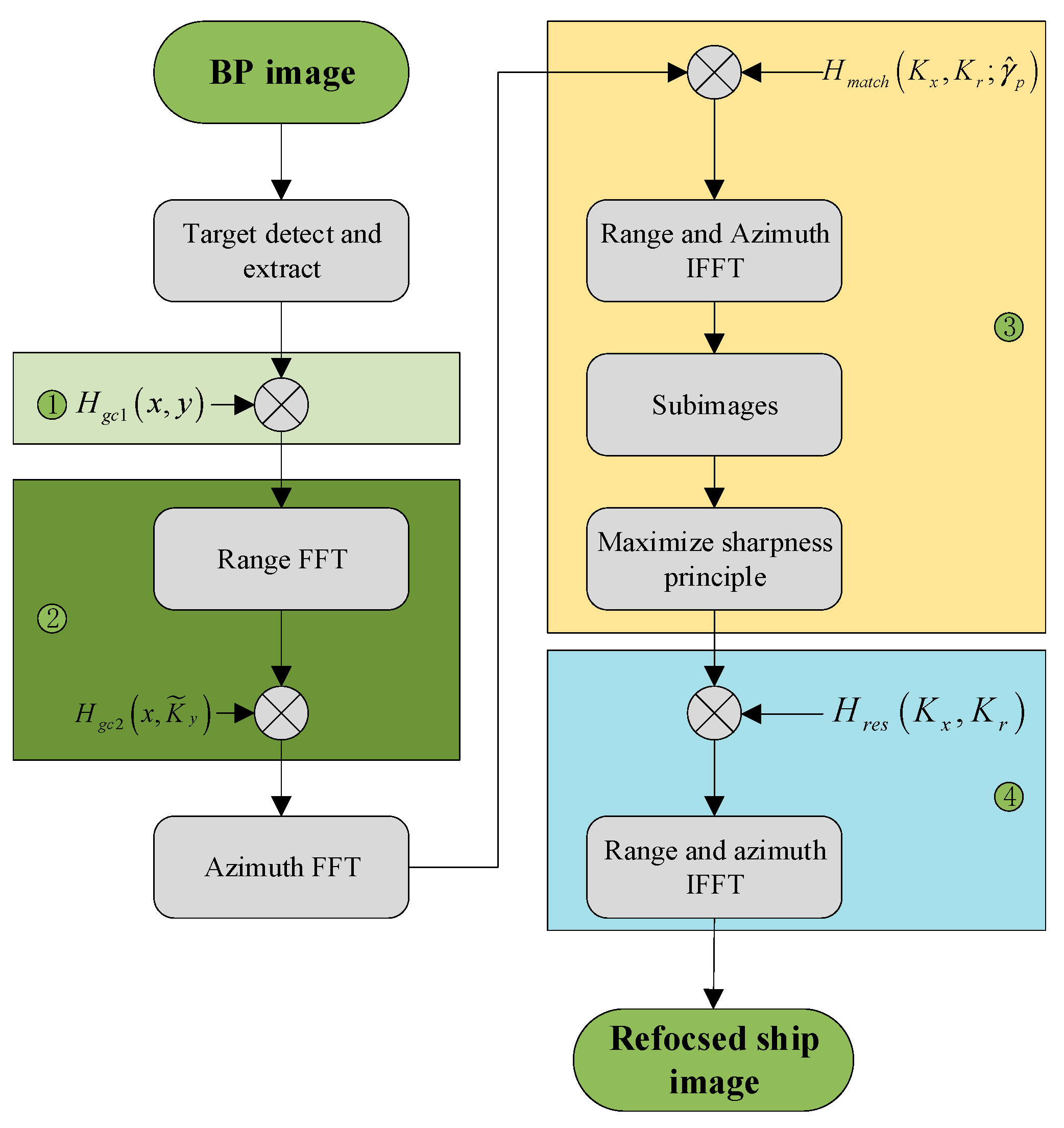
From the previous analysis, the problems of moving ships imaged by BP integrals with squint SAR consist of two main groups. The first group includes image geometric deformation and spectrum winding, which are caused by the spectrum inclination and off-centering, respectively. The second includes smearing of the ship image induced by the translation of the ship. This algorithm introduces a squint minimization method to orthogonalize the spectrum via two-step spectrum compression. The first step of spectrum compression aligns the spectrum centers by moving them to the origin of the coordination. The second step corrects the inclined spectrum by translating it into an orthogonalized form. Finally, to eliminate the effect of the ship’s translation, we derive the function of the 2-D wavenumber spectrum to obtain the motion error caused by translation of the ship. Motion compensation was performed in the 2-D wavenumber domain after the motion parameter was estimated by maximizing the image sharpness. The moving ship was brought into focus when the sharpness of the image is at a maximum. Generally, the flowchart of the squint-orthogonalized refocusing algorithm is as shown in Figure 6.
3.1. Squint Minimization Method
The squint minimization method comprises two steps: the first is proposed to align the off-centering of the spectrum, and the second step is used to calibrate the inclination of the spectrum centerline.
3.1.1. First Step of Squint Minimization for Spectrum Center Alignment
Because the linear phase can induce spectrum movement, we can construct a 2-D compensation function in the time domain to move the spectrum to the coordinate origin, the phase partial derivatives of which are equal to the spectrum offset. The range between each imaging grid and the radar beam center at the center time of the full aperture can be expressed as
The first step of squint minimization can be expressed as
where denotes the image after the first step of squint minimization and denotes the compensation function, which can be written as
denotes the phase of the compensation function and its 2-D partial derivatives are the 2-D spectrum offset, as shown in functions (24) and (25). Substituting (28) into (24) and (25), the partial derivatives of is written as
Then, can be acquired through integrating the partial derivatives as
and
where is a constant without relationships with and . The constant phase error is ignored because it has no effect on ship refocusing. Combining functions (30) and (33), the compensation function can be written as
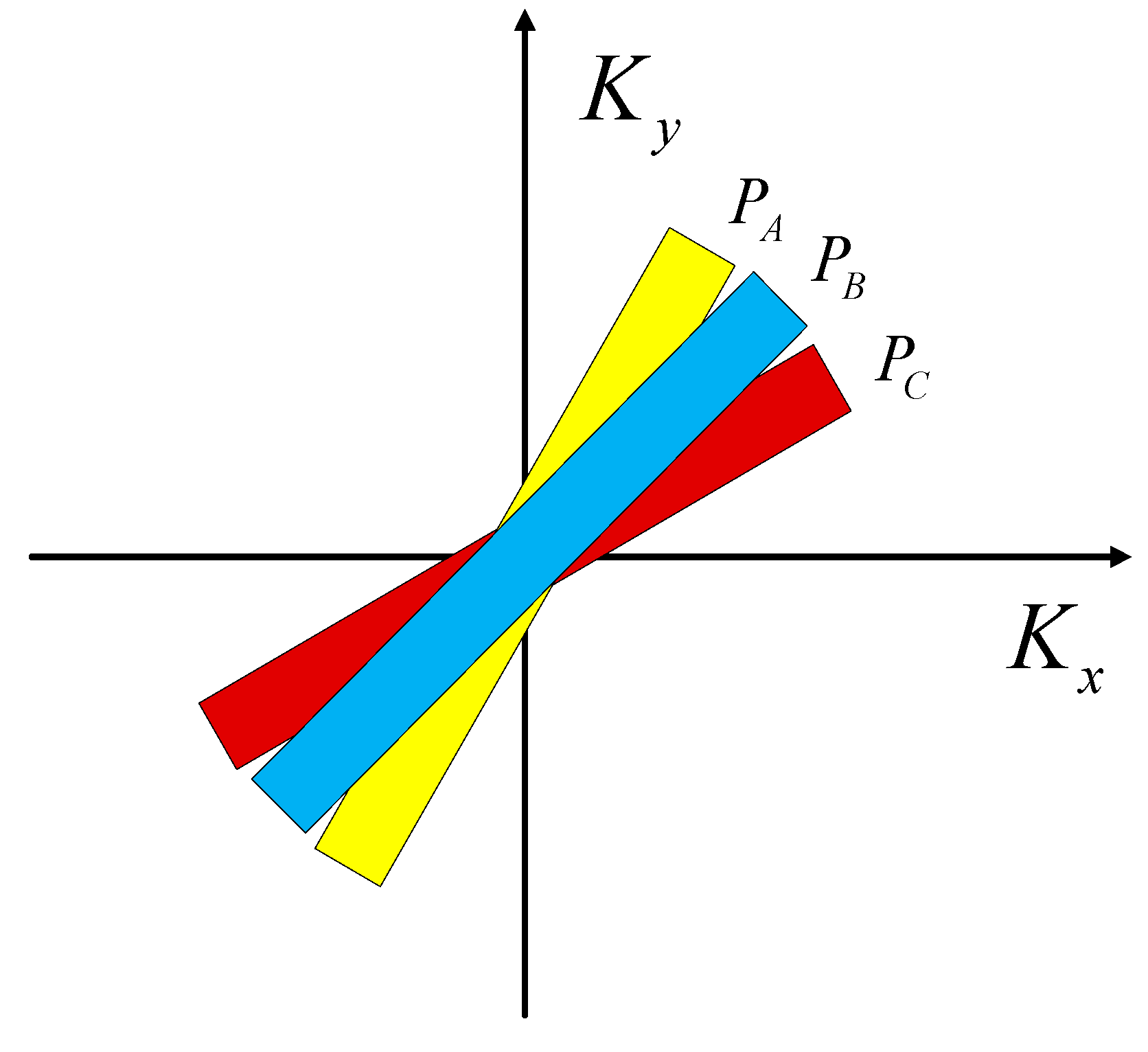
The frequency domain after the compensation is shown in Figure 7. Clearly, the center of each wavenumber spectrum is at the coordinate origin, and the size of the spectrum is obviously reduced. However, the inclination of the 2-D wavenumber spectrum still exists, which can be solved in the second step of squint minimization.
3.1.2. Second Step of Squint Minimization for Spectrum Inclination Correction
After the first step of squint minimization, the off-centering of the 2-D wavenumber spectrum was resolved. In this section, the second step of the squint minimization method is proposed to translate the inclined spectrum into orthogonalized form.
- (1)
- Illustration of the second step of squint minimization
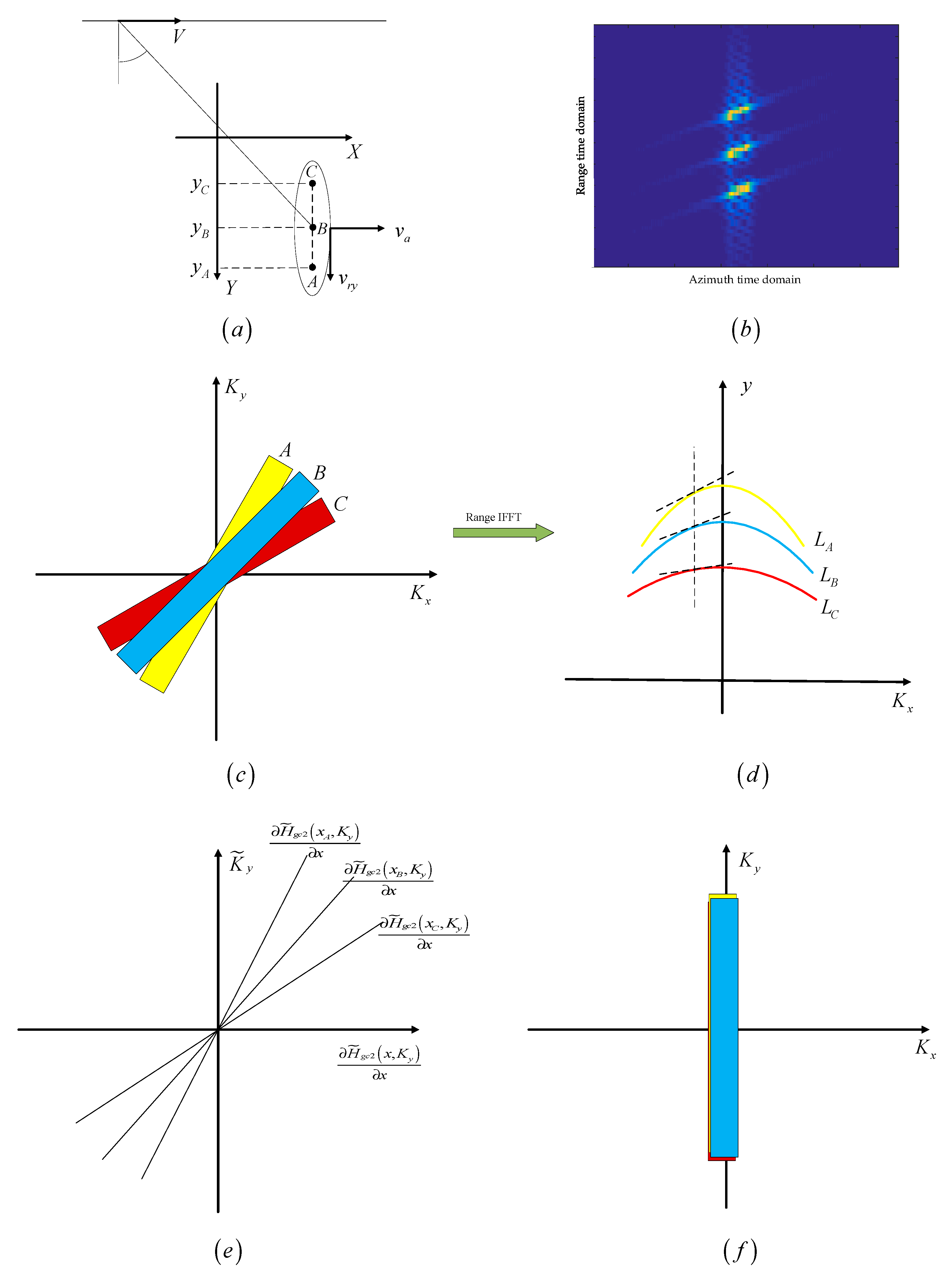
Assume that three points are located in the same azimuth bin, signed as A, B, and C. As shown in Figure 8a, the vertical coordinates of the three points are , , , respectively, and the relationship between them is given by
Figure 8b presents the imaging results of the three points obtained by the BP algorithm. The side lobe of each point target is oblique, which increases the coupling of the range and the azimuth in the 2D wavenumber domain. The 2D wavenumber spectra of the three targets are shown in Figure 8c. The off-centering of the spectrum has clearly been removed after the first step of geometric correction. The curves of the RCM are given in the azimuth wavenumber and range time domains, which is shown in Figure 8d. The RCM curves of the three points have different gradients at the same azimuth frequency. This problem means that the RCM response curves will not cohere with each other, which limits the effectiveness of the unified range cell migration correction (RCMC). An original spectrum compression function in the range wavenumber domain is presented to solve this problem, which is shown in Figure 8e, and is used to correct the wavenumber spectrum inclination. Thus, the partial derivative with respect to the azimuth direction of the compression function is equal to the gradient of the wavenumber support region centerline. Figure 8 illustrates the second step of geometric correction. The inclination of the wavenumber spectrum is removed after the correction, as shown in Figure 8f.
- (2)
- Derivation of the second step of squint minimization
Through (24) and (25), the centerline of each imaging grid after the first step of squint minimization can be expressed as
Let and ; the centerline of the wavenumber support region can be written as
In this paper, we refocus a moving ship in the ROI data extracted from a rough image. The value range of is determined by the size of the ship target. The azimuth spectrum expansion varies with and is neglected since only a small image containing a moving ship is extracted from the rough image. Thus, let denote the middle of the data range; the wavenumber support region centerline can thus be rewritten as
The second step of squint minimization can be expressed as
where denotes the image after the first step of squint minimization and denotes the compensation function, which can be written as
denotes the phase of the compensation function. Since the partial derivative of the spectrum compression function relative to is equal to the wavenumber support region centerline, the partial derivatives of relative to can be written as
Then, can be obtained by integrating the partial derivatives as
Thus, the compensation function of the second step can be expressed as
According to (40), we can correct the inclination of the 2-D wavenumber spectrum and remove its cross-range-dependent RCM.
3.1.3. Computational Complexity of the Squint Minimization Process
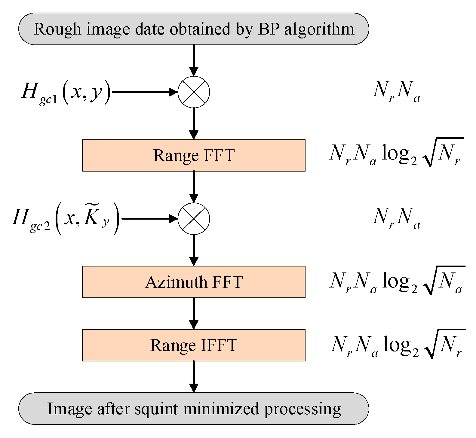
Assume that the size of a scene containing a moving ship is . Thus, the computational load of the squint minimization process is as shown in Figure 9.
Because many pieces of hardware and software are used for FFT acceleration in practical engineering applications, the FFT is dozens or even hundreds of times faster than interpolation under the same computational load. For example, only 0.7 s is required when applying FFT to a matrix of 10,000 × 10,000 in MATLAB, while the sinc-interaction takes 16 s. Thus, since the presented method involves no interpolation and can be implemented by the FFT and IFFT, it is much more computationally efficient than the interpolation class refocusing algorithm, such as that presented in [27,30]. Because the presented algorithm needs approximately three iterations to estimate the motion parameters, its computational efficiency is less than that of some classic refocusing algorithms, which contain no interpolation or iteration, such as the PGA algorithm. Since the method uses the ROI data to refocus moving ships, the difference in computational complexity is small.
3.2. Motion Compensation via the Relative Velocity Estimation
Since the residual phase error caused by the translation of ships leads to smearing of the imaging result based on the BP algorithm, the phase error has to be eliminated by motion compensation. Motion compensation is implemented in the 2-D wavenumber domain by removing the third exponential term in (18). To do this, we need to obtain the location of the moving ship in the SAR image and the relative velocity . Since the ship can be divided into many scattering points, the coordinates of its geometric center can represent its position in an SAR image if the ship is small enough. Then, the relative speed can be estimated through the maximum sharpness. First, since the relative speed is defined as
by roughly estimating the speed range of the ship, we can define the value range of by referring to function (45). Through function (18), the coarse compensation function can be constructed as
After coarse compensation, the coarse imaging result of the ship can be expressed as
where
Since the quality of the image strongly depends on the accuracy of , the maximizing sharpness principle is applied to precisely estimate the parameter . This principle can be expressed as
where denotes the coarse imaging result in the time domain. To obtain the parameter , the method proposed in [34] is used to solve function (49). After is acquired, we can multiply (18) by (46) to remove the residual phase. However, if the size of a ship in the SAR image exceeds that of a range cell, the range space variation of the residual phase error cannot be neglected. Assume that another point exists on the ship, whose position after BP imaging is , where . Thus, the exact compensation function for motion compensation is expressed as
However, the function used for motion compensation is (46). Thus, the residual motion error of this point can be expressed as
The moving ship can thus be refocused well by this motion compensation.
4. Simulation and Real Data Results
In this section, data processing of the results of the simulation experiments and GaoFen-3 squint SAR data processing were performed to validate the effectiveness of the squint minimization refocusing algorithm.
4.1. The Simulation Results for a Ship Target
The simulation uses a point target array to represent the ship target. As shown in Figure 10a, the ship’s 3D geometry in this simulation consists of 177 scatters, which are settled in a sense, as shown in Figure 10b. The size of the scene is 40 m × 100 m. It is divided into 100,000 grids, each of which is 20 cm × 20 cm. The squint angle of the transmitted signal is 30°. The ship target has an azimuth velocity of 3 m/s and a cross-azimuth velocity of 1 m/s. The radar parameters are shown in Table 1.
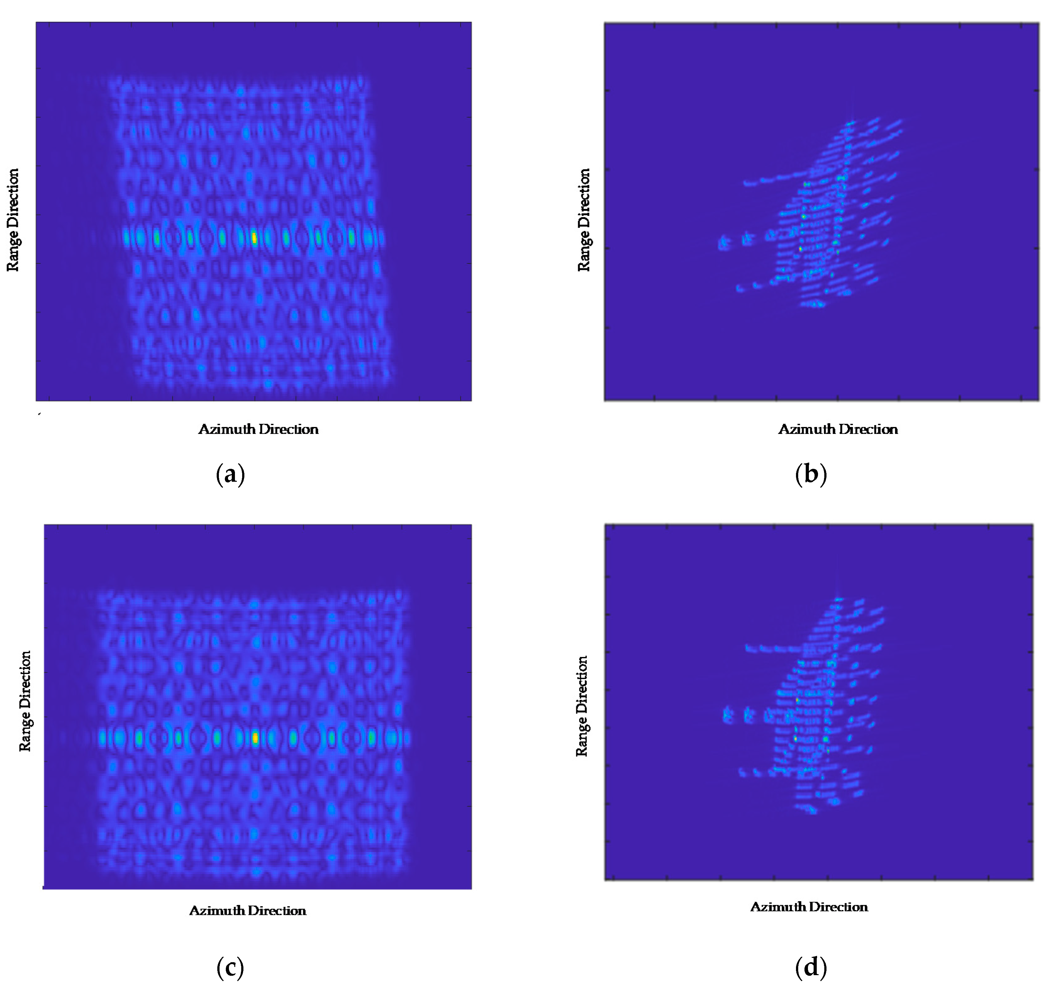
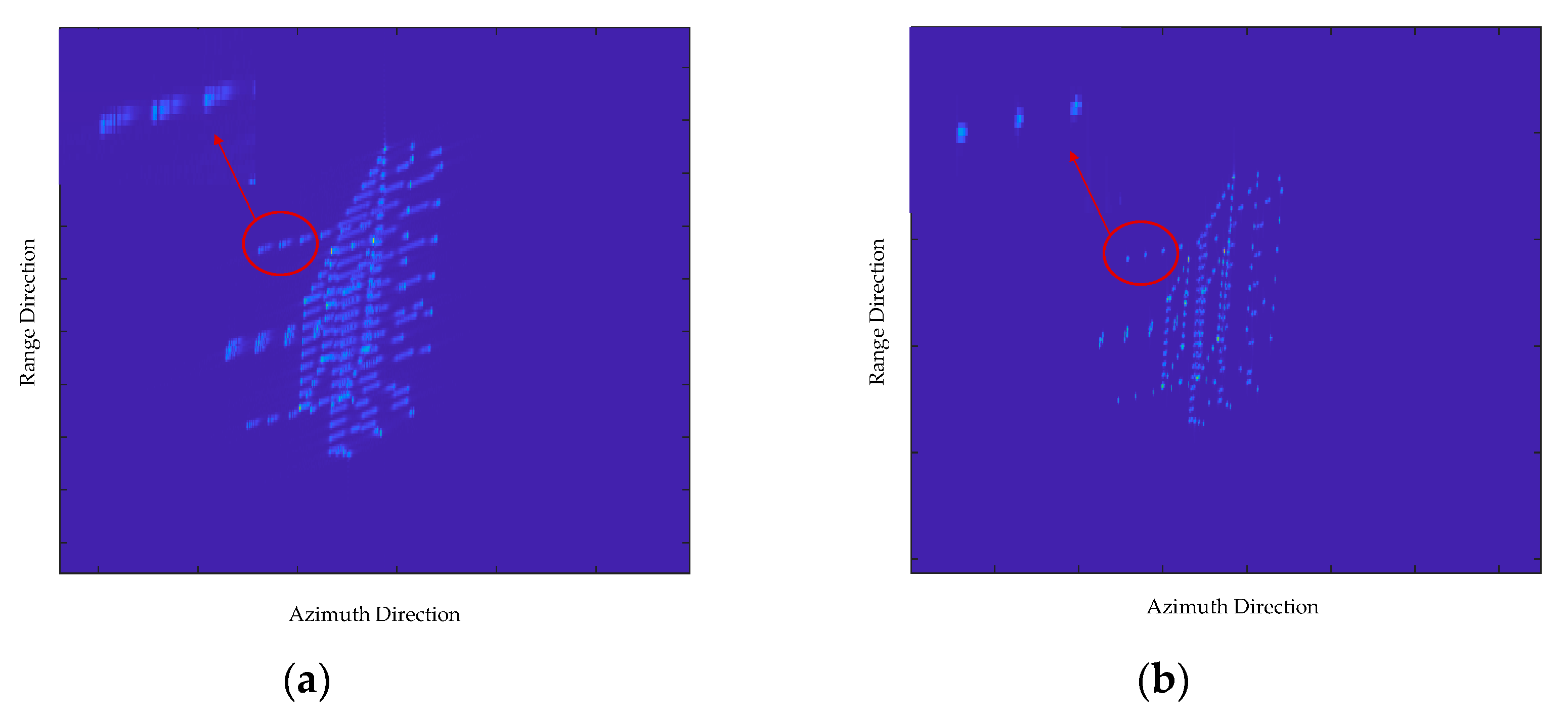
Figure 11a shows the wavenumber spectrum of a rough image. Figure 11b is a rough image of the ship obtained via the BP algorithm. The energy of the simulated ship target spreads along an oblique direction due to the spectrum inclination. Figure 11c shows the wavenumber spectrum of the image after squint minimization. Clearly, the inclination of the spectrum is corrected after squint minimization. Figure 11d is the image after squint minimization. The side lobes of the range and the azimuth are clearly orthometric, which will reduce the coupling of the range and the azimuth in both the time and frequency domains, thus facilitating the parameter estimation and motion compensation processes. Figure 12 shows a comparison with the PGA algorithm. Figure 12a shows the result obtained by the PGA algorithm. Figure 12b shows the result obtained via the presented algorithm. As shown, the result obtained via the presented algorithm is clearer than the result obtained via the PGA algorithm. In addition, we magnified three highlight points in the red circle and can see that the points obtained via the proposed algorithm are focused better than the other one. There are still many energies spread along the side lobe, which can be seen visualized in Figure 12. The simulation result indicates the effectiveness of the presented method.
4.2. Real Data Results
Real experimental data recorded by the GaoFen-3 satellite were obtained to assess the performance of the presented refocusing method. A C-band (5.4 GHz) SAR was installed on the GaoFen-3 satellite launched by China in August 2016 [35,36,37,38,39]. The SAR images of three moving ships obtained by the BP integral were chosen for this experiment. The synthetic aperture time to the image target was short enough so that the effective rotation of the target could be regarded as constant. The image contrast [40] and entropy [19] of the image intensity were used to compare the imaging results.
4.2.1. The Imaging Result of Ship NO.1
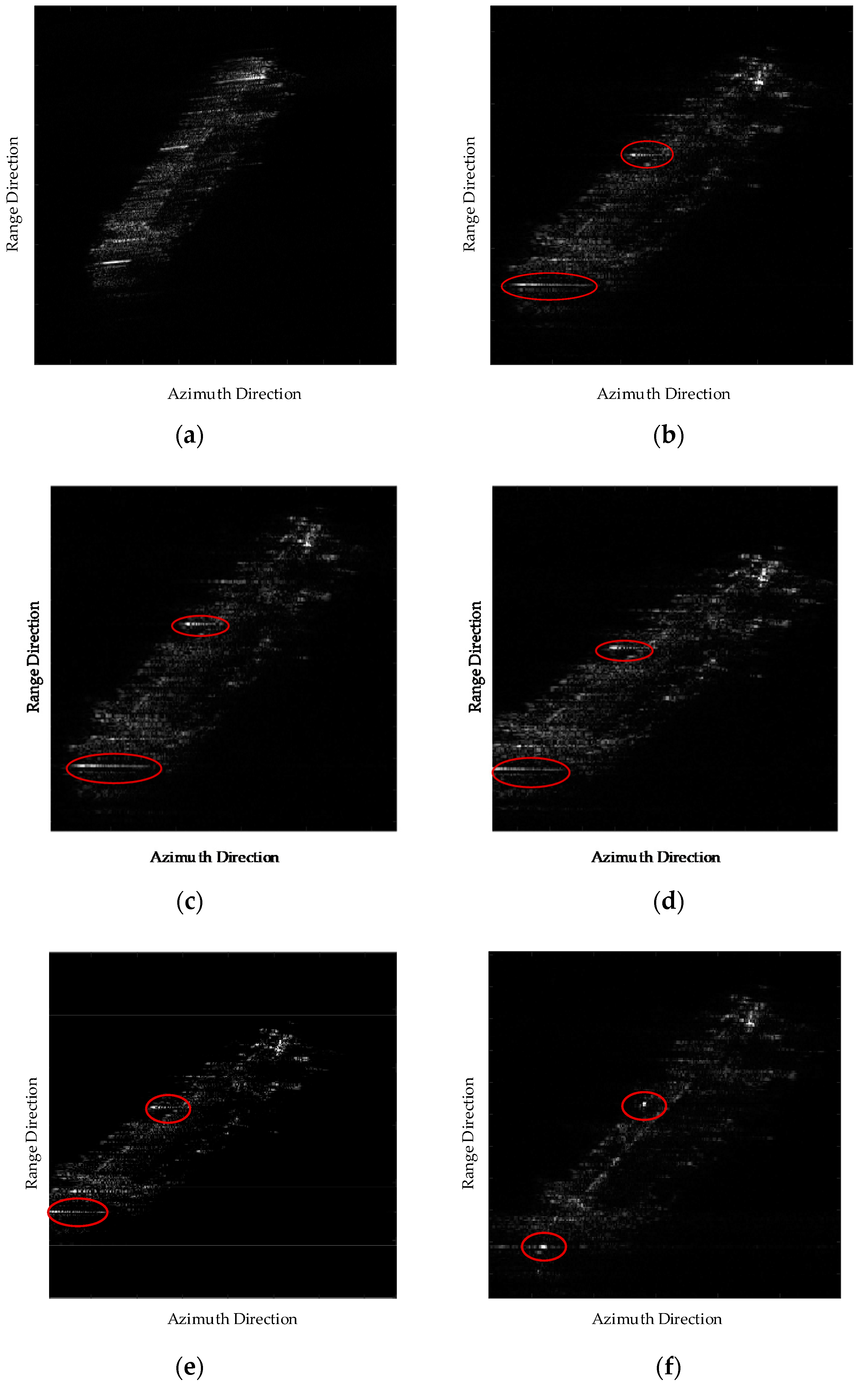
The rough image of the ship collected by the GaoFen-3 satellite through the BP integral in the squint model is smeared, as shown in Figure 13a. The side lobe is inclined because of the spectrum inclination. Thus, the moving ship is difficult to refocus within the synthetic aperture time. Figure 13b–f shows the results of refocusing the ship in the squint SAR image before squint minimization via the PGA, the compressed sensing-based ISAR (CS-ISAR) imaging algorithm, the Doppler parameter estimation algorithm (DPEA) [26], the back-projection sub-image autofocus (BPSA) algorithm [30] and the method presented in this work, respectively. The ship’s contour in Figure 13f is delineated more than the results in Figure 13b–e because the spectrum inclination is not removed by the other four algorithms. The image contrast and entropy results are shown in Table 2. The CS-ISAR algorithm uses a compressive sensing-based method to process the SAR date after motion compensation with classical ISAR technology, which can improve the resolution of the imagery. Thus, this method performs better than PGA as shown in Table 2. Clearly, the image obtained by the proposed algorithm has lower entropy and higher contrast. A detail of the highlight points in the red circle clarifies that Figure 13f is better focused than the others. The energy of the highlight points is distributed along the azimuth direction, which can be seen in Figure 13b–e. The azimuth side lobes of the highlight points are much lower than those in Figure 13b–e. Generally, only the driver’s cabin is in focus in Figure 13b–e, whereas in Figure 13f the whole ship is smeared. In addition, compared with the CS-ISAR and BPSA algorithms, the proposed method has higher computationally efficient and its computational load is close to those of the PGA and DPEA algorithms.
4.2.2. The Imaging Result of Ship NO.2
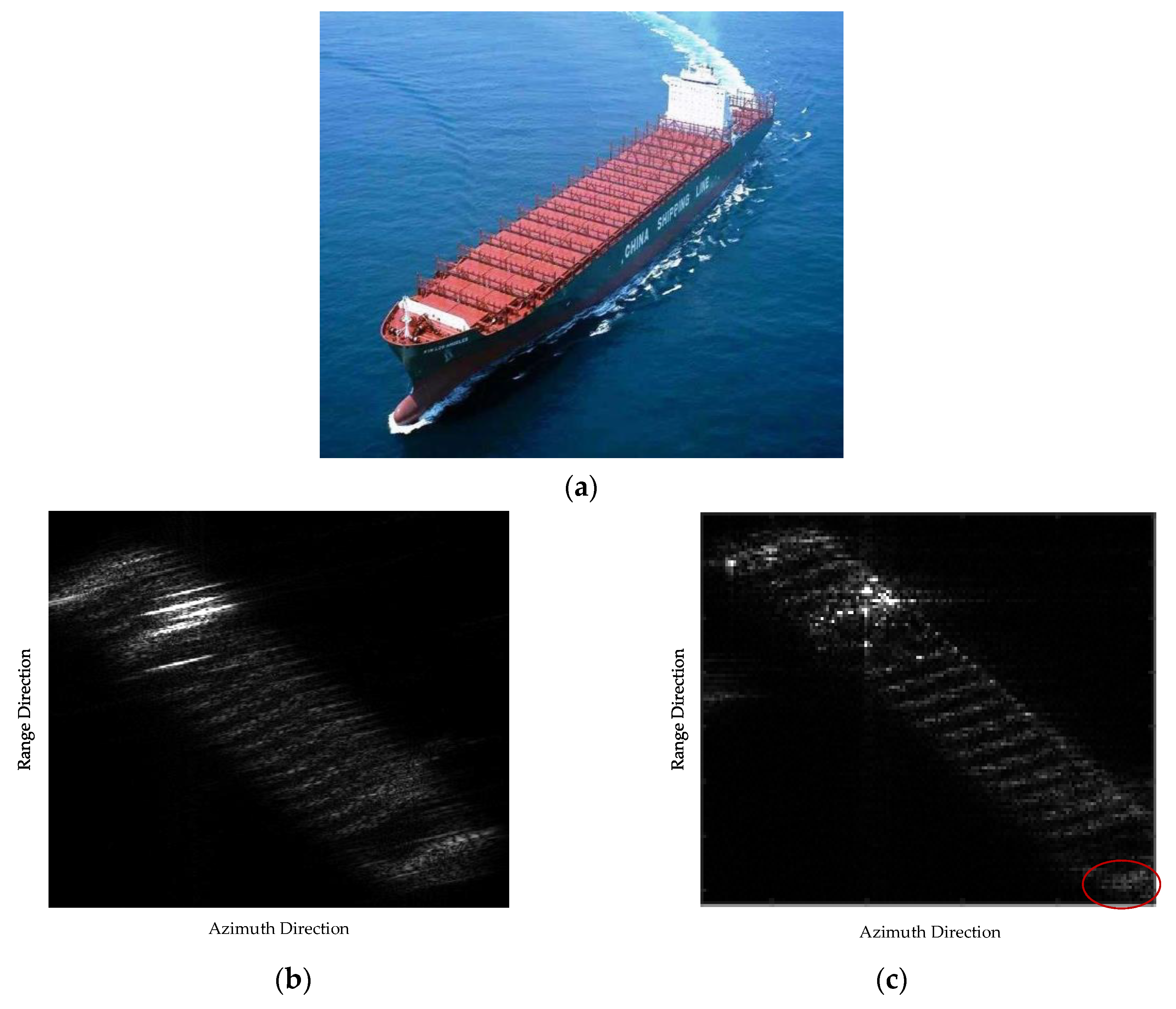
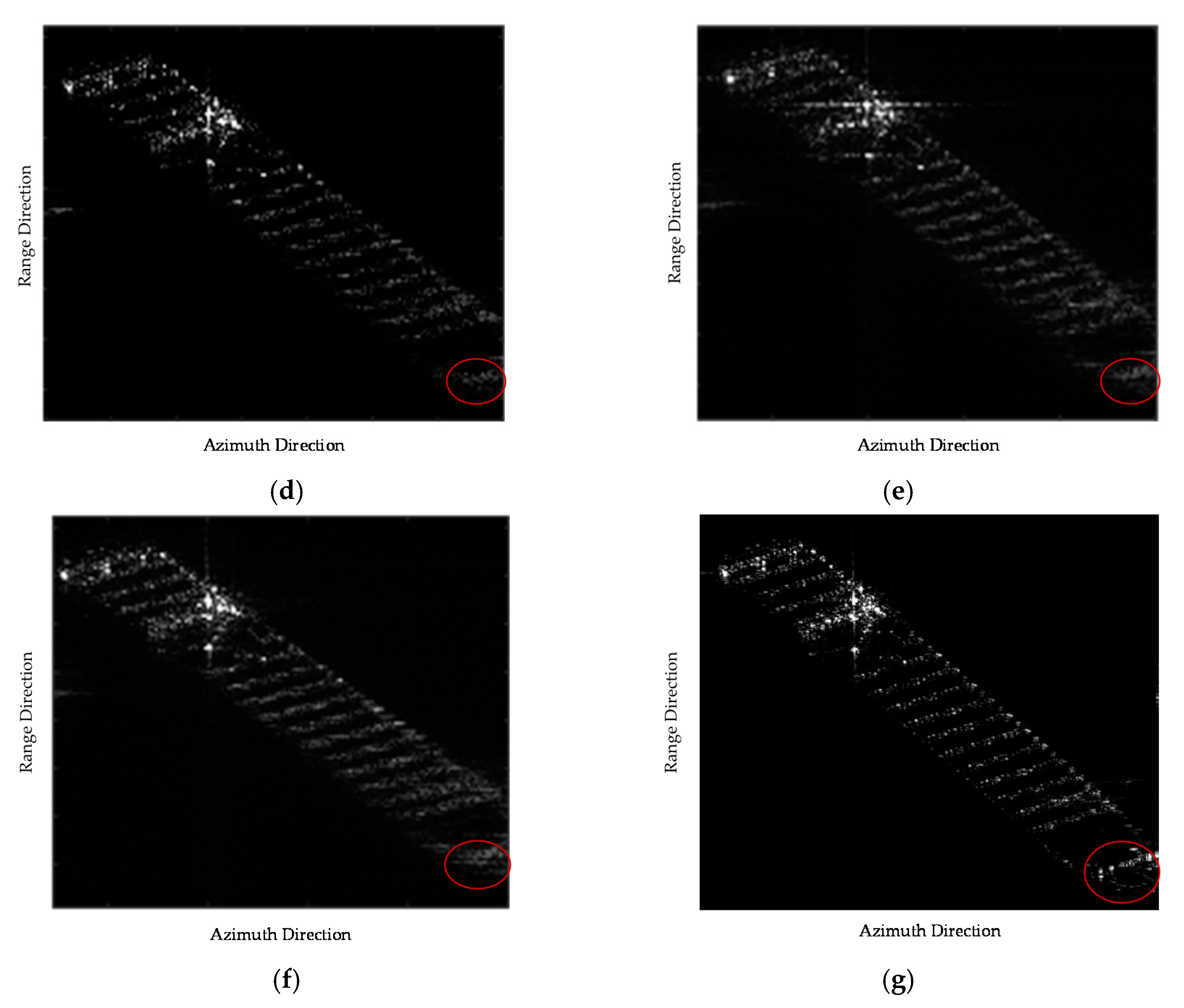
The optical image of a tanker is shown in Figure 14a,b shows the GaoFen-3 squint SAR image of the tanker. Figure 14c–g shows the refocusing results of the ship in the squint SAR image before squint minimization via the PGA, the CS-ISAR, the DPEA [26], the BPSA [30] and the method presented in this work, respectively. However, the GaoFen-3 squint SAR image of the tanker experiences more serious defocusing than that experienced by the two ships above. The quality of the refocusing image in Figure 14c obtained via the proposed algorithm is greatly improved when compared to that of the GaoFen-3 squint SAR image in Figure 14b. Table 3 presents the image parameters of Figure 14c–g. It can be seen that Figure 14c has a smaller entropy and higher contrast than the images shown in Figure 14c–g. From a visual point of view, only Figure 14g is well focused, because the details of the deck are only visible here. All of the decks in Figure 14b–f are out of focus. Especially the points in the red circles, Figure 14b–f are smeared and there is no focused point in the circle. Only the deck in Figure 14g is almost focused. Generally, these results indicate that the proposed algorithm performs better in the case of squint SAR. Therefore, the refocusing result verifies the effectiveness of the proposed method.
5. Discussion
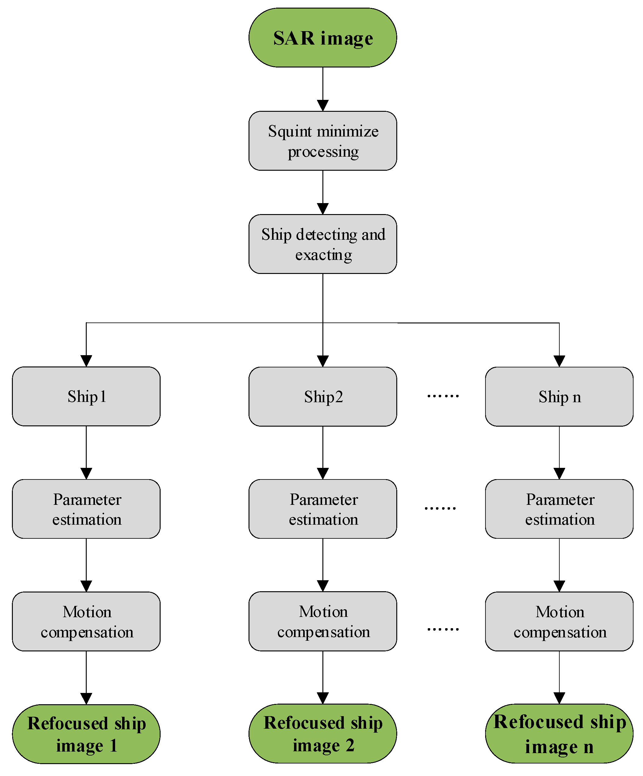
In this section, the validity of the proposed method in the case of multiple moving targets in a large scene is discussed. In this case, we can perform the squint minimization process on the whole rough image. The geometric deformation of all multiple moving targets will be corrected after the processing. Then, we detect and extract every ship target in order to remove the motion errors of each target. Finally, motion parameters estimation and motion compensation are performed for each target. The flowchart of the squint-minimized-based refocusing algorithm for multiple moving ships in a large scene is shown in Figure 15.
The proposed method requires a short synthetic aperture time because the procedure for the motion compensation contains a constant velocity of the target. Thus, the method is not suitable for a long synthetic aperture time and complex sea conditions. In addition, the shaking of the moving ship will influence the imaging result of the proposed method in complex sea conditions. This is also a huge challenge nowadays. Thus, refocusing moving ships in such cases will be an important research topic in the future.
6. Conclusions
Moving ships in squint SAR images obtained by the BP algorithm usually suffer from spectrum winding and inclination. These problems necessitate refocusing of the squint SAR images of moving ships obtained through a BP integral. To solve the above two problems, this paper presented a new algorithm called “squint minimization” to orthogonalize the spectrum. It uses two spectrum compression functions to correct the spectrum. The first aligns the spectrum centers by moving them to the origin of the coordinate system. The second corrects the inclined spectrum by translating it into an orthogonalized form. Finally, motion compensation is performed in the 2-D wavenumber domain after the relative velocity is estimated by maximizing the image sharpness. The advantages of this proposed method are summarized as follows: (1) it uses a new method called “squint minimization” to orthogonalize the spectrum, which can help to effectively reduce the influence of squinting; (2) it has lower computational complexity because of the lack of interpolation; (3) because the residual motion error caused by the translation is exactly determined without any approximation, the presented method of motion compensation in this paper can also be applied for the refocusing of moving targets imaged by any other SAR imaging algorithm; (4) this algorithm is also valid for multiple moving targets in a large scene. In this case, we can perform squint minimization on the whole rough image. The geometric deformation of all moving targets is corrected after the processing. Then, the CFAR algorithm is utilized to detect and extract every ship target from the scene. Finally, moving ships are refocused after their relative velocities are estimated via the maximum sharpness principle. Owing to these advantages, the presented algorithm has significant potential for application in target detection and classification. Since this method requires a short coherent accumulation time and a moving ship with constant velocity, future work may take the accelerated velocity into consideration, which is also a great challenge for ship refocusing technology.
Author Contributions
Formula analysis, X.T., M.B., G.S., M.X. and L.H.; methodology, X.T.; writing—original draft preparation, X.T.; writing—review and editing, X.T., L.H. and G.S.; supervision, Y.Z.; All authors have read and agreed to the published version of the manuscript.
Funding
This research was supported by the National Science Fund for Distinguished Young Scholars (Grant No. 61825105), the Key Scientific and Technological Innovation Team Foundation of Shannxi (Grant No. 2019TD-002) and the National Natural Science Foundation of China (Grant Nos. 61901346 and 61901348).
Institutional Review Board Statement
Not applicable.
Informed Consent Statement
Not applicable.
Data Availability Statement
Not applicable.
Acknowledgments
The authors thank all the anonymous reviewers for their valuable comments, which helped to improve the quality of this manuscript.
Conflicts of Interest
The authors declare no conflict of interest.
Appendix A
This appendix provides the detailed derivation of function (18). We first translate the range direction of the image into the direction of the vector . Then, we can obtain
We construct the following equation:
where
where . As indicated in function (14), and are constructed as
Translating and into the azimuth wavenumber domain, the two functions are constructed as
Function (A2) can be rewritten as
For , we can obtain the azimuth wavenumber spectrum
By analyzing functions (A5)–(A8), the precise analytic expression of the 2-D wavenumber spectrum is as follows:
References
- Zhang, X.; Liao, G.; Zhu, S.; Gao, Y.; Xu, J. Geometry-information-aided efficient motion parameter estimation for moving-target imaging and location. IEEE Geosci. Remote Sens. Lett. 2015, 12, 155–159. [Google Scholar] [CrossRef]
- Chen, J.; Xing, M.; Xia, X.; Zhang, J.; Liang, B.; Yang, D. SVD-Based Ambiguity Function Analysis for Nonlinear Trajectory SAR. IEEE Trans. Geosci. Remote Sens. 2020, 59, 3072–3087. [Google Scholar] [CrossRef]
- An, D.; Huang, X.; Jin, T.; Zhou, Z. Extended nonlinear chirp scaling algorithm for high-resolution highly squint SAR data focusing. IEEE Trans. Geosci. Remote Sens. 2012, 50, 3595–3609. [Google Scholar] [CrossRef]
- Davidson, G.W.; Cumming, I.G.; Ito, M.R. A chirp scaling approach for processing squint mode SAR data. IEEE Trans. Aerosp. Electron. Syst. 1996, 32, 121–133. [Google Scholar] [CrossRef]
- Xiong, Y.; Liang, B.; Yu, H.; Chen, J.; Jin, Y.; Xing, M. Processing of Bistatic SAR Data With Nonlinear Trajectory Using a Controlled-SVD Algorithm. IEEE J. Sel. Top. Appl. Earth Obs. Remote. Sens. 2021, 14, 5750–5759. [Google Scholar] [CrossRef]
- Chen, J.; Zhang, J.; Jin, Y.; Yu, H.; Liang, B.; Yang, D. Real-Time Processing of Spaceborne SAR Data With Nonlinear Trajectory Based on Variable PRF. IEEE Trans. Geosci. Remote Sens. 2021, 1–12. [Google Scholar] [CrossRef]
- Li, Z.; Xing, M.; Liang, Y.; Gao, Y.; Chen, J.; Huai, Y.; Zeng, L.; Sun, G.; Bao, Z. A frequency-domain imaging algorithm for highly squinted SAR mounted on maneuvering platforms with nonlinear trajectory. IEEE Trans. Geosci. Remote Sens. 2016, 54, 4023–4038. [Google Scholar] [CrossRef]
- Wang, P.; Liu, W.; Chen, J.; Niu, M.; Yang, W. A high-order imaging algorithm for high-resolution spaceborne SAR based on a modified equivalent squint range model. IEEE Trans. Geosci. Remote Sens. 2015, 53, 1225–1235. [Google Scholar] [CrossRef] [Green Version]
- Bie, B.; Xing, M.; Xia, X.; Sun, G.; Liang, Y.; Jing, G.; Wei, T.; Yu, Y. A frequency domain backprojection algorithm based on local cartesian coordinate and subregion range migration correction for high-squint SAR mounted on maneuvering platforms. IEEE Trans. Geosci. Remote Sens. 2018, 56, 7086–7101. [Google Scholar] [CrossRef]
- Zhang, S.; Xing, M.; Xia, X.; Zhang, L.; Guo, R.; Bao, Z. Focus improvement of high-squint SAR based on azimuth dependence of quadratic range cell migration correction. IEEE Geosci. Remote Sens. Lett. 2013, 10, 150–154. [Google Scholar] [CrossRef]
- Li, Z.; Wang, J.; Liu, Q.H. Frequency-domain backprojection algorithm for synthetic aperture radar imaging. IEEE Geosci. Remote Sens. Lett. 2015, 12, 905–909. [Google Scholar] [CrossRef]
- Ran, L.; Liu, Z.; Zhang, L.; Xie, R.; Li, T. Multiple local autofocus back-projection algorithm for space-variant phase-error correction in synthetic aperture radar. IEEE Geosci. Remote Sens. Lett. 2016, 13, 1241–1245. [Google Scholar] [CrossRef]
- Desai, M.D.; Jenkins, W.K. Convolution backprojection image reconstruction for spotlight mode synthetic aperture radar. IEEE Trans. Image Process. 1992, 1, 505–517. [Google Scholar] [CrossRef] [PubMed]
- Zhang, L.; Li, H.; Qiao, Z.; Xu, Z. A fast BP algorithm with wavenumber spectrum fusion for high-resolution spotlight SAR imaging. IEEE Geosci. Remote Sens. Lett. 2014, 11, 1460–1464. [Google Scholar] [CrossRef]
- Vu, V.T.; Pettersson, M.I. Fast backprojection algorithms based on subapertures and local polar coordinates for general bistatic airborne SAR systems. IEEE Trans. Geosci. Remote Sens. 2016, 54, 2706–2712. [Google Scholar] [CrossRef]
- Chen, L.; An, D.; Huang, X. Extended autofocus backprojection algorithm for low-frequency SAR imaging. IEEE Geosci. Remote Sens. Lett. 2017, 14, 1323–1327. [Google Scholar] [CrossRef]
- Zhou, S.; Yang, L.; Zhao, L.; Bi, G. Quasi-polar-based FFBP algorithm for miniature UAV SAR imaging without navigational data. IEEE Trans. Geosci. Remote Sens. 2017, 55, 7053–7065. [Google Scholar] [CrossRef]
- Ulander, L.M.H.; Hellsten, H.; Stenstrom, G. Synthetic-aperture radar processing using fast factorized back-projection. IEEE Trans. Aerosp. Electron. Syst. 2003, 39, 760–776. [Google Scholar] [CrossRef] [Green Version]
- Liang, Y.; Huai, Y.; Ding, J.; Wang, H.; Xing, M. A modified ω-k algorithm for HS-SAR small-aperture data imaging. IEEE Trans. Geosci. Remote Sens. 2016, 54, 3710–3721. [Google Scholar] [CrossRef]
- Li, N.; Wang, R.; Deng, Y.; Chen, J.; Zhang, Z.; Liu, Y.; Zhao, F.; Gong, X.; Xu, Z. Extension and evaluation of PGA in ScanSAR mode using full-aperture approach. IEEE Geosci. Remote Sens. Lett. 2015, 12, 870–874. [Google Scholar] [CrossRef]
- Wahl, D.E.; Eichel, P.H.; Ghiglia, D.C.; Jakowatz, C.V. Phase gradient autofocus-a robust tool for high resolution SAR phase correction. IEEE Trans. Aerosp. Electron. Syst. 1994, 30, 827–835. [Google Scholar] [CrossRef] [Green Version]
- Zhu, D.; Jiang, R.; Mao, X.; Zhu, Z. Multi-subaperture PGA for SAR autofocusing. IEEE Trans. Aerosp. Electron. Syst. 2013, 49, 468–488. [Google Scholar] [CrossRef]
- Li, Z.; Quegan, S.; Chen, J.; Rogers, N.C. Performance analysis of phase gradient autofocus for compensating ionospheric phase scintillation in BIOMASS P-band SAR data. IEEE Geosci. Remote Sens. Lett. 2015, 12, 1367–1371. [Google Scholar] [CrossRef]
- Van Rossum, W.L.; Otten, M.P.G.; Van Bree, R.J.P. Extended PGA for range migration algorithms. IEEE Trans. Aerosp. Electron. Syst. 2006, 42, 478–488. [Google Scholar] [CrossRef]
- Martorella, M.; Berizzi, F.; Haywood, B. Contrast maximisation based technique for 2-D ISAR autofocusing. IEE Proc. Radar Sonar Navig. 2005, 152, 253–262. [Google Scholar] [CrossRef] [Green Version]
- Noviello, C.; Fornaro, G.; Martorella, M. Focused SAR image formation of moving targets based on doppler parameter estimation. IEEE Trans. Geosci. Remote Sens. 2015, 53, 3460–3470. [Google Scholar] [CrossRef]
- Chen, Y.; Li, G.; Zhang, Q.; Sun, J. Refocusing of moving targets in SAR images via parametric sparse representation. Remote Sens. 2017, 9, 795. [Google Scholar] [CrossRef] [Green Version]
- Dong, Q.; Xing, M.; Xia, X.; Zhang, S.; Sun, G. Moving target refocusing algorithm in 2-D wavenumber domain after BP integral. IEEE Geosci. Remote Sens. Lett. 2018, 15, 127–131. [Google Scholar] [CrossRef]
- Werness, S.A.S.; Carrara, W.G.; Joyce, L.S.; Franczak, D.B. Moving target imaging algorithm for SAR data. IEEE Trans. Aerosp. Electron. Syst. 1990, 26, 57–67. [Google Scholar] [CrossRef]
- Sommer, A.; Ostermann, J. Backprojection subimage autofocus of moving ships for synthetic aperture radar. IEEE Trans. Geosci. Remote Sens. 2019, 57, 8383–8393. [Google Scholar] [CrossRef]
- Vu, V.T.; Sjogren, T.K.; Pettersson, M.I.; Gustavsson, A.; Ulander, L.M.H. Detection of moving targets by focusing in UWB SAR—theory and experimental results. IEEE Trans. Geosci. Remote Sens. 2010, 48, 3799–3815. [Google Scholar] [CrossRef]
- Wu, J.; Li, Z.; Huang, Y.; Yang, J.; Liu, Q.H. A Generalized Omega-K Algorithm to Process Translationally Variant Bistatic-SAR Data Based on Two-Dimensional Stolt Mapping. IEEE Trans. Geosci. Remote Sens. 2014, 52, 6597–6614. [Google Scholar] [CrossRef]
- Li, Z.; Wang, J.; Liu, Q.H. Interpolation-free stolt mapping for SAR imaging. IEEE Geosci. Remote Sens. Lett. 2014, 11, 926–929. [Google Scholar] [CrossRef]
- Sheng, J.; Xing, M.; Zhang, L.; Mehmood, M.Q.; Yang, L. ISAR cross-range scaling by using sharpness maximization. IEEE Geosci. Remote Sens. Lett. 2015, 12, 165–169. [Google Scholar] [CrossRef]
- Han, B.; Ding, C.; Zhong, L.; Liu, J.; Qiu, X.; Hu, Y.; Lei, B. The GF-3 SAR data processor. Sensors 2018, 18, 835. [Google Scholar] [CrossRef] [Green Version]
- Sun, J.; Yu, W.; Deng, Y. The SAR payload design and performance for the GF-3 mission. Sensors 2017, 17, 2419. [Google Scholar] [CrossRef] [PubMed] [Green Version]
- Sun, G.; Xiang, J.; Xing, M.; Yang, J.; Guo, L. A channel phase error correction method based on joint quality function of GF-3 SAR dual-channel images. Sensors 2018, 18, 3131. [Google Scholar] [CrossRef] [Green Version]
- Shang, M.; Qiu, X.; Han, B.; Ding, C.; Hu, Y. Channel imbalances and along-track baseline estimation for the GF-3 azimuth multichannel mode. Remote Sens. 2019, 11, 1297. [Google Scholar] [CrossRef] [Green Version]
- Jin, T.; Qiu, X.; Hu, D.; Ding, C. Unambiguous imaging of static scenes and moving targets with the first Chinese dual-channel spaceborne SAR sensor. Sensors 2017, 17, 1709. [Google Scholar] [CrossRef] [Green Version]
- Yelmanov, S.; Romanyshyu, Y. A generalized description for the perceived contrast of image elements. In Proceedings of the 2018 IEEE Second International Conference on Data Stream Mining & Processing (DSMP), Lviv, Ukraine, 21–25 August 2018; IEEE: Lviv, Ukraine, 2018; pp. 488–493. [Google Scholar]
Figure 1.
Geometry of squinted SAR with a moving ship.

Figure 2.
Imaging grid model of squint SAR: (a) Imaging grid model in the squint SAR geometry; (b) The top view of the imaging grid.
Figure 2.
Imaging grid model of squint SAR: (a) Imaging grid model in the squint SAR geometry; (b) The top view of the imaging grid.

Figure 3.
Schematic diagram of the radar wavenumber decomposition.

Figure 4.
Geometry of the wavenumber spectrum analysis of the point A, B and C: (a) 2-D wavenumber support region of the targets; (b) Envelope of the targets in the azimuth wavenumber domain.
Figure 4.
Geometry of the wavenumber spectrum analysis of the point A, B and C: (a) 2-D wavenumber support region of the targets; (b) Envelope of the targets in the azimuth wavenumber domain.

Figure 5.
Range space variation of the RCM curves of a moving ship obtained from the GaoFen-3 satellite.
Figure 5.
Range space variation of the RCM curves of a moving ship obtained from the GaoFen-3 satellite.

Figure 6.
Flowchart of the squint minimization refocusing algorithm: 1. Align the spectrum center. 2. Correct the inclined spectrum. 3. Estimate the relative velocity . 4. Perform motion compensation for the moving ship.
Figure 6.
Flowchart of the squint minimization refocusing algorithm: 1. Align the spectrum center. 2. Correct the inclined spectrum. 3. Estimate the relative velocity . 4. Perform motion compensation for the moving ship.

Figure 7.
The 2-D wavenumber support region of the point A, B and C after the first step of spectrum compression.
Figure 7.
The 2-D wavenumber support region of the point A, B and C after the first step of spectrum compression.

Figure 8.
Schematic diagram of the second step of squint minimization: (a) Targets A, B, and C in the same azimuth bin after the first step of spectrum compression; (b) Imaging results obtained by the BP integral; (c) Envelopes of the targets in the azimuth wavenumber domain; (d) The second step of spectrum compression; (e) The factor of the second step of spectrum compression; (f) The 2-D wavenumber spectrum after the second step of spectrum compression.

Figure 9.
Diagram of the computational load of the squint minimization process.

Figure 10.
Imaging model of a ship target of the second simulation: (a) 3-D model of the ship target; (b) Geometric model of the simulation.
Figure 10.
Imaging model of a ship target of the second simulation: (a) 3-D model of the ship target; (b) Geometric model of the simulation.

Figure 11.
Results of the simulation experiment: (a) 2-D wavenumber spectrum of the rough image; (b) Rough result of the ship target obtained via the BP algorithm; (c) 2-D wavenumber spectrum of the image after the squint minimization process; (d) The image after squint minimization.
Figure 11.
Results of the simulation experiment: (a) 2-D wavenumber spectrum of the rough image; (b) Rough result of the ship target obtained via the BP algorithm; (c) 2-D wavenumber spectrum of the image after the squint minimization process; (d) The image after squint minimization.

Figure 12.
Comparison of the PGA algorithm and the presented method of the simulation experiment results: (a) Refocusing result of the ship target obtained by the PGA algorithm; (b) Final refocusing result of the ship.
Figure 12.
Comparison of the PGA algorithm and the presented method of the simulation experiment results: (a) Refocusing result of the ship target obtained by the PGA algorithm; (b) Final refocusing result of the ship.

Figure 13.
First case study results: (a) Rough imaging result of the tanker obtained by the BP integral; (b) Refocusing result obtained by the PGA algorithm; (c) Refocusing result obtained by the CS-ISAR algorithm; (d) Refocusing result obtained by the DPEA; (e) Refocusing result obtained by the BPSA; (f) Refocusing result obtained by the algorithm presented in this paper.

Figure 14.
Second case study results: (a) A large tanker belonging to the China shipping line; (b) Rough imaging result of the tanker obtained by the BP integral; (c) Refocusing result of the tanker obtained by the PGA algorithm; (d) Refocusing result of the tanker obtained by the CS-ISAR algorithm; (e) Refocusing result of the tanker obtained by the DPEA; (f) Refocusing result of the tanker obtained by the BPSA; (g) Refocusing result of the tanker obtained by the algorithm presented in this paper.


Figure 15.
Flowchart of the squint-minimized-based refocusing algorithm for multiple moving targets in a large scene.
Figure 15.
Flowchart of the squint-minimized-based refocusing algorithm for multiple moving targets in a large scene.


Table 1.
Simulation radar parameters.
| Parameter | Value |
|---|---|
| Carrier frequency | 9.6 GHz |
| Range bandwidth | 450 MHz |
| Pulse repetition frequency | 600 Hz |
| Sampling frequency | 700 MHz |
| Radar platform velocity | 110 m/s |
| Nearest slant range | 8000 m |
| Synthetic aperture time | 1 s |
| Squint angle | 30° |
Table 2.
Simulated trajectory error parameters.
| Criteria | PGA | CS-ISAR | DPEA | BPSA | Ours |
|---|---|---|---|---|---|
| Contrast | |||||
| Entropy | 6.16 | 5.61 | 6.23 | 5.97 | 5.41 |
| Time | 1.23 s | 25.04 s | 4.11 s | 36.01 s | 4.13 s |
Table 3.
Simulated trajectory error parameters.
| Criteria | PGA | CS-ISAR | DPEA | BPSA | Ours |
|---|---|---|---|---|---|
| Contrast | |||||
| Entropy | 5.78 | 5.76 | 6.73 | 6.01 | 4.92 |
| Time | 1.24 s | 30.21 s | 6.18 s | 57.46 s | 5.63 s |
Publisher’s Note: MDPI stays neutral with regard to jurisdictional claims in published maps and institutional affiliations. |
© 2021 by the authors. Licensee MDPI, Basel, Switzerland. This article is an open access article distributed under the terms and conditions of the Creative Commons Attribution (CC BY) license (https://creativecommons.org/licenses/by/4.0/).
Share and Cite
MDPI and ACS Style
Tong, X.; Bao, M.; Sun, G.; Han, L.; Zhang, Y.; Xing, M. Refocusing of Moving Ships in Squint SAR Images Based on Spectrum Orthogonalization. Remote Sens. 2021, 13, 2807. https://0-doi-org.brum.beds.ac.uk/10.3390/rs13142807
AMA Style
Tong X, Bao M, Sun G, Han L, Zhang Y, Xing M. Refocusing of Moving Ships in Squint SAR Images Based on Spectrum Orthogonalization. Remote Sensing. 2021; 13(14):2807. https://0-doi-org.brum.beds.ac.uk/10.3390/rs13142807
Chicago/Turabian StyleTong, Xuyao, Min Bao, Guangcai Sun, Liang Han, Yu Zhang, and Mengdao Xing. 2021. "Refocusing of Moving Ships in Squint SAR Images Based on Spectrum Orthogonalization" Remote Sensing 13, no. 14: 2807. https://0-doi-org.brum.beds.ac.uk/10.3390/rs13142807
Note that from the first issue of 2016, this journal uses article numbers instead of page numbers. See further details here.