
Reflective Noise Filtering of Large-Scale Point Cloud Using Multi-Position LiDAR Sensing Data


1
Department of Multimedia Engineering, Dongguk University-Seoul, 30, Pildongro-1-gil, Jung-gu, Seoul 04620, Korea
2
Electronics and Telecommunications Research Institute, 218 Gajeong-ro, Yuseong-gu, Daejeon 34129, Korea
*
Author to whom correspondence should be addressed.
Remote Sens. 2021, 13(16), 3058; https://0-doi-org.brum.beds.ac.uk/10.3390/rs13163058
Submission received: 21 June 2021
/
Revised: 28 July 2021
/
Accepted: 31 July 2021
/
Published: 4 August 2021
(This article belongs to the Special Issue 3D Reconstruction and Visualization of Dynamic Object/Scenes Using Data Fusion)
Abstract
:Signals, such as point clouds captured by light detection and ranging sensors, are often affected by highly reflective objects, including specular opaque and transparent materials, such as glass, mirrors, and polished metal, which produce reflection artifacts, thereby degrading the performance of associated computer vision techniques. In traditional noise filtering methods for point clouds, noise is detected by considering the distribution of the neighboring points. However, noise generated by reflected areas is quite dense and cannot be removed by considering the point distribution. Therefore, this paper proposes a noise removal method to detect dense noise points caused by reflected objects using multi-position sensing data comparison. The proposed method is divided into three steps. First, the point cloud data are converted to range images of depth and reflective intensity. Second, the reflected area is detected using a sliding window on two converted range images. Finally, noise is filtered by comparing it with the neighbor sensor data between the detected reflected areas. Experiment results demonstrate that, unlike conventional methods, the proposed method can better filter dense and large-scale noise caused by reflective objects. In future work, we will attempt to add the RGB image to improve the accuracy of noise detection.
1. Introduction
Light detection and ranging (LiDAR) sensors are high-precision sensors, which involve transmitting laser light to targets and measuring the reflected light to determine the difference in the wavelength and time of arrival of the reflected light [1]. LiDAR measures the position and the shape of objects and forms high-quality 3-D point clouds; it has been widely adopted in 3-D reconstruction, self-driving cars, robotics, and various fields [2,3,4,5,6,7,8,9].
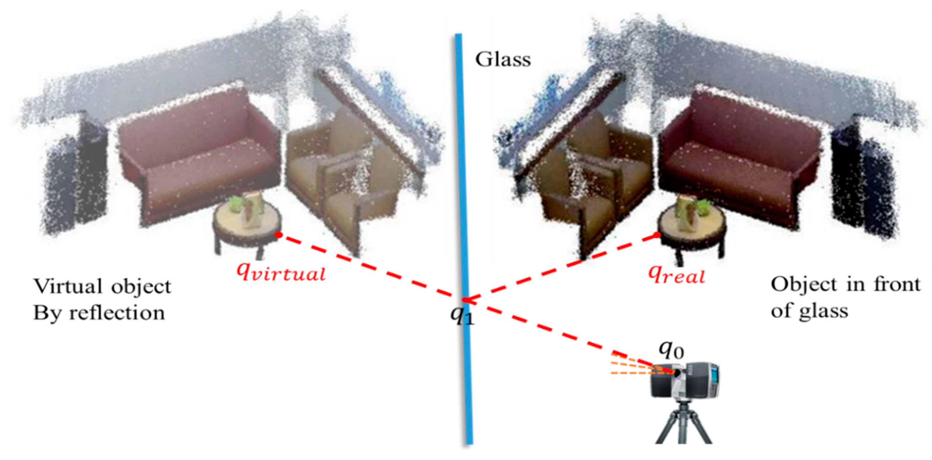
Light is reflected by objects, such as glass, which forms undesired objects of the reflected scenes. When capturing large-scale 3-D point clouds using LiDAR sensors, laser pulses emitted from the scanner also result in the formation of undesired reflection artifacts and virtual points in the 3-D space. Figure 1 shows an example of a reflection caused by the LiDAR sensor. The LiDAR sensor measures the distance from the scanner to the target object by emitting laser pulses and receiving their return pulses based on the propagation time of light. In this case, the laser is reflected to other objects because of the reflective nature of the glass when the sensor emits the laser light onto the glass.
Consequently, the distance detected by the scanner is actually the sum of the distance from the scanner to the glass and the distance from the glass to the object in front of the glass . As the scanner is unaware of the presence of the glass, the received pulse is considered the direct reflected pulse of the straight line that reaches the scanned object. Therefore, the scanner produces a virtual object in the plotted point cloud data.
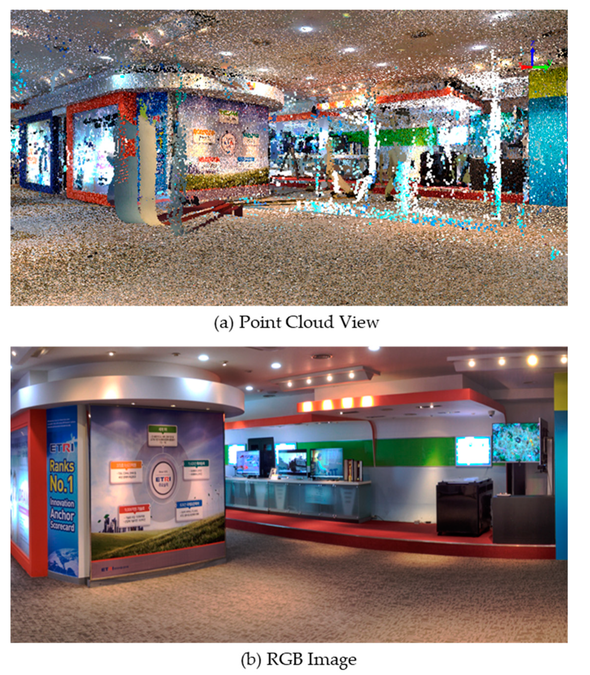
This virtual object produced by the reflective area reduces the quality of the point cloud. This problem worsens when the sensing area has many windows or glass materials, which are a typical part of the design in modern buildings. As shown in Figure 2, there are many reflective materials in a large area; thus, the scale of the noise generated in the reflective area is also large. Traditional noise filtering methods used for point clouds, such as the statistical outlier removal method, cannot remove dense noise. Therefore, noise produced by the reflective area cannot generally be filtered. This study proposes a dense reflective noise filtering method for large-scale point clouds using the multi-position LiDAR sensing data.
The proposed method removes the dense reflective noise by calculating the depth reflection intensity variance within a certain area and by comparing it with the position sensing data. The proposed method is applicable to large-scale point clouds with high indoor density and can effectively filter dense noise.
The contributions of this study are summarized as follows:
- To the best of our knowledge, this study is the first to implement the noise region denoising for large-scale point clouds containing only single-echo reflection values.
- Most current methods are based on statistical principles to remove some of the noise. However, these conventional methods cannot differentiate the reflected noise from other normal objects. The method proposed herein successfully solves this problem.
- The proposed method can be applied to large-scale point clouds. The methods used in previous studies were only for the point clouds of individual objects or for areas with sparse point cloud density. The proposed method can denoise large-scale point clouds using multiple sensing data.
Therefore, this study successfully performs the denoising of dense and large-scale point cloud data collected from several positions and multiple scenes. Additionally, this study conducted a comparison experiment using FARO SCENE [10] as a benchmark. The experimental results clearly indicate that the proposed method successfully eliminates most of the noise due to reflections when compared with the denoising method of FARO SCENE. The successful removal of reflection noise significantly contributes to further usage of point clouds in techniques, such as 3-D reconstruction, and has a considerable impact on applications, such as point cloud reconstruction.
2. Related Work
Reflection removal, which involves the removal of interference due to the reflections from glass surfaces, is a technique of great interest in computer vision. Several studies [11,12,13,14] have attempted to remove reflections from single glass images in the field of image processing and achieve reflection removal by simultaneously using multiple glass images. Conversely, LiDAR uses active light irradiation technology, emitting laser pulses and calculating their return time, to measure distance. The noise generated by reflecting objects has a greater impact on LiDAR production.
From [15], point cloud denoising techniques are classified into seven categories: statistical-based filtering techniques, neighborhood-based filtering techniques, projection-based filtering approaches, signal processing-based methods, PDEs-based filtering techniques, hybrid filtering techniques, and other methods. These methods can effectively remove the outliers from point clouds in specific cases, such as the point cloud models with added Gaussian noise. However, they are not effective in the removal of the reflection noise.
In recent years, various methods have been developed using clustering algorithms to detect point cloud noise [16,17,18,19,20,21,22,23,24,25,26]. Li et al. [27] proposed an improved K-algorithm for color-based clustering of point clouds to detect outlier points. Czerniawski et al. [28] proposed a point cloud outlier detection method based on density clustering. Rusu et al. [29] and Weyrich et al. [30] proposed local density-based outlier detection methods to determine whether a point is an outlier or not, based on the number of domain points. However, in large-scale point clouds, the number of noise region points is also particularly large, and the clustering algorithm cannot efficiently detect the reflection noise.
The traditional point cloud denoising methods focus on removing the outliers in the point cloud data, which generally contain only the coordinate data. The reflected intensity is the intensity of the returned laser beam obtained by the LiDAR after the emitted laser beam reaches the specified object. The value of the reflection intensity is generally related to the material of the object and its optical properties. The reflectivity and optical properties of different materials vary [31,32,33,34]. Standard materials, such as wood, walls, or clothes, generally provide diffuse reflection of laser light, which is suitable for LiDAR sensors as there is no absorption or specular reflection. Conversely, reflective surfaces, such as mirrors or glass, reflect incident laser light. A glass surface primarily exhibits specular reflection and transmittance for a slight diffuse reflection of laser light [35,36,37,38]. The reflected noise can be detected with the help of these optical properties. This process has been summarized in previous studies in four ways. First, Koch et al. [39,40] detected the reflective area based on the properties of the material; various materials have different properties under laser irradiation, including reflection, scattering, or absorption. Second, Wang et al. [41,42] and Ali et al. [43] detected the reflective region by mirror symmetry because the reflective noise follows the reflection rule of light, and the reflective area can be detected by the distribution of the pairs of points. Velten et al. [44] detected the noise areas through the phenomena commonly observed in the reflective areas, such as glass windows, which generally produce noise with an empty square in the center. Finally, Mei et al. [45] detected reflected noise with the help of special sensor data, such as multi-echo LiDAR and the reflected intensity values.
These methods effectively improve the accuracy of the detection of the reflected noise in SLAM. However, the point cloud data used in SLAM are sparse. Therefore, these methods are not suitable for large-scale point clouds. Yun et al. [46,47] proposed a method to remove the virtual points formed due to glass planes in a large-scale point cloud. However, this method employs multiple echoes of the LiDAR data and is not applicable to large-scale point clouds that do not contain the multi-echo data.
3. Proposed Method
3.1. Overview
This study uses the point cloud data obtained from the LiDAR sensor to detect noise due to highly reflective objects by integrating the LiDAR point cloud data obtained from multiple locations together and then to remove noise to reconstitute the noise-free 3-D point cloud data. Figure 3 shows an overview of the entire point cloud denoising system.
The point cloud data in this study contain the scan location information (i.e., location of the LiDAR sensor, point location information, XYZ, color information, RGB, and reflection value information). Typically, the scanned data contain several individual scan files, each of which is obtained from one scan. Multiple scans are performed at different locations in a region, and the point cloud of this region is obtained after merging. To eliminate the large amount of noise in the merged point cloud files, the method proposed in this paper processes each scan file in a certain order. The proposed method is divided into three modules. The first module is the data pre-processing module, which converts the 3-D point cloud data into a 2-D distance image format. The second module is the reflective area detection module, which detects the presence of a reflective area by calculating the variance value in each window using a sliding window. The third module is the noise removal module, which compares the reflective areas with the sensor data from the other locations to obtain the exact noise locations. This module also includes a location selection module to improve the accuracy of the noise detection by optimizing the selection of the other sensor locations.
3.2. Data Preprocessing Module
This module is designed to convert the 3-D point cloud data into 2-D range images. In this study, the coordinate data obtained from the point cloud data were converted to depth range images, and the reflection intensity values in the point cloud data were converted to reflection range images.
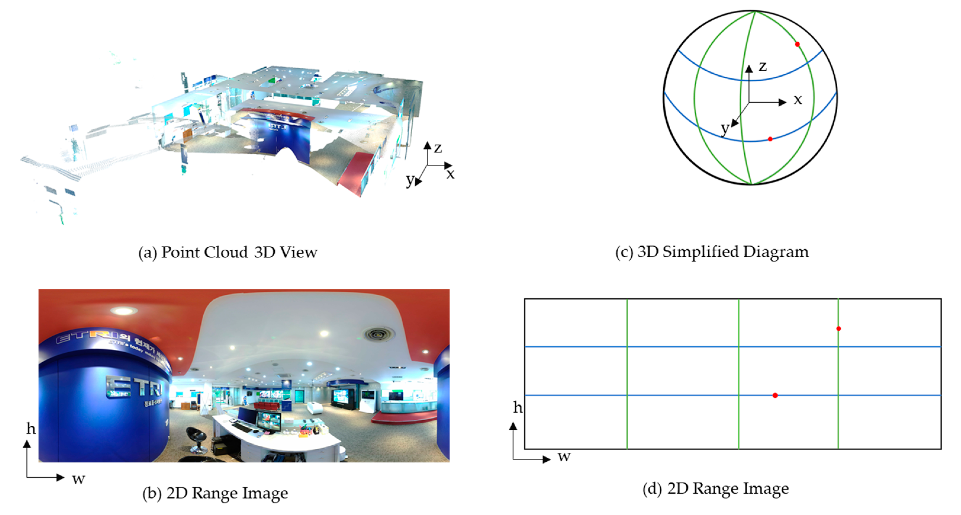
The LiDAR points are clearly ordered along the scanlines, forming the first dimension of the sensor topology, linking each LiDAR pulse to the immediately preceding and succeeding pulses within the same scan line; the topology of the sensor also varies with the LiDAR sensor model being used. Three-dimensional LiDAR sensors involve multiple simultaneous scanline acquisitions. Each scanline contains the same number of points, and each scanline may be stacked horizontally to form the same type of structure. Therefore, any measurement of the sensor may be arranged in a H × W image [48], where H (height), W (width) refers to the two-bit matrix with H, W as the coordinate system, H, W depends on the setting of the Lidar sensor. It is related to the scanning angle range and resolutions. With the stereographic projection method, we can project the XYZ coordinate system of the 3-D point cloud into the 2-D plane, as shown in Figure 4. The principle is similar to that of panorama, where the point cloud of a scene is simplified to a sphere, as shown in Figure 4c, where each red point represents a point in the point cloud and each point contains information on the position, color, and reflection values. Figure 4b shows the range image, which only shows the color information of each point. The figure also shows how the sensor topology stretches the 2-D image. The point cloud is defined as a matrix of N × (3 + D), where N is the number of points contained in the point cloud, 3 is the coordinates of the point cloud, and D is other information of the point cloud (e.g., color and reflection value). The range image can be defined as a matrix of H × W, where H and W are determined by the size of the point cloud. In this study, such images are only constructed as the pixel reflection intensity using the range calculation, later referred to as range images. When the pulses emitted by the LiDAR sensors are absorbed by the target object due to the reflecting surfaces, or in the absence of a target object (e.g., the sky), the laser is generally unable to measure the distance. Consequently, during the generation of range images, there are a large number of missing points owing to the absence of measurements. In this study, 0 is used to replace missing parts. Additionally, the data used in this study only contain the intensity values of a single laser return. The data for which multiple laser return values are acceptable are beyond the scope of this study.
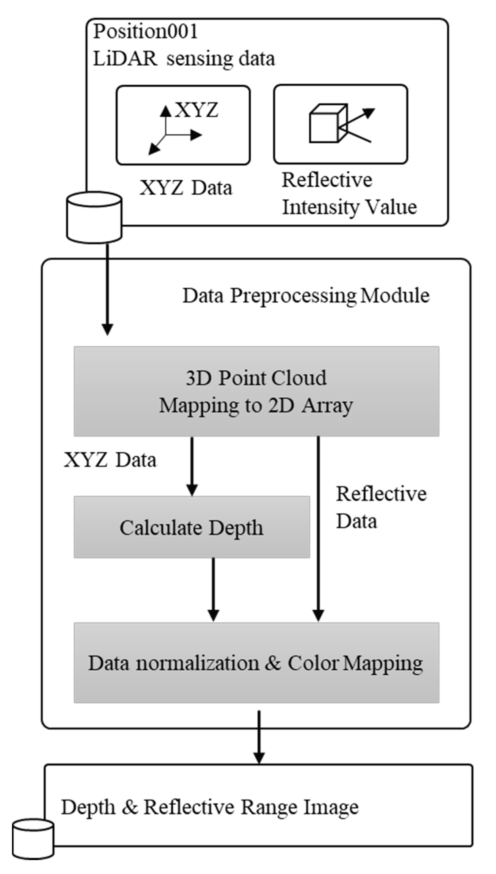
Figure 5 shows the data preprocessing steps that convert the point cloud data to range images. The LiDAR scanned data are first converted into a 2-D matrix, and the point cloud coordinate data are mapped to the color code after calculating the depth value to generate the depth range image; the reflection value data are then directly mapped to the code to generate the reflection range image.
The method of extraction of range images is as follows. The distance between each point and the sensor is calculated for each point pi in the point cloud , which is called the depth in this study, considering the sensor position as the origin. First, the x, y, and z values are mapped to the 2-D image format by topology. The depth values are then calculated using the formula shown in Equation (1) to determine the distance:
where is the LiDAR sensor position, and is the position of each point in the point cloud .
After normalizing the original data, a grayscale map can be generated. Since the nuances of the grayscale map are not suitable for observation. This study uses the ‘cv::applyColorMap’ function provided by OpenCV [49] to transform grayscale maps. Thus, a color range image was obtained. The color mapping is performed only to facilitate the observation of the features. Only the raw data were used in this study for data processing, and no color mapping was performed. Figure 5 schematically illustrates the process of converting the range image. Examples of reflectance range images and depth range images are shown in Figure 6.
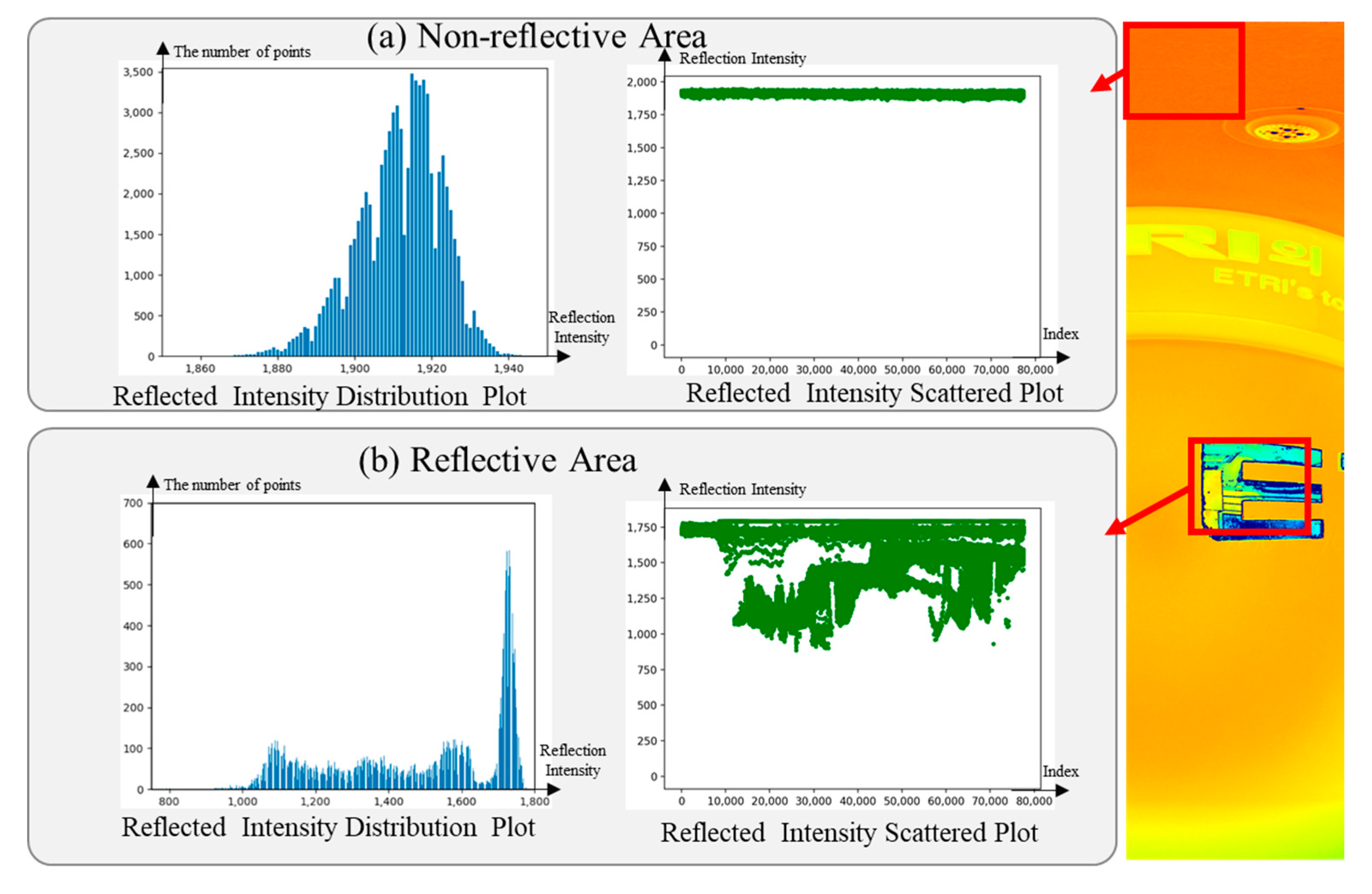
The reflection area is analyzed using the reflection intensity and the depth range images, as shown in Figure 7. The reflection range image is used as an example to show the characteristics of the noise point regions. The Shapiro–Wilk test [50] is used to test whether the data conform to a Gaussian distribution. The W statistic is calculated as follows:
where is the order statistic, and is the sample mean. The coefficients and are the expected values of the order statistics of independent and identically distributed random variables sampled from the standard normal distribution and is the covariance matrix of those order statistics. In the initial experimental analysis, this paper uses Equation (2) as a condition to determine the noise area by whether it conforms to the Gaussian distribution.
Figure 7 shows the reflection range image obtained by the reflection value mapping. The reflection values are plotted within a certain region in a scatter plot and a distribution plot, where the horizontal coordinate of the distribution plot is the reflected intensity value of the selected area and the vertical coordinate is the number of a certain value. The scatter plot has the index of the points in the horizontal coordinate and the reflection intensity value of each point in the vertical coordinate. Note that in Figure 7, the coordinate system ranges of the reflection intensity distribution plot are not consistent. In the non-reflective region selected in Figure 7a, the reflection intensity is concentrated between 1854 and 1945 with a W-statistic value of 0.981, while in the reflective region selected in Figure 7b, the reflection intensity is divided between 885 and 1792 with a W-statistic value of 0.823. When the laser emitted by LiDAR shines on the same object, the intensity of the echo reflection received by LiDAR is similar. Additionally, when the laser shines on a highly reflective object, it is reflected to other objects due to reflection. Thus, the distribution of the reflection intensity obtained is chaotic. The features are grouped into two categories based on extensive experimentation. The first category is the general area, as shown in Figure 7a, which does not contain noise and is composed of the same material; the distribution of the reflection values in this area is normal and the scatter plot shows that this part of the distribution is relatively uniform. The second category is the noise region, as shown in Figure 7b, which contains the reflective substances, which are smooth metallic materials in this case. The light emitted from the LiDAR is reflected at different locations due to the presence of the reflective substances. Therefore, the reflection values in this part are generally cluttered, as shown in the scatter and distribution diagrams in part b. The reflection values are quite complex, and the range is quite large to be shown in the distribution diagram. The reflected intensity values in the normal region are normally distributed, whereas the reflected intensity values in the reflective region are irregular. Thus, the normal area can be distinguished from the reflective area using this feature.
3.3. Reflective Area Detection Module
We also define a set that takes from every sliding window using the sliding value . Then, we define a set as:
where is the depth variance threshold and is the reflection variance threshold.
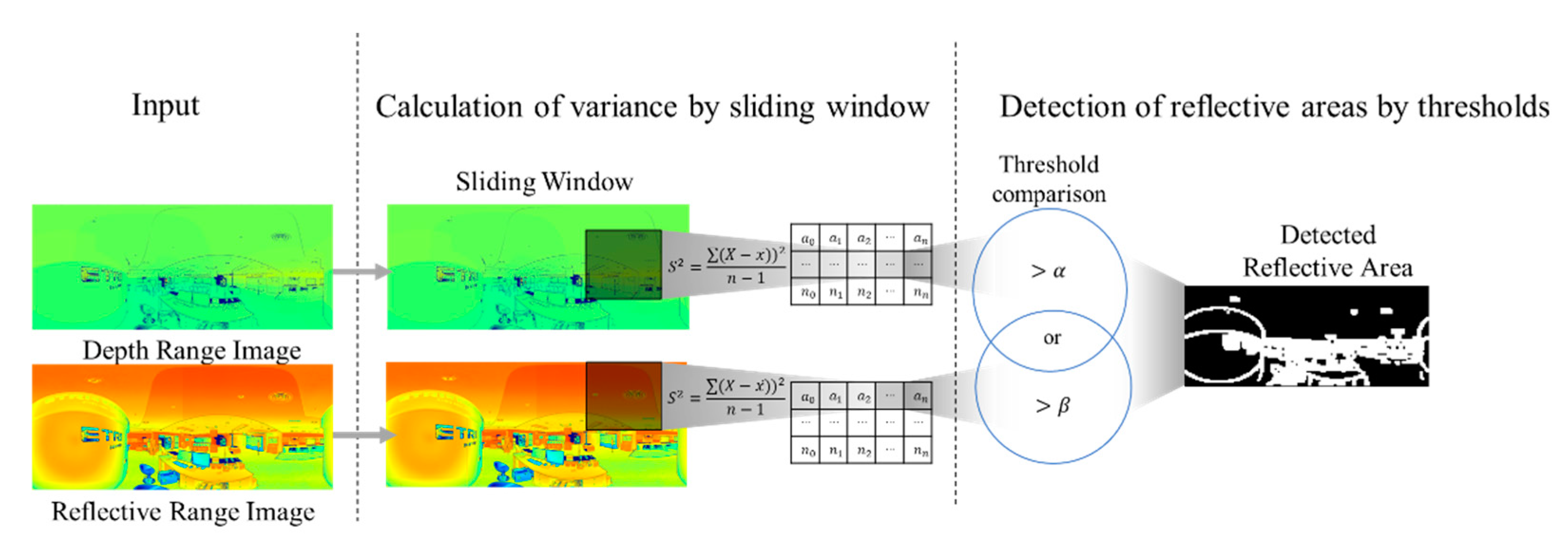
The process of the reflective area detection module is as follows. First, we create an window with i as a step and slide the image in the depth and the reflection intensity range. The depth variance array and reflection intensity variance array is obtained by calculating the variance of the window (Equation (4)). The variance is a measure of the dispersion of a set of data, where the mean of the squared differences between each sample value and the mean of the overall sample value is used. Taking the data of the selected region in Figure 7 as an example, for the non-reflective region, the W statistic value is 0.981 and the variance is 118.456, and for the reflective region, the W statistic value is 0.823 and the variance is 59,776.815. Since the range of the W statistic value is in 0–1, and the variance of the response to the characteristics of the data distribution, the larger the variance, the higher the data dispersion. So, this paper selects the data with high dispersion as the candidate area of noise region by calculating the variance of the data in the selected area. Therefore, the noise area can be effectively detected by comparing the variance of the reflection intensity and the distance. The depth variance array and the reflection intensity variance array are filtered by setting a threshold value that is greater than the set value and is considered to contain noise in this window. The depth variance array and the reflection intensity variance array are concatenated to obtain the final 2-D array containing the noisy region:
where is the average value.
This section presents the method to detect the region where the reflection noise exists. The method calculates the variance based on a sliding window through the distribution characteristics of the reflection noise. As shown in Figure 8, the variance value of the selected window is calculated by setting a sliding window of on the depth and the reflective range image, in the data preprocessing step. If the depth variance or the reflection intensity variance within the selected window is greater than the set threshold α and β (here, α is the depth variance threshold, and β is the reflection variance threshold), this window is regarded as the window containing noise. All the data are then detected through the sliding window. Let us define a set of points , where is the variance calculated from the set of points selected by the sliding window .
3.4. Noise Removal Module
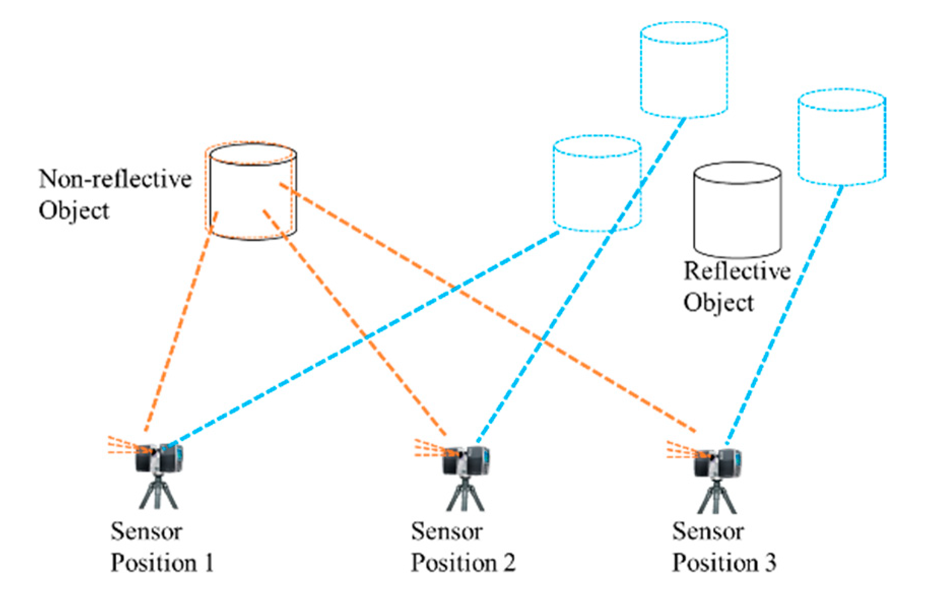
As the reflective area noise is related to the position and the angle of the sensor, the noise generated in the reflective area is different for the sensors in the various positions, as shown in Figure 9. When the LiDAR sensors located at different locations irradiate an object, the point cloud data of the object are obtained. After registering and merging the point cloud data of all the position sensors, they are represented as global coordinates. Consequently, if it is ordinary data, the coordinate points of its point cloud are all identical. However, if it is a reflective object, the sensors located at different positions produce different artifacts because of the nature of the reflection.
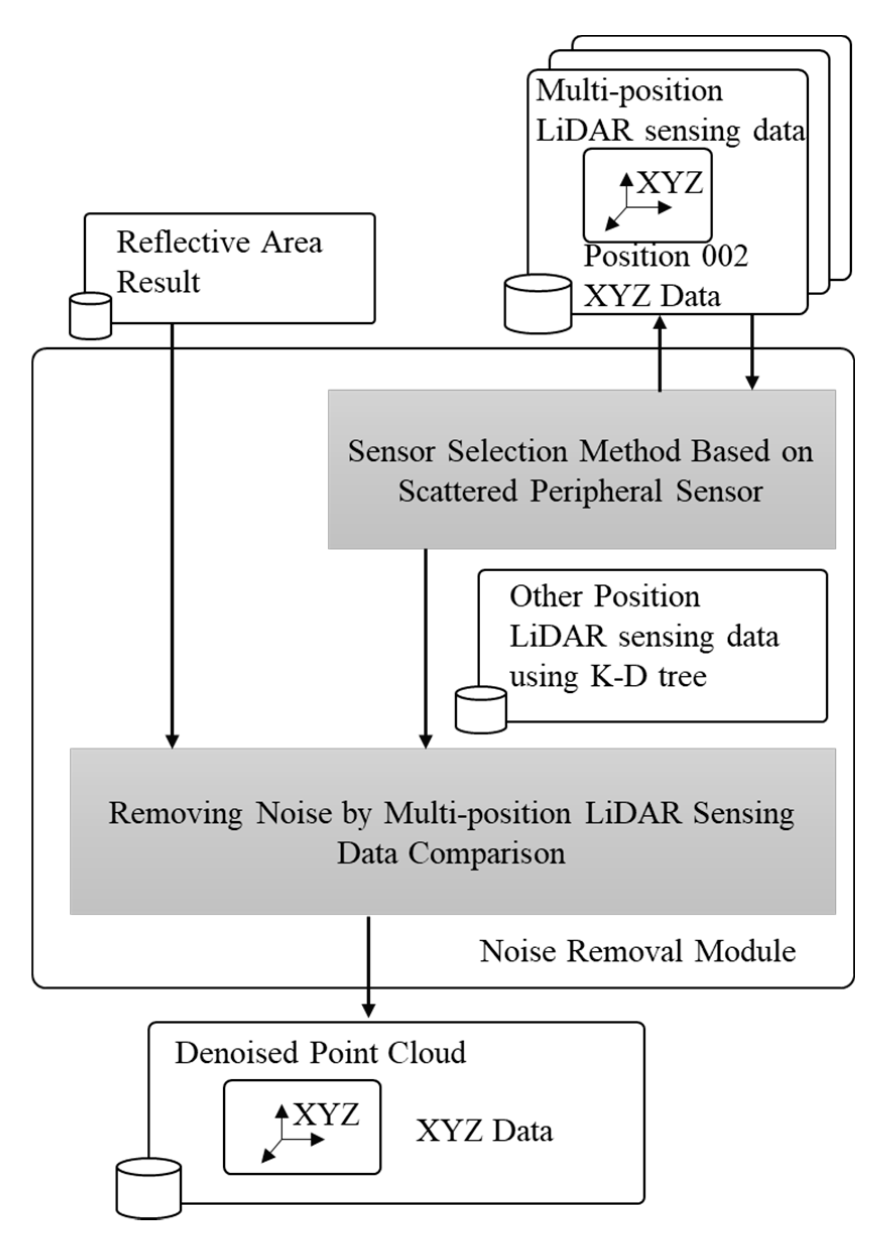
The noise removal module contains two parts, as shown in Figure 10: the selection method based on the scattered peripheral sensors and the removal of noise by the multi-position LiDAR sensing data comparison.
We input four thresholds in this module: the threshold of deleting the nearest sensor γ, matching point threshold δ, number of the nearest sensor ε, and radius of the distance ζ. First, the target sensor reflection area results are loaded sequentially; the LiDAR sensor position data are loaded and sorted based on the distance to the target sensor position. After deleting several sensors closest to the target sensor based on the threshold value γ, the point cloud data from the remaining sensors are loaded into the k-d tree according to the threshold value ε. Based on the noise part of the reflective area result of the target sensor, the coordinate value of the noise point is obtained from the original point cloud data by the index of the noise point, and the coordinate value of the noise point is used to search in the k-d tree. If other points can be searched within the threshold ζ, and the number of points searched is greater than the threshold δ, the point is a normal point; otherwise, it is a noise point. Finally, the coordinates of the normal points are obtained from the original point cloud by using the index of all the normal points and are saved as the denoised point cloud. The main algorithm that processes multiple sensing data is Algorithm 1.
| Algorithm 1. Noise removal using multi-position LiDAR sensing data comparison |
| Input: Threshold_of_deletes_nearest_sensor γ, Matching_point_threshold δ, Number_nearest_sensor ε Radius_distance ζ Peripheral LiDAR sensor position list Target LiDAR sensor position () |
| Output: DenoisePointCloud |
| For target sensor reflective area result from target sensor position () Load Peripheral LiDAR position data from LiDAR sensor position Sort Peripheral LiDAR position data from LiDAR sensor position Delete peripheral sensors position around the target sensor () by threshold γ. Select peripheral sensors by threshold ε. Load peripheral sensors point cloud from peripheral sensors position into k-d tree for each noise point do find original location from point cloud search noise point from k-d tree if presence of other points in threshold ζ & number of points searched > δ then add to normal point else add to noise point end for for normal point Search point cloud location using normal point index Save denoise point cloud end for end for |
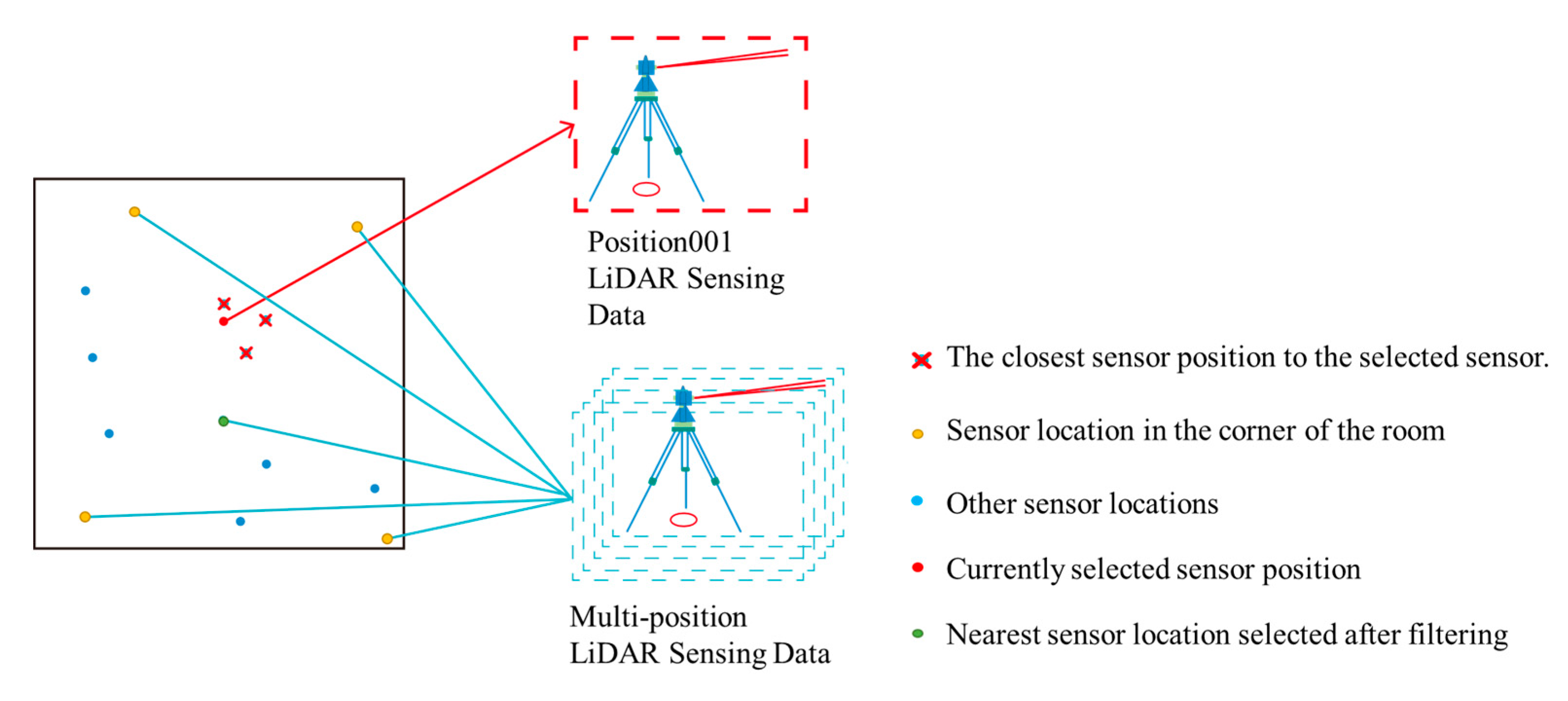
Through extensive experiments, this study concluded that sensors located in the corners of the room generate less noise and can effectively capture the structure of the room. Therefore, the four sensor locations in the corners of the room are always reserved for data comparison. As the data obtained from the closer sensors are similar to the selected sensor noise positions, we need to remove several sensor data from the closest positions of the selected sensor. The details are shown in Figure 11. After removing the closest sensors to the selected sensor, we select the current closest sensors and four sensors in the corners of the room for data comparison. This diagram is a simplified version of the scattered peripheral sensor selection method and the actual application. The specific parameters vary depending on the scenario, owing to the large number of sensor locations and the complexity of the situation.
4. Experiments and Evaluation
4.1. Data Acquisition
The data used in this study were obtained from FARO Focus 3D X 130 [51]. We used this device to capture real indoor scenes. The main data came from the ETRI exhibition hall. The area is about , which contains a large number of displays and glass areas. Other data came from indoor locations, such as conference rooms (about ) and museums (about ). Most of the scanner settings use default settings. Some of the settings data are provided in Table 1, which may be changed for different scenarios. Here, we only provide the more typical scanner settings data. Point cloud registration is courtesy of FARO SCENE [10].
4.2. Generation of Ground Truth Data and Experimental Environment
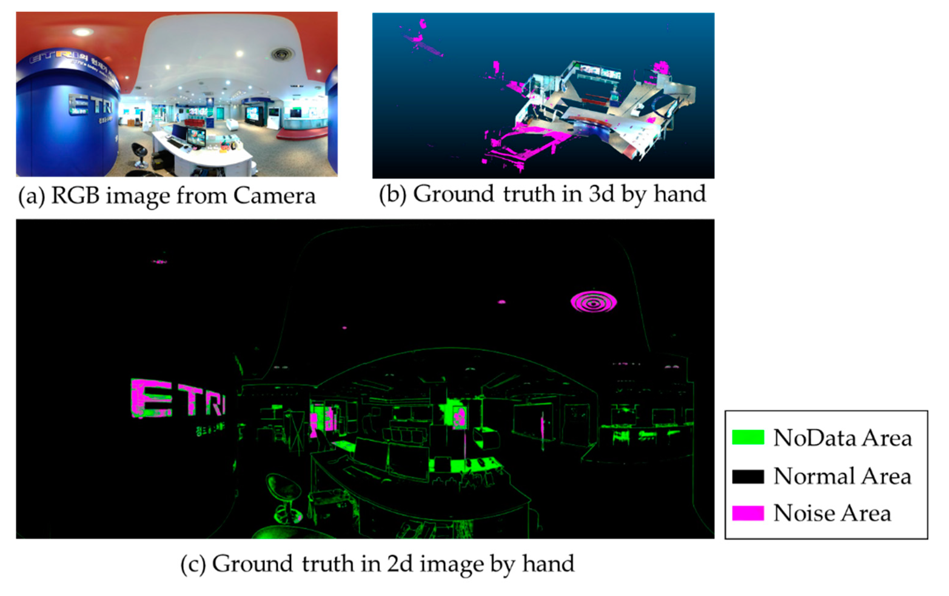
As current data do not contain the ground truth (GT) data, 15 scenes are manually denoised, and the GT data are generated to test the effectiveness of the proposed method. In Figure 12, (a) shows the RGB image of the same scene, (b) shows the point cloud image of the same scene, and (c) is the manually labeled GT image, where the green part is the no-data region. The lasers do not provide the measured distances due to the reflective surfaces, absorption by the target object, or due to non-existence. Black is the normal region, and purple is the noise region.
Experiments were conducted using a desktop computer, with the following specifications: Windows 10 operating system and an Nvidia RTX 2080Ti GPU. An Intel Core i9-9900 CPU running Python 3.8 is configured to the system. FARO SCENE [10] software is used to denoise the point clouds to compare the effectiveness of the methods proposed in this paper. FARO SCENE [10] is a comprehensive 3-D point cloud processing and management software tool. It also contains the common tools used for point cloud registration and processing. In this experiment, three point cloud noise filters were used, which include a dark scan point filter, a distance filter, and a stray point filter. The dark scan point filter removes all scan points whose reflection value is below a given threshold. The distance filter is used to remove scanned points within a specified range from the laser scanner data. The stray point filter has the same application field as the outlier filter. The specific parameters are listed in Table 2.
The point cloud data used in this study are quite dense, and the number of points and the noise points in the point cloud in each scene are listed in Table 3. The data obtained varies slightly from the set resolution due to the sensor and the place where the data are collected.
4.3. Noise Detection and Performance
This study uses the same evaluation criteria as in [52] to quantitatively analyze the proposed method. Noise is referred to as an outlier in this section for comparison purposes. The outlier detection rate (ODR) is used to calculate the detection performance. The noise detection rate is the ratio of the number of noises correctly identified by the proposed method to the total number of noises, as expressed in Equation (5): the higher the ODR, the greater the noise detected by the proposed method. The inlier detection rate (IDR) is the ratio of the number of inliers correctly identified by the proposed method, to the total number of inliers, as expressed in Equation (6): the higher the IDR, the greater the number of inliers detected by the proposed method. The false positive rate (FPR) is the ratio of the inliers identified as outliers to the total number of inliers: the lower the FPR, the lower the rate at which the proposed method identifies outliers as inliers. The false negative rate (FNR) is the ratio of outliers identified as inliers to the total number of outliers: the lower the FNR, the lower the rate at which the proposed method identifies inliers as outliers. Accuracy refers to the ratio of the correct predictions (correct outlier and correct inlier) across all the points. If all the points are marked as outliers, the ODR becomes one. Similarly, if all the points are marked as inliers, the IDR becomes one. When the above four ratios are combined, the accuracy rate illustrates the effectiveness of the proposed method in detecting the outliers. The ODR, IDR, FPR, FNR, and the accuracy are defined as follows:
where TP and TN indicate the number of outliers and inliers that are correctly defined, respectively.
Table 4 compares the results obtained in this study with the results obtained from the FARO filter. The results obtained by the proposed method are superior to those of the FARO filter regarding the ODR, IDR, FPR, and FNR. This demonstrates that the proposed method can effectively detect the outliers and the common points and the FPR and the FNR are significantly lower than those of the FARO filter. Note that the objective it is to obtain higher values of ODR and IDR and the lower values of FPR and FNR.
Table 5 shows the accuracy of the results of the proposed method, compared to that of the FARO results. As expressed in Equation (9), the accuracy value is the ratio of the accurately detected outlier and inlier points, to all the points. As the density and the scale of the point cloud data used in this study are exceptionally large, and the inlier points account for the vast majority. The results of the proposed method are only slightly better than those of FARO in the comparison of the accuracy values. However, the images presented in the paper evidently show that the proposed method successfully removes most of the outliers that are due to reflections.
4.4. Noise Detection and Performance
In this section, we present the results obtained by the proposed method in the form of pictures.
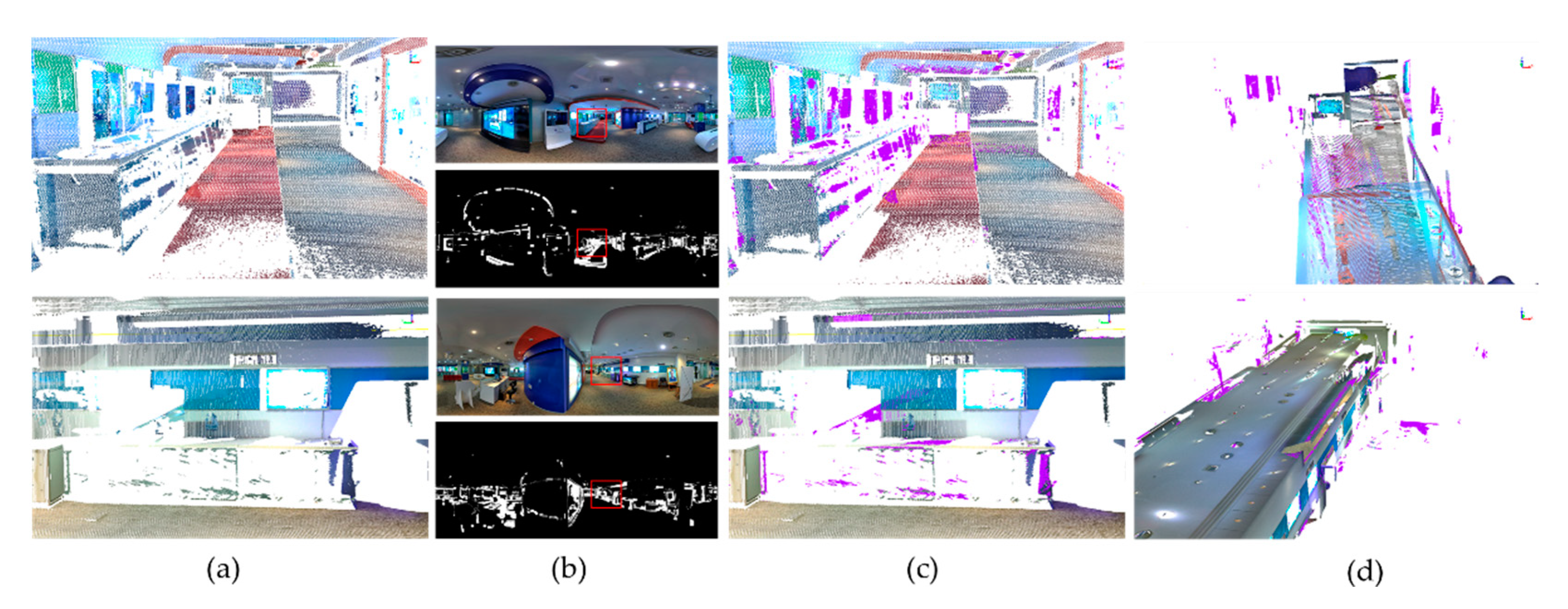
In Figure 13, the point cloud reflection noise detection results of some sensors are shown. Here, (a) is the original point cloud, and (b) is the RGB image and the 2-D results obtained by the proposed method, respectively, and the white area is the detected noise area, which can be observed in the RGB image. Further, (c) and (d) show the noise detection results from different angles. The purple part shows the noise detected by the proposed method.
Figure 14 shows our results compared to the point cloud after manual denoising. This image contains scanned data from 15 scenes. Here, (a) is the original point cloud, (b) is the point cloud detected by our method, (c) is the point cloud after denoising using our method, and (d) is the point cloud after manual denoising.
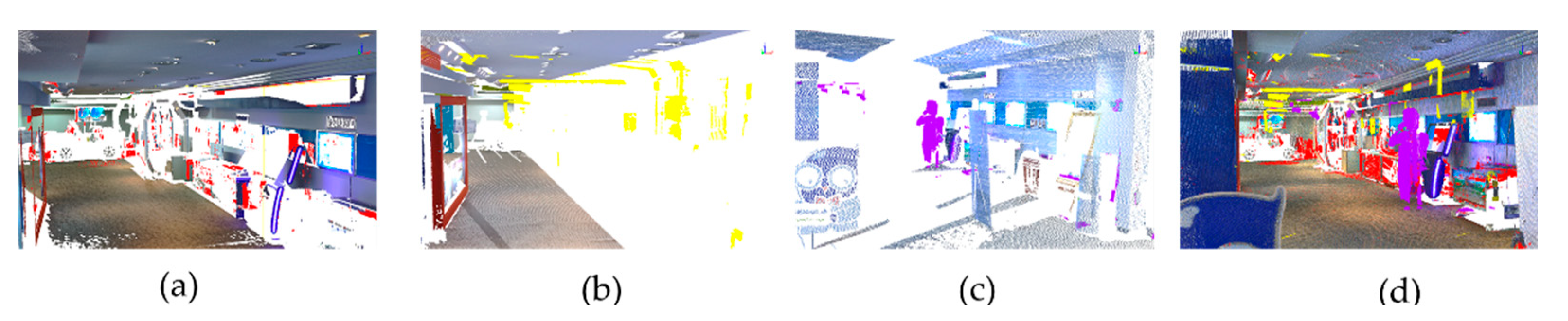
In Figure 15, we show the data after merging all sensors and the data from a single sensor. In part (a)(b)(c), separate sensor data from three different locations are shown with red, yellow, and purple areas of reflected noise, respectively. The result of combining sensor data from multiple locations is shown in (d).
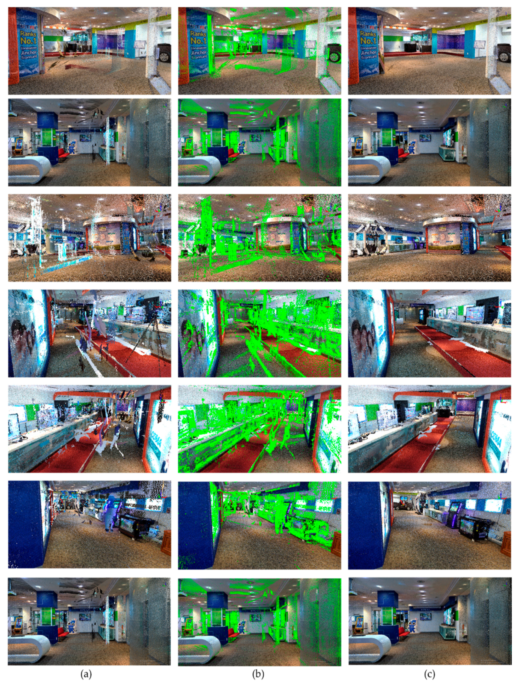
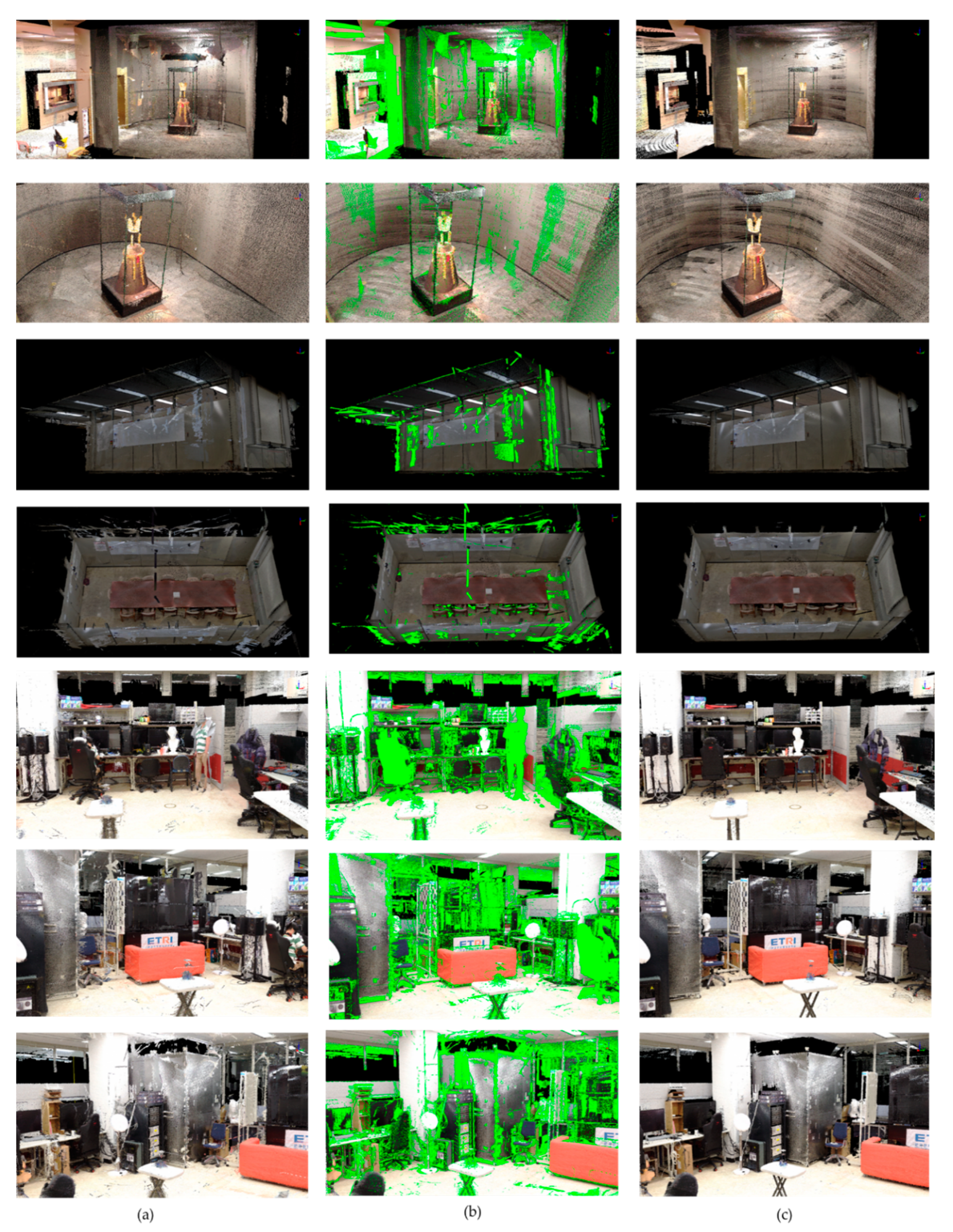
Figure 16 illustrates the results of the proposed method. The green part of the figure shows the noise area. This image contains scanned data for a total of 72 scenes.
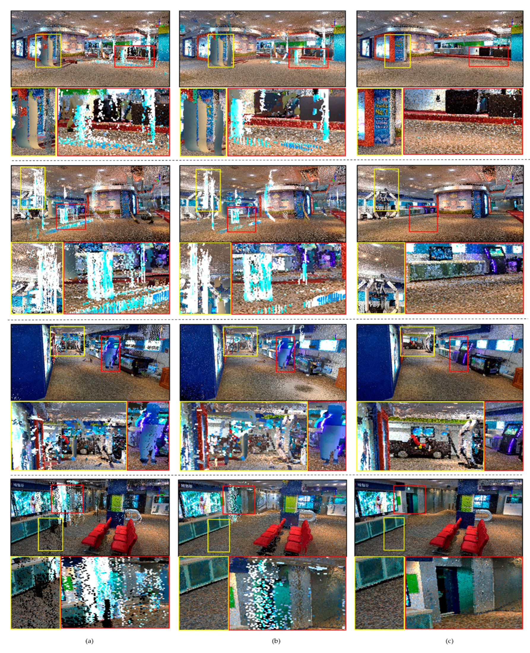
Figure 17 shows a comparison of the proposed results with the FARO SCENE denoising results. Here, (a) shows the original point cloud view, (b) shows the result after the FARO SCENE denoising, and (c) shows the denoising result obtained from the proposed method. The images evidently show that most of the noise due to reflections can be effectively removed using the proposed method. Additionally, noise generated by moving objects can be effectively removed. This image contains scanned data for a total of 72 scenes.
Figure 18 shows the results when the proposed method is applied to other datasets (other buildings in different areas) to verify the generalized performance of the algorithm. In the other datasets, the proposed method is observed to effectively remove the noise generated by reflections and the noises generated by moving objects.
5. Discussion and Conclusions
This paper proposed a method to remove reflection noise in high-density point clouds. In this method, the 3-D point cloud data were first converted into 2-D range image data, and the reflected noise area was detected by calculating the variance in the range image. The detected noise area was then compared with the point cloud data from sensors at other locations to determine the specific noise location and to remove the noise. Experiments show that this method is more effective in removing dense large-scale noise caused by reflections and moving objects when compared to the traditional methods. In this study, the point cloud data collected from several different buildings were tested, and good results were obtained, indicating that the proposed method has wide applicability and can effectively remove large reflective noise regions from dense point clouds. Therefore, this study effectively fills the gap in handling large-scale point clouds by the traditional methods. To the best of our knowledge, this study is the first to implement noise region denoising for large-scale point clouds containing only single-echo reflection values. This paper also uses FARO SCENE as a benchmark for comparison experiments, and the proposed method in this paper is significantly better than other denoising methods. Consequently, a good result was achieved.
In the current work, the reflection intensity value data were used for initial noise area detection. Further, the location information of each point was used to detect the final noise location via comparison with the point locations from other location sensors. However, a drawback is that an accurate noise region must be obtained by comparing the point cloud positions with those obtained from sensors at other locations. In future work, we will use a machine learning approach to detect noise regions using only sensor data from a single location.
Author Contributions
Conceptualization, R.G.; Data curation, X.H.; Funding acquisition, K.C.; Methodology, R.G. and J.P.; Project administration, K.C.; Supervision, K.C.; Writing—original draft, R.G.; Writing—review and editing, J.P., X.H., S.Y., and K.C. All authors have read and agreed to the published version of the manuscript.
Funding
This research was funded by Electronics and Telecommunications Research Institute (ETRI) grant funded by the Korean government. [20ZH1200, The research of the fundamental media·contents technologies for hyper-realistic media space] and the Dongguk University Research Fund of 2020 (S-2020-G0001-00050).
Institutional Review Board Statement
Not applicable.
Informed Consent Statement
Not applicable.
Data Availability Statement
The data presented in this study are available on request from the corresponding author. The data are not publicly available due to that the information of cultural relics and the research facilities is involved, that cannot be opened without authorization.
Conflicts of Interest
The authors declare no conflict of interest.
References
- Mehendale, N.; Neoge, S. Review on Lidar Technology. Available online: https://ssrn.com/abstract=3604309 (accessed on 2 August 2021).
- Vines, P.; Kuzmenko, K.; Kirdoda, J.; Dumas, D.C.S.; Mirza, M.M.; Millar, R.; Paul, D.J.; Buller, G.S. High performance planar germanium-on-silicon single-photon avalanche diode detectors. Nat. Commun. 2019, 10, 1–9. [Google Scholar] [CrossRef] [Green Version]
- Huang, Z.; Lv, C.; Xing, Y.; Wu, J. Multi-modal Sensor Fusion-Based Deep Neural Network for End-to-end Autonomous Driving with Scene Understanding. IEEE Sens. J. 2020, 21, 11781–11790. [Google Scholar]
- Tachella, J.; Altmann, Y.; Mellado, N.; McCarthy, A.; Tobin, R.; Buller, G.S.; Tourneret, J.Y.; McLaughlin, S. Real-time 3D reconstruction from single-photon lidar data using plug-and-play point cloud denoisers. Nat. Commun. 2019, 10, 1–6. [Google Scholar] [CrossRef] [Green Version]
- Tachella, J.; Altmann, Y.; Ren, X.; McCarthy, A.; Buller, G.S.; McLaughlin, S.; Tourneret, J.-Y. Bayesian 3D Reconstruction of Complex Scenes from Single-Photon Lidar Data. SIAM J. Imaging Sci. 2019, 12, 521–550. [Google Scholar] [CrossRef] [Green Version]
- Kuzmenko, K.; Vines, P.; Halimi, A.; Collins, R.; Maccarone, A.; McCarthy, A.; Greener, Z.M.; Kirdoda, J.; Dumas, D.C.S.; Llin, L.F.; et al. 3D LIDAR imaging using Ge-on-Si single–photon avalanche diode detectors. Opt. Express 2020, 28, 1330–1344. [Google Scholar] [CrossRef]
- Schwarz, B. Mapping the world in 3D. Nat. Photonics 2010, 4, 429–430. [Google Scholar] [CrossRef]
- Huo, L.-Z.; Silva, C.A.; Klauberg, C.; Mohan, M.; Zhao, L.-J.; Tang, P.; Hudak, A.T. Supervised spatial classification of multispectral LiDAR data in urban areas. PLoS ONE 2018, 13, e0206185. [Google Scholar] [CrossRef]
- Altmann, Y.; Wallace, A.; McLaughlin, S.; McLaughlin, S. Spectral Unmixing of Multispectral Lidar Signals. IEEE Trans. Signal Process. 2015, 63, 5525–5534. [Google Scholar] [CrossRef] [Green Version]
- FARO SCENE. Available online: https://www.faro.com/en/Products/Software/SCENE-Software (accessed on 2 August 2021).
- Levin, A.; Weiss, Y. User assisted separation of reflections from a single image using a sparsity prior. IEEE Trans. Pattern Anal. Mach. Intell. 2007, 29, 1647–1654. [Google Scholar] [CrossRef] [PubMed]
- Fan, Q.; Yang, J.; Hua, G.; Chen, B.; Wipf, D. A generic deep architecture for single image reflection removal and image smoothing. In Proceedings of the IEEE International Conference on Computer Vision, Venice, Italy, 22–29 October 2017; pp. 3238–3247. [Google Scholar]
- Wan, R.; Shi, B.; Duan, L.Y.; Tan, A.H. Crrn: Multi-scale guided concurrent reflection removal network. In Proceedings of the IEEE Conference on Computer Vision and Pattern Recognition, Salt Lake City, UT, USA, 19–21 June 2018; pp. 4777–4785. [Google Scholar]
- Zhang, X.; Ng, R.; Chen, Q. Single image reflection separation with perceptual losses. In Proceedings of the IEEE conference on computer vision and pattern recognition, Salt Lake City, UT, USA, 19–21 June 2018; pp. 4786–4794. [Google Scholar]
- Han, X.-F.; Jin, J.-S.; Wang, M.-J.; Jiang, W.; Gao, L.; Xiao, L. A review of algorithms for filtering the 3D point cloud. Signal Process. Image Commun. 2017, 57, 103–112. [Google Scholar] [CrossRef]
- Anand, S.; Mittal, S.; Tuzel, O.; Meer, P. Semi-Supervised Kernel Mean Shift Clustering. IEEE Trans. Pattern Anal. Mach. Intell. 2014, 36, 1201–1215. [Google Scholar] [CrossRef]
- Chen, L.-F.; Jiang, Q.-S.; Wang, S.-R. A hierarchical method for determining the number of clusters. J. Softw. 2008, 19, 62–72. [Google Scholar] [CrossRef]
- Uncu, Ö.; Gruver, W.A.; Kotak, D.B.; Sabaz, D.; Alibhai, Z.; Ng, C. GRIDBSCAN: GRId density-based spatial clustering of applications with noise. In Proceedings of the 2006 IEEE International Conference on Systems, Man and Cybernetics, Taipei, Taiwan, 8–11 October 2006; IEEE: Piscataway, NJ, USA, 2006; Volume 4, pp. 2976–2981. [Google Scholar]
- Lloyd, S. Least squares quantization in PCM. IEEE Trans. Inf. Theory 1982, 28, 129–137. [Google Scholar] [CrossRef]
- Ester, M.; Kriegel, H.P.; Sander, J.; Xu, X. A density-based algorithm for discovering clusters in large spatial databases with noise. In Proceedings of the 2nd International Conference on Knowledge Discovery and Data Mining KDD-96, Portland, OR, USA, 2–4 August 1996; pp. 226–231. [Google Scholar]
- Erisoglu, M.; Calis, N.; Sakallioglu, S. A new algorithm for initial cluster centers in k-means algorithm. Pattern Recognit. Lett. 2011, 32, 1701–1705. [Google Scholar] [CrossRef]
- Liu, R.; Zhu, B.; Bian, R.; Ma, Y.; Jiao, L. Dynamic local search based immune automatic clustering algorithm and its applications. Appl. Soft Comput. 2015, 27, 250–268. [Google Scholar] [CrossRef]
- Omran, M.G.H.; Salman, A.; Engelbrecht, A.P. Dynamic clustering using particle swarm optimization with application in image segmentation. Pattern Anal. Appl. 2005, 8, 332–344. [Google Scholar] [CrossRef]
- Mattei, E.; Castrodad, A. Point Cloud Denoising via Moving RPCA. Comput. Graph. Forum 2016, 36, 123–137. [Google Scholar] [CrossRef]
- Sun, Y.; Schaefer, S.; Wang, W. Denoising point sets via L0 minimization. Comput. Aided Geom. Des. 2015, 35-36, 2–15. [Google Scholar] [CrossRef]
- Huang, H.; Wu, S.; Gong, M.; Cohen-Or, D.; Ascher, U.; Zhang, H. Edge-aware point set resampling. ACM Trans. Graph. 2013, 32, 1–12. [Google Scholar] [CrossRef]
- Li, X.; Zhang, Y.; Yang, Y. Outlier detection for reconstructed point clouds based on image. In Proceedings of the 2017 First International Conference on Electronics Instrumentation & Information Systems (EIIS), Harbin, China, 3–5 June 2017; IEEE: Piscataway, NJ, USA, 2017; pp. 1–6. [Google Scholar]
- Czerniawski, T.; Nahangi, M.; Walbridge, S.; Haas, C. Automated removal of planar clutter from 3D point clouds for improving industrial object recognition. In Proceedings of the International Symposium on Automation and Robotics in Construction, Auburn, AL, USA, 18–21 July 2016; Volume 33, pp. 1–8. [Google Scholar]
- Rusu, R.B.; Marton, Z.C.; Blodow, N.; Dolha, M.; Beetz, M. Towards 3D point cloud based object maps for household environments. Robot. Auton. Syst. 2008, 56, 927–941. [Google Scholar] [CrossRef]
- Weyrich, T.; Pauly, M.; Keiser, R.; Heinzle, S.; Scandella, S.; Gross, M.H. Post-processing of Scanned 3D Surface Data. In Proceedings of the IEEE eurographics symposium on point-based graphics, Grenoble, France, 8 August 2004; pp. 85–94. [Google Scholar]
- Koch, R.; May, S.; Koch, P.; Kühn, M.; Nüchter, A. Detection of specular reflections in range measurements for faultless robotic slam. In Advances in Intelligent Systems and Computing, Proceeding of the Robot 2015: Second Iberian Robotics Conference, Lisbon, Portugal, 19–21 November 2015; Springer: Berlin, Germany, 2016; pp. 133–145. [Google Scholar]
- Zhao, X.; Yang, Z.; Schwertfeger, S. Mapping with reflection-detection and utilization of reflection in 3d lidar scans. In Proceedings of the 2020 IEEE International Symposium on Safety, Security, and Rescue Robotics (SSRR), Abu Dhabi, United Arab Emirates, 4–6 November 2020; IEEE: Piscataway, NJ, USA, 2020. [Google Scholar]
- Jiang, J.; Miyagusuku, R.; Yamashita, A.; Asama, H. Glass confidence maps building based on neural networks using laser range-finders for mobile robots. In IEEE/SICE International Symposium on System Integration (SII); IEEE: Taipei, Taiwan, 2017; pp. 405–410. [Google Scholar]
- Foster, P.; Sun, Z.; Park, J.J.; Kuipers, B. VisAGGE: Visible angle grid for glass environments. In Proceedings of the IEEE International Conference on Robotics and Automation, Karlsruhe, Germany, 6–10 May 2013; pp. 2213–2220. [Google Scholar]
- Kim, J.; Chung, W. Localization of a Mobile Robot Using a Laser Range Finder in a Glass-Walled Environment. IEEE Trans. Ind. Electron. 2016, 63, 3616–3627. [Google Scholar] [CrossRef]
- Wang, X.; Wang, J.-G. Detecting glass in Simultaneous Localisation and Mapping. Robot. Auton. Syst. 2017, 88, 97–103. [Google Scholar] [CrossRef]
- Hui, L.; Di, L.; Xianfeng, H.; Deren, L. Laser intensity used in classification of lidar point cloud data. In Proceedings of the IGARSS 2008—2008 IEEE International Geoscience and Remote Sensing Symposium, Boston, MA, USA, 7–11 July 2008; IEEE: Piscataway, NJ, USA, 2008; Volume 2. [Google Scholar]
- Song, J.H.; Han, S.H.; Yu, K.Y.; Kim, Y.I. Assessing the possibility of land-cover classification using lidar intensity data. Int. Arch. Photogramm. Remote Sens. Spat. Inf. Sci. 2002, 34, 259–262. [Google Scholar]
- Koch, R.; May, S.; Murmann, P.; Nuechter, A. Identification of transparent and specular reflective material in laser scans to discriminate affected measurements for faultless robotic SLAM. Robot. Auton. Syst. 2017, 87, 296–312. [Google Scholar] [CrossRef]
- Koch, R.; May, S.; Nüchter, A. Detection and purging of specular reflective and transparent object influences in 3d range measurements. In Proceedings of the International Archives of the Photogrammetry, Remote Sensing and Spatial Information Sciences, Wuhan, China, 18–22 September 2017; pp. 377–384. [Google Scholar]
- Wang, R.; Bach, J.; Ferrie, F.P. Window detection from mobile LiDAR data. In Proceedings of the 2011 IEEE Workshop on Applications of Computer Vision, WACV, Washington, DC, USA, 5–7 January 2011; pp. 58–65. [Google Scholar]
- Wang, R.; Ferrie, F.P.; Macfarlane, J. A method for detecting windows from mobile LiDAR data. Photogramm. Eng. Remote. Sens. 2012, 78, 1129–1140. [Google Scholar] [CrossRef] [Green Version]
- Ali, H.; Ahmed, B.; Paar, G. Robust window detection from 3d laser scanner data. In Proceedings of the 2008 Congress on Image and Signal Processing, Sanya, China, 27–30 May 2008; Volume 2, pp. 115–118. [Google Scholar]
- Velten, A.; Willwacher, T.; Gupta, O.; Veeraraghavan, A.; Bawendi, M.G.; Raskar, R. Recovering three-dimensional shape around a corner using ultrafast time-of-flight imaging. Nat. Commun. 2012, 3, 745. [Google Scholar] [CrossRef] [PubMed] [Green Version]
- Mei, H.; Yang, X.; Wang, Y.; Liu, Y.; He, S.; Zhang, Q.; Wei, X.; Lau, R.W. Don’t hit me! glass detection in real-world scenes. In Proceedings of the IEEE/CVF Conference on Computer Vision and Pattern Recognition (CVPR), Seattle, WA, USA, 14–19 June 2020. [Google Scholar]
- Yun, J.-S.; Sim, J.-Y. Reflection removal for large-scale 3d point clouds. In Proceedings of the IEEE Conference on Computer Vision and Pattern Recognition, Salt Lake City, UT, USA, 18–22 June 2018; pp. 4597–4605. [Google Scholar]
- Yun, J.-S.; Sim, J.-Y. Virtual Point Removal for Large-Scale 3D Point Clouds With Multiple Glass Planes. IEEE Trans. Pattern Anal. Mach. Intell. 2019, 43, 729–744. [Google Scholar] [CrossRef]
- Biasutti, P.; Aujol, J.F.; Brédif, M.; Bugeau, A. Range-Image: Incorporating sensor topology for LiDAR point cloud processing. Photogramm. Eng. Remote Sens. 2018, 84, 367–375. [Google Scholar] [CrossRef]
- OpenCV. Available online: https://opencv.org (accessed on 2 August 2021).
- Razali, N.M.; Wah, Y.B. Power comparisons of shapiro-wilk, kolmogorov-smirnov, lilliefors and anderson-darling tests. J. Stat. Model. Anal. 2011, 2, 21–33. [Google Scholar]
- FARO LASER SCANNER FOCUS3D X 130. Available online: https://www.aniwaa.com/product/3d-scanners/faro-faro-laser-scanner-focus3d-x-130/ (accessed on 2 August 2021).
- Nurunnabi, A.; West, G.; Belton, D. Outlier detection and robust normal-curvature estimation in mobile laser scanning 3D point cloud data. Pattern Recognit. 2015, 48, 1404–1419. [Google Scholar] [CrossRef] [Green Version]
Figure 1.
Principle of reflection in a LiDAR laser scanner.

Figure 2.
Noise area overview. Part (a) is the noise region shown through the point cloud view. (b) is the RGB image in the same view.
Figure 2.
Noise area overview. Part (a) is the noise region shown through the point cloud view. (b) is the RGB image in the same view.

Figure 3.
Overview of the proposed method.
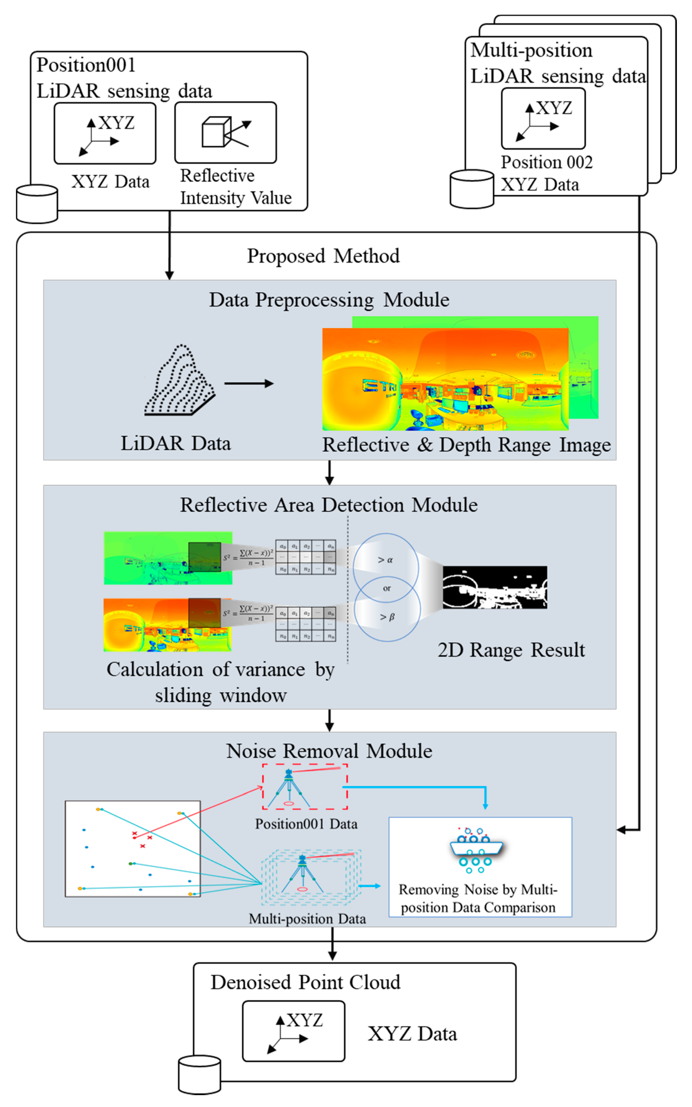
Figure 4.
Point cloud to range image schematic. The red dot in the figure represents part of the point cloud data, and the range image can be obtained by topology expansion.
Figure 4.
Point cloud to range image schematic. The red dot in the figure represents part of the point cloud data, and the range image can be obtained by topology expansion.

Figure 5.
Data preprocessing module overview.

Figure 6.
Examples of reflective range images and depth range images. (a) is the depth range image, (b) is the reflection range image, and (c) is the RGB image.
Figure 6.
Examples of reflective range images and depth range images. (a) is the depth range image, (b) is the reflection range image, and (c) is the RGB image.
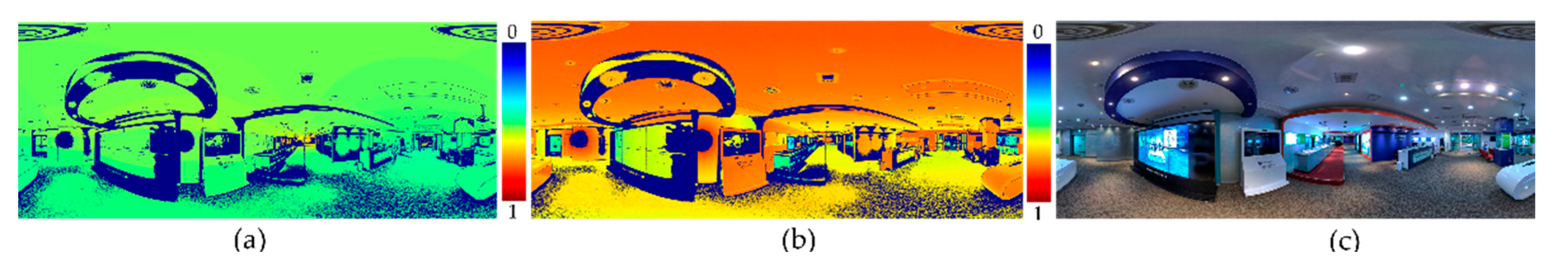
Figure 7.
Point cloud to range image schematic. The red dot in the figure represents part of the point cloud data, and the range image can be obtained by topology expansion.
Figure 7.
Point cloud to range image schematic. The red dot in the figure represents part of the point cloud data, and the range image can be obtained by topology expansion.

Figure 8.
Overview of the variance-based sliding window approach.

Figure 9.
Schematic of the position of points in different sensors.

Figure 10.
Overview of the noise removal module.

Figure 11.
Overview based on the scattered peripheral sensor selection method.

Figure 12.
Overview of the ground truth.

Figure 13.
Noise detection results obtained using our method on single sensor data. (a) is the original point cloud image; (b) is the RGB image and the 2-D result map obtained by using our method; (c) is the obtained reflection noise region, the purple part of the figure; and (d) is the reflection noise region in another view.

Figure 14.
Comparison of our proposed method result and ground truth. (a) is the original point cloud, (b) is the noise detection result, the purple part of the figure, (c) is the point cloud after denoising using our method, and (d) is ground truth data by manual denoising.
Figure 14.
Comparison of our proposed method result and ground truth. (a) is the original point cloud, (b) is the noise detection result, the purple part of the figure, (c) is the point cloud after denoising using our method, and (d) is ground truth data by manual denoising.
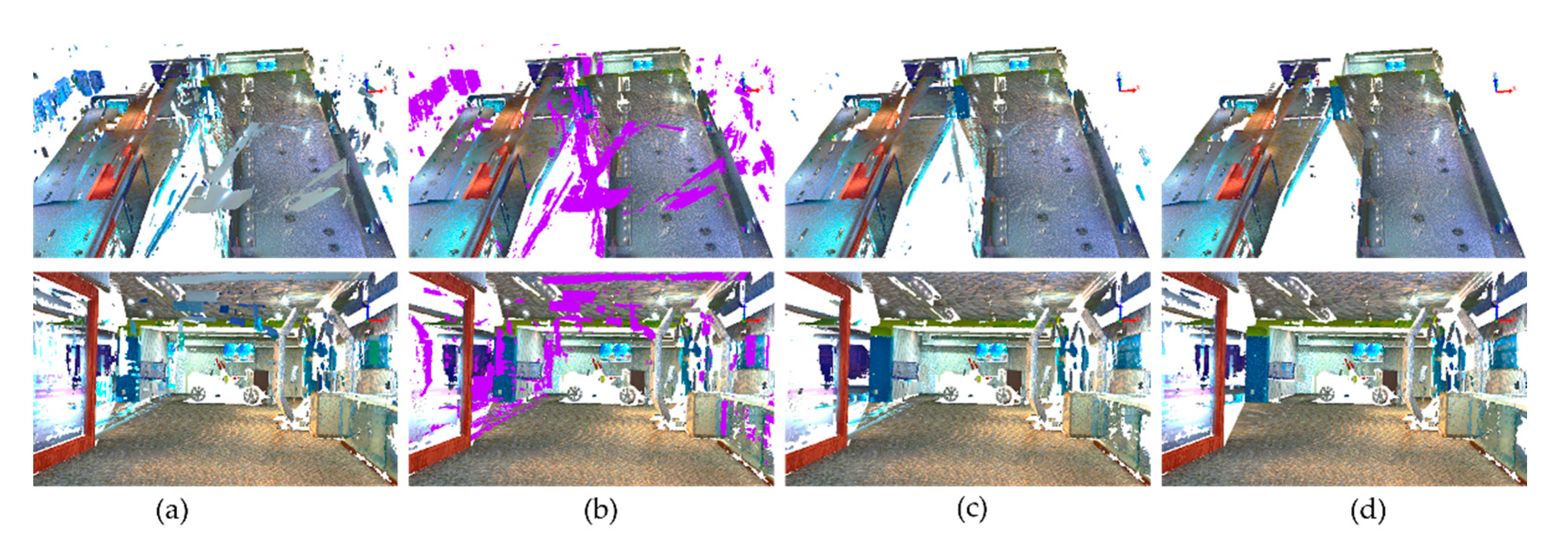
Figure 15.
Description of the noise detection result of each single sensor data and merged result. (a–c) are the noise detection results of sensors 1, 2, and 3, respectively. (d) is the noise detection result using multiple sensor data that are a combined result of (a–c).
Figure 15.
Description of the noise detection result of each single sensor data and merged result. (a–c) are the noise detection results of sensors 1, 2, and 3, respectively. (d) is the noise detection result using multiple sensor data that are a combined result of (a–c).

Figure 16.
Results of the proposed method. (a) is the original point cloud image, (b) the green part of the figure is the reflected noise region detected by our method, and (c) is the result obtained after denoising using our method.
Figure 16.
Results of the proposed method. (a) is the original point cloud image, (b) the green part of the figure is the reflected noise region detected by our method, and (c) is the result obtained after denoising using our method.

Figure 17.
Comparison of the reflective noise results. (a) is the original point cloud image, (b) is the result after processing by FARO SENCE filter, and (c) is the result obtained by our method.
Figure 17.
Comparison of the reflective noise results. (a) is the original point cloud image, (b) is the result after processing by FARO SENCE filter, and (c) is the result obtained by our method.

Figure 18.
Results of the proposed method using different datasets. (a) is the original point cloud image, (b) the green part of the figure is the reflected noise region detected by our method, and (c) is the result obtained after denoising using our method.
Figure 18.
Results of the proposed method using different datasets. (a) is the original point cloud image, (b) the green part of the figure is the reflected noise region detected by our method, and (c) is the result obtained after denoising using our method.


Table 1.
Scanner settings parameters.
| Scanner Settings Name | Parameters |
|---|---|
| Scan Angular Area (Vertical) | |
| Scan Angular Area (Horizontal) | |
| Resolutions | |
| Scanner Distance Range | 130 m |
| Horizontal Motor Speed Factor | 1.02 |
Table 2.
FARO SCENE filter parameters.
| Filter Name | Parameters Name | Parameters |
|---|---|---|
| Proposed Method | Sliding window size | 100 |
| Stride | 50 | |
| Depth variance threshold | 0.2 | |
| Reflection variance threshold | 10,000 | |
| Threshold of deletes nearest sensor γ | 4 | |
| Matching point threshold δ | 1 | |
| Nearest neighbor number ε | 8 | |
| Radius distance ζ | 0.01 | |
| FARO Dark Scan Point Filter | Reflectance Threshold | 900 |
| FARO Distance Filter | Minimum Distance | 0 |
| Maximum Distance | 200 | |
| FARO Stray Point Filter | Grid Size | 3 px |
| Distance Threshold | 0.02 | |
| Allocation Threshold | 50% |
Table 3.
Point number of point cloud.
| Sensors Number | The Size of Range Image | Total Number of Point Cloud | Total Number of Noise Point |
|---|---|---|---|
| S001 | 4268 | 44,088,440 | 128,601 |
| S002 | 4268 | 44,088,440 | 139,343 |
| S003 | 4268 | 44,122,584 | 80,130 |
| S004 | 4268 | 44,088,440 | 128,456 |
| S005 | 4268 | 44,122,584 | 178,147 |
| S006 | 4268 | 44,079,904 | 412,792 |
| S007 | 4268 | 44,088,440 | 283,019 |
| S008 | 4268 | 44,088,440 | 133,439 |
| S009 | 4268 | 44,088,440 | 42,168 |
| S010 | 4268 | 44,088,440 | 109,443 |
| S011 | 4268 | 44,114,048 | 137,085 |
| S012 | 4268 | 44,096,976 | 69,148 |
| S013 | 4268 | 44,088,440 | 77,341 |
| S014 | 4268 | 44,105,512 | 132,483 |
| S015 | 4268 | 44,088,440 | 98,729 |
Table 4.
Comparison of accuracy performance.
| Sensors Number | Accuracy (the Higher, the Better) | |
|---|---|---|
| FARO Result | Our Result | |
| S001 | 0.95351 | 0.97139 |
| S002 | 0.93753 | 0.98322 |
| S003 | 0.94718 | 0.98905 |
| S004 | 0.95088 | 0.99058 |
| S005 | 0.93813 | 0.98503 |
| S006 | 0.92625 | 0.98012 |
| S007 | 0.93602 | 0.98734 |
| S008 | 0.94119 | 0.98779 |
| S009 | 0.94173 | 0.98412 |
| S010 | 0.93568 | 0.98917 |
| S011 | 0.94076 | 0.98981 |
| S012 | 0.95078 | 0.97774 |
| S013 | 0.94661 | 0.97318 |
| S014 | 0.93407 | 0.97917 |
| S015 | 0.94165 | 0.98947 |
| average | 0.94146 | 0.98381 |
Table 5.
Comparison of the quantitative performance.
| Sensors Number | ODR | IDR | FPR | FNR | ||||
|---|---|---|---|---|---|---|---|---|
| FARO Result | Our Result | FARO Result | Our Result | FARO Result | Our Result | FARO Result | Our Result | |
| S001 | 0.16994 | 0.55673 | 0.95580 | 0.97261 | 0.04419 | 0.02738 | 0.83005 | 0.44326 |
| S002 | 0.18977 | 0.69611 | 0.93990 | 0.98413 | 0.06009 | 0.01586 | 0.81022 | 0.30389 |
| S003 | 0.23453 | 0.86457 | 0.94847 | 0.98928 | 0.05152 | 0.01071 | 0.76546 | 0.13543 |
| S004 | 0.22589 | 0.79470 | 0.95300 | 0.99115 | 0.04699 | 0.00884 | 0.77410 | 0.20530 |
| S005 | 0.18062 | 0.80563 | 0.94121 | 0.98576 | 0.05879 | 0.01423 | 0.81938 | 0.19436 |
| S006 | 0.14959 | 0.72257 | 0.93359 | 0.98256 | 0.06640 | 0.01744 | 0.85040 | 0.27742 |
| S007 | 0.15795 | 0.65505 | 0.94104 | 0.98948 | 0.05895 | 0.01051 | 0.84204 | 0.34494 |
| S008 | 0.12123 | 0.82198 | 0.94368 | 0.98829 | 0.05631 | 0.01170 | 0.87876 | 0.17801 |
| S009 | 0.16194 | 0.84753 | 0.94248 | 0.98425 | 0.05751 | 0.01574 | 0.83805 | 0.15246 |
| S010 | 0.05995 | 0.76042 | 0.93785 | 0.98974 | 0.06214 | 0.01025 | 0.94004 | 0.23957 |
| S011 | 0.05431 | 0.84133 | 0.94353 | 0.99027 | 0.05647 | 0.00972 | 0.94568 | 0.15866 |
| S012 | 0.16055 | 0.89068 | 0.95203 | 0.97788 | 0.04797 | 0.02211 | 0.83944 | 0.10931 |
| S013 | 0.11603 | 0.82901 | 0.94807 | 0.97344 | 0.05192 | 0.02656 | 0.88396 | 0.17098 |
| S014 | 0.22899 | 0.80661 | 0.93619 | 0.97969 | 0.06380 | 0.02031 | 0.77100 | 0.19338 |
| S015 | 0.18443 | 0.79391 | 0.94335 | 0.98991 | 0.05664 | 0.01008 | 0.81556 | 0.20608 |
| average | 0.15971 | 0.77912 | 0.94401 | 0.98456 | 0.05597 | 0.01542 | 0.84027 | 0.22087 |
Publisher’s Note: MDPI stays neutral with regard to jurisdictional claims in published maps and institutional affiliations. |
© 2021 by the authors. Licensee MDPI, Basel, Switzerland. This article is an open access article distributed under the terms and conditions of the Creative Commons Attribution (CC BY) license (https://creativecommons.org/licenses/by/4.0/).
Share and Cite
MDPI and ACS Style
Gao, R.; Park, J.; Hu, X.; Yang, S.; Cho, K. Reflective Noise Filtering of Large-Scale Point Cloud Using Multi-Position LiDAR Sensing Data. Remote Sens. 2021, 13, 3058. https://0-doi-org.brum.beds.ac.uk/10.3390/rs13163058
AMA Style
Gao R, Park J, Hu X, Yang S, Cho K. Reflective Noise Filtering of Large-Scale Point Cloud Using Multi-Position LiDAR Sensing Data. Remote Sensing. 2021; 13(16):3058. https://0-doi-org.brum.beds.ac.uk/10.3390/rs13163058
Chicago/Turabian StyleGao, Rui, Jisun Park, Xiaohang Hu, Seungjun Yang, and Kyungeun Cho. 2021. "Reflective Noise Filtering of Large-Scale Point Cloud Using Multi-Position LiDAR Sensing Data" Remote Sensing 13, no. 16: 3058. https://0-doi-org.brum.beds.ac.uk/10.3390/rs13163058
Note that from the first issue of 2016, this journal uses article numbers instead of page numbers. See further details here.