
Estimation of Terrestrial Water Storage Changes at Small Basin Scales Based on Multi-Source Data


1
School of Geography and Information Engineering, China University of Geosciences (Wuhan), Wuhan 430078, China
2
Artificial Intelligence School, Wuchang University of Technology, Wuhan 430223, China
3
State Key Laboratory of Remote Sensing Science, Aerospace Information Research Institute, Chinese Academy of Sciences, Beijing 100101, China
*
Author to whom correspondence should be addressed.
Remote Sens. 2021, 13(16), 3304; https://0-doi-org.brum.beds.ac.uk/10.3390/rs13163304
Submission received: 1 July 2021
/
Revised: 13 August 2021
/
Accepted: 17 August 2021
/
Published: 20 August 2021
(This article belongs to the Special Issue Satellite Hydrological Data Products and Their Applications)
Abstract
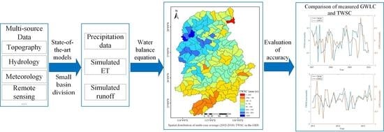
:Terrestrial water storage changes (TWSCs) retrieved from the Gravity Recovery and Climate Experiment (GRACE) satellite mission have been extensively evaluated in previous studies over large basin scales. However, monitoring the TWSC at small basin scales is still poorly understood. This study presented a new method for calculating TWSCs at the small basin scales based on the water balance equation, using hydrometeorological and multi-source data. First, the basin was divided into several sub-basins through the slope runoff simulation algorithm. Secondly, we simulated the evapotranspiration (ET) and outbound runoff of each sub-basin using the PML_V2 and SWAT. Lastly, through the water balance equation, the TWSC of each sub-basin was obtained. Based on the estimated results, we analyzed the temporal and spatial variations in precipitation, ET, outbound runoff, and TWSC in the Ganjiang River Basin (GRB) from 2002 to 2018. The results showed that by comparing with GRACE products, in situ groundwater levels data, and soil moisture storage, the TWSC calculated by this study is in good agreement with these three data. During the study period, the spatial and temporal variations in precipitation and runoff in the GRB were similar, with a minimum in 2011 and maximum in 2016. The annual ET changed gently, while the TWSC fluctuated greatly. The findings of this study could provide some new information for improving the estimate of the TWSC at small basin scales.
1. Introduction
Terrestrial water storage (TWS) is the sum of all forms of water storage over land surfaces and plays a vital role in the global and regional hydrological cycle [1,2,3]. It reflects all types of water stored on continents, including surface water, soil water, and groundwater [4]. TWS change (TWSC) has significant impacts on terrestrial ecosystems, human beings, and even the sea level [5]. Monitoring the spatial and temporal variabilities in TWSC is of great importance for effective water resources management and sustainable utilization [6].
The launch of the Gravity Recovery and Climate Experiment (GRACE) satellites has provided a new method for terrestrial hydrology research, which can efficiently improve the monitoring result of the changes in the water cycle at a large scale [7]. Numerous studies have shown that GRACE satellites play a key role in the large-scale monitoring of TWSC or TWS anomalies (TWSA) [8,9,10]. However, the applications of GRACE satellites are limited by the low spatial resolution that cannot be directly used in small-scale research [11,12,13]. To use GRACE data at small basins, some studies have derived TWS at small basin scales by downscaling GRACE data [14,15,16]. There are two typical types of methods to downscale GRACE data: statistical downscaling and dynamic downscaling. Scholars have used statistical downscaling to establish observed spatial and temporal relationships between GRACE data and inputs (dependent variables such as precipitation, soil moisture, runoff, ET, and so on) using coarse-scale datasets and have applied the established relationships and fine-scale input data to produce the TWS data at small scales [17,18,19]. The major limitation of the statistical downscaling method comes from the assumption of stationarity between the coarse-scale and fine-scale dynamics and from the uncertainty and probability associated with this assumption [20]. In terms of dynamic downscaling methods, many scholars have assimilated GRACE data into the land surface model to obtain high-resolution TWS data [14,21,22]. However, the construction of the dynamic downscaling model is based on defined physical relationships, is physically based but computationally expensive, and is strongly dependent on boundary conditions, and the calculation is relatively complicated; the theoretical model often causes large errors [20].
In recent years, the application of hydrological models has been greatly expanded, which can be further used to estimate small-scale TWSC. In addition to runoff simulations, hydrological models are also used to simulate evapotranspiration (ET), soil moisture, and other water balance components. The hydrological models are effective tools for linking the water balance of the basin with runoff and other hydrological processes. The hydrological models can be divided into empirical models, conceptual models, and physically based models. Empirical models only obtain information from existing data without considering the characteristics and processes of the hydrological system, so these models are only effective within the boundary. The conceptual model uses a semi-empirical equation, and a large amount of in situ data are required for calibration. Calibration involves curve fitting, which makes interpretation difficult, so the effects of land-use change cannot be predicted with great confidence. While the physically based model can overcome many of the shortcomings of the other two models due to the use of parameters with a physical interpretation, it can provide a large amount of information even outside the boundaries and can be applied to a variety of situations [23]. Several studies have used remote sensing and in situ data based on water balance equations, combined with ET and runoff output from various hydrological models, to estimate TWSC at grid scales [24,25,26]. However, as Srivastava et al. [24] mentioned, this method may be suitable for the regions where in situ data are lacking or unavailable. In the regions with relatively more in situ data, e.g., this study, we can make full use of more in situ data to further improve the estimate accuracy. In addition, as a relatively independent catchment unit, the sub-basin can clearly reflect the hydrological processes within and between units. Therefore, studying TWSC at the sub-basin scale can better reflect the TWSC variation pattern.
Hence, in this study, we took the Ganjiang River Basin (GRB) as a case, divided the GRB into several sub-basins, and applied multi-source data, i.e., topography, hydrology, meteorology, and remote sensing, as the data sources. Based on the water balance equation, ET and runoff were modeled by two state-of-the-art models, and we estimated the TWSC at the sub-basin scale (i.e., ~600 km2). Then, we verified the accuracy of this method through GRACE data, groundwater level data, and soil moisture data. We also analyzed the temporal and spatial variations in precipitation, ET, runoff, and TWSC in the GRB during the study period. Our study is based on the water balance and focuses more on the hydrological mechanism compared with the common methods. It is essential to understand the distribution of water resources, flood prevention, and disaster reduction at local scales (county levels), and provide scientific and accurate data support for water resource surveys in small-scale basins.
2. Materials
2.1. Study Area
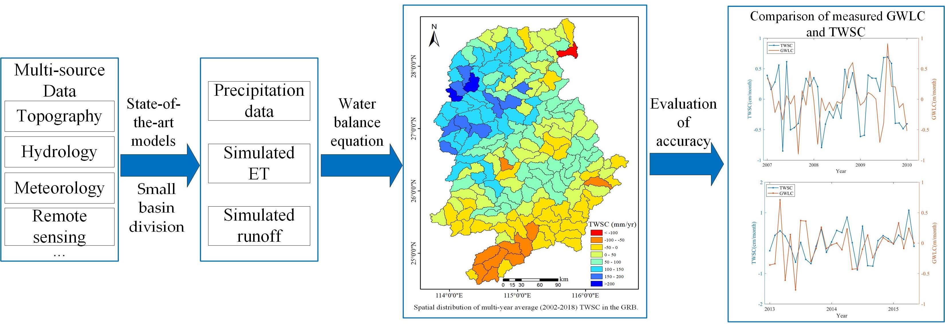
The GRB is the seventh-largest tributary of the Yangtze River, located in the range of 113°30′–116°40′E and 24°29′–29°21′N, as shown in Figure 1. The elevation of the GRB ranges from 5 to 2015 m. The total area of the basin is about 8.09 × 10⁴ km2. With a mild climate and abundant precipitation, the GRB belongs to the subtropical moist monsoon climate area and is one of the typical rainstorm areas in China. As the joint effects of the complex terrain and the East Asian monsoon climate, flood disasters frequently occur in the GRB [27]. The mean annual air temperature is around 18 ℃. It receives an annual precipitation between 1200 and 1700 mm, and the precipitation distribution is uneven throughout the season. More than 60% of the total precipitation is concentrated from April to September [28].
2.2. Data Description
2.2.1. Hydrometeorological Data
The meteorological and hydrological data used in this study mainly include the China meteorological forcing dataset (CMFD), CMA Land Data Assimilation System Version 2.0 (CLDAS-V2.0), and in situ data.
The CMFD is a near-surface meteorological and environmental reanalysis dataset provided by the Institute of Tibetan Plateau Research at the Chinese Academy of Science [29]. The dataset is based on the Princeton reanalysis data, Global Energy and Water Exchanges-Surface Radiation Budget (GEWEX-SRB), the goal of the Global Land Data Assimilation System (GLDAS), and Tropical Rainfall Measuring Mission (TRMM) data, combined with meteorological data from the China Meteorological Administration (CMA). Meteorological station observation data from 740 stations in the CMA were used to correct systematic departures in the background data. The spatial resolution of CMFD is 0.1° × 0.1° with temporal coverage from 1979 to 2018. The CMFD dataset has been widely used in the hydrometeorological forecasts and hydrological research [30,31,32].
CLDAS-V2.0 has a spatial resolution of 0.0625° × 0.0625° and a temporal resolution of 1 h, covering the whole East Asia region (0°–65°N, 60°–160°E). The CLDAS dataset includes a variety of land-surface forcing data, including precipitation, temperature, shortwave radiation, specific humidity, wind speed, surface pressure, and soil status variables. In addition, the CLDAS-V2.0 dataset was developed by CMA. The soil moisture storage (SMS) starts in April 2017, and the SMS data at 2 m were used as the validation data.
In situ groundwater level data of Ganzhou Hotel station (25.84°N, 114.87°E), Zhangjiawei station (25.84°N, 114.94°E), and Yichun station (27.69°N, 114.29°E) used in our study are from the China Groundwater Level Yearbook from the GEO-Environmental Monitoring Institute. The Ministry of Water Resources provides in situ runoff data.
2.2.2. GRACE Data
This study used the GRACE Mascon product from the Center for Space Research (CSR, the University of Texas at Austin) for validation of the mean TWSC estimate in the GRB. CSR Mascon (CSRM) is available at a spatial grid of 0.25° × 0.25° and monthly temporal resolution (www2.csr.utexas.edu/grace/ accessed on 1 July 2021). More details about this product can be found in Save et al. [33]. This product has been widely used for TWSC estimation at large scales [34,35,36].
2.2.3. Digital Elevation Model (DEM) Data
The global 1 arc-second SRTM V3.0 dataset (SRTMGL1) is a joint product of the National Aeronautics and Space Administration (NASA) and the National Geospatial-intelligence Agency (NGA). The SRTMGL1 product can be downloaded at NASA’s Earth Observing System Data and Information System (EOSDIS) website (http://reverb.echo.nasa.gov/ accessed on 1 July 2021). The World Geodetic System 84 (WGS84) ellipsoid and Earth Gravitational Model 1996 (EGM96) geoid were used in the SRTMGL data products [37]. Several studies have validated the STRMGL1 data and shown that the product has high accuracy in China [38,39]. The SRTMGL1 data in this study were used to divide small-scale basins.
3. Methods
3.1. Division of Small-Scale Basin
The slope runoff simulation algorithm proposed by Ocallaghan et al. [40] is widely used in extracting basin features based on DEM [41,42]. Based on the slope runoff simulation algorithm, the river network information of the GRB is extracted from the SRTMGL1. After the SRTMGL1 data are input into the model, the vector river network data of the basin are first generated by the slope runoff simulation algorithm. The basic principle is to simulate the movement path of real surface water flow to describe the catchment capacity of each pixel in the region. Then, the final river network of the region is the basin part whose cumulative flow is greater than the threshold. Using the regional hydrological station information as a constraint, the closest catchment location to these stations is searched for as the basin outlet in the calculated river network. Through the flow direction data calculated in the slope runoff simulation algorithm, all raster image elements controlled by each outlet are retraced one by one. According to the characteristics of pixel distribution, the small-scale basin data can be obtained by connecting the center points of the outermost grid in turn. In this study, we defined a basin an area of ~600 km2 as a small basin.
It is crucial to select appropriate accuracy evaluation indicators for evaluating the accuracy of small basin divisions. Among the river network accuracy evaluation methods, the match error of river system extraction is a common quantitative index, which is to superimpose the extracted river network with the real river network, calculate the fine polygon area produced by its superimposition, and then calculate its proportion in the total basin area. The calculation equation is shown as follows:
D is the match error of basin system extraction, Ai is the area of the finely divided polygons produced by the superposition of the two river networks, and S is the total area of the basin. The research shows that if D is small, it indicates that the river network is better consistent with the real river network. In general, when D is less than 0.02, the precision is high. When D is less than 0.03, the precision is reasonable. When D is more than 0.03, the precision is poor.
3.2. Simulation of High-Resolution Regional ET
ET is the critical link of the hydrological cycle and an essential part of water balance and energy balance [43]. Therefore, the accurate estimation of ET is very important for estimating the TWSC based on the water balance equation in this study.
In order to obtain high-precision ET in the GRB, we used the Penman–Monteith–Leuning Version 2 (PML_V2) model to simulate ET. The PML_V2 has the following features: (i) a relatively simple structure to estimate the coupling of ET and GPP while retaining reasonable biophysical meaning; (ii) includes the effects of CO2 concentration changes on carbon assimilation and canopy conductance; and (iii) can be applied on regional and large scales easily because it only requires daily meteorological and remote sensing forcing data [44]. Furthermore, by comparing with the ground observation data of 95 global flux stations, this product has higher accuracy and is better than most available ET products [45,46,47].
Although PML_V2 performs well on a global scale, there is still room for improvement at regional scales. The MODIS and GLDAS data were used to produce PML_V2 ET data, but GLDAS data used less ground observation data in China [48,49]. Thus, in order to further improve the accuracy of the modeled ET in China, the input data were changed from GLDAS to CMFD in this study. CMFD has advantages of high precision and wide coverage, and it has been widely used in hydrological research [30,31]. Therefore, we used the PML_V2 model and CMFD dataset to estimate the regional ET for the GRB.
3.3. Simulation of Runoff Based on SWAT Model
Hydrological models are widely used to simulate the runoff process, and many scholars have employed some common models such as the Variable Infiltration Capacity (VIC) model [25,26,50], Soil and Water Assessment Tool (SWAT) model [51,52,53], and Identification of Hydrographs and Components from Rainfall, Evaporation, and Stream (IHACRES) model [50,51] to simulate the runoff in various river basins. However, the condition of each basin is different, especially the difference in climate, which makes the selection of hydrological models critical to the accuracy of runoff simulation [52]. In terms of this issue, Huang et al. [54] evaluated the performance of 9 hydrological models for 12 large-scale river basins around the world. In their conclusions, the SWAT model performs well in simulating runoff in the Yangtze River Basin. Some other studies in the literature have also shown that the SWAT model shows good results in the simulation of runoff in China compared with other models, e.g., the VIC model and Xinanjiang model [55,56,57]. As a physically based model, the SWAT model can simulate the short-term and long-term hydrological process, chemical process, erosion process, soil hydrological cycle, and crop production process of the basin rapidly [23,58]. Compared with other models, the SWAT model can simulate the response of runoff to LUCC in most basins in China more obviously and accurately [55,59]. The SWAT model considers the longitudinal movement of water flow in each small unit and the lateral exchange of water flow between each unit and each other, so it is suitable for the simulation of lateral runoff at small scales. Therefore, the SWAT model was used to estimate the outbound runoff at small-scale basins in this study.
The SWAT model of the GRB was established by using the DEM, soil type, land cover, precipitation, and meteorological data. CN2.mgt and 11 other parameters related to runoff were selected by referring to other studies [59]. SWAT-CUP 2012 was used to obtain the ranges of each parameter and sensitivity order through multiple iterations. The sequential uncertainty fitting (SUFI-2) algorithm was used to update parameter values. Daily precipitation and monthly runoff data in 2002–2011 and 2012–2018 were used for the calibration and validation, respectively. The applicability of the model was evaluated by the Nash–Sutcliffe Efficiency (NSE), coefficient of determination (R²), and Percent Bias (PBIAS) indexes.
3.4. Estimation of TWSC Based on the Water Balance Equation
According to the law of conservation of mass, in the hydrological cycle, for any region and period, the difference between the inflow and the outflow of water must be equal to the change in the water storage, which is known as the basin water balance equation. Therefore, we calculated the terrestrial water flux (the slope of the change in terrestrial water storage over a given period) for the GRB using the basin water balance equation (Equation (2)) based on small-basin-scale precipitation, ET, and runoff. Detailed water balance components are shown in Table 1. The TWSC is obtained by integrating the land water flux.
represents the TWSC for a specific period (t), P represents precipitation, ET represents evapotranspiration, and Q represents runoff.
4. Results
4.1. Small-Scale Basin Division in the GRB
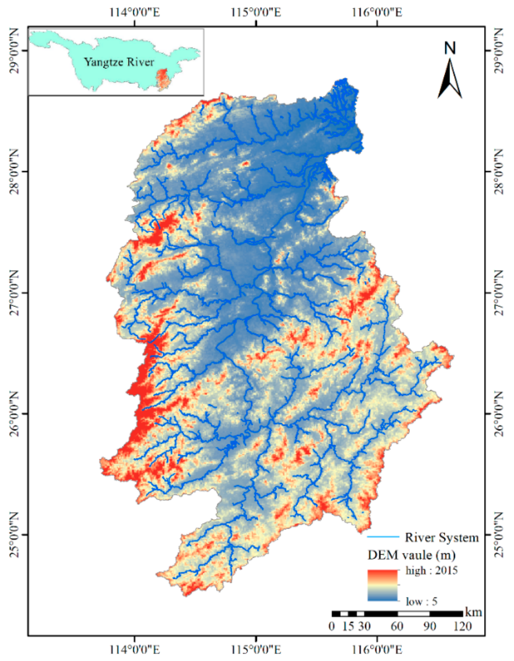
Based on the slope runoff simulation algorithm, the small-scale basin division of the GRB was completed. The small-scale basin division results of the GRB can be divided into two levels. The first level is the control layer of hydrological stations, each hydrological station controls a basin, and the only outlet in the basin is the corresponding hydrological station (as shown in Figure 2a). The second level is the area control layer, subdivided according to the topographic features and river direction based on the first level results. Finally, the GRB is divided into 172 sub-basins, with an average basin area of 591 km2 (as shown in Figure 2b).
Because the real river network information of the GRB is difficult to obtain, our study used the river network data provided by Open Street Map (OSM) to calculate the match error of the extracted river network in the GRB. The results showed that the match error of the extracted river network in our study is 0.013, which meets the accuracy requirement.
4.2. Variation in Precipitation in the GRB
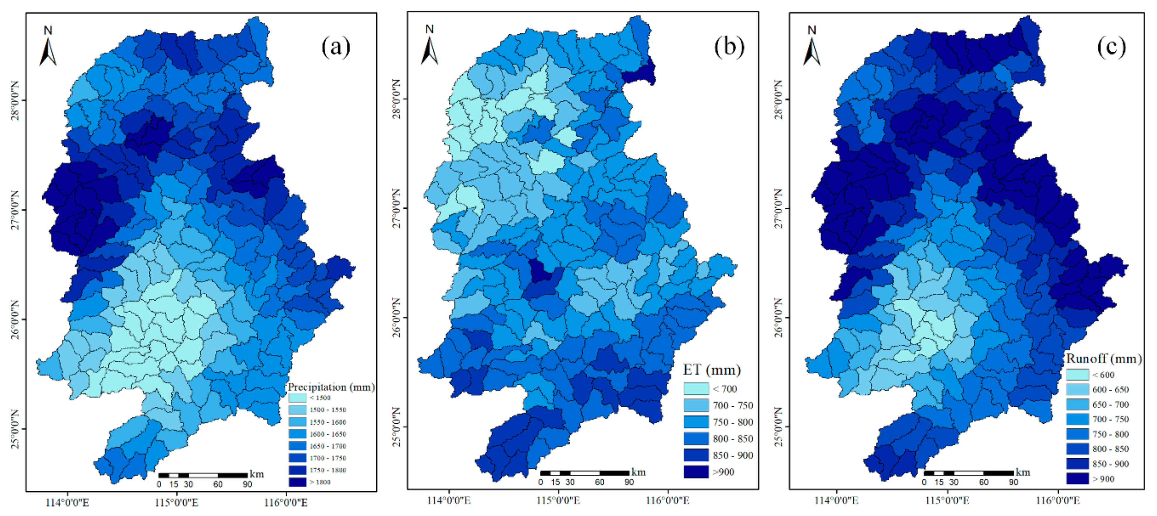
The spatial distribution of average annual precipitation in the GRB from 2002 to 2018 is shown in Figure 3a. The mean annual precipitation of the GRB during the study period ranges from 1500 mm to 1800 mm, with an average value of 1644 mm. The areas with large precipitation are mainly concentrated in the central and northern regions. The precipitation in the central and northern parts of the GRB is more than 1700 mm, while the average annual precipitation in other regions varies from 1500 mm to 1600 mm. Generally speaking, the average annual precipitation is quite different in spatial distribution.
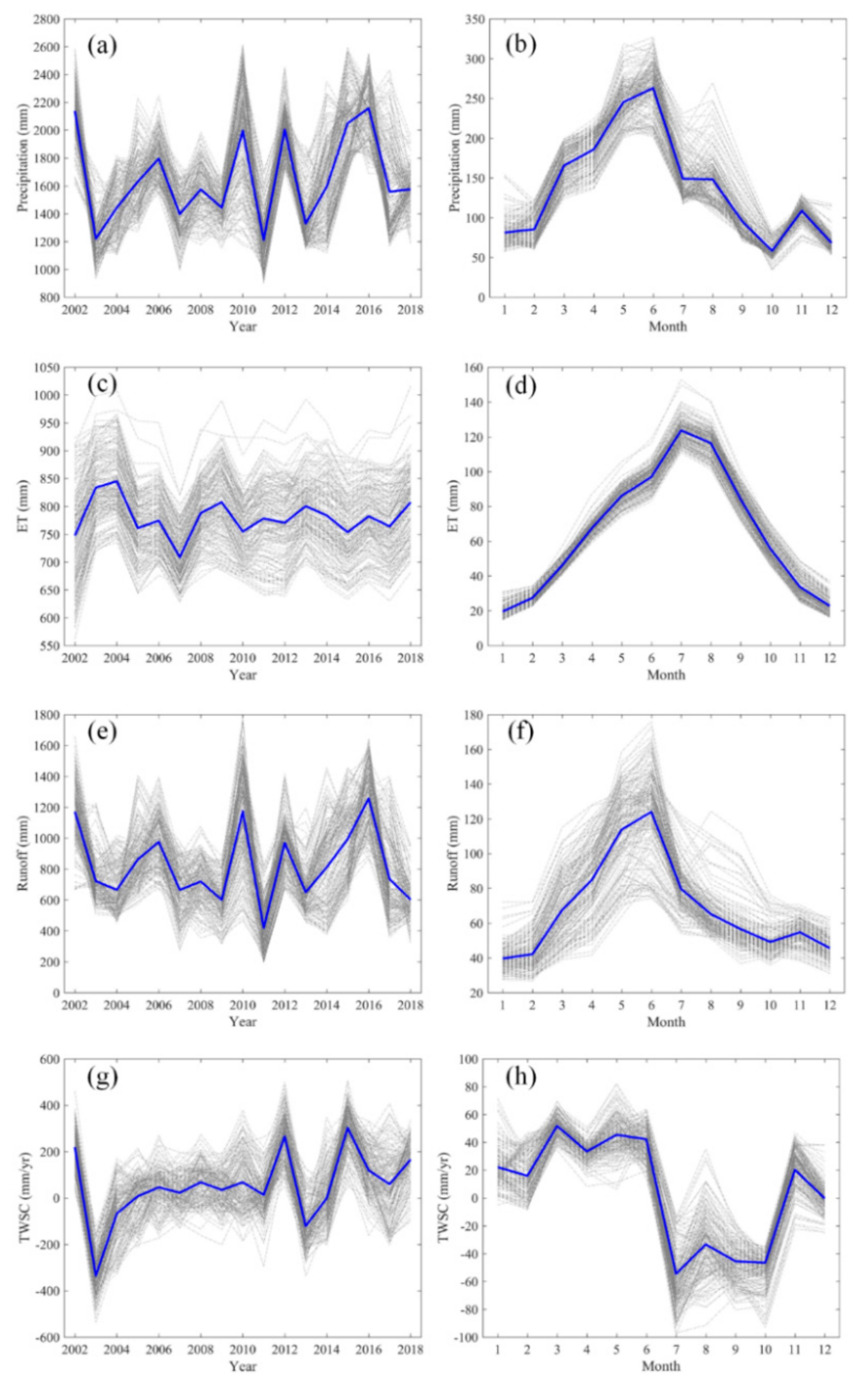
We also calculated the annual and monthly mean precipitation of 172 sub-basins from 2002 to 2018, as shown in Figure 4a,b. Before 2013, the annual precipitation change trend of each sub-basin is relatively consistent, but after 2013, the changing trend of each sub-basin is different. The average standard deviation (STD) values of annual precipitation in 172 sub-basins from 2002 to 2013 is 184.63 mm, and after 2013, it is 240.33 mm. The higher precipitations in most basins occurred in 2002, 2010, 2015, and 2016, and the lower precipitations occurred in 2003, 2007, and 2011. The precipitation in the sub-basins has a large inter-annual variation, and the maximum annual precipitation in the same sub-basin is 2 to 2.5 times that of the minimum annual precipitation.
For the monthly mean precipitation variation of 172 sub-basins in the GRB (Figure 4b), the higher precipitation in most sub-basins occurs in May and June, and the lower precipitation is in October. In May and June with high precipitation, the difference in precipitation in different sub-basins is more than 100 mm. In August, the difference in precipitation between different sub-basins increases further and the difference can reach more than 150 mm. The monthly mean precipitation of different sub-basins varies greatly in the same month. However, the changes in monthly precipitation in the 172 sub-basins of the GRB show a relatively consistent trend during the study period.
4.3. Variation in ET in the GRB
The spatial distribution of the average ET in the GRB from 2002 to 2018 is presented in Figure 3b. Figure 3b shows that the average annual ET of the GRB during the study period varies from 600 mm to 1000 mm, with an average of 780 mm. The regions with maximum ET are concentrated mostly in the middle and south, while the ET in the northwest is lower than those in other regions, and the spatial difference of annual average ET is obvious.
Figure 4c,d show the variation in annual and monthly mean ET in the 172 sub-basins from 2002 to 2018. From Figure 4c, we notice that the ET in most sub-basins presents a relatively consistent fluctuation during the study period, but the annual ET values of different sub-basins in the same year are quite distinct, and the difference in annual ET among the sub-basins can reach 300 mm. Figure 4d shows that the monthly average ET of different sub-basins presents highly consistent fluctuations. The monthly ET increases from January, reaches a peak in July, and then begins to decrease. The average monthly ET of different sub-basins varies from 10 mm to 150 mm. Noting that precipitation and ET show different seasonal variations, the precipitation peaks from May to June, but the peak of ET occurs from July to August, and ET may be affected more by temperature in the GRB.
4.4. Variation in Runoff in the GRB
4.4.1. Validation of Runoff Simulation Accuracy
Figure 5 shows the scatter plots of the simulated and measured monthly runoff data at Waizhou station during the parameter calibration period, with an overall good fitting accuracy and an R2 of 0.88 between the simulated and measured values.
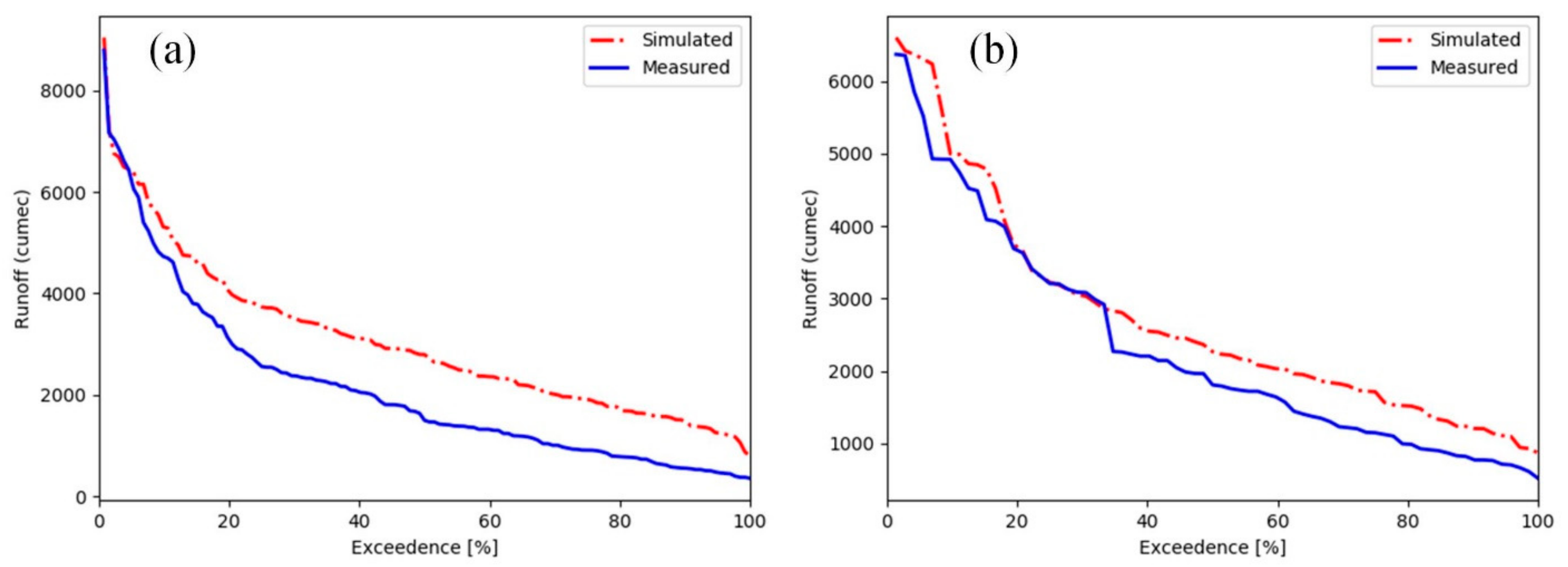
Figure 6 depicts the flow duration curves (FDCs) of the SWAT model at monthly time scales. The variability in the runoff is displayed by the FDC at the Waizhou station for the calibration and validation periods. We can find that the SWAT model simulates the pattern of low, medium, and high runoff satisfactorily at the monthly scale both in the calibration and validation period.
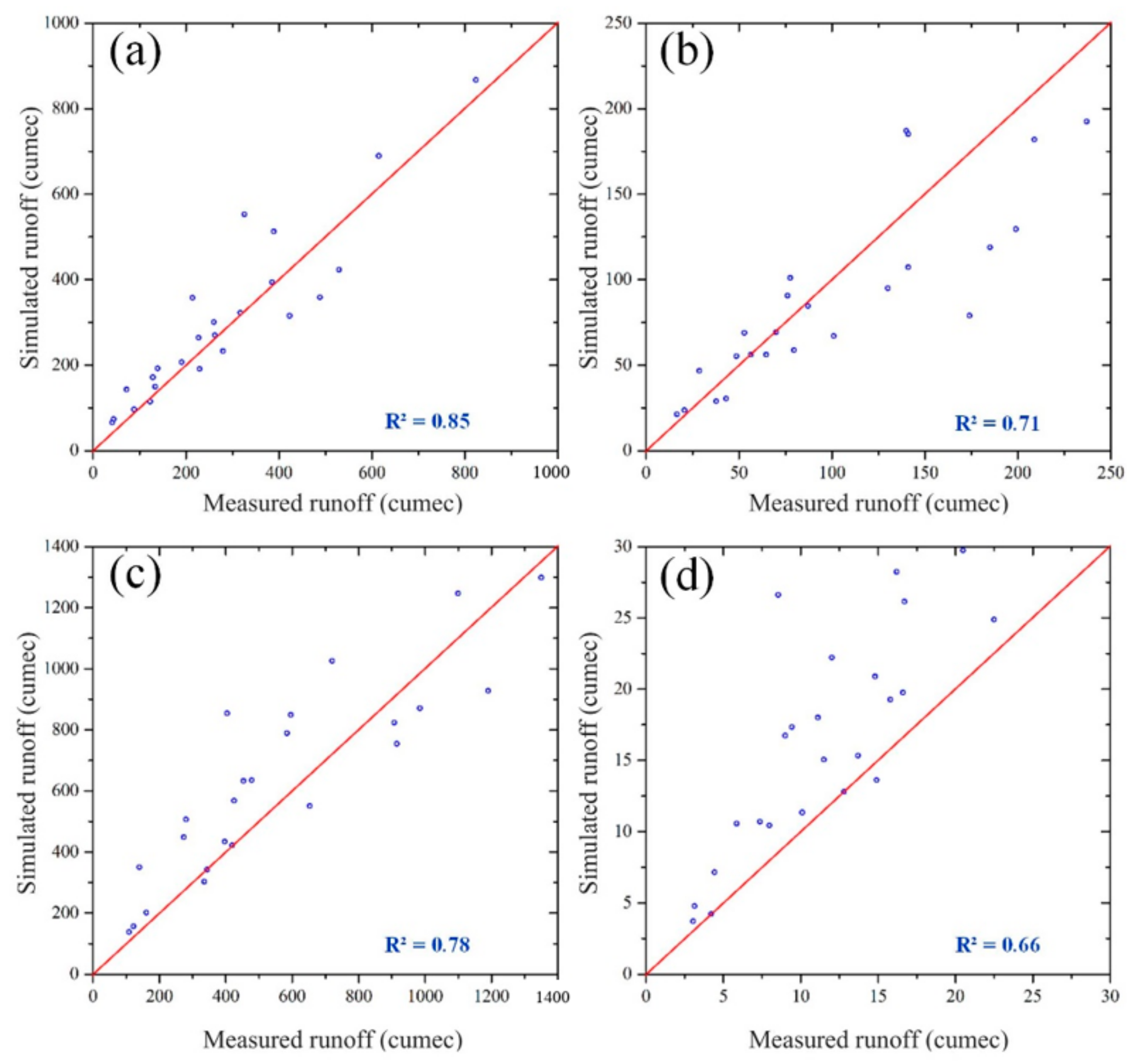
The measured runoff data of Fenkeng station, Hanlinqiao station, Xiashan station, and Junmenling station in 2012 and 2015 were used to further verify the accuracy of the simulated runoff, as shown in Figure 7. The results show that R2 between the modeled and measured runoff ranges from 0.66 to 0.85.
4.4.2. Spatial and Temporal Variation of Runoff
Figure 3c shows the spatial distribution of the annual average runoff at small basin scales in the GRB from 2002 to 2018. The annual average runoff in the GRB ranges from 500 mm to 1100 mm, with an average value of 844 mm. The spatial patterns of runoff are similar to precipitation that gradually increases from the southwest to northeast, and there is a low-value region of runoff in the northwest and a high-value region in the south.
Annual and monthly mean runoff variations in the 172 sub-basins from 2002 to 2018 are presented in Figure 4e,f. The time series of annual mean runoff has good consistencies with precipitation during the study period. The annual runoff of different sub-basins is not completely consistent. However, there is a similar variation rule in 2010 and 2011, with the peak value in 2010 and the valley value in 2011. Precipitation variations from 2010 to 2011 (Figure 4a,b) may cause the runoff changes during the same period. Figure 4f shows the change in monthly average runoff in 172 sub-basins from 2002 to 2018. Overall, it shows an upward trend in the first half of the year, reaches a peak in June, and shows a downward trend in the second half of the year. However, the monthly average runoff in the different sub-basins is quite different, and the difference can reach 100 mm. It should be noted that the seasonal runoff is similar to seasonal precipitation.
4.5. Spatial and Temporal Analysis of TWSC Variation in the GRB
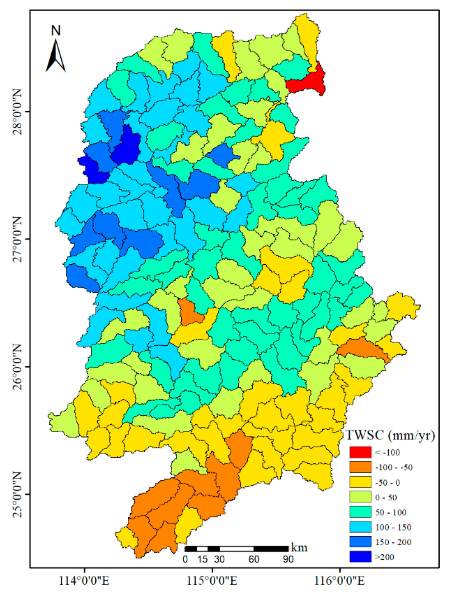
Based on CMFD precipitation, simulated ET, and runoff, we obtained the TWSC estimates of the 172 sub-basins from 2002 to 2018 using the water balance equation. Figure 8 shows the spatial distribution of the average annual TWSC in the GRB from 2002 to 2018. It can be seen from Figure 8 that the TWSC is negative in some areas of the upper reaches, while it is positive in the middle and lower reaches of most sub-basins. One sub-basin in the northeast of the basin has an obvious deficit. Both the largest losses and the largest increases in the TWSC appear in the downstream area.
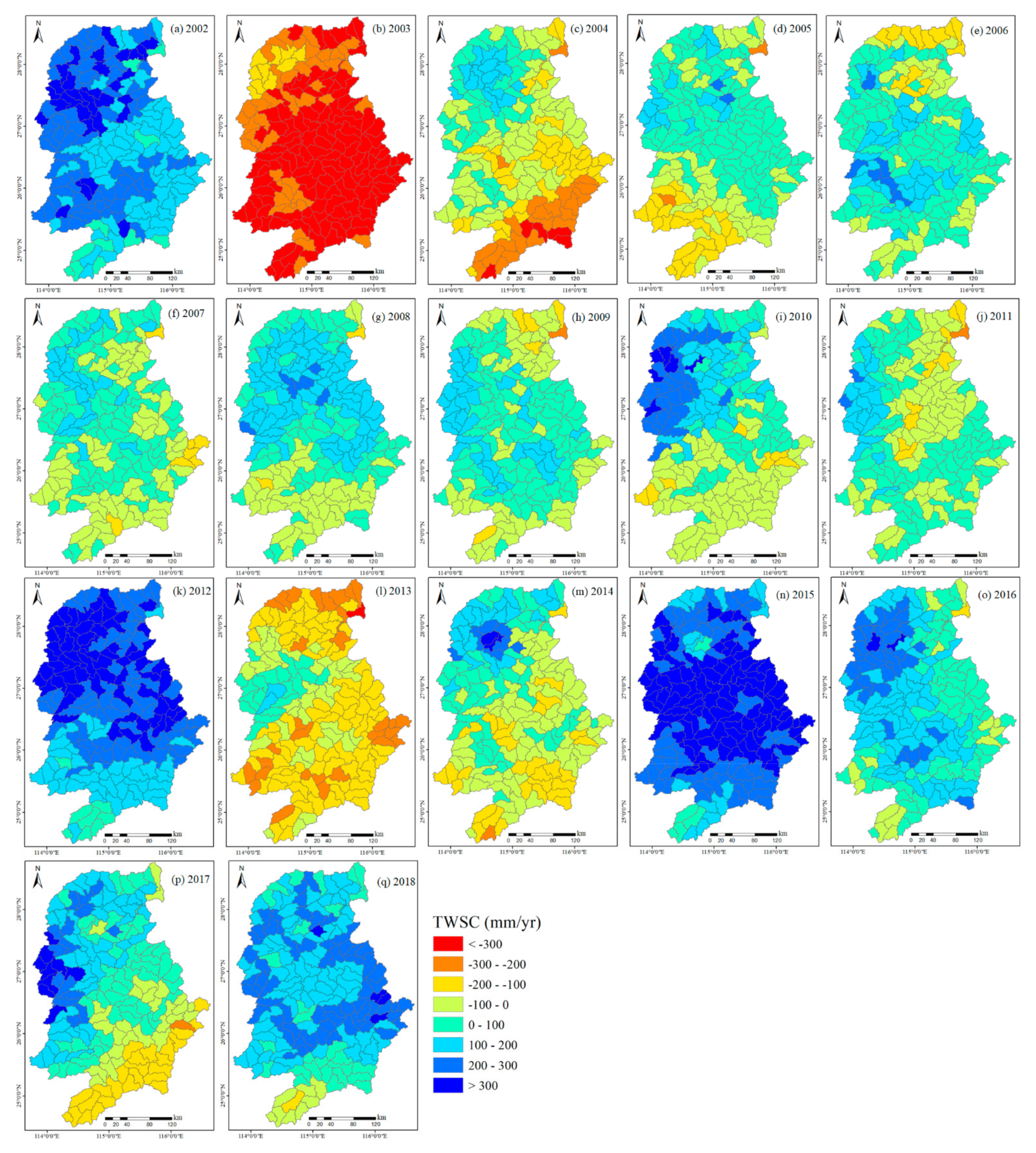
In order to further analyze the variation in TWSC in the GRB, we calculated the spatial distribution of TWSC from 2002 to 2008, as shown in Figure 9. It can be seen that there is a significant loss of TWSC in the GRB in 2003. In 2003, all the TWSC in the GRB shows a negative value, and the loss decreases from the southeast to the northwest. In 2004, the TWSC in the upstream area of the GRB also presents a negative value in most sub-basins. From 2005 to 2009, the TWSC of most sub-basins in the GRB maintains a positive value, but the value is not large. In 2010, the TWSC in the northern part of the GRB increases significantly, while TWSC in the upstream area decreases significantly. In 2012 and 2015, TWSC in the GRB increases significantly, and all sub-basins show an increase in TWSC. In 2013 and 2014, most of the sub-basins manifest a significant loss in TWSC. From 2016 to 2018, most sub-basins in GRB show an increase in TWSC. It should be noted that the interannual variation in TWSC is in good agreement with the interannual variation in precipitation, and the TWSC in the GRB may be more influenced by precipitation.
The time series of annual TWSC in the 172 sub-basins from 2002 to 2018 is shown in Figure 4g. According to the TWSC of 172 sub-basins in different years, it can be seen that the TWSC in most sub-basins show a relatively consistent fluctuation during the study period. TWSC decreases most in 2003, there are obvious increases in 2012 and 2015, and all sub-basins in 2012 and 2015 present positive values in TWSC. Figure 4h shows that in most sub-basins of the GRB, the interannual variation in TWSC is consistent. The monthly mean TWSC in most sub-basins increases from January to June, while the TWSC is in a state of loss from July to October. The difference in TWSC among different sub-basins is large in August but is little in other months. As described in Section 4.2 and Section 4.4, the variations in precipitation and runoff in different sub-basins are also large in August, which may be the reason for the large difference in TWSC.
4.6. Evaluation of Small-Basin-Scale TWSC
4.6.1. Comparison with Other TWSC Data
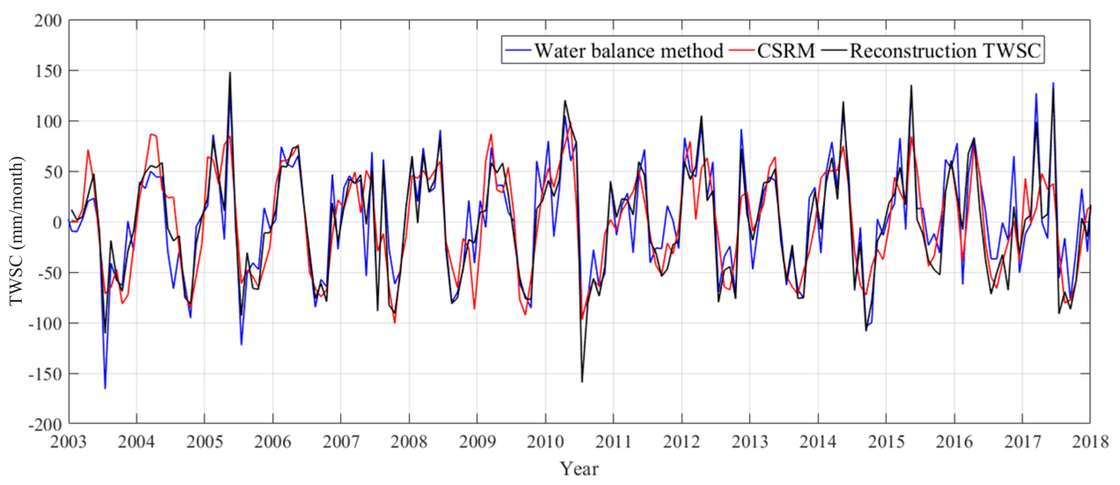
To verify the accuracy of the method in this study, we first compared the TWSC calculated in this study with two TWSC datasets in the whole GRB, considering the coarse resolution of GRACE. The first dataset was the CSRM product. The temporal gaps in CSRM were filled with datasets published by Zhong et al. [60]. With the second data, we used the method proposed by Humphrey et al. [61] to reconstruct the daily TWSA, and further calculated the TWSC of the natural month in the GRB.
Due to the low resolution of GRACE satellites, we evaluated the overall TWSC in the GRB (as shown in Figure 10). The RMSE for the TWSC calculated in this study compared with the CSRM from 2003 to 2018 is 37.1 mm/month. The RMSE between the TWSC calculated in this study and the reconstructed TWSC datasets further reduce to 21.9 mm/month, and the RMSE between CSRM and the reconstructed TWSC is 29.8 mm/month.
4.6.2. Comparison with In Situ Groundwater Level Data
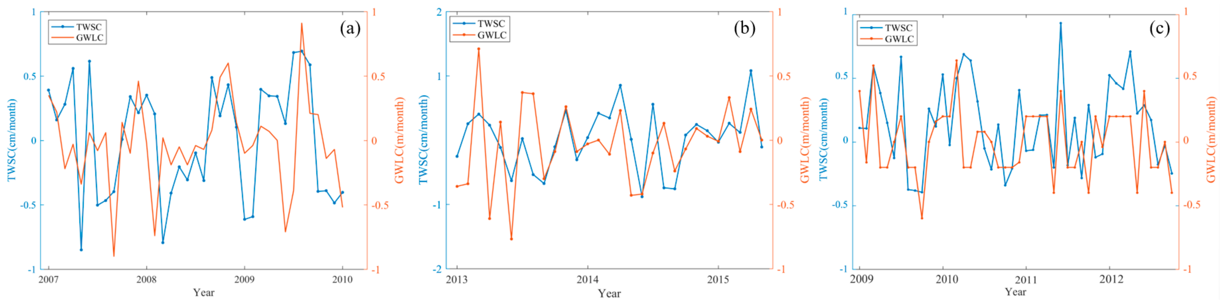
We also used the in situ groundwater level data of the Ganzhou Hotel well site from January 2007 to December 2010, the Zhangjiawei well site from January 2013 to May 2015, and the Yichun well site from January 2009 to December 2012 to verify the TWSC estimates in this study. We compared the Ground Water Level Change (GWLC) with the TWSC estimate in the corresponding sub-basin indirectly, as shown in Figure 11. As a result, the in situ groundwater level data of the three stations and the TWSC of the corresponding sub-basin show a relatively similar variation. However, due to the lack of long time series in situ data, we only analyzed the groundwater level and the TWSC of the corresponding sub-basin of three stations with relatively short time series. In addition, the correlation coefficients (CC) of GWLC and TWSC for all three stations during the analysis period are greater than 0.4.
4.6.3. Comparison with Soil Moisture Storage Change (SMSC)
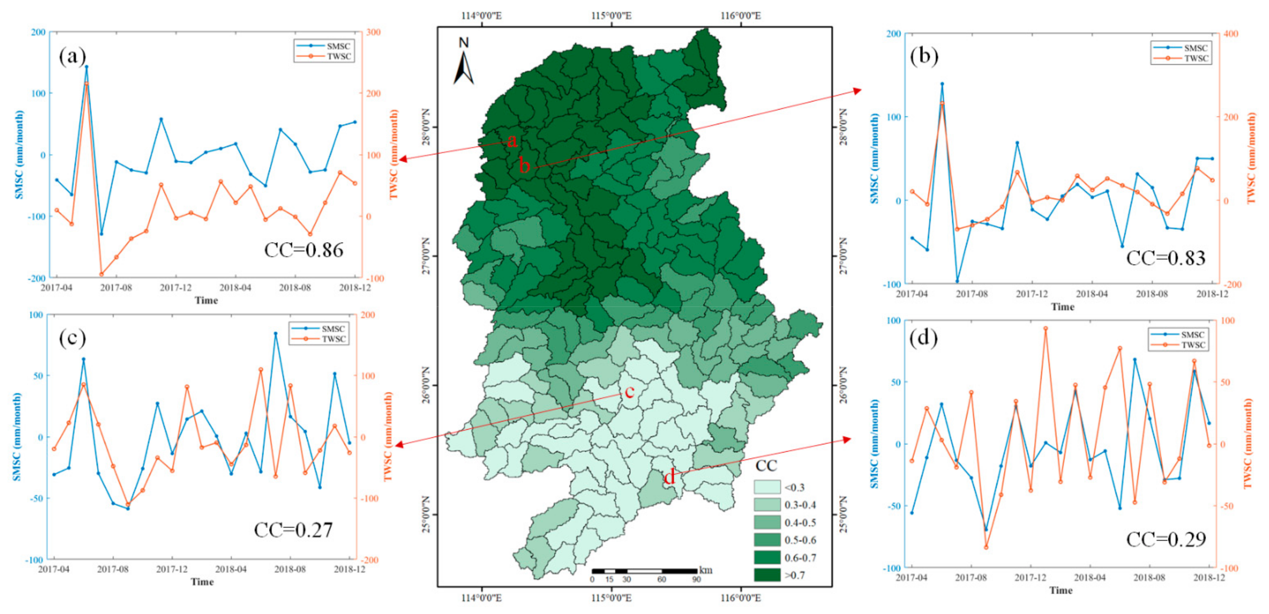
We adopted the CLDAS-V2.0 soil moisture storage (SMS) product to calculate the SMSC of the GRB. Then, SMSC was calculated as the difference between SMS in two consecutive months. We calculated the CC between TWSC and SMSC in 172 sub-basins over the common overlap period (April 2017-December 2018); the spatial distribution is shown in Figure 12. The CC between TWSC and SMSC for 172 sub-basins ranges from 0.26 to 0.88, and the median CC is 0.56. The CC of most sub-basins is greater than 0.5. The sub-basins with larger CC are mainly concentrated in the downstream area, while the sub-basins with smaller CC are mainly concentrated in the upstream area.
Two sub-basins with high CC (labeled (a) and (b)) and two sub-basins with minimum CC (labeled (c) and (d)) were selected for further analysis. It can be seen from Figure 12c,d that although the CC between TWSC and SMSC in these two sub-basins is small, their changes show a relatively good agreement. The most extreme values occurred in the same month. Overall, time series are similar in both data, and the main maxima and minima are found in a similar month. These three comparisons suggest that the TWSC calculated in our study is reliable.
5. Discussion
5.1. Uncertainty
Uncertainties in ET and runoff can come from multiple sources: model misrepresentation or parameterization, forcing data, and other variables [62,63]. Due to the complexity of the model, it is difficult to estimate the uncertainty of ET and runoff caused by the uncertainty of the input precipitation forcing dataset. To quantify the uncertainty of the hydrological model output data, Koukoula et al. [64] evaluated water cycle components from 18 state-of-the-art water resources reanalysis (WRR) datasets derived from different hydrological models, meteorological forcing, and precipitation datasets. They found that the uncertainty in the estimation of the water cycle components from different products is mainly attributable to the differences in the schemes used by the different models, while different precipitation forcing datasets have less impacts on the precision of the WRR output data. Therefore, in this study, we assumed that each variable is independent and estimated the uncertainties of TWSC.
Uncertainties in the monthly estimates of TWSC were assessed by combining the individual uncertainties for precipitation, ET, and runoff with the propagation of errors [65] (Equation (3)).
where , , and represent the error of precipitation, ET, and runoff, respectively.
Due to data limitations, we simply calculated the uncertainties of the TWSC for the whole sub-basins in the GRB. We used monthly precipitation measurements from three precipitation stations in the GRB from the CMA to evaluate the accuracy of the CMFD precipitation estimations. The uncertainty of ET was derived from the RMSE between PML_V2 ET and the ET estimations from the water balance method in the GRB [66]. We used monthly runoff measurements from Waizhou station to evaluate the accuracy of the runoff estimations. The , , , and are ±17.3 mm/month, ±21.2 mm/month, ±28.7 mm/month, and ±39.6 mm/month, respectively. The uncertainty of TWSC estimated with this method is close to the RMSE between the mean TWSC of all sub-basins and TWSC from CSRM in the GRB.
5.2. Impact of ET and Runoff
In the process of ET simulation in small basins, we replaced the forcing data used in the PML_V2 model with the CMFD dataset, but the ET calculated by the PML_V2 model was globally calibrated. There was no region-specific calibration parameter and its accuracy may need further improvement in specific regions at small scales. Zhang et al. [44] showed that when using the PML_V2 model to simulate ET, due to the forcing data of Collection 6 MCD12 has spectral confusion between evergreen broadleaf forests (EBF) and evergreen needleleaf forests (ENF). It is difficult to distinguish several classes using MODIS coarse resolution data, which may lead to some potential uncertainty in ET estimation. Srivastava et al. [24] also showed that due to the MODIS algorithm not considering the effects of cloud cover and leaf shadow effects, MODIS-ET is more accurate in the dry season than in the flood season. The impact of ET by using satellite products also needs to be considered in future research.
We found that the CC between TWSC and SMSC in the sub-basins of the downstream region is generally larger, and the regions with smaller CC are mainly concentrated in the upstream region (Figure 12). It can be seen from Figure 3a,c that the downstream region is also the area with large precipitation and runoff. We speculate that this phenomenon may be related to the accuracy of the runoff simulation. Muleta et al. [67] found that the sensitivity of SWAT model parameters and the accuracy of runoff simulation are significantly different between the periods of high and low precipitation. To address this issue, Levesque et al. [68] applied runoff data from periods of low precipitation to calibrate the SWAT model in a Canadian basin dominated by ice melt recharge and improved the simulation accuracy of the model. In the GRB, there are large spatial differences in precipitation between upstream and downstream regions. However, when we simulated runoff using the SWAT model, the model calibration was carried out for the whole basin due to limited in situ runoff data, which may lead to a higher accuracy of the runoff simulation in the downstream region compared to the upstream region. With more runoff data, we can determine the model parameters from upstream and downstream regions, and further improve the accuracy of the upstream runoff simulation.
Besides, when the SWAT model was applied to simulate the runoff process at a small basin, due to the lack of data about the groundwater process and aquifer system, especially the natural and artificial water storage systems closely related to hydrological conditions, such as dams and reservoirs, wetlands and ponds, the precision is constrained. Kumari et al. [69] also proved that when using the hydrological model to simulate runoff, the shape of a flow duration curve is mainly affected by reservoirs, land-use types, and upstream abstractions of water. The GRB is widely distributed, and several artificial water conservancy facilities such as reservoirs and dams play an important role in the hydrological cycle. If these data are coupled into the model, the accuracy of runoff simulation will be further improved.
6. Conclusions
In this study, we took the GRB as the study area and presented a new method for calculating TWSC at small-basin scales. First, we divided the GRB into 172 sub-basins based on the slope runoff simulation algorithm. Then, we simulated the ET and runoff of each sub-basin with the PML_V2 and SWAT. Finally, through the water balance equation, the TWSC of each sub-basin was obtained. We evaluated its effectiveness by comparing the estimated TWSC against the CSRM, in situ groundwater level data, and SMSC. We also analyzed the temporal and spatial variations in precipitation, ET, runoff, and TWSC in the GRB from 2002 to 2018. From the estimated results and spatio-temporal analyses, we can draw the following conclusions.
The results of this research demonstrate that compared with the in situ data, the simulated runoff is reliable, and the proposed method is capable of obtaining the TWSC at small scales. The TWSC calculated by our method agrees well with the CSRM, in situ groundwater level data, and SMSC. Compared with the CSRM and reconstructed natural monthly TWSC, the RMSE is 37.1 mm/month and 21.9 mm/month, respectively. By comparing with in situ groundwater level data, and SMSC, it shows higher CC. These results indicate that the proposed method makes sense and is beneficial.
The spatial and temporal variations in precipitation and runoff in the GRB are similar, with the minimum value in 2011 and the maximum value in 2016, and the high-value area is mainly concentrated in the downstream area. The annual ET changes gently, with the minimum value in 2007 and the maximum value in 2004. The TWSC fluctuates greatly in the study period, with the minimum value in 2003 and the maximum value in 2015, and the spatial distribution is uniform.
From this study, the accuracy of the evaluation method still needs to be further improved because of the lack of accurate and comparable TWSC observations. We used the GRACE product, the groundwater monitoring level observations, and soil moisture storage to evaluate the method’s accuracy. However, this evaluation method is only qualitative and not quantitative. Nevertheless, we could conclude that in small basins, our method provides reliable data that are suitable for the study of small-basin TWSC. In future work, the quality of the TWSC could be improved by using more accurate runoff and ET simulations.
Author Contributions
Conceptualization, Y.Z., M.W., Q.L. and X.L.; methodology, Y.Z., M.W., Q.L. and S.Z.; data analysis, Y.Z. and Q.L.; validation, Q.L.; writing—original draft preparation, Q.L., Y.Z.; writing—review and editing, Y.Z.; project administration, Y.Z., M.W. and X.L.; funding acquisition, Y.Z., M.W. and X.L. All authors have read and agreed to the published version of the manuscript.
Funding
This research is funded by the Funds of China Geological Survey (No. DD 20190329), National Natural Science Foundation of China (No. 42004073, No. 41974019, and No. 41874091); Fundamental Research Funds for the Central Universities, China University of Geosciences (Wuhan) (No. 26420190050-CUGL190805); and Open Fund of State Key Laboratory of Remote Sensing Science (No.OFSLRSS202107).
Data Availability Statement
The in situ data used in this study were mainly provided by the institution introduced in Section 2.2.1. The China meteorological forcing dataset (CMFD) is available at (http://data.tpdc.ac.cn/en/data/8028b944-daaa-4511-8769-965612652c49/; accessed on 13 August 2021). CMA Land Data Assimilation System Version 2.0 (CLDAS-V2.0) is available at (http://data.cma.cn/data/detail/dataCode/NAFP_CLDAS2.0_NRT/; accessed on 12 August 2021). The GRACE Mascon product from the Center for Space Research is available at (www2.csr.utexas.edu/grace/; accessed on 1 July 2021). The global 1 arc-second SRTM V3.0 dataset (SRTMGL1) is available at (https://lpdaac.usgs.gov/products/srtmgl1v003/; accessed on 1 July 2021). The PML_V2 evapotranspiration is available at (https://code.earthengine.google.com/e0453cf3e7a6e62513da40989f29a029; accessed on 13 August 2021 from GEE). The soil map is available at (http://webarchive.iiasa.ac.at/Research/LUC/External-World-soil-database/HTML/; accessed on 13 August 2021). The dataset used to fill the temporal gaps in the GRACE CSR Mascon product is available at (http://data.tpdc.ac.cn/en/data/71cf70ec-0858-499d-b7f2-63319e1087fc/; accessed on 13 August 2021).
Acknowledgments
We would like to acknowledge the Center for Space Research (CSR), University of Texas at Austin for providing the GRACE mascon solutions. We also thank the China Meteorological Administration (CMA) and the National Tibetan Plateau/Third Pole Environment Data Center (TPDC) for providing the precipitation data.
Conflicts of Interest
The authors declare no conflict of interest.
References
- Zaitchik, B.F.; Rodell, M.; Reichle, R.H. Assimilation of GRACE terrestrial water storage data into a Land Surface Model: Results for the Mississippi River basin. J. Hydrometeorol. 2008, 9, 535–548. [Google Scholar] [CrossRef]
- Long, D.; Longuevergne, L.; Scanlon, B.R. Global analysis of approaches for deriving total water storage changes from GRACE satellites. Water Resour. Res. 2015, 51, 2574–2594. [Google Scholar] [CrossRef] [Green Version]
- Wada, Y.; Wisser, D.; Bierkens, M.F.P. Global modeling of withdrawal, allocation and consumptive use of surface water and groundwater resources. Earth Syst. Dynam. 2014, 5, 15–40. [Google Scholar] [CrossRef] [Green Version]
- Tapley, B.D.; Watkins, M.M.; Flechtner, F.; Reigber, C.; Bettadpur, S.; Rodell, M.; Sasgen, I.; Famiglietti, J.S.; Landerer, F.W.; Chambers, D.P.; et al. Contributions of GRACE to understanding climate change. Nat. Clim. Chang. 2019, 9, 358–369. [Google Scholar] [CrossRef]
- Jiang, D.; Wang, J.; Huang, Y.; Zhou, K.; Ding, X.; Fu, J. The Review of GRACE data applications in terrestrial hydrology monitoring. Adv. Meteorol. 2014, 2014, 725131. [Google Scholar] [CrossRef]
- Seyoum, W.M.; Milewski, A.M. Monitoring and comparison of terrestrial water storage changes in the northern high plains using GRACE and in-situ based integrated hydrologic model estimates. Adv. Water Resour. 2016, 94, 31–44. [Google Scholar] [CrossRef]
- Tapley, B.D.; Bettadpur, S.; Ries, J.C.; Thompson, P.F.; Watkins, M.M. GRACE measurements of mass variability in the Earth system. Science 2004, 305, 503–505. [Google Scholar] [CrossRef] [Green Version]
- Pokhrel, Y.; Felfelani, F.; Satoh, Y.; Boulange, J.; Burek, P.; Gaedeke, A.; Gerten, D.; Gosling, S.N.; Grillakis, M.; Gudmundsson, L.; et al. Global terrestrial water storage and drought severity under climate change. Nat. Clim. Chang. 2021, 11, 226–233. [Google Scholar] [CrossRef]
- Ran, J.; Ditmar, P.; Klees, R.; Farahani, H.H. Statistically optimal estimation of Greenland Ice Sheet mass variations from GRACE monthly solutions using an improved mascon approach. J. Geod. 2018, 92, 299–319. [Google Scholar] [CrossRef] [Green Version]
- Shah, D.; Mishra, V. Strong influence of changes in terrestrial water storage on flood potential in India. J. Geophys. Res. Atmos. 2021, 126, e2020JD033566. [Google Scholar] [CrossRef]
- Zhong, D.; Wang, S.; Li, J. A self-calibration variance-component model for spatial downscaling of GRACE observations using land surface model outputs. Water Resour. Res. 2021, 57, e2020WR028944. [Google Scholar] [CrossRef]
- Chen, L.; He, Q.; Liu, K.; Li, J.; Jing, C. Downscaling of GRACE-derived groundwater storage based on the random forest model. Remote Sens. 2019, 11, 2979. [Google Scholar] [CrossRef] [Green Version]
- Rahaman, M.M.; Thakur, B.; Kalra, A.; Li, R.; Maheshwari, P. Estimating high-resolution groundwater storage from GRACE: A random forest approach. Environments 2019, 6, 63. [Google Scholar] [CrossRef] [Green Version]
- Zhang, D.; Liu, X.; Bai, P. Assessment of hydrological drought and its recovery time for eight tributaries of the Yangtze River (China) based on downscaled GRACE data. J. Hydrol. 2019, 568, 592–603. [Google Scholar] [CrossRef]
- Seyoum, W.M.; Kwon, D.; Milewski, A.M. Downscaling GRACE TWSA data into high-resolution groundwater level anomaly using machine learning-based models in a glacial aquifer system. Remote Sens. 2019, 11, 824. [Google Scholar] [CrossRef] [Green Version]
- Yin, W.; Hu, L.; Zhang, M.; Wang, J.; Han, S. Statistical downscaling of GRACE-derived groundwater storage using ET data in the North China Plain. J. Geophys. Res. Atmos. 2018, 123, 5973–5987. [Google Scholar] [CrossRef]
- Seyoum, W.M.; Milewski, A.M. Improved methods for estimating local terrestrial water dynamics from GRACE in the Northern High Plains. Adv. Water Resour. 2017, 110, 279–290. [Google Scholar] [CrossRef]
- Vishwakarma, B.D.; Zhang, J.; Sneeuw, N. Downscaling GRACE total water storage change using partial least squares regression. Sci. Data 2021, 8, 95. [Google Scholar] [CrossRef] [PubMed]
- Sahour, H.; Sultan, M.; Vazifedan, M.; Abdelmohsen, K.; Karki, S.; Yellich, J.; Gebremichael, E.; Alshehri, F.; Elbayoumi, T. Statistical applications to downscale GRACE-derived terrestrial water storage data and to fill temporal gaps. Remote Sens. 2020, 12, 533. [Google Scholar] [CrossRef] [Green Version]
- Schoof, J.T. Statistical downscaling in climatology. Geogr. Compass 2013, 7, 249–265. [Google Scholar] [CrossRef] [Green Version]
- Khaki, M.; Forootan, E.; Kuhn, M.; Awange, J.; van Dijk, A.I.J.M.; Schumacher, M.; Sharifie, M.A. Determining water storage depletion within Iran by assimilating GRACE data into the W3RA hydrological model. Adv. Water Resour. 2018, 114, 1–18. [Google Scholar] [CrossRef] [Green Version]
- Shokri, A.; Walker, J.P.; van Dijk, A.I.J.M.; Pauwels, V.R.N. Performance of different ensemble kalman filter structures to assimilate GRACE terrestrial water storage estimates into a high-resolution hydrological model: A synthetic study. Water Resour. Res. 2018, 54, 8931–8951. [Google Scholar] [CrossRef]
- Devia, G.K.; Ganasri, B.P.; Dwarakish, G.S. A Review on hydrological models. Aquatic Procedia 2015, 4, 1001–1007. [Google Scholar] [CrossRef]
- Srivastava, A.; Sahoo, B.; Raghuwanshi, N.S.; Singh, R. Evaluation of variable-infiltration capacity Model and MODIS-terra satellite-derived grid-scale evapotranspiration estimates in a river basin with tropical monsoon-type climatology. J. Irrig. Drain. Eng. 2017, 143, 04017028. [Google Scholar] [CrossRef] [Green Version]
- Sridhar, V.; Ali, S.A.; Lakshmi, V. Assessment and validation of total water storage in the Chesapeake Bay watershed using GRACE. J. Hydrol. Reg. Stud. 2019, 24, 100607. [Google Scholar] [CrossRef]
- Xia, Y.; Cosgrove, B.A.; Mitchell, K.E.; Peters-Lidard, C.D.; Ek, M.B.; Brewer, M.; Mocko, D.; Kumar, S.V.; Wei, H.; Meng, J.; et al. Basin-scale assessment of the land surface water budget in the National Centers for Environmental Prediction operational and research NLDAS-2 systems. J. Geophys. Res. Atmos. 2016, 121, 2750–2779. [Google Scholar] [CrossRef] [Green Version]
- Li, N.; Tang, G.; Zhao, P.; Hong, Y.; Gou, Y.; Yang, K. Statistical assessment and hydrological utility of the latest multi-satellite precipitation analysis IMERG in Ganjiang River basin. Atmos. Res. 2017, 183, 212–223. [Google Scholar] [CrossRef]
- Xiao, Y.; Zhang, X.; Wan, H.; Wang, Y.; Liu, C.; Xia, J. Spatial and temporal characteristics of rainfall across Ganjiang River Basin in China. Meteorol. Atmos. Phys. 2016, 128, 167–179. [Google Scholar] [CrossRef]
- He, J.; Yang, K.; Tang, W.; Lu, H.; Qin, J.; Chen, Y.; Li, X. The first high-resolution meteorological forcing dataset for land process studies over China. Sci. Data 2020, 7, 25. [Google Scholar] [CrossRef] [Green Version]
- Shen, M.; Piao, S.; Cong, N.; Zhang, G.; Janssens, I.A. Precipitation impacts on vegetation spring phenology on the Tibetan Plateau. Glob. Chang. Biol. 2015, 21, 3647–3656. [Google Scholar] [CrossRef] [Green Version]
- Hu, Z.; Wang, L.; Wang, Z.; Hong, Y.; Zheng, H. Quantitative assessment of climate and human impacts on surface water resources in a typical semi-arid watershed in the middle reaches of the Yellow River from 1985 to 2006. Int. J. Climatol. 2015, 35, 97–113. [Google Scholar] [CrossRef]
- Han, Y.; Ma, Y.; Wang, Z.; Xie, Z.; Sun, G.; Wang, B.; Ma, W.; Su, R.; Hu, W.; Fan, Y. Variation characteristics of temperature and precipitation on the northern slopes of the Himalaya region from 1979 to 2018. Atmos. Res. 2021, 253, 105481. [Google Scholar] [CrossRef]
- Save, H.; Bettadpur, S.; Tapley, B.D. High-resolution CSR GRACE RL05 mascons. J. Geophys. Res. Solid Earth. 2016, 121, 7547–7569. [Google Scholar] [CrossRef]
- Scanlon, B.R.; Zhang, Z.; Save, H.; Wiese, D.N.; Landerer, F.W.; Long, D.; Longuevergne, L.; Chen, J. Global evaluation of new GRACE mascon products for hydrologic applications. Water Resour. Res. 2016, 52, 9412–9429. [Google Scholar] [CrossRef]
- Zhong, Y.; Zhong, M.; Feng, W.; Zhang, Z.; Shen, Y.; Wu, D. Groundwater depletion in the West Liaohe River Basin, China and its implications revealed by GRACE and in situ measurements. Remote Sens. 2018, 10, 493. [Google Scholar] [CrossRef] [Green Version]
- Zhong, Y.; Feng, W.; Humphrey, V.; Zhong, M. Human-induced and climate-driven contributions to water storage variations in the Haihe River Basin, China. Remote Sens. 2019, 11, 3050. [Google Scholar] [CrossRef] [Green Version]
- Rodriguez, E.; Morris, C.S.; Belz, J.E. A global assessment of the SRTM performance. Photogramm. Eng. Rem. Sens. 2006, 72, 249–260. [Google Scholar] [CrossRef] [Green Version]
- Dong, Y.; Chang, H.; Chen, W.; Zhang, K.; Feng, R. Accuracy assessment of GDEM, SRTM, and DLR-SRTM in Northeastern China. Geocarto Int. 2015, 30, 779–792. [Google Scholar] [CrossRef]
- Jing, C.; Shortridge, A.; Lin, S.; Wu, J. Comparison and validation of SRTM and ASTER GDEM for a subtropical landscape in Southeastern China. Int. J. Digit. Earth. 2014, 7, 969–992. [Google Scholar] [CrossRef]
- Ocallaghan, J.F.; Mark, D.M. The extraction of drainage networks from digital elevation data. Comput. Vision Graph. Image Process. 1984, 28, 323–344. [Google Scholar] [CrossRef]
- Liu, K.; Song, C.; Ke, L.; Jiang, L.; Ma, R. Automatic watershed delineation in the Tibetan endorheic basin: A lake-oriented approach based on digital elevation models. Geomorphology 2020, 358, 107127. [Google Scholar] [CrossRef]
- Stengard, E.; Rasanen, A.; Ferreira, C.S.S.; Kalantari, Z. Inventory and connectivity assessment of wetlands in northern landscapes with a depression-based dem method. Water 2020, 12, 3355. [Google Scholar] [CrossRef]
- Zhang, Y.; Pena-Arancibia, J.L.; McVicar, T.R.; Chiew, F.H.S.; Vaze, J.; Liu, C.; Lu, X.; Zheng, H.; Wang, Y.; Liu, Y.Y.; et al. Multi-decadal trends in global terrestrial evapotranspiration and its components. Sci. Rep. 2016, 6, 19124. [Google Scholar] [CrossRef] [PubMed] [Green Version]
- Zhang, Y.; Kong, D.; Gan, R.; Chiew, F.H.S.; McVicar, T.R.; Zhang, Q.; Yang, Y. Coupled estimation of 500 m and 8-day resolution global evapotranspiration and gross primary production in 2002–2017. Remote Sens. Environ. 2019, 222, 165–182. [Google Scholar] [CrossRef]
- Zhou, R.; Wang, H.; Duan, K.; Liu, B. Diverse responses of vegetation to hydroclimate across temporal scales in a humid subtropical region. J. Hydrol. Reg. Stud. 2021, 33, 100775. [Google Scholar] [CrossRef]
- Elnashar, A.; Zeng, H.; Wu, B.; Zhang, N.; Tian, F.; Zhang, M.; Zhu, W.; Yan, N.; Chen, Z.; Sun, Z.; et al. Downscaling TRMM monthly precipitation using Google Earth engine and Google Cloud Computing. Remote Sens. 2020, 12, 3860. [Google Scholar] [CrossRef]
- Huang, Q.; Qin, G.; Zhang, Y.; Tang, Q.; Liu, C.; Xia, J.; Chiew, F.H.S.; Post, D. Using remote sensing data-based hydrological model calibrations for predicting runoff in ungauged or poorly gauged catchments. Water Resour. Res. 2020, 56, e2020WR028205. [Google Scholar] [CrossRef]
- Wang, W.; Cui, W.; Wang, X.; Chen, X. Evaluation of GLDAS-1 and GLDAS-2 forcing data and Noah Model simulations over China at the monthly scale. J. Hydrometeorol. 2016, 17, 2815–2833. [Google Scholar] [CrossRef]
- Wang, W.; Lin, H.; Chen, N.; Chen, Z. Evaluation of multi-source precipitation products over the Yangtze River Basin. Atmos. Res. 2021, 249, 105287. [Google Scholar] [CrossRef]
- Srivastava, A.; Deb, P.; Kumari, N. Multi-model approach to assess the dynamics of hydrologic components in a tropical ecosystem. Water Resour. Manag. 2020, 34, 327–341. [Google Scholar] [CrossRef]
- Esmali, A.; Golshan, M.; Kavian, A. Investigating the performance of SWAT and IHACRES in simulation streamflow under different climatic regions in Iran. Atmósfera 2020, 34, 79–96. [Google Scholar] [CrossRef] [Green Version]
- Yen, H.; White, M.J.; Jeong, J.; Arabi, M.; Arnold, J.G. Evaluation of alternative surface runoff accounting procedures using SWAT model. Int. J. Agric. Biol. Eng. 2015, 8, 54–68. [Google Scholar]
- Kumar, S.; Singh, A.; Shrestha, D.P. Modelling spatially distributed surface runoff generation using SWAT-VSA: A case study in a watershed of the north-west Himalayan landscape. Model. Earth Syst. Environ. 2016, 2, 1–11. [Google Scholar] [CrossRef] [Green Version]
- Huang, S.; Kumar, R.; Flörke, M.; Yang, T.; Hundecha, Y.; Kraft, P.; Gao, C.; Gelfan, A.; Liersch, S.; Lobanova, A.; et al. Evaluation of an ensemble of regional hydrological models in 12 large-scale river basins worldwide. Clim. Chang. 2017, 141, 381–397. [Google Scholar] [CrossRef]
- Hu, H.C.; Wanga, G.X.; Bi, X.M.; Yang, F.M.; Chongyi, E. Application of two hydrological models to Weihe River basin: A comparison of VIC—3L and SWAT. In SPIE Proceedings [SPIE Geoinformatics 2007—Nanjing, China (Friday 25 May 2007)] Geoinformatics 2007: Remotely Sensed Data and Information; Gong, P., Liu, Y.X., Eds.; SPIE: Bellingham, WA, USA, 2007; Volume 6754. [Google Scholar]
- Li, D.; Qu, S.; Shi, P.; Chen, X.; Xue, F.; Gou, J.; Zhang, W. Development and integration of sub-daily flood modelling capability within the SWAT model and a comparison with XAJ model. Water 2018, 10, 1263. [Google Scholar] [CrossRef] [Green Version]
- Shi, P.; Chen, C.; Srinivasan, R.; Zhang, X.; Cai, T.; Fang, X.; Qu, S.; Chen, X.; Li, Q. Evaluating the SWAT model for hydrological modeling in the Xixian watershed and a comparison with the XAJ model. Water Resour. Manag. 2011, 25, 2595–2612. [Google Scholar] [CrossRef]
- Arnold, J.G.; Moriasi, D.N.; Gassman, P.W.; Abbaspour, K.C.; White, M.J.; Srinivasan, R.; Santhi, C.; Harmel, R.D.; van Griensven, A.; Van Liew, M.W.; et al. Swat: Model use, calibration, and validation. T. Asabe 2012, 55, 1491–1508. [Google Scholar] [CrossRef]
- Luo, X.; Li, J.; Zhu, S.; Xu, Z.; Huo, Z. Estimating the impacts of urbanization in the next 100 years on spatial hydrological response. Water Resour. Manag. 2020, 34, 1673–1692. [Google Scholar] [CrossRef]
- Zhong, Y.; Feng, W.; Zhong, M.; Ming, Z. Dataset of Reconstructed Terrestrial Water Storage in China Based on Precipitation (2002–2019); National Tibetan Plateau Data Center: Beijing, China, 2020. [Google Scholar] [CrossRef]
- Humphrey, V.; Gudmundsson, L. GRACE-REC: A reconstruction of climate-driven water storage changes over the last century. Earth Syst. Sci. Data 2019, 11, 1153–1170. [Google Scholar] [CrossRef] [Green Version]
- Long, D.; Longuevergne, L.; Scanlon, B.R. Uncertainty in evapotranspiration from land surface modeling, remote sensing, and GRACE satellites. Water Resour. Res. 2014, 50, 1131–1151. [Google Scholar] [CrossRef] [Green Version]
- Han, Z.; Long, D.; Huang, Q.; Li, X.; Zhao, F.; Wang, J. Improving reservoir outflow estimation for ungauged basins using satellite observations and a hydrological model. Water Resour. Res. 2020, 56, e2020WR027590. [Google Scholar] [CrossRef]
- Koukoula, M.; Nikolopoulos, E.I.; Dokou, Z.; Anagnostou, E.N. Evaluation of global water resources reanalysis products in the upper Blue Nile River Basin. J. Hydrometeorol. 2020, 21, 935–952. [Google Scholar] [CrossRef] [Green Version]
- Rodell, M.; McWilliams, E.B.; Famiglietti, J.S.; Beaudoing, H.K.; Nigro, J. Estimating evapotranspiration using an observation based terrestrial water budget. Hydrol. Process. 2011, 25, 4082–4092. [Google Scholar] [CrossRef]
- Boronina, A.; Ramillien, G. Application of AVHRR imagery and GRACE measurements for calculation of actual evapotranspiration over the Quaternary aquifer (Lake Chad basin) and validation of groundwater models. J. Hydrol. 2008, 348, 98–109. [Google Scholar] [CrossRef]
- Muleta, M.K. Improving model performance using season-based evaluation. J. Hydrol. Eng. 2012, 17, 191–200. [Google Scholar] [CrossRef]
- Levesque, E.; Anctil, F.; van Griensven, A.; Beauchamp, N. Evaluation of streamflow simulation by SWAT model for two small watersheds under snowmelt and rainfall. Hydrol. Sci. J. 2008, 53, 961–976. [Google Scholar] [CrossRef] [Green Version]
- Kumari, N.; Srivastava, A.; Sahoo, B.; Raghuwanshi, N.S.; Bretreger, D. Identification of suitable hydrological models for streamflow assessment in the Kangsabati River Basin, India, by using different model selection scores. Nat. Resour Res. 2021, 1–19. [Google Scholar] [CrossRef]
Figure 1.
The location of the Ganjiang River Basin and the distribution of river system.

Figure 2.
Results of small-scale basin division in the Ganjiang River Basin (a) the hydrological stations control layer, (b) the area control layer.
Figure 2.
Results of small-scale basin division in the Ganjiang River Basin (a) the hydrological stations control layer, (b) the area control layer.

Figure 3.
Spatial distributions in multi-year average (2002–2018) (a) precipitation, (b) ET, and (c) runoff in the Ganjiang River basin.
Figure 3.
Spatial distributions in multi-year average (2002–2018) (a) precipitation, (b) ET, and (c) runoff in the Ganjiang River basin.

Figure 4.
Annual and monthly mean (a,b) precipitation, (c,d) ET, (e,f) runoff, and (g,h) TWSC variation in the 172 sub-basins from 2002 to 2018 (the blue line represents the average of the 172 sub-basins). The left panel shows annual results and the right panel shows monthly mean results.
Figure 4.
Annual and monthly mean (a,b) precipitation, (c,d) ET, (e,f) runoff, and (g,h) TWSC variation in the 172 sub-basins from 2002 to 2018 (the blue line represents the average of the 172 sub-basins). The left panel shows annual results and the right panel shows monthly mean results.

Figure 5.
Scatter plot of simulated and measured monthly runoff of Waizhou station during calibration period. Note: the cumec represents the unit of runoff in cubic meters per second.
Figure 5.
Scatter plot of simulated and measured monthly runoff of Waizhou station during calibration period. Note: the cumec represents the unit of runoff in cubic meters per second.

Figure 6.
Comparison of flow duration curves of simulated runoff using the SWAT model against observed runoff at Waizhou station: (a) calibration; (b) validation.
Figure 6.
Comparison of flow duration curves of simulated runoff using the SWAT model against observed runoff at Waizhou station: (a) calibration; (b) validation.

Figure 7.
Scatter plot of simulated and measured monthly runoff of (a) Fenkeng station, (b) Hanlinqiao station, (c) Xiashan station, and (d) Junmenling station in 2012 and 2015.
Figure 7.
Scatter plot of simulated and measured monthly runoff of (a) Fenkeng station, (b) Hanlinqiao station, (c) Xiashan station, and (d) Junmenling station in 2012 and 2015.

Figure 8.
Spatial distribution of multi-year average (2002–2018) TWSC in the Ganjiang River Basin.

Figure 9.
Spatial distribution in annual TWSC in the Ganjiang River Basin from 2002 to 2018 (a–q).

Figure 10.
Comparison of TWSC calculated by different methods and CSRM in the Ganjiang River Basin.

Figure 11.
Comparison of measured GWLC and TWSC ((a) Ganzhou Hotel station, (b) Zhangjiawei station, and (c) Yichun station).
Figure 11.
Comparison of measured GWLC and TWSC ((a) Ganzhou Hotel station, (b) Zhangjiawei station, and (c) Yichun station).

Figure 12.
The spatial distribution of the CC between TWSC and SMSC (a,b) time series of two sub-basins with high CC, (c,d) time series of two sub-basins with low CC.
Figure 12.
The spatial distribution of the CC between TWSC and SMSC (a,b) time series of two sub-basins with high CC, (c,d) time series of two sub-basins with low CC.


Table 1.
Detailed water balance components.
| Component | Source | Forcing Data | Temporal Resolution | Spatial Resolution | Reference |
|---|---|---|---|---|---|
| Precipitation (P) | CMFD | GEWEX-SRB, GLDAS, TRMM, Meteorological data from the China Meteorological Administration (CMA) | monthly | 0.1° × 0.1° | He et al., 2019 [29] |
| Evapotranspiration (ET) | PML_V2-simulated | CMFD, MCD15A3H.006, MCD43A3.006, MOD11A2.006, MCD12Q1 | 8 day | 500 m | Zhang et al., 2019 [44] |
| Runoff (Q) | SWAT-simulated | CMFD, SRTMGL1, Land Use/Land Cover Data, Soil map data, Meteorological data from the CMA | monthly | virtual station | Luo et al., 2020 [59] |
Publisher’s Note: MDPI stays neutral with regard to jurisdictional claims in published maps and institutional affiliations. |
© 2021 by the authors. Licensee MDPI, Basel, Switzerland. This article is an open access article distributed under the terms and conditions of the Creative Commons Attribution (CC BY) license (https://creativecommons.org/licenses/by/4.0/).
Share and Cite
MDPI and ACS Style
Li, Q.; Liu, X.; Zhong, Y.; Wang, M.; Zhu, S. Estimation of Terrestrial Water Storage Changes at Small Basin Scales Based on Multi-Source Data. Remote Sens. 2021, 13, 3304. https://0-doi-org.brum.beds.ac.uk/10.3390/rs13163304
AMA Style
Li Q, Liu X, Zhong Y, Wang M, Zhu S. Estimation of Terrestrial Water Storage Changes at Small Basin Scales Based on Multi-Source Data. Remote Sensing. 2021; 13(16):3304. https://0-doi-org.brum.beds.ac.uk/10.3390/rs13163304
Chicago/Turabian StyleLi, Qin, Xiuguo Liu, Yulong Zhong, Mengmeng Wang, and Shuang Zhu. 2021. "Estimation of Terrestrial Water Storage Changes at Small Basin Scales Based on Multi-Source Data" Remote Sensing 13, no. 16: 3304. https://0-doi-org.brum.beds.ac.uk/10.3390/rs13163304
Note that from the first issue of 2016, this journal uses article numbers instead of page numbers. See further details here.