Densely Connected Pyramidal Dilated Convolutional Network for Hyperspectral Image Classification

Abstract

Recently, with the extensive application of deep learning techniques in the hyperspectral image (HSI) field, particularly convolutional neural network (CNN), the research of HSI classification has stepped into a new stage. To avoid the problem that the receptive field of naive convolution is small, the dilated convolution is introduced into the field of HSI classification. However, the dilated convolution usually generates blind spots in the receptive field, resulting in discontinuous spatial information obtained. In order to solve the above problem, a densely connected pyramidal dilated convolutional network (PDCNet) is proposed in this paper. Firstly, a pyramidal dilated convolutional (PDC) layer integrates different numbers of sub-dilated convolutional layers is proposed, where the dilated factor of the sub-dilated convolution increases exponentially, achieving multi-sacle receptive fields. Secondly, the number of sub-dilated convolutional layers increases in a pyramidal pattern with the depth of the network, thereby capturing more comprehensive hyperspectral information in the receptive field. Furthermore, a feature fusion mechanism combining pixel-by-pixel addition and channel stacking is adopted to extract more abstract spectral–spatial features. Finally, in order to reuse the features of the previous layers more effectively, dense connections are applied in densely pyramidal dilated convolutional (DPDC) blocks. Experiments on three well-known HSI datasets indicate that PDCNet proposed in this paper has good classification performance compared with other popular models.

1. Introduction

Hyperspectral remote sensing image is characterized by high dimension, high resolution, and rich spectral and spatial information [1], which have been diffusely used in numerous real-world tasks, such as sea ice detection [2], ecosystem monitoring [3,4], vegetation species analysis [5] and classification tasks [6,7]. With the speedy progress of remote sensing technology and artificial intelligence (AI), a great proportion of new theories and methods in deep learning have been proposed to handle the challenges and problems faced by the field of hyperspectral image [8].

Hyperspectral image classification is an vital branch in the subject of HSI, which has gradually become a crucial direction for scholars in the AI industry. It is worth noting that hyperspectral image pixel-level classification determines the category label of each pixel, and segmentation determines the boundary of a given category of objects. HSI classification and segmentation are related to each other, and segmentation involves the classification of individual pixels. A number of conventional spectral-based classifiers, such as support vector machines (SVM) [9,10], random forest [11,12,13], k-nearest neighbors (kNN) [14,15,16], Bayesian [17], etc., can only show good classification performance in the case of abundant labeled training samples. Recently, more and more methods based on deep learning have been applied to HSI classification tasks, and have achieved well results, for instance, generative adversarial networks (GAN) [18,19,20], recurrent neural networks (RNN) [21,22,23], fully convolutional network (FCN) [24,25,26] and convolution neural network (CNN) [27,28,29]. Among the above methods, the capability of CNN is peculiarly salient. For most image classification issues, CNN is mainly composed of input layer, convolutional layer, pooling layer, fully connected layer and softmax layer. The convolutional layer is the most crucial part of CNN, which consists of multiple hidden layers. Hu et al. designed one-dimensional CNN (1D CNN) to extract feature maps of HSI in the spectral domain [30]. Cao et al. proposed a two-dimensional CNN (2D CNN) based on the active learning method, which reduces cost and improves accuracy by selecting pixels with the largest amount of information for labeling [31]. Hyperspectral images are typically divided into three-dimensional cubes, which makes it possible to classify them with a three-dimensional network structure. Xu et al. suggested a three-dimensional CNN (3-D CNN) framework for effectively extracting HSI information to acquire accurate classification results [27]. Li et al. designed a 3D CNN model combined with regularization to effectively extract the spectral-spatial features of hyperspectral images [32]. In addition, Woo et al. focused on another architecture design, the convolutional block attention module (CBAM), which can learned “what” and “where”, respectively, to enhance the network’s presentation capabilities [33]. Ma et al. proposed a double-branch multi-attention (DBMA) mechanism for HSI classification, and the branches of the network are used to capture more discriminative spectral and spatial features [34]. Li et al. proposed a double-branch dual-attention (DBDA) framework for HSI classification to capture and extract feature information [35].

Generally speaking, one way to obtain better classification results is by increasing the depth of the network. However, vanishing gradient and exploding gradient problems will appear with the increase of network layers, which will lead in the decline of accuracy and network degradation. He et al. proposed a residual network (ResNet) to solve the above problems, which integrates the shallow layer features of the network into subsequent layers through skip connections [36]. Zhong et al. applied the structure of residual blocks in the field of HSI classification and achieved active results [37]. Zhong et al. designed a supervised 3D spectral–spatial residual network (SSRN) to mitigate the decrease in model accuracy [38]. Meng et al. proposed a multipath ResNet (MPRN) framework that makes the network wider to realize effective gradient flow [39]. Inspired by ResNet, Han et al. proposed a novel residual structure, namely pyramidal residual network (PresNet), which can gradually increase the dimension of the feature maps to acquire as much information as possible [40]. Paoletti et al. designed a deep PresNet for HSI classification, which involves more location information as the depth of network increasing [41]. A fully dense multi-scale fusion network (FDMFN) for HSI classification proposed in [42], by fusing multi-scale spectral spatial features, which can obtain active classification results. Another way to improve the performance of the network is by reusing the features of all the previous layers, which can reduce parameters while avoiding the network being too deep or too wide, and alleviate the problem of vanishing gradient to a certain extent. Huang et al. proposed a dense connected network (DenseNet), which establishes a dense connection between all the front layers and back layers to achieve feature reuse on the channel [43]. A mixed link network for HSI classification proposed in [44], by combining the advantages of ResNet and DenseNet, which can further obtain the richer feature information and enhance the network learning ability. Paoletti et al. proposed a novel framework for HSI classification based on DenseNet, which can effectively alleviate overfitting and reduce excessive parameters [45].

In addition, Nalepa et al. proposed a resource-saving quantitative convolutional neural network for hyperspectral image segmentation, in which the quantization process can be well combined with the training process [46]. Moreover, the network can greatly reduce the complexity of the model without affecting the classification accuracy. Fu et al. proposed a super-pixel segmentation algorithm [47]. For high-texture hyperspectral images, the algorithm can decompose them into inhomogeneous blocks, which well maintains the homogeneous characteristic. Sun et al. proposed a fully convolutional segmentation network, which can simultaneously recognize the true labels of all pixels in the HSI cube [48]. For those cubes that contain more land cover categories, it has better recognition capabilities. The DeepLab v3+ network shows active performance in the field of semantic segmentation. Si et al. applied it to the field of HSI image classification for feature extraction [49]. Then, the SVM classifier is used to get the final classification result.

CNN will have better classification performance if the convolutional layer can capture more spectral–spatial information. Although the problem that the receptive field of naive convolution is too small can be effectively solved by dilated convolution, there are unrecognized regions (blind spots) in the receptive field of dilated convolution. Inspired by densely connected multi-dilated DenseNet (D3Net) [50], densely connected pyramidal dilated convolutional network for HSI classification is proposed in this paper to acquired more comprehensive feature information. The structure of the network is composed of several densely pyramidal dilated convolutional blocks and transition layers. In order to increase the size of the receptive field and eliminate blind spots without increasing parameters, dilated convolution with different dilated factors are applied to develop PDC layers. A hybrid feature fusion mechanism is applied to obtain richer information and reduce the depth of the network. The main contributions of the paper are summarized as follows. Firstly, the larger receptive field is obtained by applying the dilated convolution to CNN. Furthermore, in order to avoid blind spots in the receptive field of the feature maps extracted by dilated convolution, we set the dilated factors appropriately and increase the width of the network. Then, the hybrid feature fusion method of pixel-by-pixel addition and channel stacking is applied to extract more abstract feature information while effectively utilizing features. In addition, our network (PDCNet) achieves better performance on well-known datasets (Indian Pines, Pavia University and Salinas Valley datasets) by combining dilated convolution and dense connections than some popular methods.

The remaining part of this paper is organized as follows: Some state-of-the-art technologies related to convolutional neural networks for HSI classification will be introduced in Section 2. In Section 3, methods and network architecture proposed in this paper will be described in detail. The experimental settings and classification results will be shown in Section 4. The discussion of training samples, the number of parameters and the running time of the networks are carried out in Section 5. The conclusion of the paper and the outlook for future work are given in Section 6.

2. Related Work

Before introducing the hyperspectral image classification network proposed in this paper, some relevant techniques are reviewed in this section, namely residual network structure, pyramidal network structure, and dilated convolution.

2.1. Residual Network Structure

CNN can achieve good HSI classification performance. However, when the depth of the network reaches a certain degree, the phenomenon of the vanishing gradient will become more and more obvious, which will lead to the degradation of the network performance. ResNet [37] addresses the problem by adding identity mapping between layers. Recently, the idea of ResNet has been applied to various network models with good results. In order to solve the problems of too small receptive field and localized feature information obtained by naive convolution, Meng et al. proposed a deep residual involution network (DRIN) for hyperspectral image classification by combining residual and involution [51]. It can simulate remote spatial interaction through enlarged involution kernels, which makes feature information obtained by the network more comprehensive. Hyperspectral images often have high-dimensional characteristics. The equal treatment of all bands will cause the neural network to learn features from the useless bands for classification, which will affect the final classification results. In order to solve the above problem, Zhu et al. combined the residual and attention mechanism and proposed a residual spectral spatial attention network (RSSAN) for HSI classification [6]. Firstly, the spectral–spatial attention mechanism is used to emphasize useful bands and suppress useless bands. Then, the characteristic feature information is sent to the residual spectral–spatial attention (RSSA) module. However, how to judge the useless band and the useful band is a key problem. Moreover, the attention mechanism in RSSA module will increase parameters and the calculation cost.

2.2. Pyramidal Network Structure

Based on the idea of ResNet, a pyramid residual network (PresNet) for hyperspectral image classification was proposed in [41]. It can involve more location information as the depth of the network increases. In the basic unit of the pyramid residual network, the number of channels of each convolutional layer increases in a pyramid shape. In order to extract more discriminative and refined spectral-spatial features, Shi et al. proposed a double-branch network for hyperspectral image classification by combining the attention mechanism and pyramidal convolution [52]. Each branch contains two modules, namely the pyramidal spectral block (the spectral attention) and the pyramidal spatial block (the spatial attention). To solve the limitation that the pyramidal convolutional layer has a single-size receptive field, Gong et al. proposed a pyramid pooling module, which can aggregate multiple receptive fields of different scales and obtain more discriminative spatial context information [53]. The pyramid pooling module is mainly implemented by average pooling layers of different sizes, and then the feature map is restored to the original image size through deconvolution. However, the multi-path network model has more parameters than a single-path structure, which increases the running time of the network. In addition, the average pooling layer will reduce the size of the feature map and lose some feature information.

2.3. Dilated Convolution

Convolutional neural network has shown outstanding performance in the field of hyperspectral image classification in recent years. However, naive convolution focuses on the local feature information of hyperspectral images, which will cause the network to fail to learn the spatial similarity of adjacent regions. As shown in Figure 1, the receptive field of dilated convolution is usually larger than that of naive convolution, and more spatial information can be obtained, which can effectively avoid the problem of limited features obtained by naive convolution. It is worth noting that, as shown in Figure 1b, there are unrecognized regions (blind spots) in the receptive field of the dilated convolution, which will cause the obtained spatial information to be discontinuous.

A hybrid dilated convolution method is proposed for HSI classification, which combines multi-scale residuals to obtain good classification results [54]. Although it obtains a larger receptive field through hybrid dilated convolution, there are still a lot of blind spots in the receptive field. Furthermore, traditional CNN mostly uses fixed convolution kernels to extract features, which is not friendly to multi-scale features in hyperspectral images. In order to solve the above problems, Gao et al. proposed a multi-depth and multi-scale residual block (MDMSRB), which can fuse multi-scale receptive fields and multi-level features [55]. Although MDMSRB can integrate multi-scale receptive fields, the problem of blind spots in the receptive fields has not really been solved. In other words, when we introduce skip connections in different dilated convolution layers, there are still unrecognized areas in the receptive field corresponding to the skip connections.

In order to take full advantage of dilated convolution, Xu et al. extended the idea of multi-scale feature fusion and dilated convolution from spatial dimension to spectral dimension by combining dilated convolution, 3D CNN and residual connection, which makes it better applicable to HSI classification [27]. This method can obtain a wider range of spectral information, and it is a unique advantage of dilated convolution in 3D CNN. However, the introduction of dilated convolution into the spectrum will bring about the problem of blind spots, and it will lead to the discontinuity of the obtained spectrum information. In order to overcome the above problems, a PDCNet model is proposed in the paper.

3. Materials and Methods

3.1. Densely Connected Network Structure

With the development of deep learning, compared with traditional machine learning methods, neural networks show excellent performance on image recognition tasks. Simonyan et al. proposed the famous VGGNet in 2014 [56], which is mainly used in large-scale image recognition field. Then, ResNet [37] and DenseNet [45] for HSI classification came into being, which can extract more abstract spectral–spatial features and have fewer parameters. DenseNet has more advantages than ResNet in that it applies more skip connections, which improve the reuse of previous layers spectral–spatial features and reduce the vanishing gradient.

All layers in DenseNet are directly connected to ensure the maximum transmission of information between network layers. Simply put, the input of each layer is the output of all previous layers. As depicted in Figure 2, the densely connected structure is composed of several basic units, where the input of the $n_{th}$ basic unit ($X^{\left(n\right)}$) is consisted of the outputs of all previous blocks ($1,2,···,n-1$) nd the input of the 1st basic unit, and the output of the basic unit will be the input of the next basic unit. Each basic unit contains the batch normalization (BN) layer, the ReLU activation function and the convolutional layer. The input data is scaled to the appropriate range through the nonlinear activation function of the BN layer, and then the expression ability of the neural network is improved by the ReLU nonlinear activation function. The equation of the BN layer is defined as:

$$X^{\left(i\right)}=\gamma \times \frac{X^{\left(i\right)}-mean\left[X^{\left(i\right)}\right]}{\sqrt{Var\left[X^{\left(i\right)}\right]}}+\beta ,$$

(1)

where $\gamma$ and $\beta$ are the scaling factor and the shift factor, respectively. $Var[·]$ is the variance of the input data. The BN layer can effectively avoid the internal convariate shift and maintain the data distribution stable. The output of the ReLU layer is sent to the convolution layer to extract richer information.

3.2. Densely Pyramidal Dilated Convolutional Block

Dilated convolution, rather than naive convolution, is applied to DPDC blocks, which can integrate more multi-scale context information without loss of resolution [54], thereby improving spatial information utilization of HSI. The dilated convolution and receptive field will be described in detail in Section 3.3.

The three different convolution blocks are depicted in Figure 3. As shown in Figure 3a, three naive convolutional layers are densely connected. In order to increase the receptive field and obtain richer hyperspectral information without losing the size of the feature maps, dilated convolution is applied to replace naive convolution. As depicted in Figure 3b, a larger receptive field is obtained by densely connecting multiple dilated convolutions with different dilated factors, but there are blind spots in the receptive field, which will result in the acquired feature information discontinuous. Reasonably setting the dilated factors of the dilated convolution and increasing the width of the network like a pyramid are considered to be effective methods to obtain more abstract and comprehensive feature information (Figure 3c).

The DPDC block in this paper is composed of several PDC layers, and dense connections are adopted between different PDC layers to increase the flow of information within the network. The PDC layers is composed of dilated convolution layers with different dilated factors:

$$N_k=n_1^1\Lambda n_2^2\Lambda n_3^4\Lambda ···\Lambda n_k^d,$$

(2)

where $N_k$ represents the $k_{th}$ PDC layer, and $n_k^d$ indicates that $k_{th}$ sub-dilated convolutional layer with dilated factor $d=2^{k-1}$ in the $k_{th}$ PDC layer. $\Lambda$ represents the stacking of sub-dilated convolutional layers. Different skip connections correspond to different dilation factors. Generally speaking, the shallower skip connection corresponds to the smaller dilated factor. For instance, the skip connection between the input feature and the 3rd PDC layer corresponds to a sub-dilated convolutional layer with a dilated factor of 1; the skip connection between the 1st PDC layer and the 3rd PDC layer corresponds to a sub-dilated convolutional layer with a dilated factor of 2. The width of the network will increase as the number of PDC layers increases. The advantage of the structure is that more and larger ranges of spatial information can be obtained, while avoiding blind spots in the receptive field.

3.3. Receptive Field

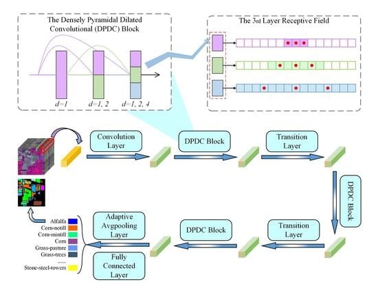
The receptive field is defined as the region dominated by each neuron in the model. In other words, the receptive field refers to the area where the pixels on the output feature of each layer are mapped on the original image in the convolutional neural network. The receptive field of the 3rd layer of the densely naive dilated convolutional block (Figure 3b) is depicted in Figure 4, and the size of convolutional kernel is $3\times 3$. Red dots represent the points to which the filter is applied, and colored backgrounds represent the receptive field covered by red dots.

Suppose that the input data is directly fed into these three blocks. The receptive field of the 3rd layer in the densely naive convolutional block: As shown in Figure 4a, firstly, the receptive field of $3\times 3$ (purple shaded area) corresponds to the skip connection between the input and the 3rd layer (see Figure 3a). Secondly, the receptive field of $5\times 5$ (green shaded area) corresponds to the skip connection between the 1st layer and the 3rd layer. Finally, the receptive field of $7\times 7$ (blue shaded area) corresponds to the skip connection between the 2nd layer and the 3rd layer. Furthermore, they correspond to a grid point in the output feature map (yellow shaded area).

The receptive field of the 3rd layer in the densely naive dilated convolutional block: As shown in Figure 4b, the receptive field of $3\times 3$ (purple shaded area) corresponds to the skip connection between the input and the 3rd layer (see Figure 3b), but it contains a large number of unrecognized areas, which leads to discontinuous hyperspectral information obtained. The skip connection from the 1st layer to the 3rd layer corresponds to a larger receptive field than the densely naive convolutional block, but there are still blind spots in the receptive field, which is caused by the unreasonable setting of the dilated factor.

The receptive field of the 3rd layer in the DPDC block: As shown in Figure 4c, compared with the receptive field of densely naive convolutioanl blocks, the skip connection from the 1st layer to the 3rd layer in the densely pyramidal dilated convolutional block (see Figure 3c) has a larger receptive field. Compared with densely naive dilated convolutional blocks, there are no blind spots in the receptive field corresponding to the skip connections from the 1st layer to the 3rd layer in the pyramidal dilated convolutional block. This is mainly benefited from our reasonable setting of the dilated factor and the design of the PDC layer. The PDC layer performs different convolutional operations on the feature maps from different skip connections. For instance, the 3rd PDC layer in Figure 3c performs $d=1$ and $d=2$ dilated convolutional operations on the feature maps from two different skip connections, respectively. In DenseNet, feature maps of all previous $k-1$ layers $[x_0,x_1,···,x_{k-1}]$ are used as the input of the $k_{th}$ layer:

$$X_k=R\left([x_0,x_1,···,x_{k-1}]\right)\otimes w_k,$$

(3)

where $R(·)$ refers to the composite operation of batch normalization and ReLU activation function. $[x_0,x_1,···,x_{k-1}]$ denotes the stacking of the feature maps ($x_0$: the input feature) on the channel from layer 0 to $k-1$, and the size of convolutional kernel ($w_k$) is $3\times 3$. The ${\otimes }_d$ with the dilated factor $d=2^{k-1}$ is used to represent the dilated convolution, and a variation of Equation (3) can be acquired by applying ${\otimes }_d$ to Densenet:

$$Y_k=R\left([x_0,x_1,···,x_{k-1}]\right){\otimes }_d{w}_k.$$

(4)

However, skip connections will cause blind spots in the receptive field, so that the feature information learned by the convolutional layer is not comprehensive. To overcome this problem, densely pyramidal dilated convolutional block is proposed and defined as follows:

$$H_k{\otimes }_{d_i}{W}_k=\sum _{i=1}^{k-1}{h}_i{\otimes }_{d_i}{w}_k^i,$$

(5)

where $H_k=[h_0,h_1,···,h_{k-1}]=R\left([x_0,x_1,···,x_{k-1}]\right)$ is the output of composite layer, $W_k$ refers to the set of convolutional kernels at the $k_{th}$ layer and $w_k^i$ denotes the convolutional kernel corresponding to the $i_{th}$ skip connection of the $k_{th}$ layer ($w_k^i$ is a subset of $W_k$). The continuity of spatial information is well preserved in the DPDC block (Figure 4c). In other words, blind spots problem in densely naive dilated convolutional block is effectively solved by choosing approprite dilated factors and increasing network width like a pyramid. The more comprehensive feature information of the PDC layer is obtained by pixel-level addition of feature maps of its internal sublayers. Furthermore, the dense connection mode is adopted between PDC layers, which can make more effective reuse of features.

3.4. PDCNet Model

Take PDCNet with three DPDC blocks as an example, its network structure is shown in Figure 5. $BN+ReLU+Convolution$ (hereinafter referred to as Conv) is used as our basic structure. Meanwhile, BN and ReLU operations are omitted in Figure 5. DenseNet model for HSI classification, DPDC block, receptive fields and dilated convolution were introduced in Section 3.1, Section 3.2 and Section 3.3. Although the size of the receptive field can be effectively increased by dilated convolution, feature information obtained is discontinuous due to the existence of blind spots. Therefore, while the dilated factors are effectively set in the DPDC block, network width gradually increases like a pyramid, which is conducive to eliminate blind spots, and acquire large-range and multi-scale feature information. Furthermore, to take advantage of the features of the previous layers, the dense connection pattern is introduced into PDCNet. High classification accuracy is achieved by combining dilated convolution and dense connection to extract more comprehensive and rich features. The Indian Pines dataset is applied as an example to feed into the PDCNet model proposed in this paper.

PDCNet is composed of three DPDC blocks and two transition layers. The transition layers are, respectively, embedded between the three DPDC blocks. The hyperspectral image is divided into cubes and fed into the proposed network. Firstly, the input features are sent to a convolution layer (the kernel size is $3\times 3$) for feature extraction, and then they are sent to the subsequent modules of the network. Each DPDC block is densely connected by different number of PDC layers, while the PDC layer $N_K$ is stacked by different sub-dilated convolutional layers $n_k^d$. The input features of the DPDC block will be allocated to the dilated convolutional layers in the PDC layer through skip connections. Secondly, a hybrid feature fusion mechanism is applied in PDCNet. As shown in Figure 3c, the DPDC block contains two feature fusion methods: pixel-by-pixel addition and channel stacking. The feature fusion method of channel stacking is adopted between different PDC layers, and the pixel-by-pixel addition is used within each PDC layer and channel stacking is applied between each PDC layers. The hybrid feature fusion mechanism can realize the reuse of all previous layers output features while integrating large-range and multi-scale feature maps. In order to flexibly change the number of channels and reduce the parameters, Conv (the kernel size is $1\times 1$) is applied in the transition layer. Finally, the classification results are obtained by an adaptive average pooling layer and a fully connected layer.

4. Experiments

4.1. Description of HSI Datasets

Indian Pines (IP): As a famous dataset for HSI classification, IP dataset was captured by the Airborne Visible/Infrared Imaging Spectrometer (AVIRIS) sensor over the remote sensing test site in the northwest area of the India, 1992. It is composed of 200 valid bands with spectral range from 0.4 to 2.5 $\mathsf{\mu }$m after discarding 20 water absorption bands. The image of IP has $145\times 145$ pixels with a spatial resolution of 20 mpp, and 16 vegetation classes are considered, e.g., alfalfa, oats, wheat, woods, etc. The ground-truth map, the false-color image and the corresponding color label are given in Figure 6.

Pavia University (UP): It was gathered by the Reflective Optices Spectrographic Imaging System (ROSIS) over the Pavia University in Italy, 2001. It is comprised of 103 effective bands with spectral range from 0.43 to 0.86 $\mathsf{\mu }$m after removing 12 noisy bands. The image of UP has $610\times 340$ pixels with spatial resolution of 1.3 mpp, and 9 feature categories are used, such as trees, gravel, bricks, etc. The ground-truth map, the false-color image and the corresponding color labels are revealed in Figure 7.

Salinas Valley (SV): SV dataset was obtained by the AVARIS senor over an agricultural region of SV, CV, USA, in 1998, and it is consisted of 204 effective bands with spectral range from 0.4 to 2.5 $\mathsf{\mu }$m after ignoring 20 bands of low signal to noise ratio (SNR). The image of SV has $512\times 217$ pixels with spatial resolution of 3.7 mpp, and 16 land cover classes are analyzed, e.g., fallow, stubble, celery, etc. The ground-truth map, the false-color image and the corresponding color labels are displayed in Figure 8.

4.2. Setting of Experimental Parameters

PyTorch deep learning framework is applied to a computer with 2.90 GHz Intel Core i5-10400F central processing unit (CPU) and 16 GB memory for experiments, and the average of five experimental results is taken as the final classification result. Three evaluation indicators are used to evaluate the performance of different networks: overall accuracy (OA), average accuracy (AA) and kappa coefficient (Kappa).

As shown in

Table 1. The number of samples in the IP dataset.

Number	Class	Train Samples	Test Samples	Total Samples
1	Alfalfa	7	39	46
2	Corn-notill	214	1214	1428
3	Corn-mintill	125	705	830
4	Corn	36	201	237
5	Grass-pasture	72	411	483
6	Grass-trees	110	620	730
7	Grass-pasture-mowed	4	24	28
8	Hay-windrowed	72	406	478
9	Oats	3	17	20
10	Soybean-notill	146	826	972
11	Soybean-mintill	368	2087	2455
12	Soybean-clean	89	504	593
13	Wheat	31	174	205
14	Woods	190	1075	1265
15	Buildings-grass-trees-drivers	58	328	386
16	Stone-steel-towers	14	79	93
	Sum	1539	8710	10,249

, 15% of the labeled samples in the IP dataset are used as the training set. Similarly, 5% and 2% of the label samples in the UP and SV datasets are used as the training set and the remaining labeled samples as the testing set (

Table 2. The number of samples in the UP dataset.

Number	Class	Train Samples	Test Samples	Total Samples
1	Asphalt	332	6299	6631
2	Meadows	932	17,717	18,649
3	Gravel	105	1994	2099
4	Trees	153	2911	3064
5	Painted metal sheets	67	1278	1345
6	Bare Soil	251	4778	5029
7	Bitumen	67	1263	1330
8	Self-Blocking Bricks	184	3498	3682
9	Shadows	47	900	947
	Sum	2138	40,638	42,776

and

Table 3. The number of samples in the SV dataset.

Number	Class	Train Samples	Test Samples	Total Samples
1	Brocoli_green_weeds_1	40	1969	2009
2	Brocoli_green_weeds_2	75	3651	3726
3	Fallow	40	1936	1976
4	Fallow_rough_plow	28	1366	1394
5	Fallow_smooth	54	2624	2678
6	Stubble	79	3880	3959
7	Celery	72	3507	3579
8	Grapes_untrained	225	11,046	11,271
9	Soil_vinyard_develop	124	6079	6203
10	Corn_senesced_green_weeds	66	3212	3278
11	Lettuce_romaine_4wk	21	1047	1068
12	Lettuce_romaine_5wk	39	1888	1927
13	Lettuce_romiane_6wk	18	898	916
14	Lettuce_romiane_7wk	21	1049	1070
15	Vinyard_untrained	145	7123	7268
16	Vinyard_vertical_trellis	36	1771	1807
	Sum	1083	53,046	54,129

). To better illustrate the robustness of the network, the performance of networks for comparison under different proportions of training samples will be shown in Section 5.

To verify the effectiveness of the method proposed in this paper, several network models are adopted for comparative experiments. The optimal parameters of SVM [9] are obtained by grid search algorithm, which is a traditional machine learning method. In addition, comparative experiments are also carried out on some methods based on deep learning: 3-D CNN [32], FDMFN [42], PresNet [41] and DenseNet [45]. A baseline network (BMNet) composed of three densely naive convolutional blocks and two transition layers, and a dilated convolutional network (DCNet) composed of three dense ordinary dilated convolutional blocks are proposed for comparison experiments in this paper.

The relevant hyper-parameters of the experiment are set as follows. The patch size of comparative experiments with other models is set to $11\times 11$, and the epoch and batch size is 100. The learning rate of 3D-CNN, FDMFN, DenseNet, and PDCNet are set to 0.001. The learning rate of PresNet is 0.1. We use AdaptiveMoment Estimation (Adam) optimizer to optimize the learning rate for 3D-CNN, FDMFN, DenseNet, and PDCNet. The Stochastic Gradient Descent (SGD) optimizer is used to optimize the learning rate of PresNet. We use Cosine Annealing LR scheduler in the comparative experiments.

4.3. Influence of Parameters

Growth Rate g: It is used to control output channels of the convolutional layer. In the DPDC block, the number of output channels of each PDC layer will increase by g. For instance, the final output channel number of a DPDC block with three PDC layers will increase by 3×g. By adjusting the parameter, the information flow in the network can be controlled flexibly. The growth rate g in PDCNet is set as 52 because it achieved the highest classification accuracy, as shown in

Table 4. OA (%) of PDCNet with different growth rate g in IP, UP, and SV datasets.

Datasets	40	46	52	58	64
IP	99.43 ± 0.28	99.39 ± 0.28	99.43 ± 0.20	99.39 ± 0.21	99.40 ± 0.22
UP	99.78 ± 0.02	99.80 ± 0.05	99.82 ± 0.06	99.81 ± 0.03	99.78 ± 0.07
SV	99.12 ± 0.25	99.09 ± 0.23	99.15 ± 0.13	99.05 ± 0.29	98.93 ± 0.24

.

PDC Layer: The influence of PDCNet with different numbers of PDC layers in each DPDC block on the overall accuracy is shown in

Table 5. OA (%) of PDCNet with different number of PDC layers in IP, UP, and SV datasets.

Datasets	2	3	4	5	6
IP	99.44 ± 0.20	99.43 ± 0.20	99.34 ± 0.23	99.45 ± 0.25	99.41 ± 0.24
UP	99.78 ± 0.01	99.82 ± 0.06	99.76 ± 0.03	99.77 ± 0.05	99.78 ± 0.04
SV	99.18 ± 0.17	99.15 ± 0.13	99.06 ± 0.25	99.02 ± 0.21	98.96 ± 0.15

. Note that here the number of DPDC blocks is fixed to 3. PDCNet with 5 PDC layers in each DPDC block has the highest OA on the IP dataset. However, PDCNet with 3 PDC layers and PDCNet with 5 PDC layers in each block have little difference in accuracy on the IP dataset, so we choose PDCNet with 3 PDC layers in each block. PDCNet, which contains 3 PDC layers in each DPDC block, has the highest OA on the UP dataset. PDCNet with 2 PDC layers in each DPDC block reached the highest OA on the SV dataset.

DPDC Block: The influence of PDCNet with different numbers of DPDC blocks on the overall accuracy is shown in

Table 6. OA (%) of PDCNet with different number of DPDC blocks in IP, UP, and SV datasets.

Datasets	1	2	3	4	5
IP	99.40 ± 0.19	99.47 ± 0.17	99.43 ± 0.20	99.44 ± 0.20	99.42 ± 0.21
UP	99.73 ± 0.09	99.81 ± 0.02	99.82 ± 0.06	99.78 ± 0.04	99.71 ± 0.06
SV	98.97 ± 0.22	99.14 ± 0.25	99.15 ± 0.13	98.95 ± 0.34	98.88 ± 0.28

. Note that here the number of PDC layers in each block is fixed to 3. PDCNet with 2 DPDC blocks has the highest OA on the IP dataset. PDCNet with 3 DPDC blocks has the highest OA on the UP dataset in Table 6. PDCNet with 3 DPDC blocks has the highest accuracy on the SV dataset.

From the perspective of accuracy, comparing Table 5 and Table 6, firstly, we choose PDCNet with 2 DPDC blocks and 3 PDC layers in each block as the optimal PDCNet in the IP dataset. Secondly, PDCNet with 3 DPDC blocks and 3 PDC layers in each block is considered the optimal PDCNet in the UP dataset. Finally, the PDCNet with 3 DPDC blocks and 2 PDC layers in each block has the highest accuracy in the SV dataset.

Patch Size: The impact of different patches on the overall accuracy of the network is shown in

Table 7. OA (%) of PDCNet with different patch size in IP, UP, and SV datasets.

Datasets	9	11	13	15	17
IP	99.36 ± 0.09	99.43 ± 0.20	99.50 ± 0.18	99.38 ± 0.10	99.46 ± 0.06
UP	99.74 ± 0.10	99.82 ± 0.06	99.80 ± 0.05	99.74 ± 0.05	99.71 ± 0.07
SV	98.53 ± 0.13	99.15 ± 0.13	99.29 ± 0.21	99.45 ± 0.15	99.67 ± 0.12

. The network proposed in this paper achieves good results under the different patch sizes. When the patch size is $11\times 11$, PDCNet has the highest accuracy on the UP dataset, and has good performance on other datasets. In addition, considering the impact of patch size on training time, the patch size of the PDCNet model is set to $11\times 11$.

4.4. Ablation Experiments

As shown in Figure 3, three different blocks are designed in the paper. BMNet: BMNet is constructed by stacking three densely naive convolutional blocks (Figure 3a) and two transition layers, where the dilated factor of each convolutional layer is 1, and then densely connecting three naive convolutional layers to form a densely dilated convolutional block. DCNet: Compared with BMNet, DCNet is constructed by stacking three densely dilated convolutional blocks (Figure 3b) and two transition layers, where the dilated factor ($d=2^{k-1}$) of each dilated convolutional layer increases in turn, which can obtain larger the receptive field. However, there are blind spots in the receptive field. PDCNet: In order to reasonably increase the receptive field without introducing blind spots in the receptive field, a PDC layer is proposed, which contains sub-dilated convolutional layers with different dilated factors (Figure 3c). The DPDC block is composed of three PDC layers, and their width increases as the depth increases like a pyramid. The basic structure of PDCNet consists of three DPDC blocks and two transition layers through cross-stacking. To illustrate the effectiveness of the network proposed in this paper, BMNet, DCNet and PDCNet are experimented under the same parameter settings (i.e., patch size, learning rate, growth rate, etc.).

The overall accuracy of BMNet, DCNet and PDCNet in different proportions of training samples is shown in Figure 9. Overall accuracy on IP dataset of training samples with different proportions is shown in Figure 9a. The overall accuracy of PDCNet is represented by the red line, which has the highest accuracy compared to other models. As depicted in Figure 9b, with the proportion of training samples increasing, the overall accuracy of three networks become more and more close, but on the whole, PDCNet still showed good performance. As shown in Figure 9c, the overall accuracy of PDCNet is much higher than that of other networks with 2% of training samples. The OA, AA and Kappa of BMNet, DCNet and PDCNet with the same hyper-parameter settings on the three datasets (IP, UP and SV datasets) are shown in Figure 10. As a whole, the proposed network has the highest classification performance.

4.5. Classification Results

4.5.1. Classification Results (IP Dataset)

The classification results of PDCNet framework and other comparison methods on IP datasets are shown in

Table 8. The classification results for the IP dataset based on 15% training samples. The best results are highlighted in bold font.

Class	SVM	3-D CNN	FDMFN	PresNet	DenseNet	PDCNet
1	66.15 ± 8.17	95.90 ± 1.26	88.21 ± 13.63	95.90 ± 3.08	96.92 ± 2.99	97.95 ± 1.92
2	81.55 ± 2.35	96.06 ± 0.79	97.50 ± 0.80	98.93 ± 0.35	99.32 ± 0.30	99.34 ± 0.32
3	76.83 ± 3.44	95.73 ± 1.26	97.44 ± 1.22	98.66 ± 0.98	99.57 ± 0.29	99.46 ± 0.57
4	70.33 ± 4.14	94.26 ± 4.66	96.64 ± 2.70	97.13 ± 3.28	97.43 ± 2.60	99.11 ± 1.34
5	92.55 ± 2.56	96.74 ± 1.16	98.59 ± 0.90	98.93 ± 0.91	99.32 ± 0.64	99.07 ± 1.03
6	96.75 ± 0.70	99.29 ± 0.28	99.52 ± 0.35	99.52 ± 0.51	99.55 ± 0.26	99.71 ± 0.26
7	80.83 ± 5.65	97.50 ± 3.33	93.33 ± 6.77	96.67 ± 4.86	97.50 ± 5.00	96.67 ± 3.12
8	98.33 ± 0.57	100.00 ± 0.0	100.00 ± 0.0	99.95 ± 0.10	100.00 ± 0.0	100.00 ± 0.0
9	63.53 ± 12.0	87.06 ± 5.76	91.76 ± 16.5	98.82 ± 2.35	95.29 ± 4.40	98.82 ± 2.35
10	77.74 ± 4.91	94.49 ± 1.94	97.57 ± 1.16	96.89 ± 1.37	98.13 ± 2.11	98.59 ± 1.39
11	84.32 ± 2.52	98.06 ± 0.69	99.32 ± 0.35	99.29 ± 0.54	98.76 ± 0.94	99.75 ± 0.19
12	80.83 ± 3.73	96.67 ± 1.24	97.75 ± 1.24	96.88 ± 1.16	99.05 ± 0.70	98.93 ± 0.69
13	96.32 ± 2.04	99.31 ± 0.67	99.77 ± 0.46	99.66 ± 0.46	100.00 ± 0.0	99.66 ± 0.46
14	94.42 ± 1.16	99.13 ± 0.62	99.65 ± 0.23	99.74 ± 0.27	99.70 ± 0.24	100.00 ± 0.0
15	67.52 ± 3.90	96.01 ± 4.80	96.50 ± 4.23	96.79 ± 3.01	99.64 ± 0.48	99.70 ± 0.46
16	92.66 ± 0.51	98.48 ± 1.86	99.24 ± 0.62	98.99 ± 0.51	97.72 ± 1.24	97.72 ± 0.95
OA (%)	84.54 ± 0.48	97.25 ± 0.09	98.47 ± 0.28	98.74 ± 0.26	99.12 ± 0.45	99.47 ± 0.17
AA (%)	82.54 ± 1.07	96.54 ± 0.40	97.05 ± 1.50	98.30 ± 0.50	98.62 ± 0.49	99.03 ± 0.31
Kappa (%)	82.39 ± 0.55	96.87 ± 0.10	98.25 ± 0.32	98.57 ± 0.30	99.00 ± 0.51	99.39 ± 0.20

. Correspondingly, Figure 11 shows classification maps of the model designed in this paper and other models, where Figure 11a,b are the false color image and the ground truth, respectively. Obviously, compared with other networks, the model designed in this paper has higher accuracy.

As shown in Table 8, the OA, AA and Kappa of the proposed network (PDCNet) are 99.47%, 99.03% and 99.39%, respectively. According to the classification results of Alfalfa (class 1), the accuracy of PDCNet reaches 97.95%, which is higher than that of other models. Compared with SVM, 3-D CNN, FDMFN, PresNet and DenseNet, the overall accuracy of the network proposed in this paper is increased by 14.93%, 2.22%, 1.00%, 0.73% and 0.35%, respectively. The average accuracy and Kappa coefficient are also improved to different degrees. As depicted in Figure 11, the classification accuracy of SVM is poor, and there are many noises and spots in classification map. Three-dimensional CNN has a poor ability to process edge information, which leads to edge classification errors in many categories, such as Corn-notill (class 2) and Soybean-notill (class 10) in the classification map. FDMFN, PresNet, DenseNet and PDCNet have better classification performance, but FDMFN has poor classification ability on Alfalfa and Corn-notill. Furthermore, PresNet cannot correctly classify the edges of Soybean-mintill (class 11) and Buildings-grass-trees-drivers (class 15). Furthermore, DenseNet achieves accuracy close to that of PDCNet, but internal noises of DenseNet is more than PDCNet. The problem can be avoided by setting the dilated factor in the dilated convolution reasonably.

While the PDC layer acquires a larger receptive field, it also ensures the continuity of spatial information, which can effectively reduce noise pollution in the receptive field. Therefore, compared with the classification results of other models, the classification map of PDCNet (Figure 11) has less noise and spots on the IP dataset.

4.5.2. Classification Results (UP Dataset)

The classification result of the proposed network and other comparison methods on the UP dataset are indicated in

Table 9. The classification results for the UP dataset based on 5% training samples. The best results are highlighted in bold font.

Class	SVM	3-D CNN	FDMFN	PresNet	DenseNet	PDCNet
1	92.98 ± 0.76	98.44 ± 1.00	99.38 ± 0.23	99.36 ± 0.14	99.77 ± 0.14	99.69 ± 0.31
2	97.33 ± 0.21	99.71 ± 0.15	99.90 ± 0.06	99.88 ± 0.08	99.96 ± 0.03	99.99 ± 0.01
3	76.97 ± 2.25	90.73 ± 2.91	95.74 ± 2.42	95.70 ± 2.67	98.35 ± 0.75	99.82 ± 0.13
4	87.15 ± 1.93	97.62 ± 0.89	98.83 ± 0.38	98.52 ± 0.59	98.91 ± 0.37	98.89 ± 0.52
5	99.31 ± 0.09	99.66 ± 0.36	99.92 ± 0.09	100.00 ± 0.0	99.84 ± 0.13	99.83 ± 0.10
6	77.14 ± 1.28	98.64 ± 1.74	98.86 ± 1.45	99.88 ± 0.15	99.99 ± 0.02	99.99 ± 0.01
7	58.04 ± 5.75	92.29 ± 3.89	98.15 ± 1.52	97.31 ± 2.00	99.76 ± 0.40	99.87 ± 0.15
8	85.25 ± 1.59	96.62 ± 1.81	99.11 ± 0.24	98.81 ± 0.86	99.78 ± 0.33	99.89 ± 0.19
9	99.84 ± 0.15	98.60 ± 0.62	99.64 ± 0.20	99.93 ± 0.13	99.02 ± 0.68	99.07 ± 0.74
OA (%)	90.67 ± 0.16	98.26 ± 0.79	99.28 ± 0.17	99.33 ± 0.09	99.73 ± 0.02	99.82 ± 0.06
AA (%)	86.00 ± 0.79	96.92 ± 1.22	98.84 ± 0.33	98.82 ± 0.24	99.49 ± 0.06	99.67 ± 0.08
Kappa (%)	87.26 ± 0.22	97.70 ± 1.04	99.05 ± 0.23	99.11 ± 0.12	99.65 ± 0.03	99.76 ± 0.07

. Correspondingly, Figure 12 indicates the classification maps of PDCNet model and other models, where Figure 12a,b are the false color image and the ground truth, respectively. In summary, the model suggested in this paper has the highest accuracy compared to other networks.

As shown in Table 9, the OA, AA and Kappa of the designed netwrok (PDCNet) reaches 99.82%, 98.67% and 99.76%, respectively. Compared with SVM, 3-D CNN, FDMFN, PresNet, DenseNet, the kappa coefficient of PDCNet is improved by 12.50%, 2.06%, 0.71%, 0.65% and 0.11%, respectively. The overall accuracy and average accuracy are also improved to different degrees. As depicted in Figure 12, there are many noises in the classification areas of Gravel (class 3), Bare Soil (class 6) and Bitumen (class 7) in the classification map of SVM. Relatively speaking, the methods based on deep learning can reduce noises on the classification map of UP dataset. However, 3-D CNN, FDMFN and PresNet still have unsatisfactory classification results on Gravel and Bitumen. Although DenseNet has better classification performance on Bitumen, there is still obvious wrong classification for Gravel. It is worth noting that PDCNet has good classification results on areas that are difficult to classify, such as Gravel, Bare Soil and Bitumen.

Compared with the single feature fusion method of DenseNet, the feature fusion mechanism that combines pixel-by-pixel addition and channel stacking applied in PDCNet is more effective, and a larger receptive field is captured by dilated convolution. The spectral–spatial features obtained by PDCNet are more abstract and comprehensive, which makes it possible to classify some areas that are more difficult to distinguish accurately.

4.5.3. Classification Results (SV Dataset)

The classification result of the network suggested in this paper (PDCNet) and other comparison methods on the SV dataset are shown in

Table 10. The classification results for the SV dataset based on 2% training samples. The best results are highlighted in bold font.

Class	SVM	3-D CNN	FDMFN	PresNet	DenseNet	PDCNet
1	98.32 ± 0.64	99.22 ± 0.90	99.57 ± 0.67	99.80 ± 0.22	84.33 ± 13.24	100.00 ± 0.0
2	99.67 ± 0.31	99.78 ± 0.18	99.96 ± 0.04	99.75 ± 0.48	99.98 ± 0.03	100.00 ± 0.0
3	96.55 ± 4.33	97.96 ± 2.10	99.73 ± 0.39	99.71 ± 0.24	99.12 ± 1.68	99.98 ± 0.04
4	99.18 ± 0.31	99.33 ± 0.50	99.50 ± 0.56	99.33 ± 0.29	99.41 ± 0.69	99.37 ± 0.55
5	98.31 ± 0.97	97.26 ± 0.93	99.71 ± 0.26	99.66 ± 0.22	99.64 ± 0.26	99.70 ± 0.35
6	99.61 ± 0.18	99.92 ± 0.11	99.99 ± 0.01	100.00 ± 0.0	100.00 ± 0.0	100.00 ± 0.0
7	99.44 ± 0.28	99.41 ± 0.25	99.94 ± 0.13	99.90 ± 0.10	99.97 ± 0.03	99.99 ± 0.01
8	86.92 ± 1.67	88.68 ± 1.25	93.05 ± 1.07	95.07 ± 0.31	96.15 ± 1.70	97.62 ± 0.62
9	99.04 ± 0.82	99.38 ± 0.46	100.00 ± 0.0	99.89 ± 0.13	99.69 ± 0.55	100.00 ± 0.0
10	94.24 ± 0.73	96.37 ± 1.72	98.64 ± 0.96	98.85 ± 0.92	99.59 ± 0.41	99.68 ± 0.36
11	94.01 ± 3.98	97.25 ± 1.77	99.69 ± 0.35	98.93 ± 1.06	99.64 ± 0.36	99.90 ± 0.15
12	99.51 ± 0.41	99.59 ± 0.35	99.99 ± 0.02	99.99 ± 0.02	100.00 ± 0.0	100.00 ± 0.0
13	98.37 ± 0.58	99.35 ± 0.46	99.93 ± 0.09	100.00 ± 0.0	100.00 ± 0.0	100.00 ± 0.0
14	91.08 ± 2.20	97.16 ± 1.65	99.81 ± 0.13	99.92 ± 0.11	99.56 ± 0.74	99.96 ± 0.05
15	61.00 ± 2.57	77.19 ± 3.89	94.61 ± 1.09	95.58 ± 1.22	97.42 ± 1.81	98.03 ± 0.90
16	98.05 ± 0.98	97.38 ± 1.02	98.45 ± 0.70	99.00 ± 0.64	99.67 ± 0.28	99.74 ± 0.23
OA (%)	90.66 ± 0.50	93.75 ± 0.78	97.62 ± 0.19	98.16 ± 0.15	98.12 ± 0.78	99.18 ± 0.17
AA (%)	94.58 ± 0.62	96.58 ± 0.41	98.91 ± 0.05	99.09 ± 0.13	98.39 ± 1.04	99.62 ± 0.07
Kappa (%)	89.59 ± 0.55	93.03 ± 0.87	97.35 ± 0.21	97.96 ± 0.17	97.90 ± 0.87	99.08 ± 0.19

. Correspondingly, Figure 13 shows the classification maps of PDCNet and other models, where Figure 13a,b are the false color image and the ground truth, respectively. In short, the proposed model has higher accuracy compared to other networks on the SV dataset.

As shown in Table 10, the OA, AA and Kappa of the network proposed in this paper (PDCNet) obtains the classification results of 99.18%, 99.62% and 99.08%, respectively. Compared with SVM, 3-D CNN, FDMFN, PresNet, DenseNet, overall accuracy of PDCNet is improved by 8.52%, 5.43%, 1.56%, 1.02% and 1.06%, respectively. The overall accuracy and the average accuracy are also improved to different degrees. As depicted in Figure 13, SVM cannot classify Grapes_untrained (class 8) and Vinyard_untrained (class 15) well, and there is serious noise pollution in the classification area of these categories. Although 3-D CNN alleviates the problem of noise pollution to a certrain extent, it is more sensitive to edge information, such as Soil_vinyard_develop (class 9), Lettuce_romiane_7wk (class 14) and Corn_senesced_green_weeds (class 10). In addition, for Grapes_untrained and Vinyard_untrained, PDCNet has less pollution and higher classification results than FDMFN, PresNet and DenseNet.

The higher classification results are mainly attributed to the combination of two ideas in PDCNet. Firstly, the blind spot problem in the receptive field is solved by setting the dilated factor reasonably and increasing the network width like a pyramid, which makes the classification map have less noise and spots. Secondly, the feature fusion method of the hybrid mode is adopted to obtain richer and comprehensive feature information. Furthermore, a larger receptive field is acquired through dilated convolution, which allows the edge features of each category to be better distinguished.

From the perspective of experimental results, compared with some traditional classification methods, the PDCNet proposed in this paper shows the best classification results on the three datasets. Firstly, from the classification accuracy of the three datasets, PDCNet obtained the highest classification accuracy. Secondly, the classification map of PDCNet on the three datasets suffers the least pollution, and it contains the least noise and spots. From the point of view of the network structure, we have introduced dilated convolution and short connections in the DPDC block, while obtaining a larger receptive field, it also eliminates the problem of blind spots caused by dilated convolution, which allows PDCNet to obtain more continuous and comprehensive spatial information.

4.6. Comparison with Other Segmentation Method

In this section, we use the PDCNet model structure shown in Figure 5 to conduct a comparative experiment with another hyperspectral image segmentation method (DeepLab v3+) [49] on the UP and KSC datasets. The corresponding classification results are shown in

Table 11. The classification results of PDCNet and DeepLab v3+ on the KSC and UP datasets based on 5% of the training samples.

Class	KSC (5%)		UP (5%)
	DeepLab v3+	PDCNet	DeepLab v3+	PDCNet
1	98.89	100.0	99.19	99.69
2	100.0	95.84	99.48	99.99
3	97.98	97.53	99.30	99.82
4	99.13	88.79	97.53	98.89
5	96.20	90.20	99.92	99.83
6	100.0	98.06	99.79	99.99
7	100.0	92.20	98.90	99.87
8	91.42	98.98	96.91	99.89
9	100.0	100.0	99.78	99.07
10	99.47	99.53	/	/
11	98.74	99.65	/	/
12	97.88	99.54	/	/
13	100.0	100.0	/	/
OA (%)	98.47	98.40	99.10	99.82
AA (%)	98.44	96.95	98.98	99.67
Kappa (%)	98.29	98.22	98.81	99.76

. We randomly select 5% of the labeled training samples in the UP and KSC datasets.

As shown in Table 11, the network proposed in this paper and DeepLab v3+ achieved similar OA and Kappa on the KSC dataset. However, AA of PDCNet is lower than that of DeepLab v3+. It is worth noting that the accuracy of PDCNet on the UP dataset is higher than DeepLab v3+. Among them, the OA, AA and Kappa of PDCNet are 0.72%, 0.31% and 0.95% higher than those of DeepLab v3+, respectively. Overall, PDCNet has achieved similar OA and Kappa to DeepLab v3+ on the KSC dataset. The OA, AA and Kappa of PDCNet on the UP dataset are all higher than DeepLab v3+.

5. Discussion

5.1. Influence of Training Samples

Different proportions of training samples on IP, UP and SV datasets are adopted to measure the performance of different networks. The overall accuracy of SVM, 3D CNN, FDMFN, PresNet, DenseNet and PDCNet are shown in

Table 12. OA(%) of different methods with different proportions of training samples. The best results are highlighted in bold font.

Dataset	Training Samples	SVM	3-D CNN	FDMFN	PresNet	DenseNet	PDCNet
IP	12.0%	83.19 ± 0.60	95.98 ± 0.23	97.60 ± 0.35	98.38 ± 0.27	98.91 ± 0.27	99.17 ± 0.19
	13.0%	83.88 ± 0.58	96.63 ± 0.09	98.04 ± 0.33	98.56 ± 0.31	98.95 ± 0.28	99.22 ± 0.34
	14.0%	84.27 ± 0.59	96.95 ± 0.09	98.30 ± 0.36	98.58 ± 0.45	99.03 ± 0.33	99.34 ± 0.20
	15.0%	84.54 ± 0.48	97.25 ± 0.09	98.47 ± 0.28	98.74 ± 0.26	99.12 ± 0.45	99.43 ± 0.20
	16.0%	84.82 ± 0.65	97.76 ± 0.26	98.70 ± 0.34	99.05 ± 0.24	99.36 ± 0.20	99.50 ± 0.19
UP	4.00%	90.32 ± 0.16	96.84 ± 1.86	98.82 ± 0.24	98.80 ± 0.26	99.57 ± 0.07	99.60 ± 0.06
	5.00%	90.67 ± 0.16	98.26 ± 0.79	99.28 ± 0.17	99.33 ± 0.09	99.73 ± 0.02	99.82 ± 0.06
	6.00%	90.85 ± 0.16	98.58 ± 0.65	99.54 ± 0.12	99.49 ± 0.21	99.75 ± 0.07	99.85 ± 0.03
	7.00%	90.95 ± 0.14	98.75 ± 0.43	99.61 ± 0.08	99.62 ± 0.19	99.79 ± 0.03	99.89 ± 0.04
	8.00%	91.05 ± 0.11	98.79 ± 0.57	99.65 ± 0.10	99.65 ± 0.15	99.77 ± 0.16	99.88 ± 0.05
SV	2.00%	90.66 ± 0.50	93.75 ± 0.78	97.62 ± 0.19	98.16 ± 0.15	98.12 ± 0.78	99.15 ± 0.13
	3.00%	91.35 ± 0.23	94.46 ± 0.50	97.98 ± 0.49	98.09 ± 0.32	97.98 ± 0.90	99.18 ± 0.33
	4.00%	91.90 ± 0.22	95.91 ± 0.40	98.98 ± 0.14	99.42 ± 0.12	99.48 ± 0.20	99.75 ± 0.07
	5.00%	92.12 ± 0.18	96.59 ± 0.50	99.27 ± 0.15	99.48 ± 0.18	99.64 ± 0.10	99.86 ± 0.07
	6.00%	92.36 ± 0.14	96.71 ± 0.27	99.36 ± 0.13	99.57 ± 0.19	99.66 ± 0.15	99.88 ± 0.05

. Note that here PDCNet with 3 DPDC blocks (3 PDC layers in each block) is used for comparison. On the IP dataset, the netwrok suggested in this paper is 0.79%, 0.66%, 0.69%, 0.45% higher than PresNet, and 0.26%, 0.27%, 0.31%, 0.31%, 0.14% higher than DenseNet. The overall accuracy of PDCNet is also improved in UP and SV datasets. The designed network shows great overall accuracy under different proportion of training samples.

5.2. Analysis of Running Time and Number of Network Parameters

Table 13. Comparison of networks parameters and running time.

Dataset	Method	Training Time (s)	Testing Time (s)	Total Params (M)
IP	SVM	16.562	5.270	/
	3-D CNN	77.328	4.313	0.101
	FDMFN	45.623	2.177	0.139
	PresNet	77.152	3.975	1.126
	DenseNet	108.55	5.229	4.749
	PDCNet	180.27	3.578	1.020
UP	SVM	12.294	12.575	/
	3-D CNN	63.365	22.895	0.050
	FDMFN	53.930	15.485	0.137
	PresNet	96.108	34.141	1.110
	DenseNet	138.71	47.872	4.651
	PDCNet	234.46	29.790	0.927
SV	SVM	6.967	9.888	/
	3-D CNN	53.659	22.261	0.103
	FDMFN	32.264	11.695	0.139
	PresNet	54.216	21.372	1.127
	DenseNet	75.681	28.788	4.753
	PDCNet	125.25	19.043	1.024

shows the running time and parameters of different networks on IP, UP and SV datasets. Note that here PDCNet with three DPDC blocks and three PDC layers in each block is used for comparison. Since the PDC layer in PDCNet could contain several sub-dilated convolutional layers, the training time of the network designed in this paper is longer than that of other networks. In addition, the parameters of the suggested network are more than those of 3D CNN and FDMFN. However, the proposed network has fewer parameters than DenseNet and PresNet.

6. Conclusions

In this paper, we propose a densely connected pyramidal dilated convolutional neural network for hyperspectral image classification, which can capture more comprehensive spatial information. Firstly, the PDC layer is composed of different numbers of dilated convolutions with different dilated factors to obtain receptive fields of multiple scales. Secondly, in order to eliminate blind spots in the receptive field, we densely connect different numbers of PDC layers to form a DPDC block. It can be seen from the classification result maps on the three datasets that the classification map of PDCNet suffers the least pollution and contains the least noise and spots, which is mainly due to the design of the DPDC block. Finally, a hybrid feature fusion mechanism of pixel-by-pixel addition and channel stacking is applied in PDCNet to improve the discriminative power of features. This is another reason for our good classification accuracy. In addition, the experimental results on three datasets show that our method can obtain good classification performance compared with other popular models.

In future work, since we have increased the width of the network, the training time of PDCNet is relatively long. Therefore, some methods to reduce computing cost will be considered and applied to the network in this paper. In addition, in order to further obtain more abstract spectral–spatial features, some new methods will be considered, such as channel shuffling technology and the utilization of more frequency domain information in pooling layer.

References

- Shabbir, S.; Ahmad, M. Hyperspectral image classification–traditional to deep models: A survey for future prospects. arXiv 2021, arXiv:2101.06116. [Google Scholar]
- Han, Y.; Li, J.; Zhang, Y.; Hong, Z.; Wang, J. Sea ice detection based on an improved similarity measurement method using hyperspectral data. Sensors 2017, 17, 1124. [Google Scholar] [CrossRef] [Green Version]
- Stuart, M.B.; McGonigle, A.J.; Willmott, J.R. Hyperspectral imaging in environmental monitoring: A review of recent developments and technological advances in compact field deployable systems. Sensors 2019, 19, 3071. [Google Scholar] [CrossRef] [Green Version]
- Garzon-Lopez, C.X.; Lasso, E. Species classification in a tropical alpine ecosystem using UAV-Borne RGB and hyperspectral imagery. Drones 2020, 4, 69. [Google Scholar] [CrossRef]
- Borana, S.; Yadav, S.; Parihar, S. Hyperspectral data analysis for arid vegetation species: Smart & sustainable growth. In Proceedings of the 2019 International Conference on Computing, Communication, and Intelligent Systems (ICCCIS), Greater Noida, India, 18–19 October 2019; pp. 495–500. [Google Scholar]
- Zhu, M.; Jiao, L.; Liu, F.; Yang, S.; Wang, J. Residual spectral–spatial attention network for hyperspectral image classification. IEEE Trans. Geosci. Remote Sens. 2020, 59, 449–462. [Google Scholar] [CrossRef]
- Meng, Z.; Jiao, L.; Liang, M.; Zhao, F. A lightweight spectral-spatial convolution module for hyperspectral image classification. IEEE Geosci. Remote Sens. Lett. 2021, 1–5. [Google Scholar] [CrossRef]
- Signoroni, A.; Savardi, M.; Baronio, A.; Benini, S. Deep learning meets hyperspectral image analysis: A multidisciplinary review. J. Imaging 2019, 5, 52. [Google Scholar] [CrossRef] [Green Version]
- Melgani, F.; Bruzzone, L. Classification of hyperspectral remote sensing images with support vector machines. IEEE Trans. Geosci. Remote Sens. 2004, 42, 1778–1790. [Google Scholar] [CrossRef] [Green Version]
- Okwuashi, O.; Ndehedehe, C.E. Deep support vector machine for hyperspectral image classification. Pattern Recognit. 2020, 103, 107298. [Google Scholar] [CrossRef]
- Sabat-Tomala, A.; Raczko, E.; Zagajewski, B. Comparison of support vector machine and random forest algorithms for invasive and expansive species classification using airborne hyperspectral data. Remote Sens. 2020, 12, 516. [Google Scholar] [CrossRef] [Green Version]
- Wang, A.; Wang, Y.; Chen, Y. Hyperspectral image classification based on convolutional neural network and random forest. Remote Sens. Lett. 2019, 10, 1086–1094. [Google Scholar] [CrossRef]
- Zhang, Y.; Cao, G.; Li, X.; Wang, B. Cascaded random forest for hyperspectral image classification. IEEE J. Sel. Top. Appl. Earth Obs. Remote Sens. 2018, 11, 1082–1094. [Google Scholar] [CrossRef]
- Cariou, C.; Le Moan, S.; Chehdi, K. Improving k-nearest neighbor approaches for density-based pixel clustering in hyperspectral remote sensing images. Remote Sens. 2020, 12, 3745. [Google Scholar] [CrossRef]
- Tu, B.; Wang, J.; Kang, X.; Zhang, G.; Ou, X.; Guo, L. KNN-based representation of superpixels for hyperspectral image classification. IEEE J. Sel. Top. Appl. Earth Obs. Remote Sens. 2018, 11, 4032–4047. [Google Scholar] [CrossRef]
- Su, H.; Yu, Y.; Wu, Z.; Du, Q. Random subspace-based k-nearest class collaborative representation for hyperspectral image classification. IEEE Trans. Geosci. Remote Sens. 2020, 59, 6840–6853. [Google Scholar] [CrossRef]
- Haut, J.M.; Paoletti, M.E.; Plaza, J.; Li, J.; Plaza, A. Active learning with convolutional neural networks for hyperspectral image classification using a new bayesian approach. IEEE Trans. Geosci. Remote Sens. 2018, 56, 6440–6461. [Google Scholar] [CrossRef]
- Zhan, Y.; Hu, D.; Wang, Y.; Yu, X. Semisupervised hyperspectral image classification based on generative adversarial networks. IEEE Geosci. Remote Sens. Lett. 2017, 15, 212–216. [Google Scholar] [CrossRef]
- Zhu, L.; Chen, Y.; Ghamisi, P.; Benediktsson, J.A. Generative adversarial networks for hyperspectral image classification. IEEE Trans. Geosci. Remote Sens. 2018, 56, 5046–5063. [Google Scholar] [CrossRef]
- Wang, H.; Tao, C.; Qi, J.; Li, H.; Tang, Y. Semi-supervised variational generative adversarial networks for hyperspectral image classification. In Proceedings of the 2019 IEEE International Geoscience and Remote Sensing Symposium (IGARSS), Yokohama, Japan, 28 July–2 August 2019; pp. 9792–9794. [Google Scholar]
- Mou, L.; Ghamisi, P.; Zhu, X.X. Deep recurrent neural networks for hyperspectral image classification. IEEE Trans. Geosci. Remote Sens. 2017, 55, 3639–3655. [Google Scholar] [CrossRef] [Green Version]
- Zhang, X.; Sun, Y.; Jiang, K.; Li, C.; Jiao, L.; Zhou, H. Spatial sequential recurrent neural network for hyperspectral image classification. IEEE J. Sel. Top. Appl. Earth Obs. Remote Sens. 2018, 11, 4141–4155. [Google Scholar] [CrossRef] [Green Version]
- Hang, R.; Liu, Q.; Hong, D.; Ghamisi, P. Cascaded recurrent neural networks for hyperspectral image classification. IEEE Trans. Geosci. Remote Sens. 2019, 57, 5384–5394. [Google Scholar] [CrossRef] [Green Version]
- Jiao, L.; Liang, M.; Chen, H.; Yang, S.; Liu, H.; Cao, X. Deep fully convolutional network-based spatial distribution prediction for hyperspectral image classification. IEEE Trans. Geosci. Remote Sens. 2017, 55, 5585–5599. [Google Scholar] [CrossRef]
- Li, J.; Zhao, X.; Li, Y.; Du, Q.; Xi, B.; Hu, J. Classification of hyperspectral imagery using a new fully convolutional neural network. IEEE Geosci. Remote Sens. Lett. 2018, 15, 292–296. [Google Scholar] [CrossRef]
- Zou, L.; Zhu, X.; Wu, C.; Liu, Y.; Qu, L. Spectral–spatial exploration for hyperspectral image classification via the fusion of fully convolutional networks. IEEE J. Sel. Top. Appl. Earth Obs. Remote Sens. 2020, 13, 659–674. [Google Scholar] [CrossRef]
- Xu, H.; Yao, W.; Cheng, L.; Li, B. Multiple spectral resolution 3D convolutional neural network for hyperspectral image classification. Remote Sens. 2021, 13, 1248. [Google Scholar] [CrossRef]
- Qing, Y.; Liu, W. Hyperspectral image classification based on multi-Scale residual network with attention mechanism. Remote Sens. 2021, 13, 335. [Google Scholar] [CrossRef]
- Rao, M.; Tang, P.; Zhang, Z. A developed siamese CNN with 3D adaptive spatial-spectral pyramid pooling for hyperspectral image classification. Remote Sens. 2020, 12, 1964. [Google Scholar] [CrossRef]
- Miclea, A.V.; Terebes, R.; Meza, S. One dimensional convolutional neural networks and local binary patterns for hyperspectral image classification. In Proceedings of the 2020 IEEE International Conference on Automation, Quality and Testing, Robotics (AQTR), Cluj-Napoca, Romania, 21–23 May 2020; pp. 1–6. [Google Scholar]
- Cao, X.; Yao, J.; Xu, Z.; Meng, D. Hyperspectral image classification with convolutional neural network and active learning. IEEE Trans. Geosci. Remote Sens. 2020, 58, 4604–4616. [Google Scholar] [CrossRef]
- Li, Y.; Zhang, H.; Shen, Q. Spectral–spatial classification of hyperspectral imagery with 3D convolutional neural network. Remote Sens. 2017, 9, 67. [Google Scholar] [CrossRef] [Green Version]
- Woo, S.; Park, J.; Lee, J.Y.; Kweon, I.S. CBAM: Convolutional block attention module. In Proceedings of the European Conference on Computer Vision (ECCV), Munich, Germany, 8–14 September 2018; pp. 3–19. [Google Scholar]
- Ma, W.; Yang, Q.; Wu, Y.; Zhao, W.; Zhang, X. Double-branch multi-attention mechanism network for hyperspectral image classification. Remote Sens. 2019, 11, 1307. [Google Scholar] [CrossRef] [Green Version]
- Li, R.; Zheng, S.; Duan, C.; Yang, Y.; Wang, X. Classification of hyperspectral image based on double-branch dual-attention mechanism network. Remote Sens. 2020, 12, 582. [Google Scholar] [CrossRef] [Green Version]
- He, K.; Zhang, X.; Ren, S.; Sun, J. Deep residual learning for image recognition. In Proceedings of the IEEE Conference on Computer Vision and Pattern Recognition (CVPR), Las Vegas, NV, USA, 27–30 June 2016; pp. 770–778. [Google Scholar]
- Zhong, Z.; Li, J.; Ma, L.; Jiang, H.; Zhao, H. Deep residual networks for hyperspectral image classification. In Proceedings of the 2017 IEEE International Geoscience and Remote Sensing Symposium (IGARSS), Fort Worth, TX, USA, 23–28 July 2017; pp. 1824–1827. [Google Scholar]
- Zhong, Z.; Li, J.; Luo, Z.; Chapman, M. Spectral–spatial residual network for hyperspectral image classification: A 3-D deep learning framework. IEEE Trans. Geosci. Remote Sens. 2017, 56, 847–858. [Google Scholar] [CrossRef]
- Meng, Z.; Li, L.; Tang, X.; Feng, Z.; Jiao, L.; Liang, M. Multipath residual network for spectral-spatial hyperspectral image classification. Remote Sens. 2019, 11, 1896. [Google Scholar] [CrossRef] [Green Version]
- Han, D.; Kim, J.; Kim, J. Deep pyramidal residual networks. In Proceedings of the IEEE Conference on Computer Vision and Pattern Recognition (CVPR), Honolulu, HI, USA, 21–26 July 2017; pp. 5927–5935. [Google Scholar]
- Paoletti, M.E.; Haut, J.M.; Fernandez-Beltran, R.; Plaza, J.; Plaza, A.J.; Pla, F. Deep pyramidal residual networks for spectral–spatial hyperspectral image classification. IEEE Trans. Geosci. Remote Sens. 2018, 57, 740–754. [Google Scholar] [CrossRef]
- Meng, Z.; Li, L.; Jiao, L.; Feng, Z.; Tang, X.; Liang, M. Fully dense multiscale fusion network for hyperspectral image classification. Remote Sens. 2019, 11, 2718. [Google Scholar] [CrossRef] [Green Version]
- Huang, G.; Liu, Z.; Van Der Maaten, L.; Weinberger, K.Q. Densely connected convolutional networks. In Proceedings of the IEEE Conference on Computer Vision and Pattern Recognition (CVPR), Honolulu, HI, USA, 21–26 July 2017; pp. 4700–4708. [Google Scholar]
- Meng, Z.; Jiao, L.; Liang, M.; Zhao, F. Hyperspectral image classification with mixed link networks. IEEE J. Sel. Top. Appl. Earth Obs. Remote Sens. 2021, 14, 2494–2507. [Google Scholar] [CrossRef]
- Paoletti, M.E.; Haut, J.M.; Plaza, J.; Plaza, A. Deep&dense convolutional neural network for hyperspectral image classification. Remote Sens. 2018, 10, 1454. [Google Scholar]
- Nalepa, J.; Antoniak, M.; Myller, M.; Lorenzo, P.R.; Marcinkiewicz, M. Towards resource-frugal deep convolutional neural networks for hyperspectral image segmentation. Microprocess. Microsyst. 2020, 73, 102994. [Google Scholar] [CrossRef]
- Fu, P.; Sun, X.; Sun, Q. Hyperspectral image segmentation via frequency-based similarity for mixed noise estimation. Remote Sens. 2017, 9, 1237. [Google Scholar] [CrossRef] [Green Version]
- Sun, H.; Zheng, X.; Lu, X. A supervised segmentation network for hyperspectral image classification. IEEE Trans. Image Process 2021, 30, 2810–2825. [Google Scholar] [CrossRef]
- Si, Y.; Gong, D.; Guo, Y.; Zhu, X.; Huang, Q.; Evans, J.; He, S.; Sun, Y. An Advanced Spectral–Spatial Classification Framework for Hyperspectral Imagery Based on DeepLab v3+. Appl. Sci. 2021, 11, 5703. [Google Scholar] [CrossRef]
- Takahashi, N.; Mitsufuji, Y. Densely connected multidilated convolutional networks for dense prediction tasks. arXiv 2020, arXiv:2011.11844. [Google Scholar]
- Meng, Z.; Zhao, F.; Liang, M.; Xie, W. Deep Residual Involution Network for Hyperspectral Image Classification. Remote Sens. 2021, 13, 3055. [Google Scholar] [CrossRef]
- Shi, H.; Cao, G.; Ge, Z.; Zhang, Y.; Fu, P. Double-Branch Network with Pyramidal Convolution and Iterative Attention for Hyperspectral Image Classification. Remote Sens. 2021, 13, 1403. [Google Scholar] [CrossRef]
- Gong, H.; Li, Q.; Li, C.; Dai, H.; He, Z.; Wang, W.; Li, H.; Han, F.; Tuniyazi, A.; Mu, T. Multiscale Information Fusion for Hyperspectral Image Classification Based on Hybrid 2D-3D CNN. Remote Sens. 2021, 13, 2268. [Google Scholar] [CrossRef]
- Li, C.; Qiu, Z.; Cao, X.; Chen, Z.; Gao, H.; Hua, Z. Hybrid Dilated Convolution with Multi-Scale Residual Fusion Network for Hyperspectral Image Classification. Micromachines 2021, 12, 545. [Google Scholar] [CrossRef] [PubMed]
- Gao, H.; Chen, Z.; Li, C. Hierarchical Shrinkage Multi-Scale Network for Hyperspectral Image Classification with Hierarchical Feature Fusion. IEEE J. Sel. Top. Appl. Earth Obs. Remote Sens. 2021, 14, 5760–5772. [Google Scholar] [CrossRef]
- Simonyan, K.; Zisserman, A. Very deep convolutional networks for large-scale image recognition. arXiv 2014, arXiv:1409.1556. [Google Scholar]
Figure 1.
The ways of two different convolutions. (a) Naive convolution. (b) Dilated convolution.
Figure 2.
Densely connected convolutional block of DenseNet.
Figure 3.
The structures of three different blocks. (a) Densely naive convolutional block. (b) Densely naive dilated convolutional block. (c) Densely pyramidal dilated convolutional block.
Figure 4.
The receiving fields of the 3rd layer in the different convolutional block (in the case of one-dimension). (a) The receptive field (densely naive convolutional block). (b) The receptive field (densely naive dilated convolutional block). (c) The receptive field (densely pyramidal dilated convolutional block).
Figure 5.
The framework of PDCNet.
Figure 6.
The Indian Pines Dataset. (a) The false-color image. (b) The ground-truth map. (c) The corresponding color labels.
Figure 7.
The Pavia University dataset. (a) The false-color image. (b) The ground-truth map. (c) The corresponding color labels.
Figure 8.
The Salinas Valley dataset. (a) The false-color image. (b) The ground-truth map. (c) The corresponding color labels.
Figure 9.
OA of different training samples with three datasets on BMNet, DCNet and PDCNet. (a) OA on IP dataset. (b) OA on UP dataset. (c) OA on SV dataset.
Figure 10.
Performance of BMNet, DCNet and PDCNet on different HSI datasets. (a) Metrics on IP dataset. (b) Metrics on UP dataset. (c) Metrics on SV dataset.
Figure 11.
Classification performance of different network models over IP dataset. (a) False-color image. (b) Ground truth. (c) SVM. (d) 3-D CNN. (e) FDMFN. (f) DenseNet. (g) PresNet. (h) PDCNet.
Figure 12.
Classification performance of different network models over UP dataset. (a) False-color image. (b) Ground truth. (c) SVM. (d) 3-D CNN. (e) FDMFN. (f) DenseNet. (g) PresNet. (h) PDCNet.
Figure 13.
Classification performance of different network models over SV dataset. (a) False-color image. (b) Ground truth. (c) SVM. (d) 3-D CNN. (e) FDMFN. (f) DenseNet. (g) PresNet. (h) PDCNet.