
RGB Indices and Canopy Height Modelling for Mapping Tidal Marsh Biomass from a Small Unmanned Aerial System


1
Department of Geography, University of South Carolina, Columbia, SC 29208, USA
2
Belle Baruch Institute for Marine & Coastal Sciences, University of South Carolina, Columbia, SC 29208, USA
*
Author to whom correspondence should be addressed.
Remote Sens. 2021, 13(17), 3406; https://0-doi-org.brum.beds.ac.uk/10.3390/rs13173406
Submission received: 26 July 2021
/
Revised: 25 August 2021
/
Accepted: 26 August 2021
/
Published: 27 August 2021
(This article belongs to the Special Issue Big Earth Data and Remote Sensing in Coastal Environments)
Abstract
:Coastal tidal marshes are essential ecosystems for both economic and ecological reasons. They necessitate regular monitoring as the effects of climate change begin to be manifested in changes to marsh vegetation healthiness. Small unmanned aerial systems (sUAS) build upon previously established remote sensing techniques to monitor a variety of vegetation health metrics, including biomass, with improved flexibility and affordability of data acquisition. The goal of this study was to establish the use of RGB-based vegetation indices for mapping and monitoring tidal marsh vegetation (i.e., Spartina alterniflora) biomass. Flights over tidal marsh study sites were conducted using a multi-spectral camera on a quadcopter sUAS near vegetation peak growth. A number of RGB indices were extracted to build a non-linear biomass model. A canopy height model was developed using sUAS-derived digital surface models and LiDAR-derived digital terrain models to assess its contribution to the biomass model. Results found that the distance-based RGB indices outperformed the regular radio-based indices in coastal marshes. The best-performing biomass models used the triangular greenness index (TGI; R2 = 0.39) and excess green index (ExG; R2 = 0.376). The estimated biomass revealed high biomass predictions at the fertilized marsh plots in the Long-Term Research in Environmental Biology (LTREB) project at the study site. The sUAS-extracted canopy height was not statistically significant in biomass estimation but showed similar explanatory power to other studies. Due to the lack of biomass samples in the inner estuary, the proposed biomass model in low marsh does not perform as well as the high marsh that is close to shore and accessible for biomass sampling. Further research of low marsh is required to better understand the best conditions for S. alterniflora biomass estimation using sUAS as an on-demand, personal remote sensing tool.
1. Introduction
Coastal tidal marshes are dynamic environments that serve a variety of ecological and economic functions in coastal regions. Beyond providing nurseries for many important aquatic species and beautiful backdrops for tourists, they also are known for carbon sequestration and water runoff filtration [1,2,3]. Despite their utility, tidal marshes face various challenges, including sea-level rise and erosion. Climate change threatens the natural order of tidal marshes by strengthening various environmental stressors that are predicted to impact vegetation biomass and other biophysical characteristics, eventually leading to loss of vegetation [4,5]. The benefits of and future challenges for coastal tidal marshes have led many community stakeholders to recognize the importance of regular assessment and monitoring of these environments [6] (p. 34). Successful marsh health monitoring requires the use of several metrics, including vegetation height, biomass, and density [7,8,9,10]. The complex nature of the tidal marsh environment presents challenges for frequently and efficiently gathering these metrics using in situ methods [11]. Remote sensing techniques have long provided non-intrusive methods for obtaining useful biophysical measurements [12].
The use of satellite imagery has been particularly successful in estimating one important biophysical measurement, marsh vegetation biomass. The use of remote sensing for estimating biomass of Spartina alterniflora (hereafter S. alterniflora), a common tidal marsh cordgrass, was introduced in 1983 [13]. The study simulated bands 3, 4, and 5 of a Landsat TM imagery by collecting spectral radiance data and determining the relationships between vegetation indices and collected biomass measurements, and found that the infrared index provided the strongest relationship (R2 = 0.92). Soon after, others investigated other spectral indices and found that many were highly correlated with coastal marsh vegetation biophysical characteristics and showed favorable predictions in comparison with traditional methods [14]. Further studies continued to provide substantial evidence of a strong relationship between spectral properties and salt marsh vegetation biophysical characteristics using medium resolution satellite imagery [15,16]. More recently, high spatial resolution satellite imagery (3 m) has also been successfully used to model biomass in a coastal tidal marsh [17].
Aerial imagery also performed well for estimating marsh vegetation health metrics, especially biomass. Early practitioners used 3 m Calibrated Airborne Multispectral Scanner (CAMS) data to model S. alterniflora above ground biomass [18]. They found the NIR band to correlate the best with biomass (R2 = 0.879), and the four most useful vegetation indices were Infrared Summation Index (R2 = 0.741), simple ratio (R2 = 0.578), Normalized Difference Vegetation Index (NDVI) (R2 = 0.576), and Soil Adjusted Vegetation Index (SAVI) (R2 = 0.574). For further investigation, other authors used ADAR 5500 high spatial resolution imagery to measure biophysical parameters of S. alterniflora in South Carolina and found that SAVI was the best performing index (R2 = 0.569) [19]. Many other studies have shown strong relationships between biomass and spectral reflectance information and are well documented [20].
Small unmanned aerial systems (sUAS) are a relatively new development in the remote sensing community [21]. With the advancement of miniaturized sensors and cameras, sUAS are able to provide very high resolution (VHR) imagery by flying at low altitudes. The relatively low-cost sUAS instruments can be flown on-demand. Coastal managers now have control over much of the data gathering processes, unlike with satellite and aerial remote sensing. Managers can use sUAS to capture imagery over small geographic areas, making them ideal for investigating subtle variations within smaller environments that are difficult to discover with coarser spatial resolution imagery captured with aerial and satellite remote sensing [22].
sUAS have recently been used to collect on-demand VHR aerial imagery for mapping vegetation biomass. While only a small number of sUAS studies in the literature have examined the coastal marsh environment, they have increased in the past few years [23]. sUAS imagery has now been used successfully in conjunction with SPOT6 satellite data for estimating S. alterniflora biomass and fractional vegetation cover with high accuracy [7]. Others recently used an sUAS with a multi-spectral sensor to model coastal marsh vegetation biomass across the four seasons [8]. The authors found that certain seasonal models were more robust than annual models. Superior to satellite/aerial optical remote sensing, sUAS imagery can extract 3D point clouds along with orthoimages. Canopy height information may play a unique role in assisting biomass estimation of tidal marshes. A most recent study modelled salt marsh vegetation height in Beaufort, North Carolina, using sUAS imagery-derived point clouds, LiDAR point clouds, and in situ height measurements [9]. Results found that LiDAR measurements performed better than the sUAS-derived elevation values.
Most off-the-shelf sUAS can be purchased with built-in, inexpensive RGB cameras. To extend beyond visual-spatial analysis, RGB-based vegetation indices, hereafter referred to as RGB indices, can be used to highlight the differences in vegetation reflectance between the red, green, and blue bands. RGB indices have recently been used to aid in mapping mangrove canopy [24] and monitor the health of wetland vegetation [25]. Other studies have found success when using RGB indices to model biomass for aquatic plants, rice, winter wheat, and soybean crops, among others [26,27,28,29].
sUAS personal remote sensing devices offer a relatively inexpensive means to map and monitor small coastal environments, and many coastal managers are beginning to discover their utility [30,31,32]. For example, [30] found that sUAS multi-spectral and RGB data are capable of classifying marine microalgae with considerable accuracy. In a shallow coral reef, [31] was able to identify three important substrate types from sUAS imagery for identifying changes over time. Finally, [32] identified the best band combinations for high classification accuracies of coastal reef environments. It is important to establish best practices for their use in a variety of practical situations [33,34]. The goal of this study was to establish best practices for the use of RGB indices and canopy height models for modelling S. alterniflora biomass using a low altitude sUAS. We hypothesized that RGB indices would be highly correlated with peak S. alterniflora biomass measurements, and canopy height information would provide useful information for creating a robust biomass model. A large set of RGB indices are explored in this study to support the use of RGB cameras installed on many off-the-shelf sUAS. The results of this study are meant to establish best practices of coastal managers with cost-effective means for regular tidal marsh monitoring.
2. Materials and Methods
2.1. Study Area
We conducted sUAS surveys at four marsh plots in the North Inlet Winyah Bay (NIWB) estuary at the Belle W. Baruch Institute for Marine and Coastal Sciences near Georgetown, South Carolina, USA. NIWB is a NOAA National Estuarine Research Reserve and home to S. alterniflora-dominated tidal salt marshes. Within NIWB, the North Inlet estuary is 7655 Ha of relatively untouched tidal marsh wetlands. The tidal range for this area is approximately 1.4 m. Three distinct high and low marsh study sites were selected within the North Inlet Estuary (Figure 1). The largest plot is located at Goat Island (GI). The other two plots are located near each other to the north at Oyster Landing. The first is in a high-marsh area (OL-HM), and the second is in a low-marsh area (OL-LM). Each of these plots has been monitored for 30+ years as part of an NSF-funded Long-Term Research in Environmental Biology project, with biomass data collected regularly [35].
2.2. Data Collection
2.2.1. sUAS Data Collection
This study utilized a DJI Matrice 100 built with modifications to include a multi-spectral Micasense Red Edge sensor with 5 bands: blue (475 nm), green (560 nm), red (668 nm), red edge (717 nm), and near-infrared (842 nm). The calibrated multi-spectral sensor used in this study provided reliable spectral information to test the concepts of using RGB-indices for S. alterniflora biomass modelling. Regular built-in sUAS cameras have also been used in past studies in extracting RGB indices (more described in the next section). The concepts tested in this study using the multi-spectral camera’s RGB bands apply to an inexpensive, off-the-shelf sUAS RGB camera, although it is expected that the radiometric accuracy is reduced in these inexpensive cameras. Flight time with one battery was approximately 15–17 min, and all missions combined required the use of four batteries. The sUAS came equipped with a Global Navigation Satellite System (GNSS) receiver (Figure 2). Each site required a variable flight path and time, though altitude was held constant at 40 m with a 5 m/s flight speed. The sUAS captured 142 images at the OL-LM site, 198 images at the OL-HM site, and 287 images at the GI site. Overlap (both side lap and front lap) was extended to 85% to ensure that orthomosaics and point clouds could be computed using the structure from motion (SfM) algorithm. Flights were conducted from 11:00 a.m. to 2:00 p.m. EST, centered around low tide (11:49 a.m.) on 30 August 2020. The best time for remote sensing-based biomass estimation is when the species is at peak biomass [8]. For S. alterniflora, peak biomass is from late July through the beginning of October [36]. The wind was variable during data collection with 4–6 m/s gusts from the northeast, and cloud cover was minimal.
Ground control points (GCPs) were collected using an Emlid Reach RS2 RTK GNSS base station and rover at all three sites (Figure 3). Local GNSS survey markers were used as a base station location to ensure accurate GNSS data collection. To avoid sinking into the difficult marsh, ground control points were placed along walkways previously built for vegetation height measurement and monitoring. A few GCPs were placed in areas of high marsh, very close to shore, to expand GCP coverage around the study areas. Nine GCPs were collected throughout the GI site, six GCPs for the OL-HM site, and seven for the OL-LM site.
2.2.2. Biomass Data Collection
Aboveground biomass and annual production of S. alterniflora have been estimated at the NIWB LTREB site using monthly surveys of plant height and density since 1984 [35]. This ongoing LTREB project is investigating salt marsh responses to both natural and anthropogenic changes in the environment [37]. Vegetation stem heights are measured for each plant within a sampling plot using bird ID bands to distinguish individual plants. Biomass data were calculated from stem height measurements using allometric equations described in Morris and Haskin [35] that have been adopted in other studies [38]. Six of the vegetation plots are fertilized with phosphorous (15 mol P/m2/y) and nitrogen (30 mol N/m2/y) each year, while the other 24 are control plots.
One-meter by one-meter plots each included two subplots (10 cm × 15 cm) where biomass data were gathered. A total of 29 of the 30 biomass measurements from high and low marsh subplot locations were used for model training and validation. One plot was estimated to have zero biomass during the final six months of the year and was not used for analysis. The biomass data used for this study were collected on 13 August 2020, 16 days before capturing the sUAS imagery. Though it would be ideal to collect these biomass data at the same time as the remote sensing data, there were no known disturbances to the area within the 16 days that could potentially affect the S. alterniflora biomass [7]. Precise locational data of subplot centroid locations were captured using the Emlid Reach RS2 RTK GNSS base and rover with centimeter-level accuracy (Figure 4). The positional data were instrumental in accurately extracting vegetation index values around the subplots. Among the 29 biomass samples eventually used, 20 were randomly selected as training data for model development and nine for validation of the proposed model.
2.2.3. LiDAR Data
LiDAR data were downloaded for NIWB from the NOAA digital coast website [39]. LiDAR data collection flights were flown over 2300 km2 in Georgetown County, South Carolina, from December 2016 to March 2017. Five 1524 m by 1524 m tiles were downloaded to cover the study areas in NIWB. The LiDAR data were reprojected from the original geographic coordinate system into the North American Datum (NAD) 2011 UTM 17N coordinate system (m). The vertical coordinate system for the data was the North America Vertical Datum (NAVD) of 1988 in meters. Combined, the five tiles contained nearly 62.5 million LiDAR returns and required 1.8 Gb of storage space. These data were classified by the original vendor, Precision Aerial Reconnaissance (PAR), into ground returns, low noise, model key point returns, water returns, ignored ground due to breakline proximity, culverts, bridge decks, high noise, and unassigned returns. The maximum number of returns from any one pulse from all five tiles was five, and the point spacing ranged from 38 cm to 50 cm.
2.3. Approaches
2.3.1. sUAS Imagery Processing
sUAS imagery was processed in Pix4D Mapper 4.6.4 to generate reflectance maps, point clouds, Digital Surface Models (DSM), and Digital Terrain Models (DTM) from each mission. Images of a radiometric calibration target were captured before and after each flight by the RedEdge-M multi-spectral camera. Calibration target images were imported in Pix4D Mapper to calibrate the raw digital numbers into reflectance values for each pixel. All data products were processed in the NAD83 (2011) UTM 17N coordinate system and the EGM 1996 geoid vertical datum at a 5 cm spatial resolution. Georeferencing error was calculated to be between 4–9 cm at each site, approximately the same error as in the GNSS equipment used.
2.3.2. RGB Indices and Canopy Height Model
RGB indices for this study were computed from the calibrated bands of reflectance using ESRI ArcMap 10.8.1. A number of vegetation indices previously used for biomass modelling in past studies were tested, as indicated in Table 1. Calculations for each index were performed using the raster calculator tool. We used the zonal statistics as table tool in ArcMap 10.8.1 and 30 cm by 30 cm square buffers to extract the mean vegetation index value around each subplot location.
In addition to vegetation indices, DTMs and DSMs were produced using a structure from motion (SfM) algorithm in Pix4D that generates a point cloud [42]. Pix4D Mapper software uses the points classified as the top of whatever surface (i.e., vegetation or ground) to generate the DSM. The DTM was constructed from the points classified into the ground category. Since the ground is difficult to see through the dense S. alterniflora canopy, ground points were sparse. This resulted in the use of extensive interpolation and a less perfect bare earth surface. A recent study found that a LiDAR-derived DTM provided a more accurate representation of the bare earth for modelling S. alterniflora height [9]. LiDAR data collected in 2017 for Georgetown County, South Carolina, were used to create a more reliable DTM. These LiDAR data were filtered to only include ground returns. Ground returns were then used to generate a DTM. Before the creation of the DTM and DSM, both the sUAS point cloud and LiDAR data were reprojected into the same NAD (1983) HARN South Carolina State Plane coordinate system.
The DSM and LiDAR-derived DTM were used to create a canopy height model (CHM) of each of the study areas (Figure 5). In using a DTM derived from 2017, the authors assumed little to no change in the surface topography. The 2020 sUAS data were assumed to represent the current height of vegetation. As shown in Figure 5, there is apparent, visible variability throughout the CHM that can be associated with where fertilized plots are found.
A CHM was derived by Equation (1), where CHM is the canopy height model, DSM is the digital surface model produced by the Pix4D software, and the DTM is the ground surface generated from LiDAR returns (unit in meter):
CHM = DSM − DTM
The CHM was generated to assess its utility for adding merit to biomass modelling with RGB indices.
2.3.3. Biomass Modelling and Mapping
RGB indices and biomass models were explored in R studio 4.0.2. First, a correlation matrix was created to determine which indices could potentially contribute unique information to a biomass model. Investigation of single index scatter plots with the biomass data revealed a non-linear relationship between biomass and the RGB vegetation indices. Therefore, each RGB vegetation index was explored as a variable in a polynomial regression with the reference biomass values. The best performing model, initially determined by the coefficient of determination (R2) and statistical significance, was applied to each study area (GI, OL-LM, and OL-HM).
Biomass maps were extracted after applying the best-fit model equation to each study site. At the nine validation subplots, we used the zonal statistics as table tool in ArcMap 10.8.1 and 30 cm by 30 cm square to extract the average modelled biomass values. The extracted values were then compared to the ground biomass values at these validation samples with the root mean squared error (RMSE) metric:
where = the number of data points (N = 9), = the ground-measured biomass, = the estimated biomass. A smaller RMSE value represents a better agreement between the modelled and ground surveyed biomass. RMSE was calculated from the validation dataset only.
3. Results
3.1. Biomass Characteristics of Tidal Marsh
Using such a temporally extensive LTREB biomass dataset presented the opportunity to investigate the S. alterniflora biomass characteristics and its temporal and spatial patterns. Figure 6 shows the measured biomass at 29 subplots in NIWB throughout the year 2020. These data were used for model calibration and validation. The peak biomass dates can be considered for most plots between June and October. This agrees with one author’s a priori knowledge from 20+ years of living near and with the common smooth cordgrass and assessments [35].
All sites were categorized as high marsh or low marsh. High marsh environments showed greater average biomass measures (0.966 kg/m2) than the low marsh areas (0.653 kg/m2) for August 2020. These averages included fertilized plots in the high marsh, however. Removing the fertilized plots from the calculations results in two more similar averages (High marsh: 0.620 g/m2; Low marsh: 0.653 kg/m2) that are more consistent with the literature [35].
3.2. Vegetation Indices and Biomass Models
After a thorough review, we discovered that nine of the ten RGB-vegetation indices were highly correlated (Figure 7). The IKAW index was the only index without as high a correlation with other indices and height, but also was not very strongly correlated with biomass. The height variable was also not as correlated with other variables. Following those two, ExG and TGI were both highly correlated with each other, but not as correlated with other indices. The other seven indices we investigated were all highly correlated.
In order to create the most parsimonious model, linear and non-linear quadratic biomass estimation models were created using each individual RGB index rather than combining correlated variables into a flawed multivariate model. The quadratic models performed better than the linear models in all cases other than the model based on the GCC index. The scatterplots of the models, along with R2, are shown in Figure 8.
The best performing model, based on RMSE in conjunction with R2, was the ExG index quadratic model (R2 = 0.376; significant at p < 0.05; RMSE = 0.57 kg m−2 See Equation (3)). The TGI quadratic model (R2 = 0.39; significant at p < 0.05; RMSE = 0.67 kg m−2 performed similarly well with slightly more explanatory power. As shown from the formulas in Table 1, TGI and ExG are both distance-based indices or based on simply subtracting or adding visible light bands together. In plots A and B within Figure 8, both indices spread out the data points enough to allow the creation of a more reliable model. ExG represents a linear band combination (ExG = 2 × G − R × B) while the TGI is basically the same but is further tested to empirically fit in crop studies (TGI = G − (0.39 × R) − (0.61 × B)) [41]. Here we decide to maintain the simplicity by choosing ExG for estimating biomass in coastal marshes. The biomass model is extracted as:
All other RGB indices performed poorly, none of which were significant at p = 0.05, and the highest R2 was 0.1525. As evidenced by the formulas in Table 1, these other RGB indices were based on a ratio between the visible light bands. Using a ratio of the bands created a cluster of data points that resulted in a less-than-significant model and low R2 (Figure 8).
With a relatively small sample set, outliers in the biomass model need to be carefully examined. Figure 8 shows that all plots include two points with extreme values that contribute to the non-linear relationships. These two points with high index and biomass values come from two of the fertilized sample plots. In regard to biomass measurements and their relationship with RGB index values, the fertilized plots add value to our model. They represent high biomass areas that can be seen across the wider NIWB area and are important to include in RGB-index data analysis. In our future study, more high-biomass points will be collected to strengthen our model development.
Against our hypothesis, vegetation height was not an effective biomass indicator (Figure 8, bottom graph). The relationship was nonlinear (R2 = 0.175) and not significant at p = 0.05. The fusing of LiDAR data with sUAS SfM point clouds to create a CHM presented the authors with various challenges. Similarly, the two outliers in the middle of the graph in Figure 8 come from fertilized plots, which have extremely high biomass, but the canopy heights are only around 0.4–0.5 m. We attribute the flat trend to the relatively homogenous growth height in the reserved marsh. Although the absolute elevations of the plots vary across geographic space, the canopy heights are relatively homogenous regardless of location.
3.3. Biomass Maps
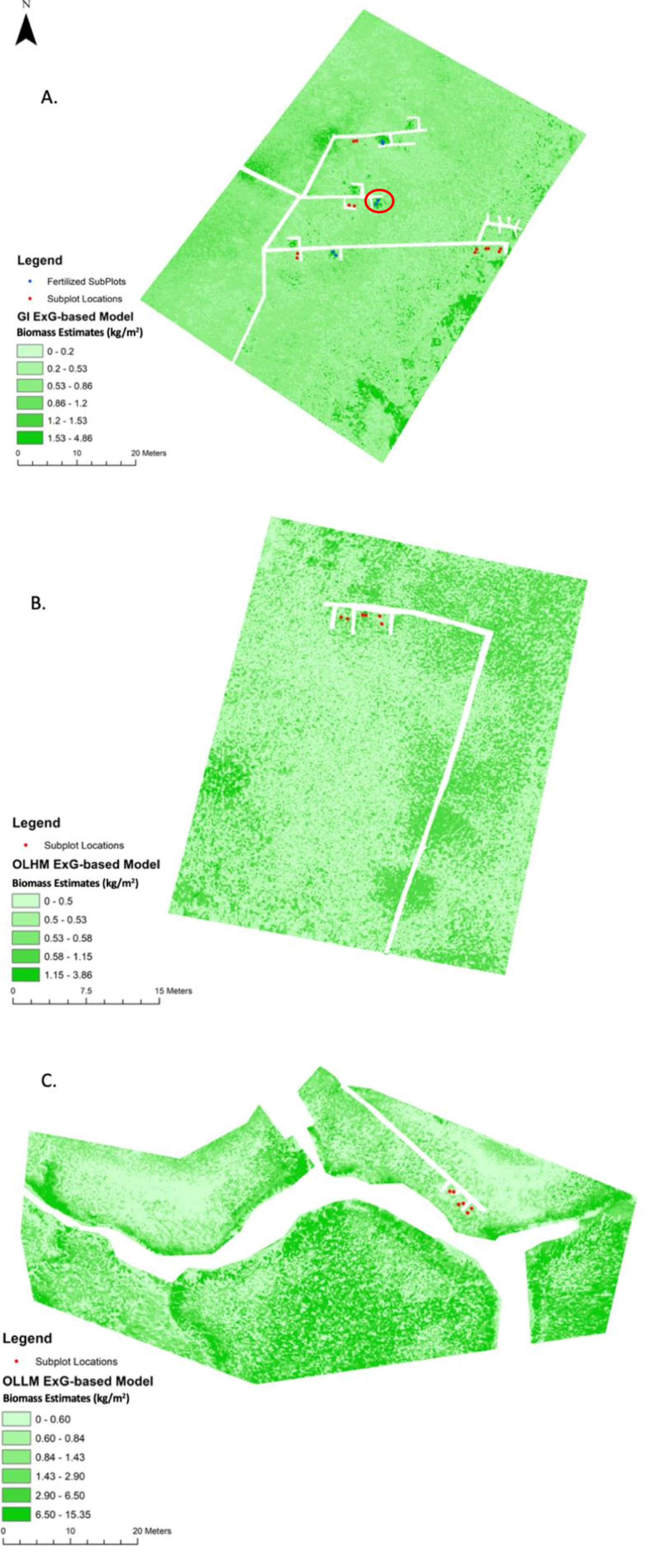
Biomass maps were created using the ExG-based biomass model (Equation (3)) at each study site in NIWB (Figure 9). A standard deviation histogram stretch was applied to the maps to accentuate the visual variability of biomass distributions in the maps. The real values of biomass were not changed. Only marsh pixels were mapped. Open water and man-made structures such as boardwalks were masked out. A minimum threshold of either two standard deviations below the mean or zero was used as the lower threshold of index values for input into the model. Although the areas should be low in biomass, negative index values would actually contribute to high biomass values on the map if not controlled. The histogram of index values varied depending upon the study site, but there were consistently exceptionally high ranges yet small means and standard deviations. Upper limits of index values derived from two standard deviations were used to control for extreme outliers presumably caused by atmospheric conditions and small pixel sizes that captured high variability.
At the GI site (Figure 9A), the estimated biomass ranged from 0–4.86 kg/m2. As a high marsh close to shore in the west (where the boardwalk is connected), biomass is relatively low across the site. The fertilized long-term LTREB plots show distinctively higher biomass than other areas in the high marsh. The biomass maps represent the fertilized plots very well; all three fertilized plots used in biomass data gathering are dark green on the GI map. The two subplots with extreme values in model development (as shown in Figure 8) are marked in Figure 9. Being fertilized and growing well, these two subplots reached biomass values of 3.63 kg/m2 and 2.99 kg/m2, respectively.
The six fertilized subplots (two per fertilized plot, the blue point marks in Figure 9A) show interesting trends. All six fertilized plots are high marsh at the GI site. Compared to all 20 of the biomass values used for model training across the three sites, two subplots show significantly higher biomass measurements, two show slightly higher measurements, and two show relatively low measurements throughout the year. For example, in August 2020, the highest two subplots were over 2.0 kg/m2 greater than the site average. The two slightly higher-than-normal measurements still were about 0.30–0.40 kg/m2 more than the site average. The last two fertilized subplots were 0.30 to 0.40 kg/m2 less than the average biomass measurements. Nevertheless, each of these subplots was on the high end of biomass for the GI environment, thus showing a dark green footprint compared to the other plots. Other plots that are not fertilized do not show up as well along the boardwalk section. Three other fertilized plots that are not used for this data-gathering research project are also visibly apparent.
The OLHM site (Figure 9B) is a typical high marsh close to shore in the south. Marshes are naturally grown without fertilizing experiments. Its biomass is generally low, in the range of 0–3.86 kg/m2. The marsh in the west of the boardwalk has homogeneously low biomass. Reasonably, areas further away from shore have increasing biomass.
The OLLM site (Figure 9C) is named a low marsh because its topography is lower than the other two sites, and it is further into the NIWB Estuary. The geomorphology of the site, the creek bank, a nearby causeway, and pier make the OLLM site unique. It is an area prone to wrack disturbances as well, compounded by the pier’s support pilings. Due to the accessibility, all biomass samples were collected in the north along the boardwalk, which may attribute to model misfitting in the typical low marsh. As shown in the figure, the maximal biomass reaches 15.35 kg/m2, which is unrealistically high and needs further investigation in the inner estuary.
Spatial patterns described in the literature [17,43], such as higher biomass along the tidal channels and in the low marsh of the inner estuary, are apparent in our maps. However, despite the recognizable patterns, the models significantly overestimate biomass as true biomass gets higher. When conducting model validation using the nine biomass samples, estimates of lower biomass from 0.3 to 0.9 kg/m2 had less absolute error (i.e., +0.006 to −0.42 kg/m2 absolute error) than the higher estimates (i.e., 1.95 kg/m2 error). For example, a fertilized subplot resulted in a 1.94 kg/m2 error between the observed value of 1.28 kg/m2 and the estimated value of 3.23 kg/m2. In contrast, an unfertilized plot resulted in a mere 0.0055 kg/m2 error between the observed value of 0.575 kg/m2 and the estimated value of 0.5695 kg/m2. In our future work, larger training and validation datasets will be collected for rectifying overestimation and recalibrating the model.
4. Discussion
RGB cameras are inexpensive and can be found on most off-the-shelf sUAS. The near-ubiquity of the visible-light cameras provides coastal managers with effective tools to map coastal wetlands. One of the benefits of sUAS-based remote sensing is that several types of environmental metrics can be estimated or obtained from a single sUAS flight, providing the means for a comprehensive environmental evaluation that can include metrics related to vegetation, sediment type, morphology, and much more for hard-to-reach areas [44,45,46]. Our study achieved similar results as those employing vegetation indices beyond visible spectra, for example, the normalized difference vegetation index (NDVI; R2 = 0.34) in a California coastal wetland [8]. This study enhances our understanding of RGB indices and their relationships with S. alterniflora biomass. While this study used a calibrated sensor with higher spectral sensitivity than the typical consumer-grade sUAS visible light camera, by focusing on the red, green, and blue bands, we were able to test the concept of using RGB imagery for biomass modelling. Future work will compare these results with inexpensive, more readily available sUAS and built-in cameras. Given the flexibility of consumer-oriented sUAS flights, the RGB index could serve as a quick tool for coastal managers to investigate marsh healthiness in small areas at high spatial and temporal resolutions.
This study unveils that the distance-based RGB indices perform better than the common ratio-based indices for biomass estimation of coastal marshes from sUAS imagery. Comparison analyses revealed that the excess green index (ExG) was the most suitable RGB index in this study, with a moderate non-linear relationship (R2 ≈ 0.4) and the biomass measured in the late summer during peak biomass. The ExG was originally created to map fractional vegetation cover, but it has also shown good results for other applications in numerous other studies [47]. It has also been shown to be sensitive to chlorophyll and nitrogen content, just like TGI [25]. The TGI was developed by [48] and has shown many strengths in various applications thus far. In a wetland environment, Ref. [24] mapped mangroves and successfully used TGI for separating vegetation classes from water and for estimating canopy cover. Though it partially overestimated canopy cover, it showed better sensitivity to vegetation than the visible atmospherically resistant index (VARI). Another found that TGI performed remarkably well for estimating hops canopy cover, just like the ExG [49]. Both indices perform well in many applications and are highly correlated because they are sensitive to the same vegetation elements. Of the two distance-based equations, we suggest ExG is the most useful for coastal managers for mapping biomass in tidal salt marshes because of the universal applicability of the equation. The equation used to create the ExG index simply relies on doubling the impact of the green band and then subtracting the red and blue bands. This can be applied to all environments without modification. TGI was originally found to be a strong indicator of chlorophyll content but also particularly sensitive to nitrogen fertilizing, which was performed on the fertilized plots. However, the TGI requires the use of empirically derived variables in the equation that may need adjustment for some environments. Furthermore, TGI was originally developed with hyperspectral imagery monitoring crops. ExG was originally developed for weed identification. It is of note that while TGI and ExG performed best during peak biomass, different indices may perform better at different times throughout the year. Future research will explore the use of RGB indices for biomass modelling during other seasons and S. alterniflora phenological states.
The stem height of salt marshes is highly correlated with vegetation dry weight [50]. The LTREB project at NIWB uses its own equation to estimate biomass from its monthly surveys of stem height [35,37]. However, the experiment in this study found that drone-extracted canopy height data (CHM) were not effective in modelling biomass. While the R2 of the height quadratic regression model was within the range presented by [9], the statistical relationship between CHM and the measured biomass was not significant. The CHM extraction in this study utilized the LiDAR data ground returns as bare earth surface, which was found to work well on terrestrial woodlands [51]. In coastal wetlands, however, studies [52,53,54] have reported on the poor performance of LiDAR elevation, which may introduce high uncertainties to CHM. Future work will be conducted with intensive field GNSS collection for better assessment of digital terrain models and digital surface models at our study site. Low marshes and high marshes can also be investigated separately to determine if elevation influences biomass modelling capabilities with sUAS.
It is important to address the modelling uncertainties. First, the ground biomass collection for training remote sensing-based biomass models has long been a destructive process. However, the biomass model training and validation data used for this study were non-destructively modelled from stem height measurements. Though the modelling equation used for biomass measurements has been shown to be very accurate, it is still modelled and therefore introduces another layer of uncertainty into the remote sensing model. These methods were proposed to attempt non-destructive means of sUAS remote sensing for biomass modelling. A comparison between destructive and non-destructive methods should be investigated to identify where and how much variability is added to the remote sensing modelling technique. Future work should also focus on incorporating larger training and validation samples to create a more robust model.
Wetlands can be difficult to map using remote sensing because of their complex nature. Environmental conditions can cause variability in reflectance. High tide was avoided to limit the amount of moisture in each image, but even at low tide, residual moisture can be visible in patches within the vegetation canopy. Furthermore, there are many tidal creeks present within NIWB that can be seen in some of the imagery. These tidal creeks are unavoidable and add to the complexity of mapping in wetlands. Cloud cover and wind were variable between missions. Although reflectance targets were imaged before and after flights, conditions during flights also changed slightly. A sensor placed on the sUAS facing the sun can be used to capture solar irradiance during the flight. One study [5] gathered data with such a sensor but did not use the data as they felt it caused an overestimation of NDVI values. We suggest investigating the impact of including a more comprehensive radiometric correction to improve sUAS-based biomass modelling of S. alterniflora.
A previous study has presented several flight configurations (i.e., flight altitude and overlap) and lighting conditions from sUAS flights and their effects on various products in a coastal wetland [55]. This study investigated the optimal RGB indices for practical use in estimating biomass measurements in a tidal marsh system. sUAS are being presented to coastal managers and professionals as a time-saving instrument for coastal wetland vegetation research [11,56]. These experiments, so far, have added support to these sentiments, though future research is required to continue the development of practical applications of sUAS for use in coastal environments.
5. Conclusions
As we continue into decades of sea-level rise and climate change that are predicted to significantly affect coastal tidal marshes, the development of efficient and effective monitoring practices is sorely needed. sUAS present coastal managers and researchers with cost-effective and on-demand tools for gathering data pertaining to several coastal tidal marsh vegetation health metrics. In this study, we demonstrated the utility of sUAS-extracted RGB visible light vegetation indices for modelling S. alterniflora biomass. The optimal index is the ExG index (RMSE = 0.598 kg/m2; R2 = 0.376). The extracted biomass maps fairly reflect the spatial variations of biomass at three marsh sites. Height metrics from the sUAS point cloud, relying on the LiDAR-derived bare earth model, did not significantly enhance our biomass models.
Author Contributions
G.R.M. and C.W.; methodology, G.R.M. and C.W.; software, G.R.M.; validation, G.R.M.; formal analysis, G.R.M.; investigation, G.R.M. and C.W.; resources, J.T.M., C.W., and G.R.M.; data curation, G.R.M., C.W., and J.T.M.; writing—original draft preparation, G.R.M.; writing—review and editing, G.R.M., C.W., and J.T.M.; visualization, G.R.M.; supervision, C.W.; project administration, C.W.; funding acquisition, C.W. All authors have read and agreed to the published version of the manuscript.
Funding
This research received no external funding.
Data Availability Statement
The S. alterniflora biomass data presented in this study are openly available in EDI Data Portal at https://0-doi-org.brum.beds.ac.uk/10.6073/pasta/5d94cd77d20121090c72bb81154ac302, accessed on 10 January 2021, reference number edi.135.5.
Acknowledgments
This work was partially supported by the ASPIRE-II Program from the Office of the Vice President for Research at the University of South Carolina (UofSC). The authors would like to thank Baruch Institute and NOAA National Estuarine Research Reserve for granting us access to the study area and field facilities. Special thanks to Karen Sundberg for her excellent feedback and comments on previous drafts, as well as Michael Hodgson and Steve Schill for their helpful comments during the development of the project. Finally, a special thank you to the anonymous reviewers for their outstanding feedback and suggestions.
Conflicts of Interest
The authors declare no conflict of interest.
References
- Loomis, M.J.; Craft, C.B. Carbon Sequestration and Nutrient (Nitrogen, Phosphorus) Accumulation in River-Dominated Tidal Marshes, Georgia, USA. Soil Sci. Soc. Am. J. 2010, 74, 1028–1036. [Google Scholar] [CrossRef]
- Ballard, J.; Pezda, J.; Spencer, D. An Economic Valuation of Southern California Coastal Wetlands. Master’s Thesis, University of California, Santa Barbara, CA, USA, 2016. [Google Scholar]
- Purcell, A.D.; Khanal, P.; Straka, T.; Willis, D.B. Valuing Ecosystem Services of Coastal Marshes and Wetlands; Land Grant Press: Clemson, SC, USA, 2020. [Google Scholar] [CrossRef]
- Thorne, K.; MacDonald, G.; Guntenspergen, G.; Ambrose, R.; Buffington, K.; Dugger, B.; Freeman, C.; Janousek, C.; Brown, L.; Rosencranz, J.; et al. U.S. Pacific coastal wetland resilience and vulnerability to sea-level rise. Sci. Adv. 2018, 4, eaao3270. [Google Scholar] [CrossRef] [Green Version]
- Kirwan, M.L.; Megonigal, P. Tidal wetland stability in the face of human impacts and sea-level rise. Nat. Cell Biol. 2013, 504, 53–60. [Google Scholar] [CrossRef]
- Sea Level Rise Adaptation Report Beaufort County, South Carolina. March 2015; SC Sea Grant Consortium Product #SCSGC-T-15-02. Available online: https://www.scseagrant.org/wp-content/uploads/Sea-Level-Rise-Adaptation-Report-Beaufort.pdf (accessed on 26 August 2021).
- Zhou, Z.; Yang, Y.; Chen, B. Estimating Spartina alterniflora fractional vegetation cover and aboveground biomass in a coastal wetland using SPOT6 satellite and UAV data. Aquat. Bot. 2018, 144, 38–45. [Google Scholar] [CrossRef]
- Doughty, C.L.; Cavanaugh, K.C. Mapping Coastal Wetland Biomass from High Resolution Unmanned Aerial Vehicle (UAV) Imagery. Remote Sens. 2019, 11, 540. [Google Scholar] [CrossRef] [Green Version]
- DiGiacomo, A.; Bird, C.; Pan, V.; Dobroski, K.; Atkins-Davis, C.; Johnston, D.; Ridge, J. Modeling Salt Marsh Vegetation Height Using Unoccupied Aircraft Systems and Structure from Motion. Remote Sens. 2020, 12, 2333. [Google Scholar] [CrossRef]
- Pinton, D.; Canestrelli, A.; Wilkinson, B.; Ifju, P.; Ortega, A. A new algorithm for estimating ground elevation and vegetation characteristics in coastal salt marshes from high-resolution UAV-based LiDAR point clouds. Earth Surf. Process. Landf. 2020, 45, 3687–3701. [Google Scholar] [CrossRef]
- Durgan, S.D.; Zhang, C.; Duecaster, A.; Fourney, F.; Su, H. Unmanned Aircraft System Photogrammetry for Mapping Diverse Vegetation Species in a Heterogeneous Coastal AWetland. Wetlands 2020, 40, 2621–2633. [Google Scholar] [CrossRef]
- Tiner, R.W. Introduction to Wetland Mapping and Its Challenges. In Remote Sensing of Wetlands: Applications and Advances, 1st ed.; Tiner, R.W., Lang, M.W., Klemas, V.V., Eds.; CRC Press: Boca Raton, FL, USA, 2015; pp. 43–65. [Google Scholar]
- Hardisky, M.; Klemas, V.; Daiber, F. Remote sensing salt marsh biomass and stress detection. Adv. Space Res. 1983, 2, 219–229. [Google Scholar] [CrossRef]
- Hardisky, M.; Smart, R.; Klemas, V. Seasonal spectral characteristics and aboveground biomass of the tidal marsh plant Spartina alterniflora. Remote Sens. Environ. 1983, 49, 85–92. [Google Scholar]
- Gross, M.F.; Klemas, V.; Levasseur, J.E. Remote sensing of biomass of salt marsh vegetation in France. Int. J. Remote Sens. 1988, 9, 397–408. [Google Scholar] [CrossRef]
- Zhang, M.; Ustin, S.L.; Rejmankova, E.; Sanderson, E.W. Monitoring Pacific Coast Salt Marshes Using Remote Sensing. Ecol. Appl. 1997, 7, 1039–1053. [Google Scholar] [CrossRef]
- Miller, G.J.; Morris, J.T.; Wang, C. Estimating Aboveground Biomass and Its Spatial Distribution in Coastal Wetlands Utilizing Planet Multispectral Imagery. Remote Sens. 2019, 11, 2020. [Google Scholar] [CrossRef] [Green Version]
- Jensen, J.R.; Coombs, C.; Porter, D.; Jones, B.; Schill, S.; White, D. Extraction of smooth cordgrass(spartina alterniflora)biomass and leaf area index parameters from high resolution imagery. Geocarto Int. 1998, 13, 25–34. [Google Scholar] [CrossRef]
- Jensen, J.R.; Olson, G.; Schill, S.R.; Porter, D.E.; Morris, J. Remote Sensing of Biomass, Leaf-Area-Index, and ChlorophyllaandbContent in the ACE Basin National Estuarine Research Reserve Using Sub-meter Digital Camera Imagery. Geocarto Int. 2002, 17, 27–36. [Google Scholar] [CrossRef]
- Klemas, V. Remote Sensing of Coastal Wetland Biomass: An Overview. J. Coast. Res. 2013, 290, 1016–1028. [Google Scholar] [CrossRef]
- Jensen, J.R. Drone Aerial Photography and Videography: Data Collection and Image Interpretation. Apple iBook. 2017. Available online: https://books.apple.com/us/book/drone-aerial-photography-and-videography/id1283582147 (accessed on 3 March 2021).
- Doughty, C.L.; Ambrose, R.F.; Okin, G.S.; Cavanaugh, K.C. Characterizing spatial variability in coastal wetland biomass across multiple scales using UAV and satellite imagery. Remote Sens. Ecol. Conserv. 2021. [Google Scholar] [CrossRef]
- Poley, L.G.; McDermid, G.J. A Systematic Review of the Factors Influencing the Estimation of Vegetation Aboveground Biomass Using Unmanned Aerial Systems. Remote Sens. 2020, 12, 1052. [Google Scholar] [CrossRef] [Green Version]
- Johnson, B.J.; Manby, R.; Devine, G. Performance of an aerially applied liquid Bacillus thuringiensis var. israelensis formulation (strain AM65-52) against mosquitoes in mixed saltmarsh–mangrove systems and fine-scale mapping of mangrove canopy cover using affordable drone-based imagery. Pest Manag. Sci. 2020, 76, 3822–3831. [Google Scholar] [CrossRef]
- Dale, J.; Burnside, N.; Hill-Butler, C.; Berg, M.; Strong, C.; Burgess, H. The Use of Unmanned Aerial Vehicles to Determine Differences in Vegetation Cover: A Tool for Monitoring Coastal Wetland Restoration Schemes. Remote Sens. 2020, 12, 4022. [Google Scholar] [CrossRef]
- Cen, H.; Wan, L.; Zhu, J.; Li, Y.; Li, X.; Zhu, Y.; Weng, H.; Wu, W.; Yin, W.; Xu, C.; et al. Dynamic monitoring of biomass of rice under different nitrogen treatments using a lightweight UAV with dual image-frame snapshot cameras. Plant Methods 2019, 15, 32. [Google Scholar] [CrossRef]
- Yue, J.; Yang, G.; Li, C.; Li, Z.; Wang, Y.; Feng, H.; Xu, B. Estimation of Winter Wheat Above-Ground Biomass Using Unmanned Aerial Vehicle-Based Snapshot Hyperspectral Sensor and Crop Height Improved Models. Remote Sens. 2017, 9, 708. [Google Scholar] [CrossRef] [Green Version]
- Maimaitijiang, M.; Sagan, V.; Sidike, P.; Maimaitiyiming, M.; Hartling, S.; Peterson, K.T.; Maw, M.J.; Shakoor, N.; Mockler, T.; Fritschi, F.B. Vegetation Index Weighted Canopy Volume Model (CVMVI) for soybean biomass estimation from Unmanned Aerial System-based RGB imagery. ISPRS J. Photogramm. Remote Sens. 2019, 151, 27–41. [Google Scholar] [CrossRef]
- Jing, R.; Gong, Z.; Zhao, W.; Pu, R.; Deng, L. Above-bottom biomass retrieval of aquatic plants with regression models and SfM data acquired by a UAV platform—A case study in Wild Duck Lake Wetland, Beijing, China. ISPRS J. Photogramm. Remote Sens. 2017, 134, 122–134. [Google Scholar] [CrossRef]
- Tait, L.; Bind, J.; Charan-Dixon, H.; Hawes, I.; Pirker, J.; Schiel, D. Unmanned Aerial Vehicles (UAVs) for Monitoring Macroalgal Biodiversity: Comparison of RGB and Multispectral Imaging Sensors for Biodiversity Assessments. Remote Sens. 2019, 11, 2332. [Google Scholar] [CrossRef] [Green Version]
- Fallati, L.; Saponari, L.; Savini, A.; Marchese, F.; Corselli, C.; Galli, P. Multi-Temporal UAV Data and Object-Based Image Analysis (OBIA) for Estimation of Substrate Changes in a Post-Bleaching Scenario on a Maldivian Reef. Remote Sens. 2020, 12, 2093. [Google Scholar] [CrossRef]
- Collin, A.; Dubois, S.; James, D.; Houet, T. Improving Intertidal Reef Mapping Using UAV Surface, Red Edge, and Near-Infrared Data. Drones 2019, 3, 67. [Google Scholar] [CrossRef] [Green Version]
- Morgan, G.R.; Hodgson, M.E. A Post-Classification Change Detection Model with Confidences in High Resolution Multi-Date sUAS Imagery in Coastal South Carolina. Int. J. Remote Sens. 2021, 42, 4309–4336. [Google Scholar] [CrossRef]
- Wyngaard, J.; Barbieri, L.; Thomer, A.; Adams, J.; Sullivan, D.; Crosby, C.; Parr, C.; Klump, J.; Shrestha, S.R.; Bell, T. Emergent Challenges for Science sUAS Data Management: Fairness through Community Engagement and Best Practices Development. Remote Sens. 2019, 11, 1797. [Google Scholar] [CrossRef] [Green Version]
- Morris, J.T.; Haskin, B. A 5-yr Record of Aerial Primary Production and Stand Characteristics of Spartina Alterniflora. Ecology 1990, 71, 2209–2217. [Google Scholar] [CrossRef]
- Ai, J.; Gao, W.; Gao, Z.; Shi, R.; Zhang, C. Phenology-based Spartina alterniflora mapping in coastal wetland of the Yangtze Estuary using time series of GaoFen satellite no. 1 wide field of view imagery. J. Appl. Remote Sens. 2017, 11, 26020. [Google Scholar] [CrossRef]
- Morris, J.; Sundberg, K. Environmental Data Initiative. LTREB: Aboveground Biomass, Plant Density, Annual Aboveground Productivity, and Plant Heights in Control and Fertilized Plots in a Spartina Alterniflora-Dominated Salt Marsh, North Inlet, Georgetown, SC: 1984–2020. 2021. Ver 5. Available online: https://0-doi-org.brum.beds.ac.uk/10.6073/pasta/5d94cd77d20121090c72bb81154ac302 (accessed on 8 July 2021).
- Davis, J.; Currin, C.; Morris, J.T. Impacts of Fertilization and Tidal Inundation on Elevation Change in Microtidal, Low Relief Salt Marshes. Chesap. Sci. 2017, 40, 1677–1687. [Google Scholar] [CrossRef]
- Digital Coast Data. Available online: https://coast.noaa.gov/digitalcoast/data/home.html (accessed on 20 March 2021).
- Possoch, M.; Bieker, S.; Hoffmeister, D.; Bolten, A.; Schellberg, J.; Bareth, G. Multi-Temporal Crop Surface Models Combined with the RGB Vegetation Index from UAV-Based Images for forage Monitoring in Grassland. ISPRS-Int. Arch. Photogramm. Remote Sens. Spat. Inf. Sci. 2016, XLI-B1, 991–998. [Google Scholar] [CrossRef] [Green Version]
- Michez, A.; Bauwens, S.; Brostaux, Y.; Hiel, M.-P.; Garré, S.; Lejeune, P.; Dumont, B. How Far Can Consumer-Grade UAV RGB Imagery Describe Crop Production? A 3D and Multitemporal Modeling Approach Applied to Zea mays. Remote Sens. 2018, 10, 1798. [Google Scholar] [CrossRef] [Green Version]
- Westoby, M.J.; Brasington, J.; Glasser, N.F.; Hambrey, M.J.; Reynolds, J.M. Structure-from-Motion photogrammetry: A low-cost, effective tool for geoscience applications. Geomorphology 2012, 179, 300–314. [Google Scholar] [CrossRef] [Green Version]
- Morris, J.T.; Porter, D.; Neet, M.; Noble, P.; Schmidt, L.; Lapine, L.A.; Jensen, J.R. Integrating LIDAR elevation data, multi-spectral imagery and neural network modelling for marsh characterization. Int. J. Remote Sens. 2005, 26, 5221–5234. [Google Scholar] [CrossRef]
- Dale, J.; Burgess, H.M.; Berg, M.J.; Strong, C.J.; Burnside, N.G. Morphological evolution of a non-engineered managed realignment site following tidal inundation. Estuar. Coast. Shelf Sci. 2021, 260, 107510. [Google Scholar] [CrossRef]
- Fairley, I.; Mendzil, A.; Togneri, M.; Reeve, D.E. The Use of Unmanned Aerial Systems to Map Intertidal Sediment. Remote Sens. 2018, 10, 1918. [Google Scholar] [CrossRef] [Green Version]
- Adade, R.; Aibinu, A.M.; Ekumah, B.; Asaana, J. Unmanned Aerial Vehicle (UAV) applications in coastal zone management—A review. Environ. Monit. Assess. 2021, 193, 1–12. [Google Scholar] [CrossRef] [PubMed]
- Woebbecke, D.M.; Meyer, G.E.; Von Bargen, K.; Mortensen, D.A. Color Indices for Weed Identification Under Various Soil, Residue, and Lighting Conditions. Trans. ASAE 1995, 38, 259–269. [Google Scholar] [CrossRef]
- Hunt, E.R.; Doraiswamy, P.C.; McMurtrey, J.E.; Daughtry, C.; Perry, E.M.; Akhmedov, B. A visible band index for remote sensing leaf chlorophyll content at the canopy scale. Int. J. Appl. Earth Obs. Geoinf. 2013, 21, 103–112. [Google Scholar] [CrossRef] [Green Version]
- Stary, K.; Jelinek, Z.; Kumhalova, J.; Chyba, J.; Balazova, K. Comparing RGB—Based vegetation indices from UAV imageries to estimate hops canopy area. Agron. Res. 2020, 18, 2592–2601. [Google Scholar]
- Davis, J.L.; Currin, C.A.; O’Brien, C.; Raffenburg, C.; Davis, A. Living Shorelines: Coastal Resilience with a Blue Carbon Benefit. PLoS ONE 2015, 10, e0142595. [Google Scholar] [CrossRef]
- Wang, C.; Morgan, G.; Hodgson, M. sUAS for 3D Tree Surveying: Comparative Experiments on a Closed-Canopy Earthen Dam. Forests 2021, 12, 659. [Google Scholar] [CrossRef]
- Enwright, N.M.; Wang, L.; Borchert, S.M.; Day, R.H.; Feher, L.C.; Osland, M.J. The Impact of Lidar Elevation Uncertainty on Mapping Intertidal Habitats on Barrier Islands. Remote Sens. 2017, 10, 5. [Google Scholar] [CrossRef] [Green Version]
- Wang, C.; Morgan, G.; Hodgson, M.E. Assessment of Elevation Uncertainty in Salt Marsh Environments using Discrete-Return and Full-Waveform Lidar. J. Coast. Res. 2016, 76, 107–122. [Google Scholar] [CrossRef]
- Hopkinson, C.; Chasmer, L.E.; Zsigovics, G.; Creed, I.F.; Sitar, M.; Treitz, P.; Maher, V. Errors in lidar ground elevation and wetland vegetation height estimates. Int. Arch. Photogramm. Remote Sens. Spat. Inf. Sci. 2004, 36, 108–113. [Google Scholar]
- Durgan, S.D.; Zhang, C.; Duecaster, A. Evaluation and enhancement of unmanned aircraft system photogrammetric data quality for coastal wetlands. GIScience Remote Sens. 2020, 57, 865–881. [Google Scholar] [CrossRef]
- Marcaccio, J.V.; Markle, C.E.; Chow-Fraser, P. Use of fixed-wing and multi-rotor unmanned aerial vehicles to map dynamic changes in a freshwater marsh. J. Unmanned Veh. Syst. 2016, 4, 193–202. [Google Scholar] [CrossRef]
Figure 1.
NIWB study site locations. South Carolina is located in the southeastern USA, bordering Georgia, North Carolina, and the Atlantic Ocean.
Figure 1.
NIWB study site locations. South Carolina is located in the southeastern USA, bordering Georgia, North Carolina, and the Atlantic Ocean.

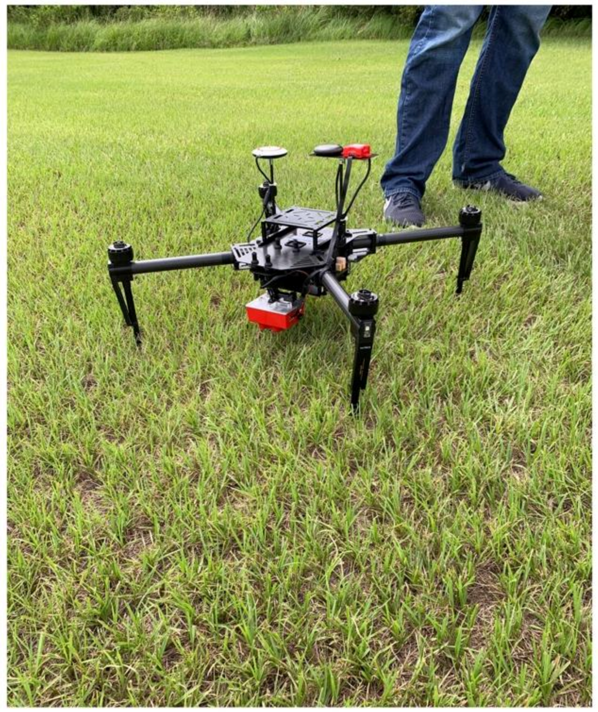
Figure 2.
The DJI Matrice 100 with the Micasense Red Edge-M multi-spectral camera.

Figure 3.
Emlid Reach GNSS base station (left) and rover (right) for collection of GCPs. (Top middle) image shows GCPs placed on the narrow boardwalk in various locations marked with red circles. (Bottom middle) image shows a black and white checkerboard GCP.
Figure 3.
Emlid Reach GNSS base station (left) and rover (right) for collection of GCPs. (Top middle) image shows GCPs placed on the narrow boardwalk in various locations marked with red circles. (Bottom middle) image shows a black and white checkerboard GCP.

Figure 4.
Example plot (bottom right) for ground biomass collection. The Emlid Reach RS2 base (not pictured) and rover were used to collect subplot centroid locations in March 2021. Centroid locations have not changed since 1984.
Figure 4.
Example plot (bottom right) for ground biomass collection. The Emlid Reach RS2 base (not pictured) and rover were used to collect subplot centroid locations in March 2021. Centroid locations have not changed since 1984.

Figure 5.
Example CHM for the GI site. Fertilized plots are represented by blue dots, and other non-fertilized plots are represented by red plots.
Figure 5.
Example CHM for the GI site. Fertilized plots are represented by blue dots, and other non-fertilized plots are represented by red plots.

Figure 6.
S. alterniflora average biomass curves derived from 29 subplots in NIWB over the year 2020. The peak biomass for each plot varies but ranges from late July to the beginning of October.
Figure 6.
S. alterniflora average biomass curves derived from 29 subplots in NIWB over the year 2020. The peak biomass for each plot varies but ranges from late July to the beginning of October.

Figure 7.
Visualization of the correlation matrix for all 10 RGB vegetation indices and canopy height.
Figure 7.
Visualization of the correlation matrix for all 10 RGB vegetation indices and canopy height.

Figure 8.
Scatterplots and Trendlines for each RGB index and Height metric with the training biomass data. R2 represents the coefficient of determination, and p values are indicated if the model was significant. Asterisks (*) indicate statistically significant models at 0.05.
Figure 8.
Scatterplots and Trendlines for each RGB index and Height metric with the training biomass data. R2 represents the coefficient of determination, and p values are indicated if the model was significant. Asterisks (*) indicate statistically significant models at 0.05.

Figure 9.
Biomass maps and sample point locations for GI (A), OLHM (B), and OLLM (C) using the ExG-based model. The two samples with the highest biomass (as shown in Figure 8) are circled in red in (A).
Figure 9.
Biomass maps and sample point locations for GI (A), OLHM (B), and OLLM (C) using the ExG-based model. The two samples with the highest biomass (as shown in Figure 8) are circled in red in (A).


Table 1.
Vegetation Indices computed for sUAS biomass modelling.
| Index | Formula | Reference 1 |
|---|---|---|
| ExG | 2 × G − R − B | [29] |
| GCC or Green Ratio | G/B + G + R | [27] |
| GRVI | (G − R)/(G + R) | [29] |
| IKAW | (R − B)/(R + B) | [28] |
| MGRVI | (G2 − R2)/(G2 + R2) | [26] |
| MVARI | (G − B)/(G + R − B) | [26] |
| RGBVI | (G2 − B × R)/(G2 + B × R) | [40] |
| TGI | G − (0.39 × R) − (0.61 × B) | [41] |
| VARI | (G − R)/(G + R − B) | [26] |
| VDVI or GLA | (2 × G − R − B)/(2 × G + R + B) | [26] |
1 These indices have been used in many other contexts and articles in the literature on biomass mapping. The authors recommend examining Poley and McDermid (2020) for a more extensive review.
Publisher’s Note: MDPI stays neutral with regard to jurisdictional claims in published maps and institutional affiliations. |
© 2021 by the authors. Licensee MDPI, Basel, Switzerland. This article is an open access article distributed under the terms and conditions of the Creative Commons Attribution (CC BY) license (https://creativecommons.org/licenses/by/4.0/).
Share and Cite
MDPI and ACS Style
Morgan, G.R.; Wang, C.; Morris, J.T. RGB Indices and Canopy Height Modelling for Mapping Tidal Marsh Biomass from a Small Unmanned Aerial System. Remote Sens. 2021, 13, 3406. https://0-doi-org.brum.beds.ac.uk/10.3390/rs13173406
AMA Style
Morgan GR, Wang C, Morris JT. RGB Indices and Canopy Height Modelling for Mapping Tidal Marsh Biomass from a Small Unmanned Aerial System. Remote Sensing. 2021; 13(17):3406. https://0-doi-org.brum.beds.ac.uk/10.3390/rs13173406
Chicago/Turabian StyleMorgan, Grayson R., Cuizhen Wang, and James T. Morris. 2021. "RGB Indices and Canopy Height Modelling for Mapping Tidal Marsh Biomass from a Small Unmanned Aerial System" Remote Sensing 13, no. 17: 3406. https://0-doi-org.brum.beds.ac.uk/10.3390/rs13173406
Note that from the first issue of 2016, this journal uses article numbers instead of page numbers. See further details here.