Detecting the Responses of CO₂ Column Abundances to Anthropogenic Emissions from Satellite Observations of GOSAT and OCO-2

Abstract

The continuing increase in atmospheric CO₂ concentration caused by anthropogenic CO₂ emissions significantly contributes to climate change driven by global warming. Satellite measurements of long-term CO₂ data with global coverage improve our understanding of global carbon cycles. However, the sensitivity of the space-borne measurements to anthropogenic emissions on a regional scale is less explored because of data sparsity in space and time caused by impacts from geophysical factors such as aerosols and clouds. Here, we used global land mapping column averaged dry-air mole fractions of CO₂ (XCO₂) data (Mapping-XCO₂), generated from a spatio-temporal geostatistical method using GOSAT and OCO-2 observations from April 2009 to December 2020, to investigate the responses of XCO₂ to anthropogenic emissions at both global and regional scales. Our results show that the long-term trend of global XCO₂ growth rate from Mapping-XCO₂, which is consistent with that from ground observations, shows interannual variations caused by the El Niño Southern Oscillation (ENSO). The spatial distributions of XCO₂ anomalies, derived from removing background from the Mapping-XCO₂ data, reveal XCO₂ enhancements of about 1.5–3.5 ppm due to anthropogenic emissions and seasonal biomass burning in the wintertime. Furthermore, a clustering analysis applied to seasonal XCO₂ clearly reveals the spatial patterns of atmospheric transport and terrestrial biosphere CO₂ fluxes, which help better understand and analyze regional XCO₂ changes that are associated with atmospheric transport. To quantify regional anomalies of CO₂ emissions, we selected three representative urban agglomerations as our study areas, including the Beijing-Tian-Hebei region (BTH), the Yangtze River Delta urban agglomerations (YRD), and the high-density urban areas in the eastern USA (EUSA). The results show that the XCO₂ anomalies in winter well capture the several-ppm enhancement due to anthropogenic CO₂ emissions. For BTH, YRD, and EUSA, regional positive anomalies of 2.47 ± 0.37 ppm, 2.20 ± 0.36 ppm, and 1.38 ± 0.33 ppm, respectively, can be detected during winter months from 2009 to 2020. These anomalies are slightly higher than model simulations from CarbonTracker-CO₂. In addition, we compared the variations in regional XCO₂ anomalies and NO₂ columns during the lockdown of the COVID-19 pandemic from January to March 2020. Interestingly, the results demonstrate that the variations of XCO₂ anomalies have a positive correlation with the decline of NO₂ columns during this period. These correlations, moreover, are associated with the features of emitting sources. These results suggest that we can use simultaneously observed NO₂, because of its high detectivity and co-emission with CO₂, to assist the analysis and verification of CO₂ emissions in future studies.

1. Introduction

Global atmospheric CO₂ concentration continues to increase by 2–3 ppm per year, which contributes significantly to global warming [1,2]. Changes in atmospheric CO₂ concentrations are primarily driven by emissions from human activities, photosynthesis of natural terrestrial ecosystems, and biogeochemical processes in the ocean. To achieve the goal of curbing global warming proposed by the Paris Agreement in 2015, many countries put forward the strategy of carbon neutrality. They are committed to limit global average temperature rise to be below 1.5° above pre-industrial levels through different effective ways of reducing greenhouse gas emissions [3,4]. To achieve these goals, it is critical to investigate the spatio-temporal changes of atmospheric CO₂ concentration and detect the influence mechanism of human activities in various regions on atmospheric CO₂ variations, so as to provide a basis for governments to evaluate the effects of CO₂ emission reduction measures.

Satellite measurements from GOSAT and OCO-2 have delivered the column-averaged dry air mole fractions of CO₂ (XCO₂) data for more than 12 years, which provide data for studying long-time variations of global and regional carbon emissions [5,6,7,8,9,10,11]. It has become an effective data source for understanding the contributions of natural ecosystems and human activities to the increase of atmospheric CO₂ concentration. For example, using satellite XCO₂ observations from GOSAT and OCO-2, many studies have found that extreme climate related to the El Niño Southern Oscillation (ENSO) disturbs the interannual increase of atmospheric CO₂ concentration at global and regional scales [12,13,14,15,16]. Abnormal increase in CO₂ concentration mostly occurs in natural vegetation areas. The detection and attribution analysis of extreme CO₂ changes show that CO₂ anomalies are related to the abnormal carbon emissions from terrestrial ecosystems caused by extreme climate [17]. Previous studies using CO₂ data from model and ground observations also showed consistent results with that from satellite observations [18,19,20,21,22].

XCO₂ enhancements could be detected by satellite observations in large cities, power plants, volcanoes, and fire emissions. By differencing the observations over a megacity with those in the nearby background, XCO₂ enhancements can be derived. The enhancement is found to be more than 3 ppm in large cities, such as Beijing-Tianjin-Hebei areas and the Yangtze River Delta in China, the Los Angeles megacity in the USA, the Seoul Metropolitan area in South Korea, and Mumbai in India [23,24,25,26,27,28,29]. XCO₂ observations from OCO-2 have also been used to identify enhanced plume signals and estimate anthropogenic emissions from individual point sources such as power plants and volcanoes [30,31,32]. For Australian mega bushfires, fire-induced XCO₂ enhancement detected by three orbits of observations from OCO-2 during November–December in eastern Australia is approximately 1.5 ppm [33]. Global XCO₂ anomalies derived from satellite observations agree well with the spatial patterns of emission inventories and model simulations [34,35,36]. Furthermore, an assessment combining satellite XCO₂ observations and other relatively short-lived pollutants (e.g., CO and NO₂) in cities found that urban CO₂ enhancements have a good correlation with air pollutants, which can be used to evaluate emission characteristics, such as combustion efficiency [36,37,38]. These results indicate that satellite XCO₂ observations have the detectability of natural and anthropogenic CO₂ emissions. Combined with ground-based measurements, they provide reliable data sources for constraining anthropogenic emission estimates and verifying bottom-up inventories.

However, previous studies on the detectivity of using satellite XCO₂ observations for anthropogenic emissions still have some limitations. Due to the impact of data sparsity in space and time caused by impacts from geophysical factors such as aerosols and clouds, most existing studies focus on individual areas or specific events, but lack sufficient analysis at global and regional scales. In response to this problem, we generated a dataset of global land mapping XCO₂ data (Mapping-XCO₂) using GOSAT and OCO-2 observations. With these global spatio-temporal continuous XCO₂ data, this study is able to fully explore the changes of XCO₂ enhancements caused by anthropogenic emission at both global and regional scales.

In this paper, we investigate global XCO₂ variations in space and time, and analyze spatial patterns of seasonal XCO₂ changes affected by atmospheric transport and terrestrial biosphere. We further focus on urban agglomerations with high anthropogenic emissions and quantify the responses of regional XCO₂ to anthropogenic emissions. Our study aims to provide global spatial and temporal analysis of XCO₂ changes and quantify the responses of regional XCO₂ enhancements to anthropogenic emission using long-term mapping data generated from satellite XCO₂ observations.

2. Materials and Methods

2.1. Materials

2.1.1. CO₂ Datasets

We use the global land mapping XCO₂ dataset (Mapping-XCO₂) from April 2009 to December 2020, which has a spatial grid resolution of 1° latitude by 1° longitude and temporal resolution of 3 days. The dataset is produced by applying a spatio-temporal geostatistical method to satellite XCO₂ retrievals from GOSAT observations (from April 2009 to August 2014) and OCO-2 observations (from September 2014 to December 2020). The XCO₂ retrievals are the latest ACOS level 2 Lite data product (v9r) and the latest level 2 lite data product (v10r) for OCO-2 [7,10,11]. These products are both obtained from the Goddard Earth Science Data Information and Services Center (GES DISC) [39]. The workflow chart of mapping gridded XCO₂ data are illustrated in Figure A1, including the following key steps: (1) We adjusted the differences in XCO₂ retrievals induced by the a priori CO₂ profile and different overpass time using CO₂ profiles from CarbonTracker as reference data. Spatial and temporal scales of satellite observations are integrated to a uniform unit by averaging XCO₂ within 10.5 km and 3 days. (2) The global land is divided into different continental regions and processed separately. In each mapping region, the spatio-temporal correlation structures of the integrated XCO₂ data are assumed to be homogeneous and locally stationary. The spatio-temporal empirical variogram in each region was calculated after removing the spatial and temporal trend from the integrated XCO₂. (3) Based on these variogram models, space-time kriging with moving cylinder kriging neighborhood was implemented to estimate the XCO₂ value at the center of 1° grids. A detailed description of the gap-filling method is referred to Zeng et al. [40,41,42,43] and He et al. [43]. We calculated estimation uncertainty for each grid according to the method described in Zeng et al. [42], which shows that the estimation uncertainty of Mapping-XCO₂ is less than 1.5 ppm on average. Compared to TCCON data, the overall bias of Mapping-XCO₂ obtained by ±0.5° box centered at the TCCON sites is 0.16 ± 1.19 ppm.

Table 1. The products of CO₂ data from satellite observation, model, and ground observation.

Dataset	Description	Reference/Data Source
Mapping-XCO2	Global land mapping XCO2 dataset produced by applying spatio-temporal geostatistics on GOSAT and OCO-2 observations from April 2009 to September 2020. The dataset is regularly distributed with a temporal interval of 3 days and spatial interval of 1° grid.	GES DISC [39] Zeng et al. [40,41,42,43]
CT-XCO2	The model XCO2 data at the local time 13:30 (LST) from CT 2019B from 2009 to March 2019 in 3° × 2° grids with a temporal interval of 1 day.	NOAA [45]
WDCGG-CO2	Global CO2 analysis based on ground-based observations, covering from 1984 to 2019 for global monthly mean concentrations and trends and from 1985 to 2018 for growth rates.	WDCGG [46]

gives a summary of Mapping-XCO₂ and the comparisons with model simulations by CarbonTracker and ground-based observations from the World Data Centre for Greenhouse Gases (WDCGG). CarbonTracker simulates global atmospheric CO₂ mole fractions from a combination of CO₂ surface exchange models and an atmospheric transport model driven by meteorological fields [44]. We collected CO₂ data at the local time of 13:30 from CT2019B for comparison analysis with spatio-temporal variations of Mapping-XCO₂. The dataset has a resolution of 3° × 2° grid in space and 1 day in time. In order to analyze long-term trends derived from Mapping-XCO₂, we collected global analysis data of atmospheric CO₂ concentrations and rates of change from WDCGG. The data are produced based on ground observations from the WMO Global Atmosphere Watch (GAW) in situ observational network. Globally averaged CO₂ mole fractions and CO₂ trends cover the period of 1984–2019, with the growth rates range from 1985 to 2018. These data are also reported by the annual WMO Greenhouse Gas Bulletin [2].

2.1.2. Auxiliary Datasets

To analyze the mechanism of XCO₂ changes and its response to anthropogenic emissions, we collected various auxiliary datasets to compare with XCO₂ variations at global and regional scales.

The Open-source Data Inventory for Anthropogenic CO₂ (ODIAC) is used to evaluate high emission areas, which can potentially be detected by satellite observed XCO₂ data. ODIAC is a global gridded emission product based on spatial and temporal disaggregation of country scale emissions [47,48]. The latest version of ODIAC emission data product (ODIAC 2020B) provides monthly CO₂ emissions from 2000 to 2019, including two different spatial resolutions of 1° × 1° and 1 km × 1 km. CO₂ emission estimates of the product are based on the latest country fossil fuel CO₂ emission estimates made by the new Carbon Dioxide Information Analysis Center (CDIAC) team from 2000 to 2017 and its projection using fuel consumption data reported by the BP Statistical Review of World Energy in 2018 and 2019 [49]. We downloaded ODIAC data from 2009 to 2019 from the Center for Global Environmental Research, National Institute for Environmental Studies (CGER-NIES) [49].

We used two ENSO indices, including the Southern Oscillation Index (SOI) and the Oceanic Niño Index (ONI), to analyze the fluctuating response of the global CO₂ growth rate to ENSO events. The indices are both provided by the Physical Sciences Laboratory at the National Oceanic and Atmospheric Administration (NOAA). The SOI is defined as the normalized pressure difference between Tahiti and Darwin based on the method developed by Ropelewski and Jones [50]. The data are obtained from the Climate Research Unit [51]. The ONI is a three-month running mean of sea surface temperature (SST) anomalies in the El Niño region (5°N–5°S, 120°W–170°W). The data are obtained from the NOAA Climate Prediction Center [52].

In order to evaluate the latitudinal zonal pattern of seasonal XCO₂ changes revealed by the satellite XCO₂ data, we compared it with the spatial patterns of potential temperature, which acts as a dynamical tracer of transport of the air masses [53]. Potential temperature is most frequently used in atmospheric sciences because it is not affected by the physical lifting or sinking associated with flow over obstacles or large-scale atmospheric turbulence [26,27,54]. Lines of constant potential temperature are natural flow pathways that are largely horizontal near the surface, and it is tightly correlated with CO₂ in simulations with zonally uniform surface fluxes [53]. In this paper, we used the potential temperature at 1000 hPa and calculated the averaged contours during the period from 2009 to 2020. The potential temperature data are monthly means produced by the NCEP/NCAR reanalysis. The online website is http://www.esrl.noaa.gov/psd/cgi-bin/data/composites/printpage.pl (accessed on 15 June 2021).

To analyze the influence of the terrestrial ecosystem on the global carbon cycle, we collected the Normalized Difference Vegetation Index (NDVI) data and the land cover type derived from the Moderate Resolution Imaging Spectroradiometer (MODIS) observation. These datasets are downloaded from the website https://ladsweb.modaps.eosdis.nasa.gov/ (accessed on 8 March 2021). NDVI data from the MOD13C2 product have temporal and spatial resolutions of 0.05° and 2 days, respectively [55]. We calculated global monthly mean data with 1° resolution from 2009 to 2020, which are used for correlation analysis with seasonal XCO₂ changes from Mapping-XCO₂. The land cover type is from the MCD12C1 product. We used the land cover type of the International Geosphere Biosphere Programme (IGBP) scheme, which includes 11 natural vegetation classes, 3 developed and mosaicked land classes, and 3 non-vegetated land classes. For regional studies, the land cover type is classified into urban, croplands, vegetation, and other.

NO₂ is a short-lived gas mostly co-emitted from fossil fuel combustion by industries and vehicles. It has been shown to be a good tracer for anthropogenic CO₂ emissions [36,37,38]. NO₂ data used in our studies is the level 3 offline NO₂ data product derived from TROPOMI/Sentinel-5 Precursor observations [56,57]. The data product provides the total vertical column of NO₂ concentrations with temporal and spatial resolutions of 2 days and 0.01° grid, respectively. The dataset is delivered by the European Space Agency (ESA) and publicly available on Google Earth Engine [57,58]. We obtained regional NO₂ columns in the study areas from July 2018 to December 2020 to assist the analysis of regional emission characteristics.

2.2. Methods

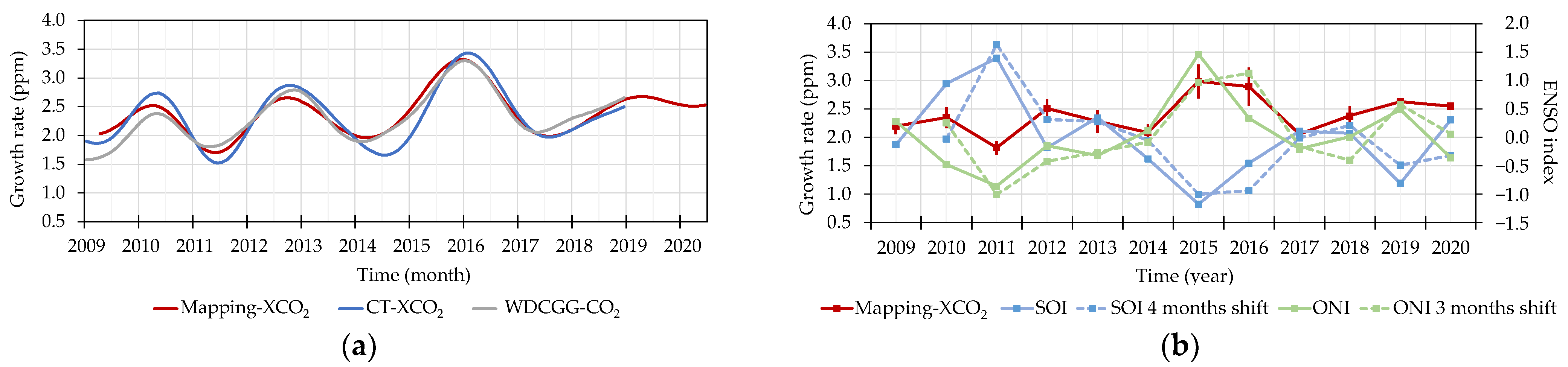
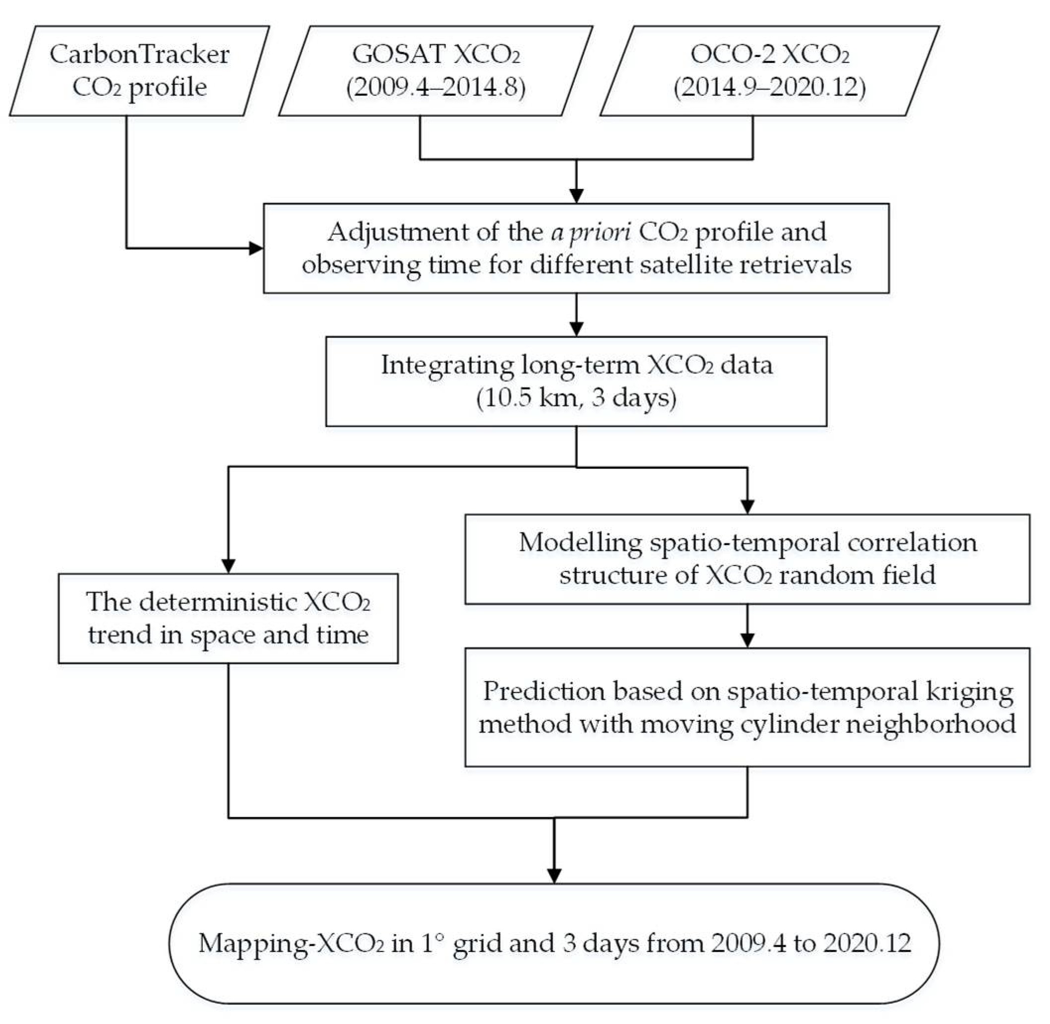
2.2.1. Calculation of Global Temporal XCO₂ Variations Using Mapping-XCO₂

The time series of atmospheric XCO₂ is basically a combination of three signals: a long-term trend, a seasonal cycle, and short-term variations [59]. To extract the temporal characteristics of XCO₂ variations, the most common method is to assume that the long-term trend and seasonal cycles can be represented by a polynomial function and a sum of seasonal harmonics, respectively [17,42,60,61,62]. As shown in Equation (1), we applied curve fitting to global gridded XCO₂ from Mapping-XCO₂ using a linear least squares regression method:

$$f\left(t\right)=a_0+a_{1}t+a_2{t}^2+{{\displaystyle \sum }}_{i=1}^4\left({\beta }_i\sin \left(i\omega t\right)+{\gamma }_i\cos \left(i\omega t\right)\right)$$

(1)

$$XC{O}_2=f\left(t\right)+\delta ,$$

(2)

where f(t) is the fitting result, t is the time in a unit of 3 days (122 cycles per year), ω is a parameter of the temporal period in yearly harmonics calculated by 2π/122. The parameters of $a_0,a_1, a_2, {\beta }_i,{\gamma }_i$ are obtained by least squares fitting. Note that the residuals ($\delta$) between global mapping XCO₂ data and f(t) in Equation (2) include a part of information on interannual and short-term variations that are not represented by the function. We use a low-pass filter to filter the residuals and obtain the signals of interannual and short-term variations [59,60]. Global monthly XCO₂ and its long-term trend are calculated by combining the fitting part of the function and the filtered part. The growth rate of global XCO₂ is computed by taking the derivative of the long-term trend of XCO₂.

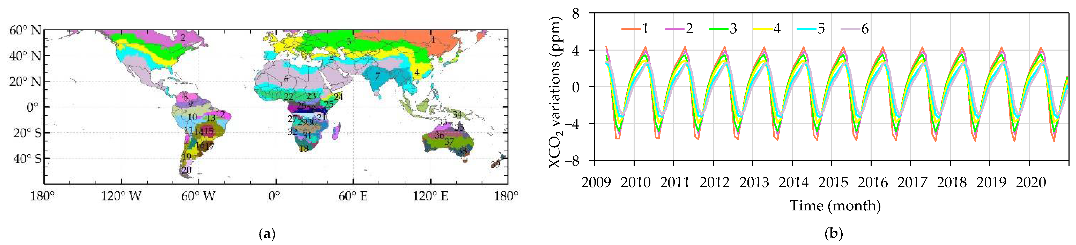
2.2.2. Clustering Spatial Pattern of the Seasonal XCO₂ Cycle

The changes of XCO₂ show a seasonal cycle especially in the Northern Hemisphere, which is affected by CO₂ flux from atmospheric transport and the terrestrial biosphere. The seasonal XCO₂ cycle for each grid is obtained by fitting XCO₂ timeseries of the grid using Equation (1), which also characterizes the long-term trend and a seasonal cycle for each grid. We utilized an unsupervised K-means method to cluster the XCO₂ based on the similarities in its seasonal cycles in order to obtain the spatial pattern of seasonal XCO₂ changes. K-means is an iterative algorithm used to classify the given dataset based on the similarity of temporally changing features where those grids with similar seasonal XCO₂ changes are classified into the same cluster [63]. The temporal variation of XCO₂, after removing long-term trends for each grid, reflects the biospheric fluxes from vegetation seasonal activities coupled with the atmospheric transport. This clustering method groups those grids with similar temporal variations to the same class. The clustering results are able to reveal the spatial patterns of atmospheric transport and terrestrial ecosystems’ CO₂ uptake.

2.2.3. Detecting CO₂ Anomalies at Global and Regional Scales

The global atmospheric CO₂ concentration represents a balance of all natural and anthropogenic CO₂ fluxes into and out of the atmosphere. Atmospheric CO₂ is well mixed by turbulent mixing and atmospheric transport [2]. We use global monthly averaged XCO₂ as the global background. Gridded XCO₂ anomalies are calculated as the differences between gridded XCO₂ data and the background, which is hereafter referred to as dXCO₂. The dXCO₂ is associated with net CO₂ fluxes in the grid. A negative dXCO₂ implies a net sink of CO₂, while positive dXCO₂ implies a net source relative to global background. The spatial distribution of global gridded dXCO₂ from Mapping-XCO₂ is described in Section 3.1 and is further compared with dXCO₂ from CT-XCO₂ data.

Lastly, we focus on urban agglomerations in China and the USA to demonstrate regional detectivity of CO₂ anomalies induced by anthropogenic emission. The urban agglomerations with high emissions are selected as study areas, which are basically located in the same latitude zone of 25°–45°. In order to remove large-scale CO₂ variations, median XCO₂ in the latitude zone is utilized as a background value. We computed regional XCO₂ anomalies(ΔXCO₂) by subtracting the “background” from regional averaged XCO₂ in the study areas.

3. Results

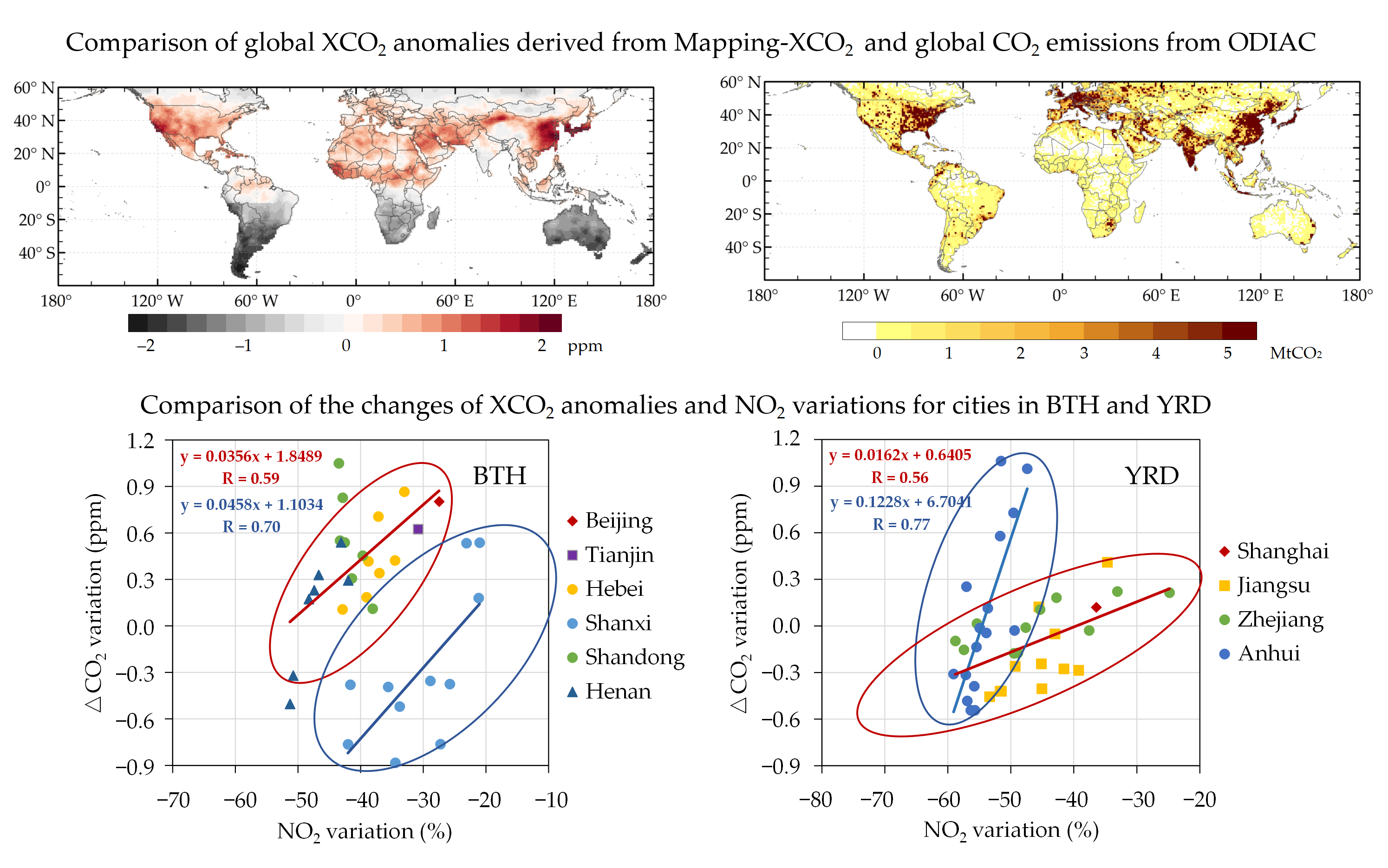
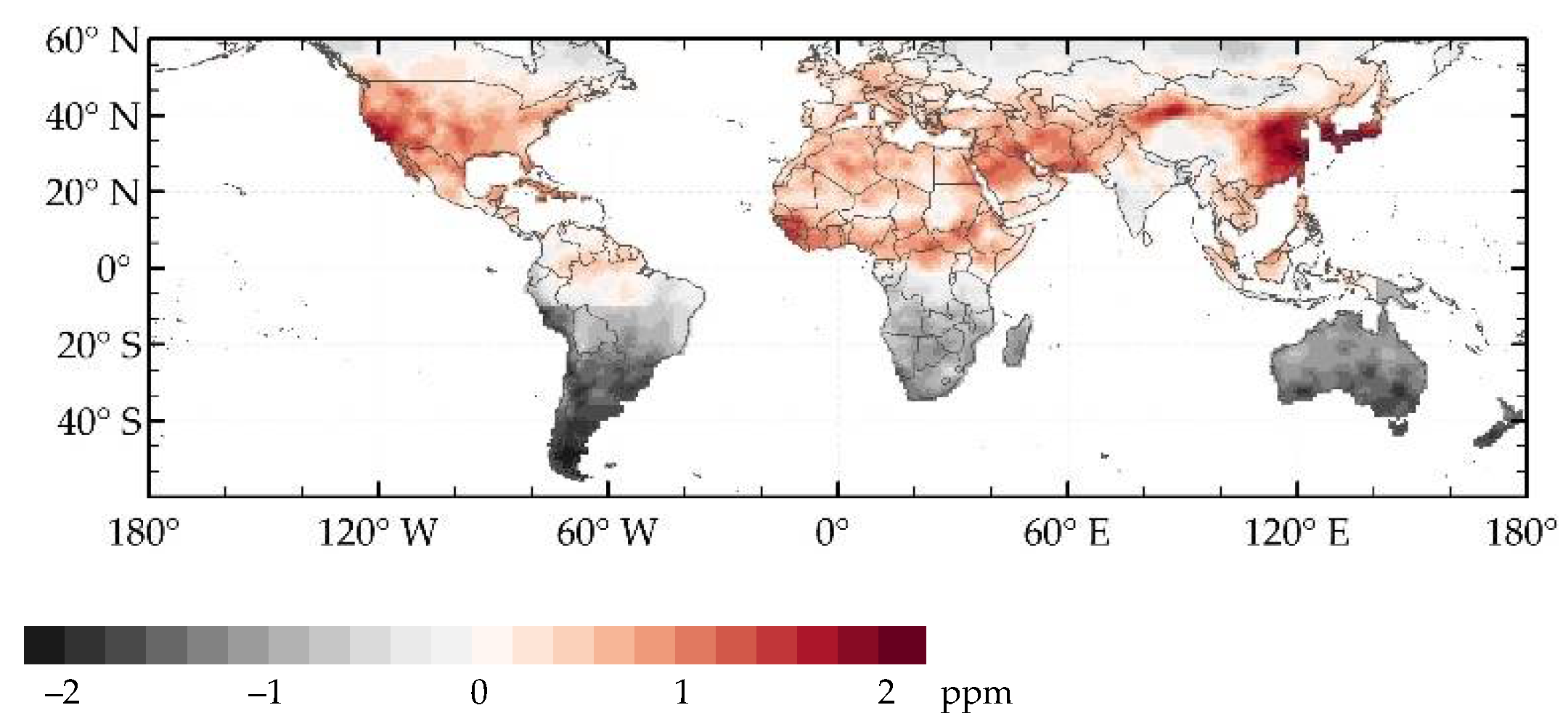
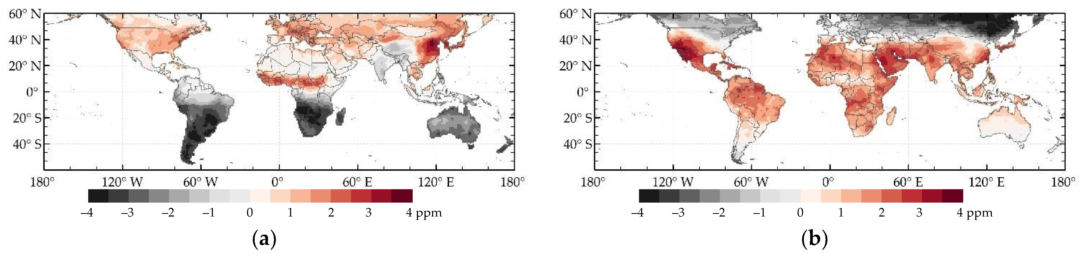
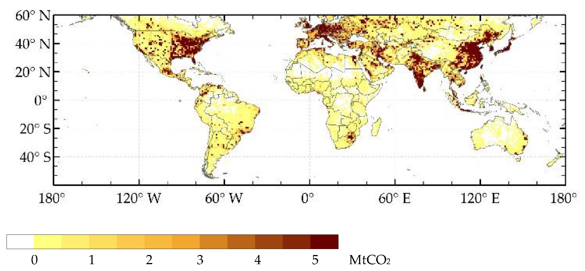
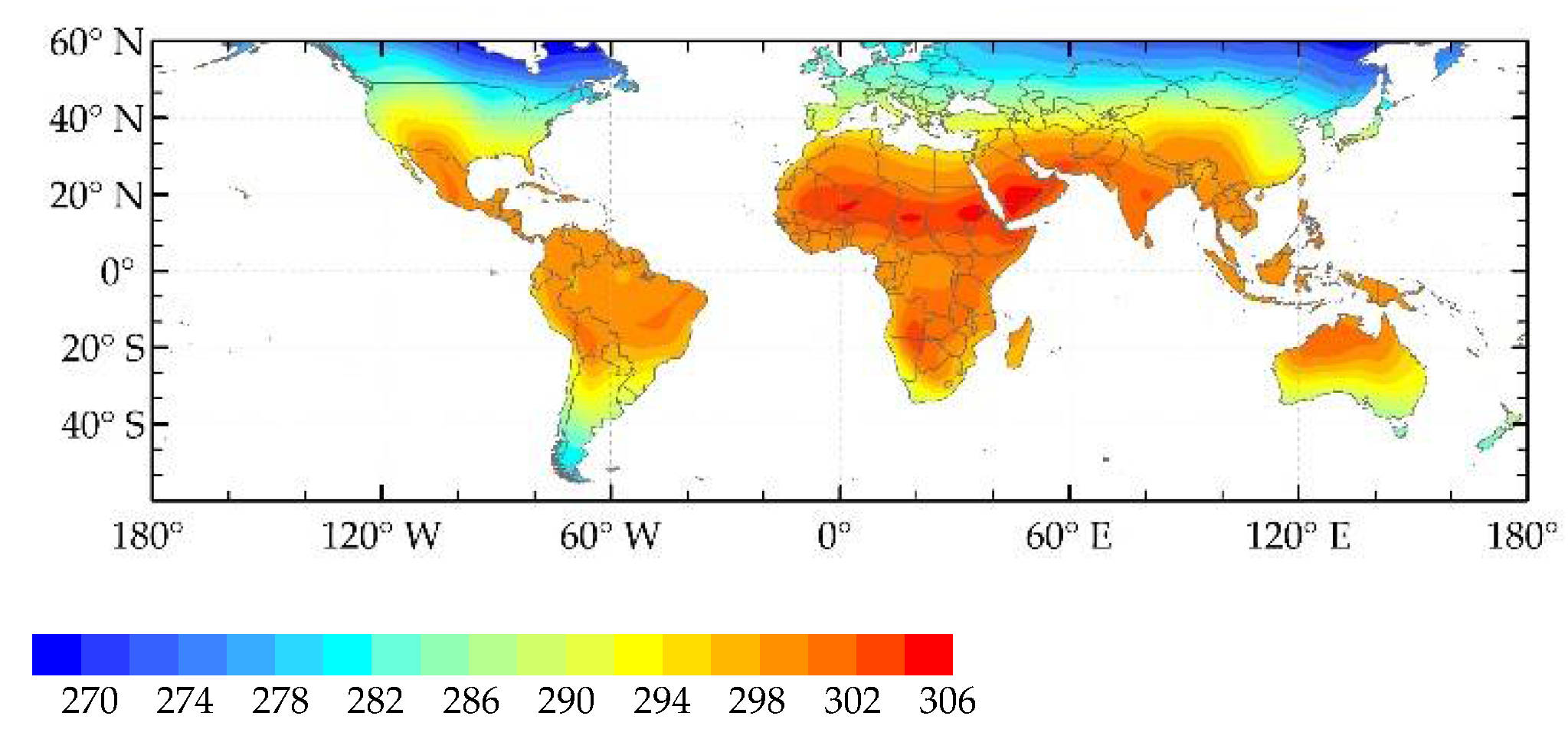
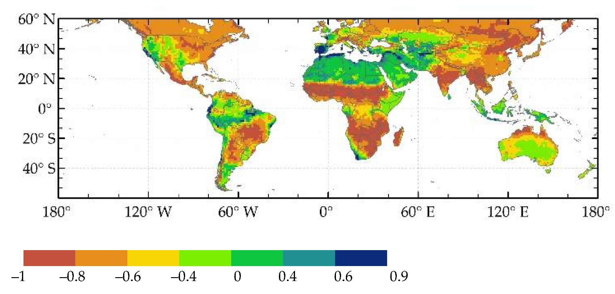
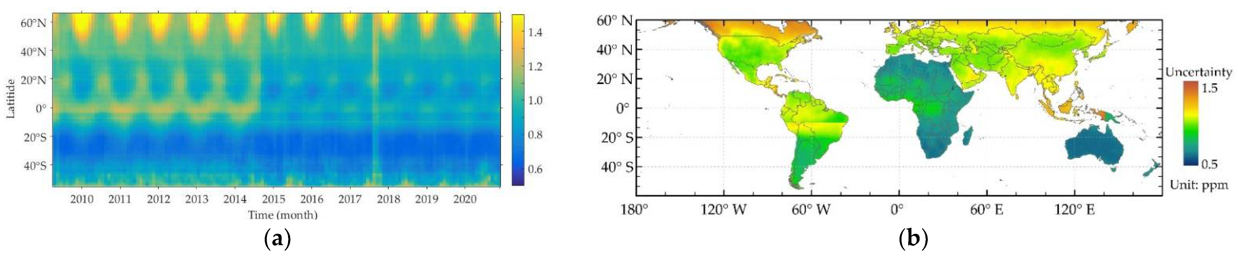
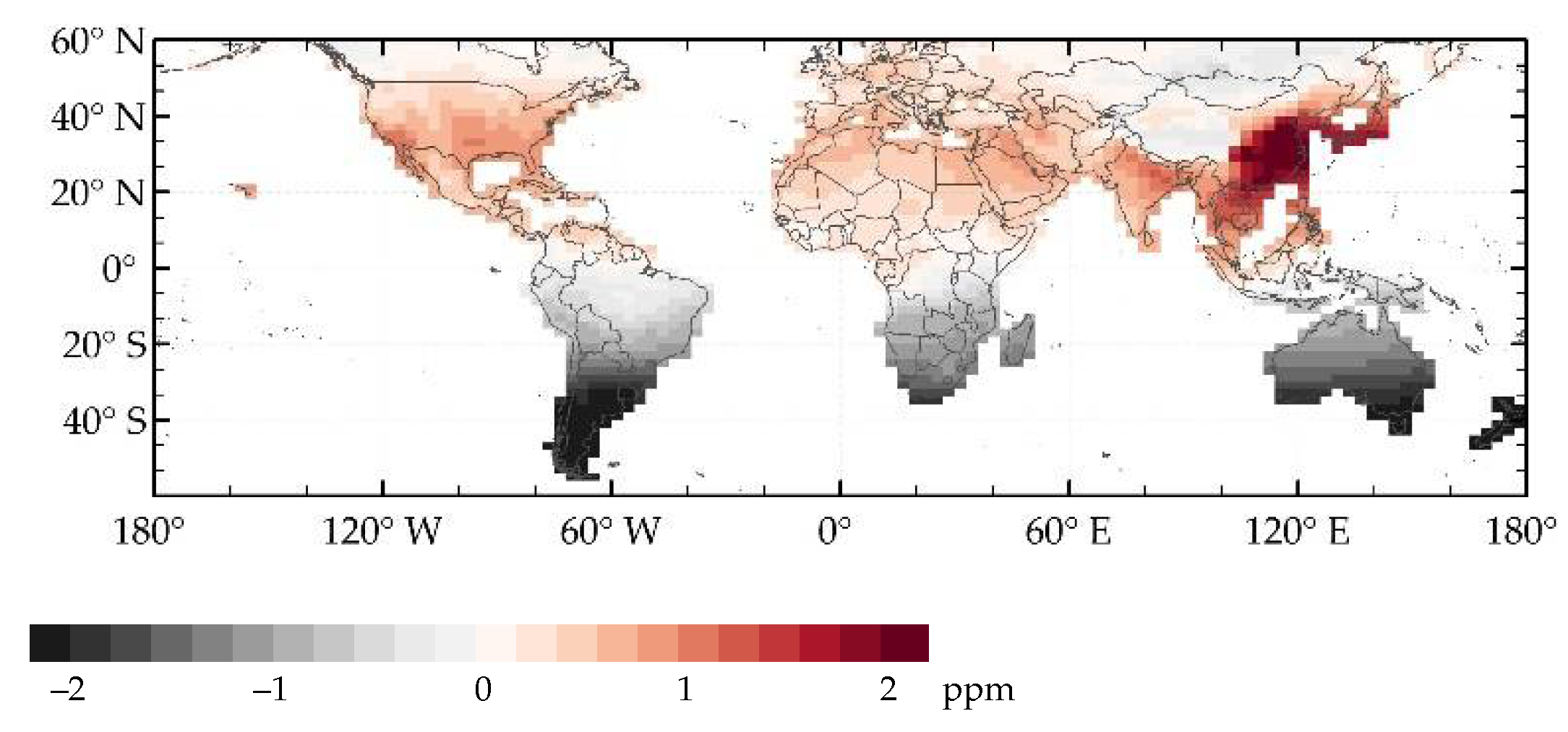
3.1. Spatio-Temporal Characteristic of Global XCO₂ Variations and Anthropogenic Emissions

We calculated global gridded anomalies (dXCO₂) from Mapping-XCO₂ and CT-XCO₂ to analyze global XCO₂ variations in space and time. Figure 1 shows spatial distributions of multi-year averaged dXCO₂ of Mapping-XCO₂ during 2010–2018, which have a similar spatial pattern with that calculated from CT-dXCO₂ in Figure A2. Higher positive dXCO₂ is observed in the region of East Asia, Southeast Asia, Middle East, North America, and North Africa. The dXCO₂ shows a negative value in the Southern Hemisphere. The result from Mapping-XCO₂ is about 0.4 ppm lower than CT-XCO₂ in eastern Asia. However, it shows obvious higher dXCO₂ over the regions of Xinjiang in China and lower dXCO₂ in India. The overall difference of global monthly mean XCO₂ between Mapping-XCO₂ and CT-XCO₂ is −0.24 ± 0.39 ppm, which is less than the difference of dXCO₂. Therefore, the differences of global XCO₂ anomalies between Mapping-XCO₂ and CT-XCO₂ are mostly induced by their gridded XCO₂ data. As can be seen in Figure A3, the large difference is mainly distributed in southern Eurasia. This large difference is very likely caused by sparse satellite observations that lead to higher mapping uncertainty, especially between 2010 and 2014.

Seasonal dXCO₂ in winter and summer are computed by averaging dXCO₂ values during December-January-February (DJF) and June-July-August (JJA), respectively. Figure 2 maps spatial patterns of seasonal dXCO₂ from Mapping-XCO₂ from 2009 to 2020. During wintertime, ecosystem CO₂ uptake tends to be minimal over the Northern Hemisphere so that the dXCO₂ is mostly caused by CO₂ emissions from fossil fuel combustions. Positive dXCO₂ of 1–2 ppm could be clearly observed in eastern China, eastern USA, and Europe in the Northern Hemisphere. The regions from the equator to 15° N have positive dXCO₂ values greater than 1 ppm in winter and lower dXCO₂ about 0.31 ppm in summer, which may be attributed to seasonal biomass burning [23,35,64]. In summer, the regions over the northern high latitudes show the largest negative dXCO₂ because terrestrial ecosystems in the Northern Hemisphere take up CO₂ emitted by human activities. CO₂ anomalies in the Southern Hemisphere are negative in winter and positive in summer, excluding the regions in tropical Africa. These spatial characteristics are generally similar to dXCO₂ calculated by CT-XCO₂ in Figure A4. Positive dXCO₂ in summer from CT-XCO₂ is slightly higher than the result of satellite XCO₂ data. The main difference is that there are no consistent changes of dXCO₂ in tropical Africa between Mapping-XCO₂ and CT-XCO₂, which may be due to the underestimation of fire emissions in CT simulation.

Comparing the spatial distribution of anthropogenic emissions from the ODIAC emission inventory in Figure 3, we can see that these regions with positive dXCO₂ of 1–2 ppm are very consistent with high anthropogenic emissions. As shown in Figure 2a and Figure A4a, the pattern of dXCO₂ in the United States during wintertime shows larger dXCO₂ in the east than that in the west, which is similar to the pattern of CO₂ emissions from ODIAC. Additionally, the high CO₂ absorption by natural terrestrial biosphere in the western region during summertime, because of the high emissions as indicated by ODIAC, is not found in the multi-year mean dXCO₂. These results indicate that global CO₂ anomalies in winter can effectively represent the increase in atmospheric CO₂ concentration caused by anthropogenic emissions and biomass burning.

Figure 4a shows the global CO₂ growth rates derived from Mapping-XCO₂, CT-XCO₂, and the ground-based CO₂ measurements from WDCGG. Compared with CT-XCO₂, the global CO₂ growth rates calculated by Mapping-XCO₂ are more consistent with observational data. Annual mean CO₂ growth rates of 1.82 to 2.98 ppm are reflected on the continuous increases in atmospheric CO₂ concentration, which is mainly caused by anthropogenic CO₂ emissions. High growth rates appeared in 2010, 2012/2013, and 2015/2016. Among them, the growth rate in 2015/2016 was the highest. Many studies have pointed out that significant inter-annual fluctuations are induced by abnormal natural CO₂ emissions associated with ENSO events [2,16]. For that, we also compared the annual CO₂ growth rate from Mapping-XCO₂ with two ENSO indices, which are shown in Figure 4b. The result shows the satellite-derived growth rates agree well with ENSO indices. The correlation of the annual CO₂ growth rate with SOI and ONI are −0.52 and 0.68, respectively. The growth rate response as quantified by the correlation coefficient (R) is largest after 4 months for SOI (R² = 40.24%) and after 3 months for ONI (R² = 58.46%). These results are consistent with previous reported findings [16,18,20,22].

3.2. Spatial Pattern of the Seasonal XCO₂ Cycle

Global seasonal XCO₂ changes from 2009 to 2020 are grouped into 40 clusters based on the K-means method as described in Section 2.2.2. Figure 5 presents spatial distribution of the clustering results. We noted that seasonal XCO₂ changes show latitudinal zonal distribution but significantly offset to the southwest in the Northern Hemisphere. These interesting results are highly consistent with the pattern of clusters derived from CT-XCO₂ using the same approach in Figure A5. Compared to the distribution of potential temperature in Figure 6, the spatial pattern of seasonal XCO₂ changes is in good agreement with potential temperature contours, especially in the Northern Hemisphere. The result indicates that clustered XCO₂ variation is relatively homogeneous, which allows us to detect any perturbations due to the external CO₂ fluxes within each cluster region. Moreover, seasonal amplitudes of XCO₂ gradually reduce from north to south as shown in Figure 5b. The maximum is up to 10 ppm in cluster 1, and the minimum is 5 ppm in cluster 5, which is primarily caused by the strength of vegetation uptake at different latitudes.

We further investigated the relationship between seasonal XCO₂ changes and seasonal vegetation activities characterized by NDVI. Figure 7 shows the spatial distribution of correlation coefficients (R) between their seasonal changes globally. The seasonal XCO₂ presents strong negative correlation with NDVI in most areas due to seasonal activities of vegetation CO₂ uptake in the northern high latitude area and regions of grassland and savannas. The regions with less or no vegetation present weak correlation between seasonal XCO₂ and NDVI. These regions with strong correlations indicate that the biosphere has large impacts on the variation of CO₂ concentration, which can also be seen in Figure A6.

An accurate assessment of the contribution of the biosphere and atmospheric transport helps better disentangle the contribution of anthropogenic emissions to XCO₂ variations. This clustering result can help us understand globally spatial distribution characteristics of XCO₂ variation affected by the biosphere and atmospheric transport. Comparing Figure 5a with Figure 6 and Figure 7, we can find that clustering results of XCO₂ after removing long-term changes effectively reveal the effects of fluxes from the biosphere and atmospheric transport. The ranges of clustering classes can be used to select and analyze interesting areas with similar biospheric fluxes and atmospheric transport.

3.3. Regional XCO₂ Anomalies and Anthropogenic Emissions

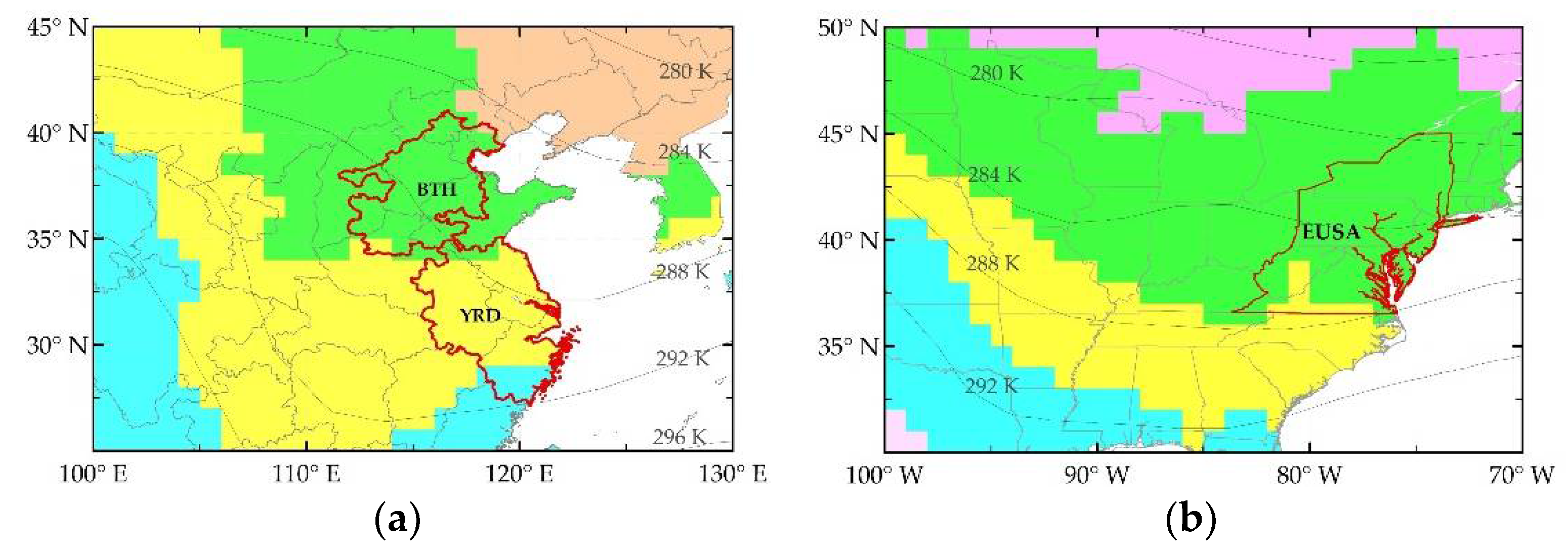
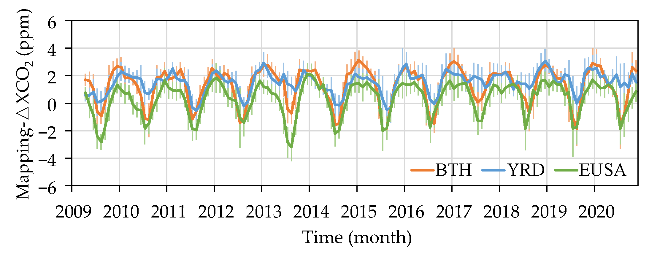
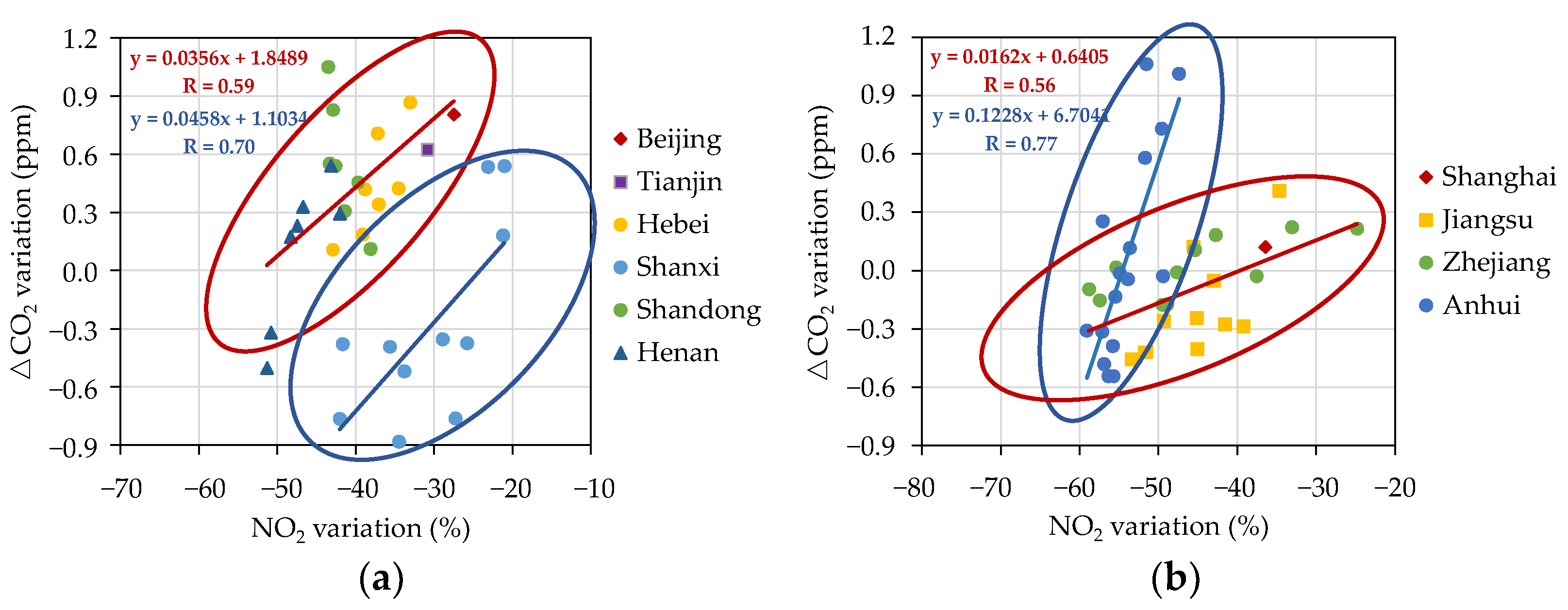
3.3.1. Regional XCO₂ Anomalies in Urban Agglomeration Areas

We focus on the investigation of regional XCO₂ anomalies caused by anthropo-genic emissions in the urban agglomeration areas in China and the United States. Based on the density of cities, we selected three source areas of anthropogenic emissions (AE), including the Beijing-Tian-Hebei region and nearby areas (BTH), the Yangtze River Delta urban agglomerations (YRD), and the urban agglomerations in the eastern United States of America (EUSA), which are shown in Figure 8. Total CO₂ emissions from these areas account for about 13% of global CO₂ emissions according to anthropogenic emissions from ODIAC. These three regions are located in the same clustering areas that have similar seasonal XCO₂ cycles. They are clusters 3 and 4, as shown in Figure 5.

Regional XCO₂ anomalies (ΔXCO₂) are calculated by removing the “background” trend of latitude zone from regional CO₂ concentrations as described in Section 3.1. We calculated the multi-year averaged ΔXCO₂ for these three regions using Mapping-XCO₂ according to two stages during 2009–2014 and during 2015–2020, respectively. From

Table 2. Regional characteristics in the emission source areas.

Source Areas	2009–2014			2015–2020
	BTH	YRD	EUSA	BTH	YRD	EUSA
XCO2 (ppm)	393.96 ± 3.55	394.14 ± 3.44	392.91 ± 3.56	407.56 ± 4.73	407.86 ± 4.87	406.77 ± 4.71
ΔXCO2 (ppm)	1.24 ± 0.24	1.42 ± 0.31	0.19 ± 0.19	1.36 ± 0.16	1.66 ± 0.22	0.57 ± 0.08
XCO2 in winter (ppm)	395.29 ± 3.49	395.12 ± 3.33	394.41 ± 3.55	409.40 ± 4.43	409.06 ± 4.56	408.14 ± 4.51
ΔXCO2 in winter (ppm)	2.32 ± 0.38	2.16 ± 0.34	1.44 ± 0.41	2.59 ± 0.33	2.25 ± 0.37	1.33 ± 0.25
Total CO2 emission (GtCO2/year)	1.54 ± 0.14	1.66 ± 0.04	0.72 ± 0.01	1.71 ± 0.19	1.86 ± 0.05	0.70 ± 0.01
Land cover (%) (Urban; Croplands; Vegetation; Other)	7.6	7.8	9.7	8.4	8.3	9.7
	34.9	56.4	13.5	34.5	55.4	14.1
	51.2	34.4	74.7	50.6	35.0	73.9
	6.3	1.4	2.2	6.6	1.5	2.3

, ΔXCO₂ are generally 1–3 ppm and the values during the wintertime are up to 1 ppm larger than the multi-year mean, especially for BTH and EUSA. Both BTH and EUSA are basically located in cluster 3 with a seasonal amplitude of 8 ppm, which is larger than the amplitude of 6 ppm for YRD in cluster 4. From the first 5 years of 2009–2014 to the second 5 years of 2015–2020, ΔXCO₂ increased in the three areas. Comparing the differences of ΔXCO₂ among AE areas, ΔXCO₂ in both BTH and YRD is greater than that in EUSA, while BTH is slightly larger than YRD.

Time series of XCO₂ anomalies in source areas from Mapping-XCO₂ and CT-XCO₂ are shown in Figure 9 and Figure A7, respectively. ΔXCO₂ shows seasonal variations in which BTH and EUSA present greater negative ΔXCO₂ than YRD. This is likely induced by the vegetation CO₂ uptake as the vegetation coverage is larger in BTH and EUSA. As can be seen from Figure 7, the correlation coefficients between seasonal CO₂ cycles and NDVI are −0.80 ± 0.11 and −0.77 ± 0.05 for BTH and EUSA, respectively, which are greater than the obtained coefficients of −0.65 ± 0.15 for YRD.

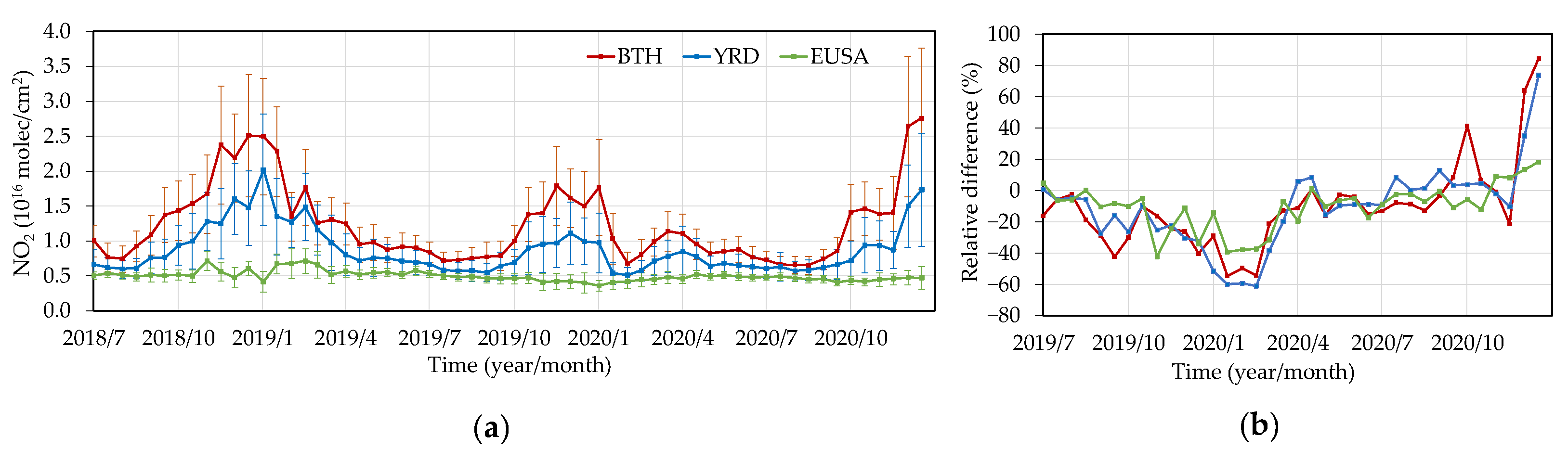
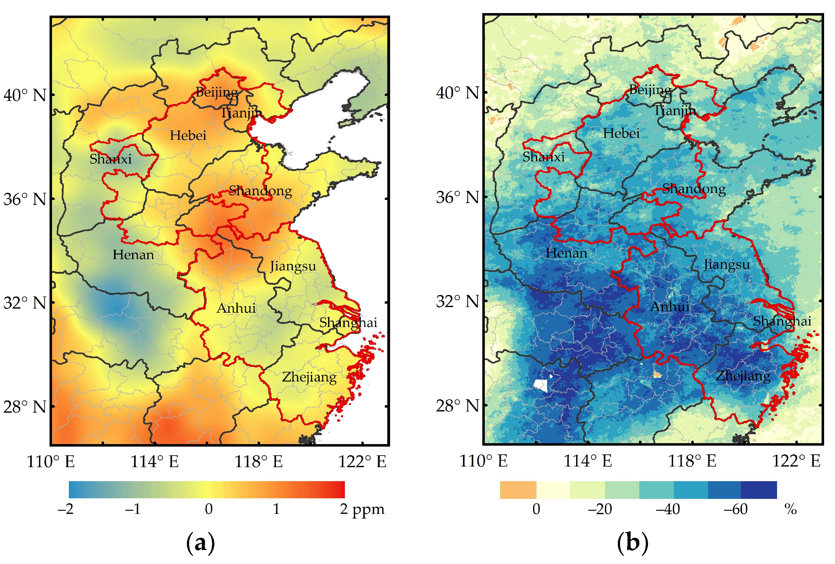
3.3.2. Response of Regional XCO₂ Anomalies during the COVID-19 Pandemic

Beginning from December 2019, Coronavirus disease 2019 (COVID-19) has occurred in numerous countries. The decline of economic activities caused by the pandemic lockdown measures has led to sharp reductions in anthropogenic CO₂ emissions in many countries. Regional-scale COVID-19-related CO₂ emission reductions are expected to be the largest in the first months of the pandemic outbreak. According to Le Quéré et al. [65], China’s CO₂ emissions decreased by 242 MtCO₂ (uncertainty range 108–394 MtCO₂) during January–April 2020. Buchwitz et al. [66] estimated the relative change of East China monthly emissions in 2020 relative to previous months. Their results showed significant differences across the ensemble of GOSAT and OCO-2 data products analysis. The ensemble mean indicates emission reductions by approximately 8% ± 10% in March 2020 and 10% ± 10% in April 2020 (uncertainties are 1-sigma), while somewhat lower reductions for the other months in 2020. These reduction months, however, should be investigated further, since the lockdown was mainly implemented during January–March; hence, the emission reduction should be in the same period.

We compared the relative differences of regional XCO₂ anomalies during January–April between 2020 and 2019. CO₂ anomalies in YRD have a slight decrease of 0.17 ppm during January to February in 2020 relative to the same month of 2019, while there has been no decline in CO₂ anomalies for BTH and EUSA. This is because that CO₂ is a long-lived gas, and therefore, it has a high background concentration in the atmosphere. The increase of CO₂ concentration caused by anthropogenic emissions and the decline induced by emission reduction are small variables. The precision of satellite observations and mapping uncertainty makes it difficult to detect weak signals due to the emission reduction.

NO₂ concentration in the atmosphere has been used to infer CO₂ reductions and estimate China’s CO₂ emissions during the COVID-19 pandemic [67]. Figure 10 illustrates the time series of regional NO₂ columns from July 2018 to December 2020 and the difference of 2020 relative to the previous year of 2019 for three areas. From Figure 10b, we can find that the sharp declines of NO₂ columns started in January and basically ended in April; NO₂ columns were reduced by 45–51%, 59%–61%, and 30% during January–March for BTH, YRD, and EUSA, respectively. The obvious reduction during the lockdown indicates that NO₂ columns are more sensitive to the reduction of anthropogenic emissions. The reduction, moreover, is lower in BTH than in YRD. This likely implies that the effects of reduced emissions from the decreased traffic volume were due to lockdown measures in YRD. However, there was increased demand for winter heating in BTH, as more people in 2020 had to stay in Beijing during the lockdown compared to former years. Additionally, the BTH area suffered a heavy pollution process from 11–13 February during the lockdown period [68].

In order to further analyze the response of XCO₂ to emission reduction in BTH and YRD, we focused on the period from January to March and compared the differences between 2019 and 2020 for ΔXCO₂ and NO₂ columns. ΔXCO₂ was resampled to a 0.01° grid by cubic convolution, which improves spatial resolution without changing the characteristics of the original data. As shown in Figure 11, the differences of ΔXCO₂ between 2020 and 2019 tend to be negative in YRD, which means that emissions reduced, while they tended to increase by approximately 0.5 to 1 ppm in BTH. The spatial pattern of differences for ΔXCO₂ is generally similar to NO₂ columns. The decrease of NO₂ columns in BTH is less than that in YRD. The NO₂ concentration decreased by approximately 35 ± 5% in BTH, while it decreased by approximately 45 ± 8% in YRD.

In addition, we computed the variations of ΔXCO₂ and NO₂ columns using the city district as a spatial unit. Figure 12 shows the result where the cities in AE areas are grouped according to provinces. The relationship between ΔXCO₂ and NO₂ shows two distinct features in both BTH and YRD, Shanxi and other provinces in BTH, and Anhui and the other provinces in YRD. These features are likely related to the types of emitting sources in these areas. The emitting sources in Shanxi and Anhui are mostly coal power plants and chemical plants, while the emitting sources of other provinces are mostly gas power plants and vehicles in the megacities of Beijing and Tianjin in BTH and Shanghai, Nanjing, Hangzhou, etc. in YRD. In Shanxi, the reduction of ΔXCO₂ is from −0.3 to −0.9 ppm and the decline of NO₂ is 35% to 42%. In BTH, the reduction of ΔXCO₂ is approximately 0.3 to 0.9 ppm and the decline of NO₂ is 30% to 45%. In comparison, in YRD, there is a larger range of ΔXCO₂ changes, from approximately −0.6 to 1 ppm with declines of NO₂ by 50% to 66% in Anhui. However, for other provinces in YRD other than Anhui, there are smaller changes of ΔXCO₂ from approximately −0.5 to 0.3 ppm, with a decline of NO₂ by 30% to 45%. These results indicate that the relationship between XCO₂ and NO₂ is available for the estimation of CO₂ emissions. However, we should also consider the regional features of emitting sources, since their relationship highly depends on the types of emitting sources.

4. Discussion

The accuracy of used Mapping-XCO₂ data will result in uncertainty around the findings of the spatio-temporal feature analysis. As described in Section 2.1.1, Mapping XCO₂ data are obtained by processing different satellite observations using the spatio-temporal geostatistical method. The mapping uncertainty depends not only on the retrieval bias of original XCO₂ retrievals, but also to a large extent on the number of available satellite observations. Mapping uncertainties are calculated by the method of Zeng et al. [43,44,45,46]. Figure 13 shows the spatio-temporal distribution of mapping uncertainties. The mapping uncertainties of global grids are generally less than 1.5 ppm. The areas with larger uncertainties are mainly in the high latitude of the Northern Hemisphere, which is due to sparse satellite observations. Mapping uncertainties during the period of GOSAT observations is higher than that corresponds to OCO-2 observations. This is because that the number of GOSAT observations is much less than OCO-2 observations. In the global analysis, CO₂ growth rates derived from Mapping-XCO₂ during 2009 to 2020 are consistent with that from ground-based measures, which does not show the deviation, such as the uncertainty between GOSAT and OCO-2 data. The spatial patterns of mapping gridded XCO₂, in contrast to the global background, are consistent from year to year. These results indicate that the mapping XCO₂ dataset using different satellite observations has consistent distribution characteristics in space and time. Moreover, the relative difference between regional XCO₂ in source areas and the global background is in the range of 1.13 to 3.17 ppm during winter months, which is greater than mapping uncertainty in these areas.

The land cover types in AE areas are dominated by croplands and vegetation, as shown in Table 2. Affected by the CO₂ uptake of terrestrial ecosystems and the accumulation of CO₂ from anthropogenic CO₂ emissions in the atmosphere, the regional CO₂ concentration reaches the highest value in the spring. The method of CO₂ anomalies can remove large-scale background information from regional CO₂ concentrations and enhance the signal of CO₂ changes. Many studies have pointed out that the calculation method of background concentration does not have a great impact on the results of regional CO₂ anomalies [35]. The temporal characteristic of regional CO₂ anomalies is consistent with that of the regional NO₂ concentration, as shown in Figure 10. Both of them have a maximum during the winter period of each year.

Regional CO₂ anomalies are mainly caused by anthropogenic CO₂ emissions and local ecological CO₂ fluxes. Regional ecological CO₂ flux has little impact on CO₂ changes in winter; CO₂ enhancement is in the range of 1.00 to 3.14 ppm in source areas during winter months, whereas the mapping uncertainty is 0.75 to 1.42 ppm in the same period. During the winter period, ΔXCO₂ of BTH is higher than that of YRD, which agrees with the emission characteristics of NO₂ concentrations. The ΔXCO₂ in BTH and EUSA show negative values in summer, which is because local ecological CO₂ fluxes have a greater impact on CO₂ anomalies in summer. On the other hand, the mapping uncertainty and standard deviation are relatively larger during the summer months. Therefore, it is challenging to detect the enhancement of regional CO₂ concentration caused by anthropogenic emissions in the growing season of vegetation.

5. Conclusions

We presented a global analysis of spatio-temporal XCO₂ variations and detected regional XCO₂ anomalies using satellite mapping XCO₂ data (Mapping-XCO₂) from April 2009 to December 2020. The dataset has resolutions of 3 days in time and 1° grid in space, respectively. Mapping-XCO₂ is produced by a gap-filling technique using XCO₂ retrievals obtained by GOSAT and OCO-2.

The growth rates of global XCO₂ derived from Mapping-XCO₂ data show large fluctuations in inter-annual variabilities, which is in agreement with the long-term CO₂ trends calculated by WDCGG ground-based observations. Elevated XCO₂ of 1.5 to 3.5 ppm, which is mostly induced by anthropogenic emissions and seasonal biomass burning, can be observed using Mapping-XCO₂ data with background removed. Furthermore, the clustering analysis of gridded seasonal XCO₂ variations, after removing the long-term trend and background, reveal spatial pattern of atmospheric transport and terrestrial ecological CO₂ flux.

At the regional scale, XCO₂ enhancements during winter months are detected to be 2.47 ± 0.37 ppm, 2.20 ± 0.36 ppm, and 1.38 ± 0.33 ppm for the Beijing-Tianjin-Hebei area, the Yangtze River Delta area, and the high-density urban areas in the eastern USA, respectively. The regional emission characteristic of XCO₂ enhancement is consistent with regional NO₂ columns. However, it is difficult to accurately detect enhanced CO₂ signals in the vegetation growing season due to impacts of local ecological CO₂ uptakes and relatively large uncertainty of the mapping data during summertime. The regional XCO₂ anomalies did not clearly show the declines of anthropogenic CO₂ emissions during the lockdown of the COVID-19 pandemic from January to March 2020 compared with the same time in the previous year of 2019. However, the significant correlation between relative differences of XCO₂ and NO₂ columns calculated at urban scales indicates that different types of emitting sources show a significantly positive correlation. This result suggests that we could use space-observed NO₂ data to identify the anthropogenic emitting sources and rectify CO₂ emissions estimated from satellite observations since both gases are mostly co-emitted in cities.

Our studies provide new cases for investigating the responses of XCO₂ observed by satellites to anthropogenic emissions at global and regional scales. These results demonstrate the potential of the global land mapping XCO₂ dataset in monitoring the long-term XCO₂ variations and detecting regional XCO₂ enhancements caused by anthropogenic in non-growing seasons.

References

1. Friedlingstein, P.; O’Sullivan, M.; Jones, M.W.; Andrew, R.M.; Hauck, J.; Olsen, A.; Peters, G.P.; Peters, W.; Pongratz, J.; Sitch, S.; et al. Global Carbon Budget 2020. Earth Syst. Sci. Data 2020, 12, 3269–3340. [Google Scholar] [CrossRef]
2. World Meteorological Organization. WMO Greenhouse Gas Bulletin No. 16. 2020. Available online: https://www.eenews.net/assets/2020/11/23/document_ew_05.pdf (accessed on 2 March 2021).
3. Coulter, L.; Canadell, J.; Dhakal, S. Global Carbon Project Report No. 6, Earth System Science Partnership Report No. 5, Canberra. Global Carbon Project (2008) Carbon Reductions and Offsets. Available online: https://www.globalcarbonproject.org/carbonneutral/index.htm (accessed on 22 February 2021).
4. Defining Carbon Neutrality for Cities & Managing Residual Emissions. Available online: https://www.c40.org/researches/defining-carbon-neutrality-for-cities-managing-residual-emissions (accessed on 31 January 2021).
5. GOSAT Project. Available online: www.gosat.nies.go.jp (accessed on 1 June 2020).
6. Orbiting Carbon Observatory. Available online: https://ocov2.jpl.nasa.gov (accessed on 1 June 2020).
7. Crisp, D.; Frankenberg, C.; Messerschmidt, J.; Wennberg, P.O.; Wunch, D.; Yung, Y.L. The ACOS CO2 retrieval algorithm—Part II: Global XCO2 data characterization. Atmos. Meas. Tech. 2012, 5, 687–707. [Google Scholar] [CrossRef] [Green Version]
8. Nakajima, M.; Kuze, A.; Suto, H. The current status of GOSAT and the concept of GOSAT-2. Proc. SPIE 2012, 8533, 853306. [Google Scholar] [CrossRef]
9. Kataoka, F.; Crisp, D.; Taylor, T.E.; O’Dell, C.W.; Kuze, A.; Shiomi, K.; Suto, H.; Bruegge, C.; Schwandner, F.M.; Rosenberg, R. The cross-calibration of spectral radiances and cross-validation of CO2 estimates from GOSAT and OCO-2. Remote Sens. 2017, 9, 1158. [Google Scholar] [CrossRef] [Green Version]
10. O’Dell, C.W.; Eldering, A.; Wennberg, P.O.; Crisp, D.; Gunson, M.R.; Fisher, B.; Frankenberg, C.; Velazco, A. Improved retrievals of carbon dioxide from Orbiting Carbon observatory-2 with the version 8 ACOS algorithm. Atmos. Meas. Tech. 2018, 11, 6539–6576. [Google Scholar] [CrossRef] [Green Version]
11. Kiel, M.; O’Dell, C.W.; Fisher, B.; Eldering, A.; Nassar, R.; MacDonald, C.G.; Wennberg, P.O. How bias correction goes wrong: Measurement of XCO2 affected by erroneous surface pressure estimates. Atmos. Meas. Tech. 2019, 12, 2241–2259. [Google Scholar] [CrossRef] [Green Version]
12. Guerlet, S.; Basu, S.; Butz, A.; Krol, M.; Hahne, P.; Houweling, S.; Hasekamp, O.P.; Aben, I. Reduced carbon uptake during the 2010 Northern Hemisphere summer from GOSAT. Geophys. Res. Lett. 2013, 40, 2378–2383. [Google Scholar] [CrossRef]
13. Basu, S.; Krol, M.; Butz, A.; Clerbaux, C.; Sawa, Y.; Machida, T.; Matsueda, H.; Frankenberg, C.; Hasekamp, O.P.; Aben, I. The seasonal variation of the CO2 flux over Tropical Asia estimated from GOSAT, CONTRAIL, and IASI. Geophys. Res. Lett. 2014, 41, 1809–1815. [Google Scholar] [CrossRef] [Green Version]
14. Detmers, R.G.; Hasekamp, O.; Aben, I.; Houweling, S.; van Leeuwen, T.T.; Butz, A.; Landgraf, J.; Köhler, P.; Guanter, L.; Poulter, B. Anomalous carbon uptake in Australia as seen by GOSAT. Geophys. Res. Lett. 2015, 42, 8177–8184. [Google Scholar] [CrossRef] [Green Version]
15. Heymann, J.; Reuter, M.; Buchwitz, M.; Schneising, O.; Bovensmann, H.; Burrows, J.P.; Massart, S.; Kaiser, J.W.; Crisp, D. CO2 emission of Indonesian fires in 2015 estimated from satellite-derived atmospheric CO2 concentrations. Geophys. Res. Lett. 2017, 44, 1537–1544. [Google Scholar] [CrossRef]
16. Buchwitz, M.; Reuter, M.; Schneising, O.; Noël, S.; Gier, B.; Bovensmann, H.; Burrows, J.P.; Boesch, H.; Anand, J.; Parker, R.J.; et al. Computation and analysis of atmospheric carbon dioxide annual mean growth rates from satellite observations during 2003–2016. Atmos. Chem. Phys. 2018, 18, 17355–17370. [Google Scholar] [CrossRef] [Green Version]
17. He, Z.; Lei, L.; Welp, L.R.; Zeng, Z.C.; Bie, N.; Yang, S.; Liu, L. Detection of spatiotemporal extreme changes in atmospheric CO2 concentration based on satellite observations. Remote Sens. 2018, 10, 839. [Google Scholar] [CrossRef] [Green Version]
18. Jones, C.D.; Collins, M.; Cox, P.M.; Spall, S.A. The carbon cycle response to ENSO: A coupled climate-carbon cycle model study. J. Clim. 2001, 21, 4113–4129. [Google Scholar] [CrossRef]
19. Schimel, D.; Stephens, B.B.; Fisher, J.B. Effect of increasing CO2 on the terrestrial carbon cycle. Proc. Natl. Acad. Sci. USA 2015, 112, 436–441. [Google Scholar] [CrossRef] [Green Version]
20. Kim, J.S.; Kug, J.S.; Yoon, J.H.; Jeong, S.J. Increased atmospheric CO2 growth rate during El Niño driven by reduced terrestrial productivity in the CMIP5 ESMs. J. Clim. 2016, 29, 8783–8805. [Google Scholar] [CrossRef]
21. Liu, J.; Bowman, K.W.; Schimel, D.S.; Parazoo, N.C.; Jiang, Z.; Lee, M.; Bloom, A.A.; Wunch, D.; Frankenberg, C.; Sun, Y.; et al. Contrasting carbon cycle responses of the tropical continents to the 2015–2016 El Niño. Science 2017, 358, eaam5690. [Google Scholar] [CrossRef] [PubMed] [Green Version]
22. Chylek, P.; Tans, P.; Christy, P.; Dubey, M.K. The carbon cycle response to two El Nino types: An observational study. Environ. Res. Lett. 2018, 13, 024001. [Google Scholar] [CrossRef]
23. Eldering, A.; Wennberg, P.O.; Crisp, D.; Schimel, D.S.; Gunson, M.R.; Chatterjee, A.; Liu, J.; Schwandner, F.M.; Sun, Y.; O’Dell, C.W.; et al. The Orbiting Carbon Observatory-2 early science investigations of regional carbon dioxide fluxes. Science 2017, 358, eaam5745. [Google Scholar] [CrossRef] [Green Version]
24. Schneising, O.; Heymann, J.; Buchwitz, M.; Reuter, M.; Bovensmann, H.; Burrows, J. Anthropogenic carbon dioxide source areas observed from space: Assessment of regional enhancements and trends. Atmos. Chem. Phys. 2013, 13, 2445–2454. [Google Scholar] [CrossRef] [Green Version]
25. Kort, E.A.; Frankenberg, C.; Miller, C.; Oda, T. Space-based observations of megacity carbon dioxide. Geophys. Res. Lett. 2012, 39, L17806. [Google Scholar] [CrossRef] [Green Version]
26. Keppel-Aleks, G.; Wennberg, P.O.; O’Dell, C.W.; Wunch, D. Towards constraints on fossil fuel emissions from total column carbon dioxide. Atmos. Chem. Phys. 2013, 13, 4349–4357. [Google Scholar] [CrossRef] [Green Version]
27. Lei, L.P.; Zhong, H.; He, Z.H.; Cai, B.F.; Yang, S.Y.; Wu, C.J.; Zeng, Z.C.; Liu, L.Y.; Zhang, B. Assessment of atmospheric CO2 concentration enhancement from anthropogenic emissions based on satellite observations. Chin. Sci. Bull. 2017, 62, 2941–2950. [Google Scholar] [CrossRef] [Green Version]
28. Schwandner, F.M.; Gunson, M.R.; Miller, C.E.; Carn, S.A.; Eldering, A.; Krings, T.; Verhulst, K.R.; Schimel, D.S.; Nguyen, H.M.; Crisp, D.; et al. Spaceborne detection of localized carbon dioxide sources. Science 2017, 358, eaam5782. [Google Scholar] [CrossRef] [PubMed] [Green Version]
29. Shim, C.; Han, J.; Henze, D.; Yoon, T. Identifying local anthropogenic CO2 emissions with satellite retrievals: A case study in South Korea. Int. J. Remote Sens. 2019, 40, 1011–1029. [Google Scholar] [CrossRef] [Green Version]
30. Nassar, R.; Hill, T.G.; McLinden, C.A.; Wunch, D.; Jones, D.B.A.; Crisp, D. Quantifying CO2 emissions from individual power plants from space. Geophys. Res. Lett. 2017, 44, 10045–10053. [Google Scholar] [CrossRef] [Green Version]
31. Wang, S.; Zhang, Y.; Hakkarainen, J.; Ju, W.; Liu, Y.; Jiang, F.; He, W. Distinguishing anthropogenic CO2 emissions from different energy intensive industrial sources using OCO-2 observations: A case study in northern China. J. Geophys. Res. Atmos. 2018, 123, 1–12. [Google Scholar] [CrossRef]
32. Reuter, M.; Buchwitz, M.; Schneising, O.; Krautwurst, S.; O’Dell, C.W.; Richter, A.; Bovensmann, H.; Burrows, J.P. Towards monitoring localized CO2 emissions from space: Co-located regional CO2 and NO2 enhancements observed by the OCO-2 and S5P satellites. Atmos. Chem. Phys. 2019, 19, 9371–9383. [Google Scholar] [CrossRef] [Green Version]
33. Wang, J.; Liu, Z.; Zeng, N.; Jiang, F.; Wang, H.; Ju, W. Spaceborne detection of XCO2 enhancement induced by Australian mega-bushfires. Environ. Res. Lett. 2020, 15, 124069. [Google Scholar] [CrossRef]
34. Janardanan, R.; Maksyutov, S.; Oda, T.; Saito, M.; Kaiser, J.W.; Ganshin, A.; Stohl, A.; Matsunaga, T.; Yoshida, Y.; Yokota, T. Comparing GOSAT observations of localized CO2 enhancements by large emitters with inventory-based estimates. Geophys. Res. Lett. 2016, 43, 3486–3493. [Google Scholar] [CrossRef] [Green Version]
35. Hakkarainen, J.; Ialongo, I.; Tamminen, J. Direct space-based observations of anthropogenic CO2 emission areas from OCO-2. Geophys. Res. Lett. 2016, 43, 11400–11406. [Google Scholar] [CrossRef]
36. Hakkarainen, J.; Ialongo, I.; Maksyutov, S.; Crisp, D. Analysis of Four Years of Global XCO2 Anomalies as Seen by Orbiting Carbon Observatory-2. Remote Sens. 2019, 11, 850. [Google Scholar] [CrossRef] [Green Version]
37. Silva, S.J.; Arellano, A.F. Characterizing regional-scale combustion using satellite retrievals of CO, NO2 and CO2. Remote Sens. 2017, 9, 744. [Google Scholar] [CrossRef] [Green Version]
38. Park, H.; Jeong, S.; Park, H.; Labzovskii, L.D.; Bowman, K.W. An assessment of emission characteristics of Northern Hemisphere cities using spaceborne observations of CO2, CO, and NO2. Remote Sens. Environ. 2021, 254, 112246. [Google Scholar] [CrossRef]
39. Goddard Earth Science Data Information and Services Center (GES DISC) at National Aeronautics and Space Administration (NASA). Available online: https://oco2.gesdisc.eosdis.nasa.gov/data/ (accessed on 19 January 2021).
40. Zeng, Z.-C.; Lei, L.; Hou, S.; Ru, F.; Guan, X.; Zhang, B. A regional gap-filling method based on spatiotemporal variogram model of columns. IEEE Trans. Geosci. Remote Sens. 2014, 52, 3594–3603. [Google Scholar] [CrossRef]
41. Guo, L.J.; Lei, L.P.; Zeng, Z.-C.; Zou, P.F.; Liu, D.; Zhang, B. Evaluation of spatio-temporal variogram models for Mapping XCO2 using satellite observations: A Case Study in China. IEEE J. Sel. Top. Appl. Earth Obs. Remote Sens. 2015, 8, 376–385. [Google Scholar] [CrossRef]
42. Zeng, Z.-C.; Lei, L.; Strong, K.; Jones, D.B.A.; Guo, L.; Liu, M.; Deng, F.; Deutscher, N.M.; Dubey, M.K.; Griffith, D.W.T.; et al. Global land mapping of satellite-observed CO2 total columns using spatio-temporal geostatistics. Int. J. Digit. Earth 2017, 10, 426–456. [Google Scholar] [CrossRef] [Green Version]
43. He, Z.; Lei, L.; Zhang, Y.; Sheng, M.; Wu, C.; Li, L.; Zeng, Z.-C.; Welp, L.R. Spatio-temporal mapping of multi-satellite observed column atmospheric CO2 using precision-weighted kriging method. Remote Sens. 2020, 12, 576. [Google Scholar] [CrossRef] [Green Version]
44. Peters, W.; Jacobson, A.R.; Sweeney, C.; Andrews, A.E.; Conway, T.J.; Masarie, K.; Miller, J.B.; Bruhwiler, L.M.; Petron, G.; Hirsch, A.I.; et al. An atmospheric perspective on North American carbon dioxide exchange: CarbonTracker. Proc. Natl. Acad. Sci. USA 2007, 104, 18925–18930. [Google Scholar] [CrossRef] [Green Version]
45. Jacobson, A.R.; Schuldt, K.N.; Miller, J.B.; Oda, T.; Tans, P.; Andrews, A.; Mund, J.; Ott, L.; Collatz, G.J.; Aalto, T.; et al. CarbonTracker CT2019B. NOAA Global Monitoring Laboratory. Available online: https://gml.noaa.gov/ccgg/carbontracker/CT2019B/ (accessed on 13 May 2021).
46. The World Data Centre for Greenhouse Gases (WDCGG). Available online: https://gaw.kishou.go.jp/ (accessed on 28 December 2020).
47. Oda, T.; Maksyutov, S. A very high-resolution (1 km×1 km) global fossil fuel CO2 emission inventory derived using a point source database and satellite observations of nighttime lights. Atmos. Chem. Phys. 2011, 11, 543–556. [Google Scholar] [CrossRef] [Green Version]
48. Oda, T.; Maksyutov, S.; Andres, R.J. The Open-source Data Inventory for Anthropogenic CO2, version 2016 (ODIAC2016): A global monthly fossil fuel CO2 gridded emissions data product for tracer transport simulations and surface flux inversions. Earth Syst. Sci. Data 2018, 10, 87–107. [Google Scholar] [CrossRef] [Green Version]
49. Tomohiro Oda, Shamil Maksyutov (2015). ODIAC Fossil Fuel CO2 Emissions Dataset (2020B). Center for Global Environmental Research, National Institute for Environmental Studies, 2020. Available online: https://db.cger.nies.go.jp/dataset/ODIAC/DL_odiac2020b.html (accessed on 29 November 2020). [CrossRef]
50. Ropelewski, C.F.; Jones, P.D. An Extension of the Tahiti–Darwin Southern Oscillation Index. Mon. Weather. Rev. 1987, 115, 2161–2165. [Google Scholar] [CrossRef] [Green Version]
51. Southern Oscillation Index (SOI). Available online: http://www.cru.uea.ac.uk/cru/data/soi/ (accessed on 16 June 2021).
52. Oceanic Niño Index (ONI). Available online: https://psl.noaa.gov/data/climateindices/list/ (accessed on 16 June 2021).
53. Keppel-Aleks, G.; Wennberg, P.O.; Schneider, T. Sources of variations in total column carbon dioxide. Atmos. Chem. Phys. 2011, 11, 3581–3593. [Google Scholar] [CrossRef] [Green Version]
54. Stewart, R.H. Density, Potential Temperature, and Neutral Density. In Introduction to Physical Oceanography; Texas A & M University: College Station, TX, USA, 2008; pp. 83–88. [Google Scholar]
55. Land Processes Distributed Active Archive Center (LP DAAC). Available online: https://ladsweb.modaps.eosdis.nasa.gov/ (accessed on 24 January 2021).
56. Fan, C.; Li, Z.; Li, Y.; Dong, J.; van der A., R.; de Leeuw, G. Variability of NO2 concentrations over China and effect on air quality derived from satellite and ground-based observations. Atmos. Chem. Phys. 2021, 21, 7723–7748. [Google Scholar] [CrossRef]
57. Sentinel-5P OFFL NO2: Offline Nitrogen Dioxide. Available online: https://developers.google.com/earth-engine/datasets/catalog/COPERNICUS_S5P_OFFL_L3_NO2 (accessed on 15 February 2021).
58. Sentinel-5P TROPOMI NO2 Data Products. Available online: http://www.tropomi.eu/data-products/nitrogen-dioxide (accessed on 15 February 2021).
59. Thoning, K.W.; Tans, P.P.; Komhyr, W.D. Atmospheric carbon dioxide at Mauna Loa Observatory: 2. Analysis of the NOAA GMCC data, 1974–1985. J. Geophys. Res. Atmos. 1989, 94, 8549–8565. [Google Scholar] [CrossRef]
60. Conway, T.J.; Tans, P.P.; Waterman, L.S.; Thoning, K.W.; Kitzis, D.R.; Masarie, K.A.; Zhang, N. Evidence for interannual variability of the carbon cycle from the National Oceanic and Atmospheric Administration/Climate Monitoring and Diagnostics Laboratory global air sampling network. J. Geophys. Res. 1994, 99, 22831–22855. [Google Scholar] [CrossRef]
61. Masarie, K.A.; Tans, P.P. Extension and integration of atmospheric carbon dioxide data into a globally consistent measurement record. J. Geophys. Res. 1995, 100, 11593–11610. [Google Scholar] [CrossRef] [Green Version]
62. Wunch, D.; Wennberg, P.O.; Messerschmidt, J.; Parazoo, N.C.; Toon, G.C.; Deutscher, N.M.; Keppel-Aleks, G. The covariation of Northern Hemisphere summertime CO2 with surface temperature in boreal regions. Atmos. Chem. Phys. 2013, 13, 9447–9459. [Google Scholar] [CrossRef] [Green Version]
63. Liu, D.; Lei, L.P.; Guo, L.J.; Zeng, Z.C. A cluster of CO2 change characteristics with GOSAT observations for viewing the spatial pattern of CO2 emission and absorption. Atmosphere 2015, 6, 1695–1713. [Google Scholar] [CrossRef] [Green Version]
64. van der Werf, G.R.; Randerson, J.T.; Giglio, L.; van Leeuwen, T.T.; Chen, Y.; Rogers, B.M.; Mu, M.; van Marle, M.J.E.; Morton, D.C.; Collatz, G.J.; et al. Global fire emissions estimates during 1997–2016. Earth Syst. Sci. Data 2017, 9, 697–720. [Google Scholar] [CrossRef] [Green Version]
65. Le Quéré, C.; Jackson, R.B.; Jones, M.W.; Smith, A.J.P.; Abernethy, S.; Andrew, R.M.; De-Gol, A.J.; Willis, D.R.; Shan, Y.; Canadell, J.G.; et al. Temporary reduction in daily global CO2 emissions during the COVID-19 forced confinement. Nat. Clim. Chang. 2020, 10, 647–653. [Google Scholar] [CrossRef]
66. Buchwitz, M.; Reuter, M.; Nol, S.; Bramstedt, K.; Crisp, D. Can a regional-scale reduction of atmospheric CO2 during the COVID-19 pandemic be detected from space? A case study for East China using satellite XCO2 retrievals. Atmos. Meas. Tech. 2020, 14, 2141–2166. [Google Scholar] [CrossRef]
67. Zheng, B.; Geng, G.; Ciais, P.; Davis, S.J.; Martin, R.V.; Meng, J.; Wu, N.; Chevallier, F.; Broquet, G.; Boersma, F.; et al. Satellite-based estimates of decline and rebound in China’s CO2 emissions during COVID-19 pandemic. Sci. Adv. 2020, 6, eabd4998. [Google Scholar] [CrossRef] [PubMed]
68. Wang, X.; Zhang, R. How did air pollution change during the COVID-19 outbreak in China? Bull. Am. Meteorol. Soc. 2020, 101, E1645–E1652. [Google Scholar] [CrossRef]
Figure 1. Spatial distributions of the averaged dXCO2 from 2009 to 2018 calculated from Mapping-XCO2.
Remotesensing 13 03524 g001
Figure 2. Spatial distributions of seasonal dXCO2 in winter (a) and in summer (b) calculated using Mapping-XCO2 from 2009 to 2020.
Remotesensing 13 03524 g002
Figure 3. Long-term average of global CO2 emissions in 1° grid from ODIAC during the period of 2009 to 2019.
Remotesensing 13 03524 g003
Figure 4. Time series of global CO2 growth rate from 2009 to 2020 and comparison with ENSO indices. (a) Global growth rates of the long-term CO2 trend from Mapping-XCO2, CT-XCO2, and ground-based observations of CO2 data; (b) comparison of satellite-derived growth rate (red line) and ENSO indices. The 1σ uncertainty range of the growth rates are shown as vertical lines. The original ENSO indices are shown as solid lines and time-shifted data are shown as dotted lines.
Remotesensing 13 03524 g004
Figure 5. The clustering results of seasonal XCO2 changes based on Mapping-XCO2 from 2009 to 2020 (a) and the temporal variations of clusters in the Northern Hemisphere (b). The line colors correspond to the clusters in (a).
Remotesensing 13 03524 g005
Figure 6. Spatial distribution of potential temperature contours at 1000 hPa from 2009 to 2020.
Remotesensing 13 03524 g006
Figure 7. Spatial distribution of correlation coefficients between seasonal XCO2 changes based on Mapping-XCO2 and NDVI from 2009 to 2020.
Remotesensing 13 03524 g007
Figure 8. Location of source areas in China and the USA. (a) The areas for BTH and YRD; (b) the area for EUSA. The red boundary represents source areas. The clustering results from Figure 5 and the lines of potential temperature are also indicated.
Remotesensing 13 03524 g008
Figure 9. Time series of regional XCO2 anomalies(ΔXCO2) in the source areas derived from Mapping-XCO2. The 1σ uncertainty estimate of regional XCO2 anomalies is represented by the error bar, which is computed by the averaging mapping uncertainty and the standard deviation of regional statistics.
Remotesensing 13 03524 g009
Figure 10. Time series of NO2 columns and the differences of NO2 relative to the previous year. (a) Regional NO2 columns every 16 days and 1σ uncertainty estimate is represented by error bar; (b) contemporaneous differences of NO2 between 2019 and 2020.
Remotesensing 13 03524 g010
Figure 11. Spatial distribution of changes in XCO2 anomalies and NO2 columns from January to March in 2020 and 2019. (a) The variations of XCO2 anomalies and (b) the variations of NO2 columns. The bold gray lines represent the boundary of the provinces, while thin gray lines represent the boundary of cities.
Remotesensing 13 03524 g011
Figure 12. Comparison of NO2 variations and the changes of XCO2 anomalies for cities in (a) BTH and (b) YRD. The variations are relative differences in CO2 anomalies and NO2 columns from January to March in 2020 and 2019.
Remotesensing 13 03524 g012
Figure 13. Spatio-temporal distribution of mapping uncertainties from Mapping-XCO2. (a) Averaged mapping uncertainty in 1° latitudinal band and 1 month; (b) long-term averaged uncertainty from 2010 to 2020.
Remotesensing 13 03524 g013