
Impact of Large-Scale Ocean–Atmosphere Interactions on Interannual Water Storage Changes in the Tropics and Subtropics


1
MOE Key Laboratory of Fundamental Physical Quantities Measurement & Hubei Key Laboratory of Gravitation and Quantum Physics, PGMF and School of Physics, Huazhong University of Science and Technology, Wuhan 430074, China
2
Institute of Geophysics and PGMF, Huazhong University of Science and Technology, Wuhan 430074, China
3
Center for Space Research, University of Texas at Austin, Austin, TX 78759, USA
4
Shanghai Astronomical Observatory, Chinese Academy of Sciences, Shanghai 200030, China
5
School of Astronomy and Space Science, University of Chinese Academy of Sciences, Beijing 100049, China
*
Author to whom correspondence should be addressed.
Remote Sens. 2021, 13(17), 3529; https://0-doi-org.brum.beds.ac.uk/10.3390/rs13173529
Submission received: 19 July 2021
/
Revised: 16 August 2021
/
Accepted: 1 September 2021
/
Published: 5 September 2021
(This article belongs to the Special Issue Carbon, Water and Climate Monitoring Using Space Geodesy Observations)
Abstract
:Satellite observations from the Gravity Recovery and Climate Experiment (GRACE) provide unique measurements of global terrestrial water storage (TWS) changes at different spatial and temporal scales. Large-scale ocean–atmosphere interactions might have significant impacts on the global hydrological cycle, resulting in considerable influences on TWS changes. Quantifying the contributions of large-scale ocean–atmosphere interactions to TWS changes would be beneficial to improving our understanding of water storage responses to climate variability. In the study, we investigate the impact of three major global ocean–atmosphere interactions—El Niño and Southern Oscillation (ENSO), Indian Ocean Dipole (IOD), and Atlantic Meridional Mode (AMM) on interannual TWS changes in the tropics and subtropics, using GRACE measurements and climate indices. Based on the least square principle, these climate indices, and the corresponding Hilbert transformations along with a linear trend, annual and semi-annual terms are fitted to the TWS time series on global 1° × 1° grids. By the fitted results, we analyze the connections between interannual TWS changes and ENSO, IOD, and AMM indices, and estimate the quantitative contributions of these climate phenomena to TWS changes. The results indicate that interannual TWS changes in the tropics and subtropics are related to ENSO, IOD, and AMM climate phenomena. The contribution of each climate phenomenon to TWS changes might vary in different regions, but in most parts of the tropics and subtropics, the ENSO contribution to TWS changes is found to be more dominant than those from IOD and AMM.
1. Introduction
Terrestrial water storage (TWS) represents the vertical integration of surface water (e.g., lakes, rivers, wetlands and manmade reservoirs), soil moisture, and groundwater, and is a key component of global hydrological cycle. TWS has significant links with and feedbacks to the atmosphere and oceans by exchanging moisture fluxes and surface energy [1], and plays an important role in the global climate system. TWS changes reflect the combined effect of all hydrological fluxes (precipitation, evapotranspiration, surface runoff, and underground flow), and are strongly affected by natural climate variability. Monitoring and quantifying TWS changes, especially its long-term variability, are important for characterizing changes in water resources and natural ecosystems.
The Gravity Recovery and Climate Experiment (GRACE), launched in March 2002, has provided special insights into how global TWS is changing [2]. Earlier hydrology-related studies mainly focused on seasonal time scales since the short time span of GRACE data available at that time [3,4]. The GRACE satellites ended operation in October 2017 after more than 15 years in orbit, and GRACE Follow-On (GRACE-FO) started measuring TWS changes in May 2018. With improved data accuracy and nearly 19-years of observations, GRACE/GRACE-FO data products have enabled the studies of TWS changes at much broader range, including seasonal, interannual, and long-term time scales. GRACE datasets have been widely used to analyze global and regional water storage changes and other hydrological components [3,5,6,7], and monitor extreme climate phenomena, such as large-scale droughts and floods [8,9,10].
The climate variability connected with large-scale ocean–atmosphere interactions has significant impact on TWS changes [11,12,13]. At interannual time scales, the globally dominant ocean–atmosphere interactions are the El Niño and Southern Oscillation (ENSO), the Indian Ocean Dipole (IOD), and the Atlantic Meridional Mode (AMM), mainly characterized by abnormally cold and warm sea surface temperature (SST) in the tropical regions. Moisture exchange from the Pacific, Indian and Atlantic oceans to the adjacent land regions could be regarded as the atmospheric linkage between SST anomalies and TWS variations [12]. Although the air–sea coupled climate phenomena mainly develop in the tropics, their influences are not limited to low-latitude regions. Through atmospheric teleconnections, they would influence moisture transport, precipitation, and eventually TWS changes in the tropics and subtropics [14], as precipitation is the leading driver of TWS changes at mid-low latitudes [15,16].
For the recent decades, large parts of the tropics and subtropics have suffered severe extreme climate variability, which strongly affects TWS changes in these regions. For example, due to the influence of ENSO, the Amazon River basin experienced a sudden transition from severe drought to flood during 2010–2012, causing significant TWS deficit and surplus [17]. Large-scale climate changes (e.g., ENSO or IOD) have also led to severe water storage depletion in many regions, e.g., the multiyear drought in the Murray-Darling Basin of Australia [18], the drought starting from 2007 in the Middle East [19], two heavy droughts during 2009–2010 and 2011–2012 in Southwestern China [20], the 2011 extreme drought in Texas [21], and the 2012–2016 drought in California’s Central Valley [22]. Therefore, the knowledge of large-scale climate variability’s influence on TWS changes in the tropics and subtropics is critical, and could provide important insights on drought/flood events and water resource management. In addition, analyzing large-scale ocean–atmosphere interactions and their contributions to long-term TWS changes would be beneficial to improving our understanding of water storage responses to climate variability.
Several previous studies have analyzed the impact of large-scale ocean–atmosphere interactions on regional TWS changes. For example, using the multichannel singular spectrum analysis and lagged cross correlations, de Linage et al. (2013) [12] explored the influence of Pacific and Atlantic SSTs on long-term TWS changes in tropical South America. Ndehedehe et al. (2017) [13] analyzed the relationship of three climate teleconnections (ENSO, IOD, and Atlantic Multi-decadal Oscillation (AMO)) with West Africa’s TWS changes, and found that ENSO and AMO are the two dominant climate factors affecting West Africa’s TWS. Anyah et al. (2018) [23] employed independent component analysis (ICA) method to investigate the impact of five climate indices on Africa’s TWS. The mentioned studies mainly carried out regional analyses, with few focused on global scales.
Using GRACE dataset, Phillips et al. (2012) [24] analyzed the relationship between global TWS changes and ENSO, and concluded that GRACE could capture most of the significant ENSO-related patterns around the world. By isolating the ENSO mode from the GRACE TWS flux, Eicker et al. (2016) [25] investigated the possible impact of ENSO on the long-term trend of global TWS and total water fluxes. Using multiple sources of data, Ni et al. (2018) [14] explored the connection between global TWS changes and ENSO events, and found that the strongest correlations are mainly focused on tropics and subtropics. Besides ENSO derived from the tropical Pacific, there are many other climate factors affecting global water cycle, therefore, a more comprehensive analysis should also take other climate phenomena into consideration, e.g., the ocean–atmosphere interactions in the Indian and Atlantic Oceans.
In the study, we investigate the impact of three global ocean–atmosphere interactions (ENSO, IOD, and AMM) on interannual TWS changes in the tropics and subtropics, using GRACE measurements and three climate indices. In order to approximately quantify the contributions of ENSO/IOD/AMM to TWS changes at different spatial scales, we perform a least-squares fit at global 1° × 1° grid cells, with the assumption that these ocean–atmosphere interactions could directly or remotely influence TWS changes. Then, we estimate the corresponding amplitudes of ENSO/IOD/AMM induced TWS changes with the fitted results. The amplitude analyses are helpful to identify regions where TWS changes are strongly influenced by ENSO, IOD, and AMM, and quantify the contributions of each climate phenomenon. Additionally, through a series of comparisons, we also analyze contributions of ENSO/IOD/AMM to interannual TWS changes in some selected regions and river basins to help validate the results.
2. Data
2.1. GRACE Spherical Harmonic Solutions
The GRACE spherical harmonics (SH) monthly solutions used in the present analysis are the GSM RL06 products from the Center for Space Research (CSR), University of Texas at Austin. The datasets include 163 monthly solutions from April 2002 to June 2017, with twenty missing months in total and maximum monthly intervals less than three months. The Glacial Isostatic Adjustment (GIA) effect on GRACE-observed gravity is removed using with ICE6G-D model [26]. The C20 coefficients are replaced with monthly estimates of the satellite laser ranging (SLR) [27]. The GRACE SH solutions lack the degree-1 gravity coefficients (representing geocenter motion), and we use the degree-1 terms estimated from Sun et al. (2016) [28]. At high degrees and orders, SH coefficients are contaminated by noises, including north–south stripes and some other errors [3]. We use a decorrelation filter [9,29] to suppress the stripe noise, and 300 km Gaussian filter [30] to further reduce the residual errors. The filtered results are then used to compute TWS changes on global 1° × 1° grids [31].
2.2. GRACE Mascon Solutions
An alternative to the GRACE SH (or GSM) solutions are the GRACE mascon solutions considered to have higher spatial resolution with improved signal-to-noise ratio [32,33]. Here we use the RL06 Version 01 mascon product generated by the CSR. These CSR mascon solutions are computed on an equal area geodesic grid approximately 120 km wide and estimated completely from GRACE measurements without any other external inputs [32]. These datasets are provided on 0.25° × 0.25° equiangular grids, and we resample them on 1° × 1° grids using linear interpolation. The CSR mascon solutions used here cover the same time span (April 2002 to June 2017) as the GSM solutions.
2.3. El Niño and Southern Oscillation
ENSO is a climate phenomenon characterized by abnormally warm and cold SST in the equatorial Pacific [34]. El Niño refers to the ENSO negative phase with unusually warm SST along the equatorial Pacific, whereas the opposite phase La Niña is characterized by unusually cold SST in this region. In this research, we use the Niño 3.4 index from the National Oceanic and Atmospheric Administration’s (NOAA) website (ftp.cpc.ncep.noaa.gov/wd52dg/data/indices/sstoi.indices, accessed on 30 April 2019) as a measure of ENSO strength. The Niño 3.4 index is calculated as the departure of monthly SST from the base period climatology of 1950–1979 over the region between 5° N–5° S and 170° W–120° W [35]. The El Niño and La Niña could be identified when the 5-month moving average of SST anomalies in the Niño 3.4 index exceed ±0.4 °C for more than 6 consecutive months [35]. A 5-month running mean (i.e., moving average) is used to suppress intra-seasonal SST variations in the tropical ocean.
2.4. Indian Ocean Dipole
IOD is mainly caused by ocean–atmosphere interaction in the Indian Ocean, which leads to anomalous cooling/warming of eastern/western tropical Indian Ocean [36]. The Dipole Mode Index (DMI), an indicator of the IOD strength, is the SST gradient between the western (50° E–70° E and 10° S–10° N) and eastern (90° E–110° E and 10° S–0° S) tropical Indian Ocean. Here we use the DMI time series (http://www.jamstec.go.jp/frsgc/research/d1/iod/iod/dipole_mode_index.html, accessed on 30 April 2019) provided by the Japan Agency for Marine-Earth Science and Technology (JAMSTEC). The 5-month moving average is also applied to the DMI to smooth out high frequency SST variations.
2.5. Atlantic Meridional Mode
AMM is defined as the dominant mode of non-ENSO coupled ocean–atmosphere variability in the tropical Atlantic. It is characterized by an abnormal meridional SST gradient across the mean intertropical convergence zone (ITCZ) and cross-equatorial boundary layer winds toward the warmer hemisphere [37,38]. Due to the meridional movement of the ITCZ, significant convergence (divergence) of surface winds and more (less) precipitation might occur in the warmer (colder) hemisphere [38]. The real-time AMM index (http://www.aos.wisc.edu/~dvimont/MModes/Data.html, accessed on 30 April 2019) is defined via the statistical analysis of tropical Atlantic surface temperature and 10 m winds over ocean regions between 75° W–15° E and 21° S–32° N [38]. The AMM index used in this study is also smoothed with 5-month running mean.
3. Method
In order to estimate the quantitative contributions of ENSO/IOD/AMM to TWS changes, we perform a least squares fitting at each geographic location (i.e., 1° × 1° grid cell) using ENSO, IOD, and AMM climate indices and their Hilbert transformed time series (Equation (1)). Hilbert transformations of the climate indices are used here in consideration of the phase lag [24], since different phases of ENSO/IOD/AMM might affect TWS changes. In addition, there are several missing months in GRACE datasets, the time series of gridded TWS changes are interpolated to uniform monthly intervals with a cubic spline prior to analysis.
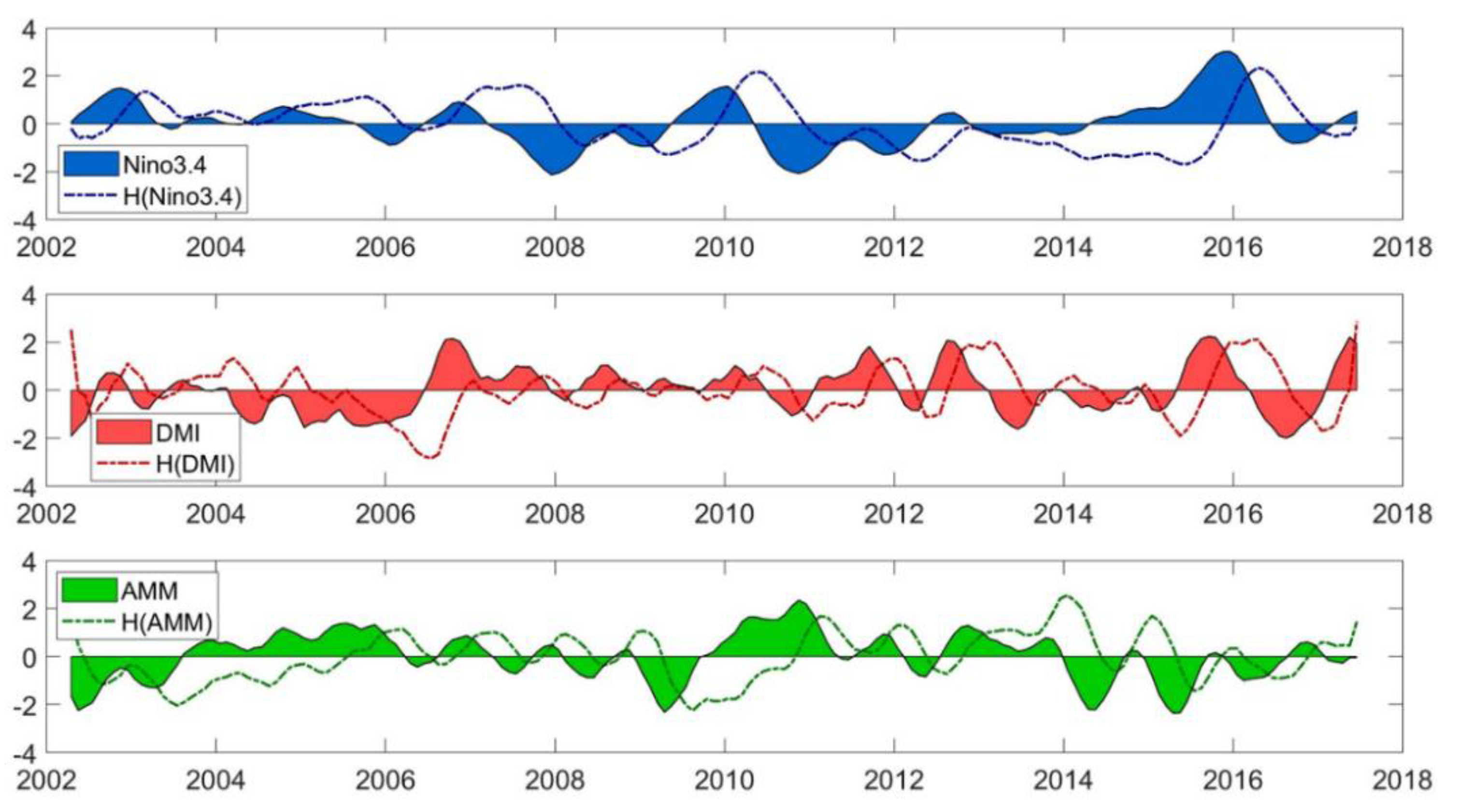
where (i, j) is the geographic location of grid cell, t is the time in years, a1 to a12 are the fitting coefficients, N(t), D(t) and A(t) are the normalized Niño 3.4, DMI and AMM indices, and ε(t) is residual error. These climate indices are shifted by π/2 in the frequency domain with Hilbert transformation (, [39]) to capture the out of phase pattern of TWS changes driven by ENSO/IOD/AMM [24,40]. For example, if there is no phase lag between the Niño 3.4 index and TWS changes at a given location, a8 approaches zero. The time series of Niño 3.4, DMI, and AMM along with the corresponding Hilbert transformations are shown in Figure 1.
In Equation (1), the coefficients a1 to a12 can be determined using the least squares fit, where a1 is the constant term, a2 is the linear rate, and a3 and a4 represent the annual amplitudes for the sine and cosine components, while the semi-annual signals are described by a5 and a6. Interannual TWS variations (TWSinter) can be computed as the residuals after removing the linear trend, annual, and semiannual cycles in Equation (1) and smoothing with a 5-month running mean:
The coefficients a7 and a8 in Equation (1) represent the TWS changes affected by ENSO; the variabilities due to IOD are described by a9 and a10, and that of AMM by a11 and a12. We calculate the corresponding amplitudes of TWS changes associated with these climate indices using these coefficients (a7 to a12) via Equations (3)–(5). The amplitude represents estimated magnitude of the influence of each of the three climate indices (i.e., contribution of a given climate index to TWS changes).
The TWS changes associated with ENSO, IOD, and AMM climate indices (hereafter called climate-induced TWS changes, and noted by subscript climate) can be computed from:
Here we use the root mean square (RMS) reduction [41] to investigate the degree of agreement between TWSinter and TWSclimate:
4. Results
4.1. ENSO/IOD/AMM Induced TWS Changes
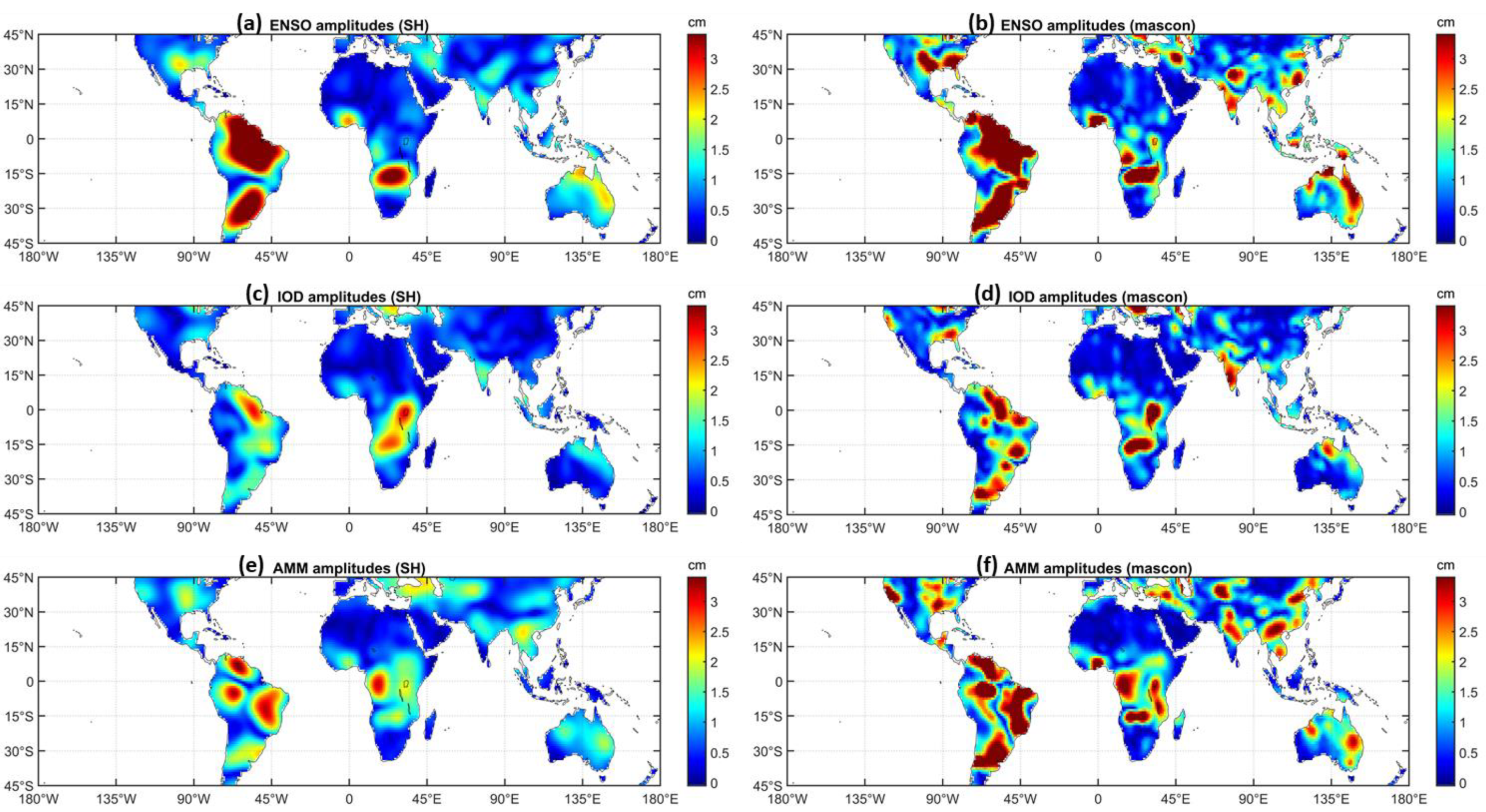
Using GRACE observations and three climate indices (i.e., Niño 3.4, DMI, and AMM indices), we obtain the fitting coefficients a1 to a12 in Equation (1), and then compute the ENSO/IOD/AMM amplitudes according to Equations (3)–(5). Figure 2 shows the ENSO/IOD/AMM amplitudes from the GRACE SH and mascon solutions, illustrating the possible connections of these climate phenomena with TWS changes. In each grid cell, the amplitude represents quantitative contribution of each phenomenon to the observed TWS changes (i.e., the larger the amplitude, the greater the contribution). For the GRACE SH solutions, the maximum ENSO/IOD/AMM amplitudes in global grid cells are ~11.1 cm, ~4.3 cm, ~4.4 cm, respectively; while ~27.5 cm, ~11.5 cm, and ~15.2 cm for the GRACE mascon solutions. In Figure 2, despite the amplitudes of mascon solutions show relatively higher spatial resolution and larger signal magnitudes, the spatial patterns of two GRACE solutions generally agree well at global scale. The differences in the signal magnitudes are mainly attributed to the leakage errors in the GRACE SH solutions, which are caused by both the truncation of SH coefficients and the 300 km Gaussian filter applied.
The significant influence of ENSO/IOD/AMM on TWS changes in the tropics and subtropics is clearly reflected in the relatively large amplitudes (e.g., greater than ~3 cm) shown in Figure 2. The spatial patterns of ENSO/IOD/AMM amplitudes indicate that ENSO, IOD, and AMM are three important climate factors affecting the TWS changes in South America, southeast region of North America, central Africa, southern Asia, and northern Australia. The contributions of each climate phenomenon to TWS changes in different regions vary substantially, and different climate indices show significantly different impacts on TWS changes. In most parts of the tropics and subtropics, the ENSO contribution to TWS changes is found to be more dominant than IOD and AMM. Additionally, due to the low water storage (and thus small fluctuations in water storage) in the Sahara Desert, the amplitudes in northern Africa are relatively small (close to zero).
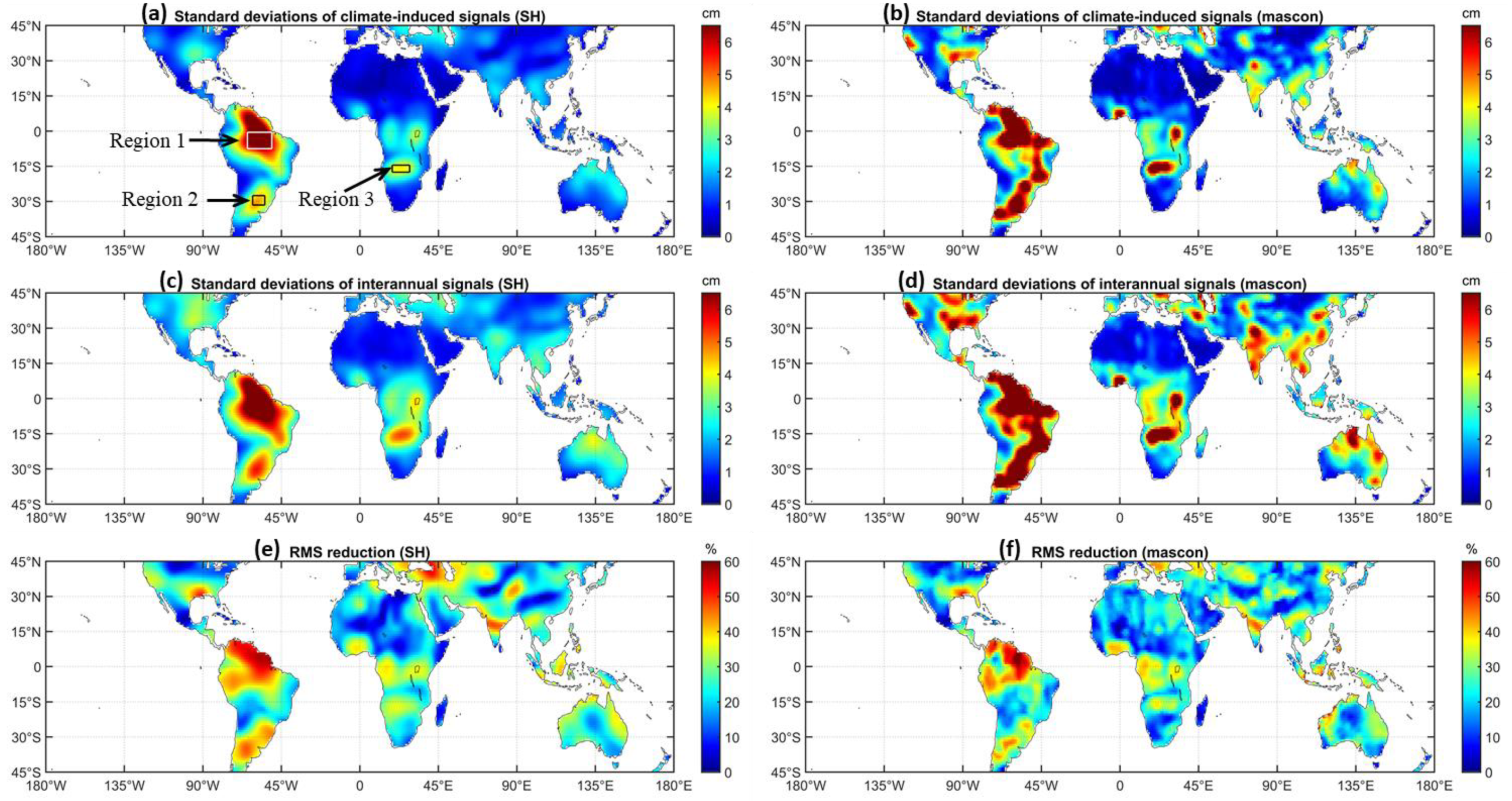
At interannual time scales, TWS changes in the tropics and subtropics are strongly influenced by ENSO, IOD, and AMM. Therefore, in this study, we compare climate-induced TWS changes (defined in Equation (6)) and interannual TWS changes to investigate the total contributions of ENSO, IOD, and AMM climate phenomena. Figure 3a–d show the comparisons between climate-induced TWS changes and interannual TWS changes from GRACE SH and mascon solutions. The standard deviations for Figure 3a–d are in the range of 0.2–11.8 cm, 0.1–27.6 cm, 0.6–12.8 cm, and 0.4–33.7 cm, respectively, further indicating the larger signal magnitudes in mascon solutions compared to SH solutions. The spatial patterns of climate-induced TWS changes and interannual TWS changes are generally in good agreement, while in most cases, the signal magnitudes of the former are significantly smaller than the latter.
In order to approximately quantify the degree of agreement between climate-induced TWS changes and interannual TWS changes, we compute the RMS reductions according to Equation (7), and the results are shown in Figure 3e,f. The percentages of RMS reduction are in the range of 0–60%, with the maximum located in the Amazon basin. Larger RMS reduction values indicate better agreement. Therefore, the areas with larger interannual TWS changes exhibit larger RMS reduction values, which suggests that climate-induced TWS changes and interannual TWS changes in these regions are in better agreement. In addition, the highly consistence (correlation coefficients ~0.90) of RMS reductions for the two GRACE solutions could verify the reliability of fitted results.
4.2. Correlation Analysis between TWS Changes and ENSO
The fitting coefficients a7 to a12 in Equation (1) not only provide quantifications of ENSO/IOD/AMM contributions to TWS changes, but also represent the connections between interannual TWS changes and these climate phenomena. To better understand the meaning of these fitting coefficients, we take coefficients a7 and a8 as examples to illustrate the possible correlation between TWS changes and ENSO.
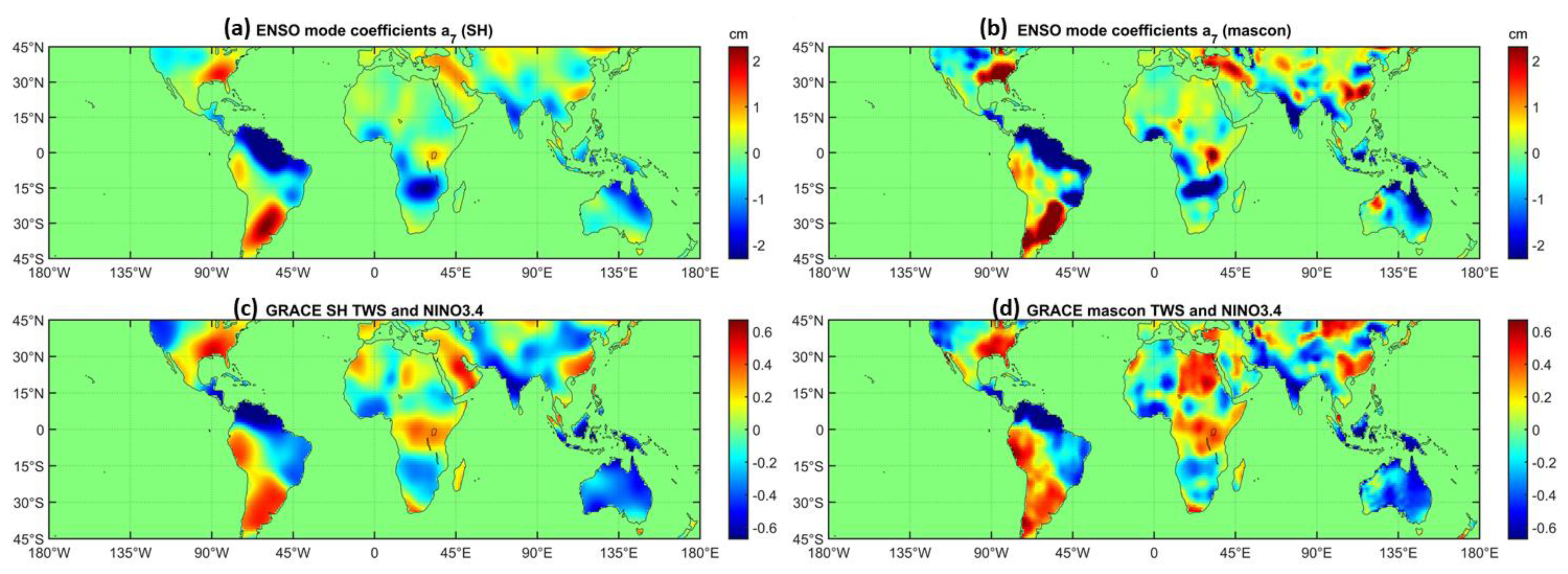
In Equation (1), a7 is the least squares fitting coefficient for normalized Niño 3.4 index. Figure 4 shows spatial distribution of coefficients a7 and cross correlation coefficients between interannual TWS changes and Niño 3.4 index for GRACE SH (left two panels) and mascon solutions (right two panels). The spatial patterns of coefficients a7 presented in Figure 4a,b generally agree well with those of GRACE-ENSO correlation in Figure 4c,d, while in northern Africa, the absolute value of a7 is relatively small. This is mainly because the northern Africa is mostly covered by deserts with low water storage. Therefore, to a certain extent, the coefficients a7 are “equivalent” to the cross correlations (without lag) between interannual TWS changes and Niño 3.4 index. Results indicate that the interannual TWS changes in most tropical and subtropical regions are strongly connected with ENSO. In addition, the good agreement of spatial patterns in Figure 4a–d also validates the least squares fitting results.
In Equation (1), a8 represents the fitting coefficients for Hilbert transformation of normalized Niño 3.4 index (i.e., N(t)). The Hilbert transformation of N(t) is given by:
This means that Hilbert transformed time series is related to the time integral of Niño 3.4 index. Therefore, coefficients a8 could reflect the connection between TWS changes and the time integral of Niño 3.4 index.
Based on the principle of water balance, TWS changes (ΔTWS) over a time period (Δt) reflect the sum of precipitation (P), evapotranspiration (E) and runoff (R) as:
ENSO events are characterized by anomalous SST and trade wind changes in the tropical Pacific, which could significantly impact the energy exchange and moisture advection, and might eventually cause precipitation anomalies in different areas around the globe [14]. Therefore, Equation (9) suggests that the time derivative of TWS changes (i.e., TWS flux) is expected to connect with ENSO. At global 1° × 1°grid, we compute monthly TWS flux as the quantitative difference of TWS changes between two adjacent months, and then apply the usual data processing method to obtain the interannual TWS flux. Finally, we analyze the relationship of interannual TWS flux and Niño 3.4 index.
Figure 5 shows the least squares fitting coefficients a8 and the zero-phase-lag cross correlation coefficients between interannual TWS flux and Niño 3.4 index. The spatial patterns of coefficients a8 presented in Figure 5a,b are similar to those of GRACE-ENSO correlation in Figure 5c,d. This is reasonable, considering if TWS flux is related to Niño 3.4 index, and then TWS changes, which means the integral of TWS flux over time, might be correlated with the time integral of Niño 3.4 index. Therefore, the coefficients a8 could reflect the correlation between interannual TWS flux and Niño 3.4 index. It is interesting to note that in many parts of the world, the ENSO coefficients a7 and a8 show substantially different spatial patterns (e.g., Figure 4a and Figure 5a), and the coefficients a8 appear to show more pronounced and spatially correlated patterns (e.g., in the broad Amazon basin). The TWS flux also shows notably stronger cross correlation with Niño 3.4 index in certain regions (e.g., Amazon and La Plata basins). This illustrates the closer connections between TWS flux changes and precipitation anomalies tied to the ENSO events in related regions.
4.3. Regional Analysis
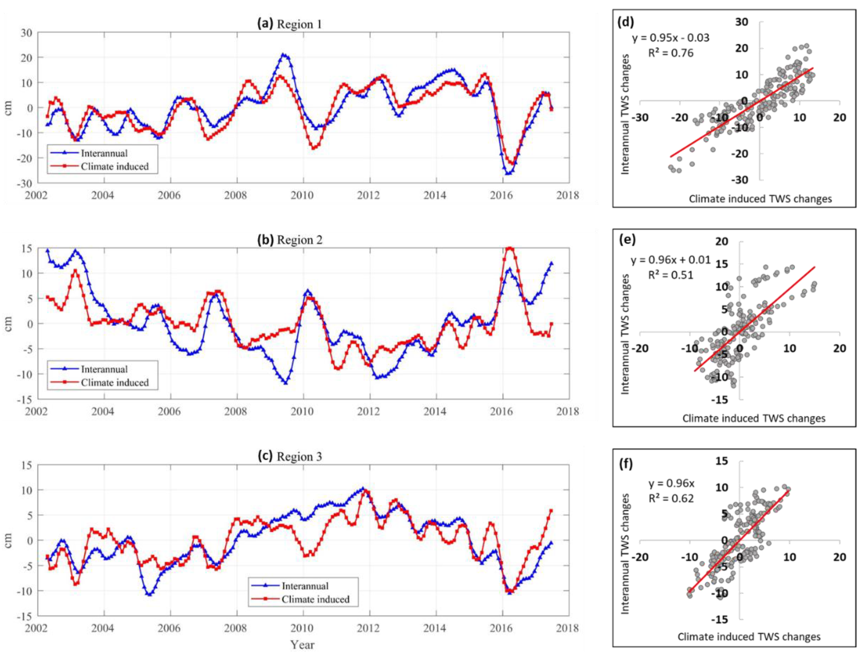
In Section 4.1, the contributions of ENSO/IOD/AMM to interannual TWS changes have been discussed in the spatial domain. To investigate the degree of agreement between climate-induced TWS changes and interannual TWS changes in the time domain, three regions (circled by the white/black boxes in Figure 3a) are selected for further analysis. Figure 6 shows the time series of both interannual and climate-induced TWS changes and their linear relationship in these regions, and the related statistics are summarized in Table 1. Here, we only provide the results computed from SH solutions, and mascon solutions were also used for computation and showed similar results (not shown in this study). The good agreements among signals in Figure 6 suggest that interannual TWS changes of these regions are strongly influenced by ENSO, IOD, and AMM. Additionally, the dominant contribution of ENSO to interannual TWS changes is clearly reflected in the larger amplitudes in Table 1.
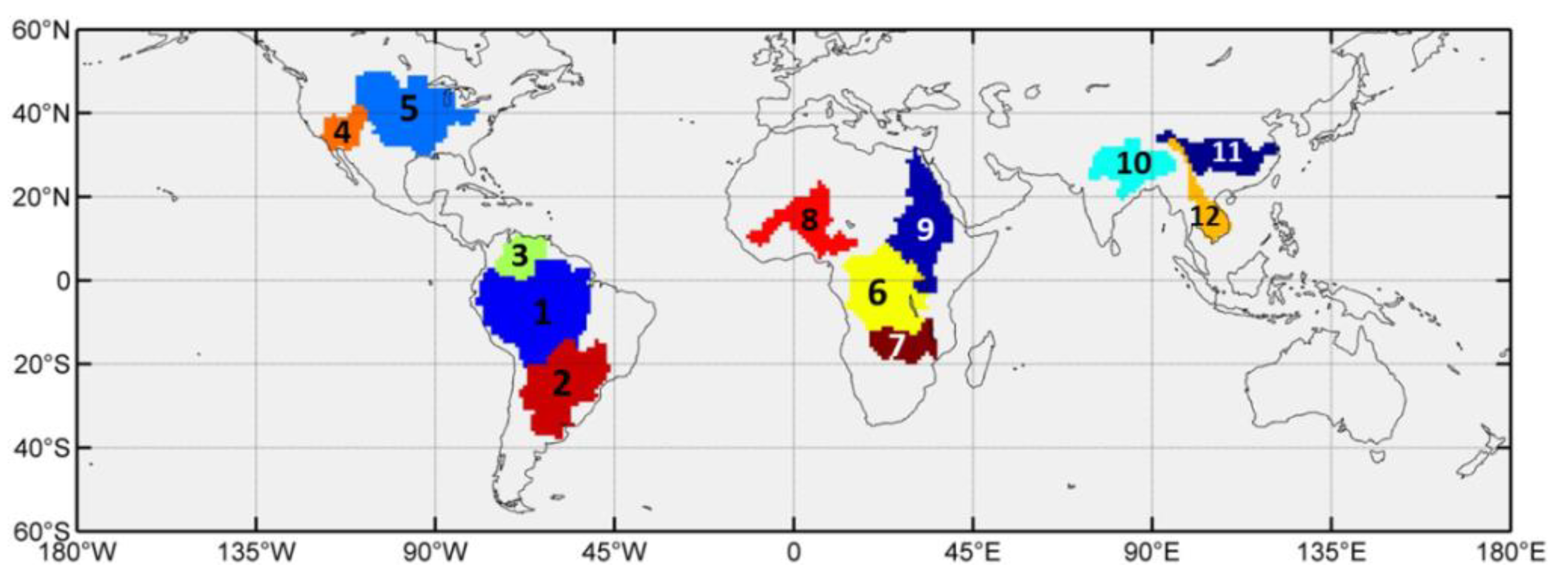
Due to the special hydro-climatic and economical importance of river basins, several major river basins in the tropics and subtropics are also selected for similar analysis. The geographic locations of these river basins are shown in Figure 7, and the statistics about interannual and climate-induced TWS changes are summarized in Table 2. Similar to the spatial patterns in Figure 2, the contribution of each climate phenomenon to TWS changes might vary in different river basins. For example, the ENSO contribution to TWS changes is likely more dominant than those from IOD and AMM in the Amazon, La Plata, Orinoco, Zambezi, and Ganges River basins. The AMM amplitudes in the Mississippi, Congo, Nile and Mekong basins are larger than those of ENSO and IOD. Despite the different contributions of these climate phenomena, the total contributions of ENSO/IOD/AMM to interannual TWS changes in these basins are clearly significant (with maximum percentages up to ~90%).
5. Discussions
The focus of this study is to investigate the connections between interannual TWS changes and ENSO/IOD/AMM climate indices, which relies on the assumption that these climate indices are linearly independent:
- (a)
- According to Saji et al. (1999) [36], IOD is inherent and unique in the Indian Ocean, and is likely to be independent of ENSO in the Pacific Ocean. They have demonstrated that the relationship between DMI and Niño 3 SST anomaly is weak (<0.35). Similarly, we also computed the correlation coefficient between DMI and Niño 3.4 index used in this study, and found their correlation is also quite weak (~0.27). Therefore, we could conclude that ENSO and IOD climate indices are mostly linearly independent.
- (b)
- According to the definition of AMM index, a commonly used ENSO index (cold tongue index averaged over 6° S–6° N and 180°–90° W) has been removed from all fields before the calculation of AMM time series [38]. Thus, the AMM index represents the dominant mode of non-ENSO coupled ocean–atmosphere variability in the tropical Atlantic. Furthermore, the correlation between AMM index and Niño 3.4 index used in the study is not significant (−0.28). Therefore, AMM index is considered as independent of ENSO index.
- (c)
- The correlation coefficient between DMI and AMM index approximately equals to zero, which suggests that IOD and AMM climate indices are also independent.
In summary, ENSO/IOD/AMM climate indices are linearly independent of each other. Therefore, to some extent, the fitting coefficients a7 to a12 obtained from Equation (1) would not influence each other too much. That is to say, the fitting results of Equation (1) are reasonable and interpretable.
The ENSO/IOD/AMM amplitudes in Figure 2 are relatively significant (generally greater than ~3 cm), indicating ENSO, IOD, and AMM are important climate factors affecting TWS changes in the tropics and subtropics. However, the contribution of each climate phenomenon to TWS changes might vary in different regions. For example, the ENSO contribution to TWS changes is found to be more dominant than IOD and AMM in the Amazon, Orinoco, and La Plata River basins of South America. This is likely due to that these basins are close to tropical Pacific, where abnormal SSTs and trade wind changes associated with ENSO events would significantly influence the moisture exchange with neighboring continent. In addition, the AMM amplitudes in the Mississippi, Congo, Nile, and Mekong basins are larger than those of ENSO and IOD. Therefore, the amplitude analyses are helpful to identify regions over the world where interannual TWS changes are closely related to ENSO, IOD, and AMM, and which kind of climate variability plays the leading role.
According to Equation (6), we quantify the total contributions of ENSO/IOD/AMM to interannual TWS changes in the tropics and subtropics (Figure 3). The spatial patterns of climate-induced TWS changes and interannual TWS changes are generally in good agreement. The climate-induced TWS changes are especially significant in the tropics such as northern South America and central Africa. The climate variability in the above regions is mainly driven by the seasonal and interannual migrations of ITCZ, resulting in significant precipitation anomalies related to ENSO, IOD, and AMM.
As we mentioned in Section 3, different phases of ENSO/IOD/AMM might affect TWS changes. Therefore, the time lag information has important implications for monitoring water storage response to climate variability and predicting global and regional TWS changes. For example, in a region with large ENSO amplitudes like the Amazon basin, if ENSO events occur before TWS anomalies for several months, the typical phase shift (when climate variability leads TWS changes) can be used to forecast major drought and flood events.
It should be pointed out that there are numerous factors impacting GRACE TWS estimates and the computation results in this study. The spatial filters applied in GRACE SH solutions are considered to have removed the most of small-scale signals, and have reduced the magnitudes of TWS changes at the same time. Residual errors in GRACE observations and uncertainty in low-degree SH coefficients also influence the computation results. Since the focus of this study is to analyze the relative contributions of ENSO, IOD and AMM to TWS changes at global and large regional scales, the attenuation effect in GRACE estimates would not significantly impact the results, which can be proved by the comparisons of similar results from GRACE SH and GRACE mascon solutions in Figure 2, Figure 3, Figure 4 and Figure 5. Furthermore, the main interest in this study is to analyze TWS changes at relatively large scales, so lack of small-scale signals should not influence the main conclusions.
Several previous studies have analyzed the impact of large-scale ocean–atmosphere interactions on TWS changes. These studies mainly carried out regional analysis, with few focused on global scales. In recent years, a few studies investigated the influence of ENSO on global TWS changes (e.g., [14,24,25]). However, ENSO is mainly based on SST variability in the tropical Pacific, contributions of other large-scale ocean–atmosphere interactions from the Indian and Atlantic Oceans should also be taken into account. In this study, we mainly investigate the impact of ENSO, IOD, and AMM on interannual TWS changes. However, anthropogenic activities (e.g., groundwater pumping for irrigation and domestic consumption) might also impact water storage changes in many parts of the world (e.g., [5,42,43,44]). Therefore, a more comprehensive analysis would consider the anthropogenic influence, which is beyond the scope of the present study.
6. Conclusions
This study provides a comprehensive investigation of connections between interannual TWS changes in the tropics and subtropics and large-scale climate variability (i.e., ENSO, IOD, and AMM) in the Pacific, Indian, and Atlantic Oceans. GRACE measurements and three climate indices (i.e., Niño 3.4, DMI and AMM indices) are used to explore the impacts of ENSO, IOD, and AMM on interannual TWS changes in the tropics and subtropics. Based on the least square principle, these climate indices, and the corresponding Hilbert transformations, together with a linear trend, annual, and semi-annual terms, are fitted to the TWS time series on global 1° × 1° grids. The fitting coefficients a7 to a12 can not only quantify contributions of ENSO/IOD/AMM to TWS changes, but also represent connections of interannual TWS changes with these climate phenomena. In this study, we take the ENSO coefficients a7 and a8 as examples to illustrate the possible correlation between TWS changes and ENSO. To a certain extent, the ENSO coefficients a7 are equivalent to the cross correlations (without lag) between interannual TWS changes and Niño 3.4 index, and coefficients a8 reflect the correlations between interannual TWS flux and Niño 3.4 index.
Using the fitting coefficients, we compute the ENSO/IOD/AMM amplitudes from GRACE SH and mascon solutions. The spatial patterns of two GRACE solutions generally agree well, whereas the amplitudes of mascon solutions have relatively higher spatial resolution and larger signal magnitudes. At interannual time scales, TWS changes in the tropics and subtropics are strongly affected by ENSO, IOD, and AMM. The contribution of each climate phenomenon to TWS changes might vary in different regions, while in most parts of the tropics and subtropics, ENSO contribution to TWS changes is found to be more dominant than those from IOD and AMM. In addition, the total contribution of ENSO/IOD/AMM to interannual TWS changes is clearly more significant (with maximum percentages up to ~90%), than individual contributions from these climate phenomena. The climate-induced TWS changes and interannual TWS changes generally agree well at both temporal and spatial scales, indicating that interannual TWS changes in the tropics and subtropics are significantly correlated with ENSO, IOD, and AMM.
Author Contributions
S.N. carried out the research and wrote the original manuscript. Z.L. and J.C. contributed to the preparation of the manuscript through reviews and comments. J.L. contributed to the discussion of the results. All authors have read and agreed to the published version of the manuscript.
Funding
This study was funded by the National Key R&D Program of China (2018YFC1503503), the National Natural Science Foundation of China (42004017, 42061134007, 42074018, 11873075), the China Postdoctoral Science Foundation (2018M642847), and the Natural Science Foundation of Shanghai (20ZR1467400).
Data Availability Statement
The data presented in this research are available upon request from the corresponding authors.
Conflicts of Interest
The authors declare no conflict of interest.
References
- Llovel, W.; Becker, M.; Cazenave, A.; Crétaux, J.-F.; Ramillien, G. Global land water storage change from GRACE over 2002–2009; Inference on sea level. C. R. Geosci. 2010, 342, 179–188. [Google Scholar] [CrossRef]
- Tapley, B.D.; Bettadpur, S.; Ries, J.C.; Thompson, P.F.; Watkins, M.M. GRACE measurements of mass variability in the Earth system. Science 2004, 305, 503–505. [Google Scholar] [CrossRef] [Green Version]
- Wahr, J.; Swenson, S.; Zlotnicki, V.; Velicogna, I. Time-variable gravity from GRACE: First results. Geophys. Res. Lett. 2004, 31, L11501. [Google Scholar] [CrossRef] [Green Version]
- Crowley, J.W.; Mitrovica, J.X.; Bailey, R.C.; Tamisiea, M.E.; Davis, J.L. Land water storage within the Congo Basin inferred from GRACE satellite gravity data. Geophys. Res. Lett. 2006, 33. [Google Scholar] [CrossRef]
- Rodell, M.; Velicogna, I.; Famiglietti, J.S. Satellite-based estimates of groundwater depletion in India. Nature 2009, 460, 999–1002. [Google Scholar] [CrossRef] [Green Version]
- Ni, S.; Chen, J.; Wilson, C.R.; Hu, X. Long-term water storage changes of Lake Volta from GRACE and satellite altimetry and connections with regional climate. Remote Sens. 2017, 9, 842. [Google Scholar] [CrossRef] [Green Version]
- Zhou, H.; Zhou, Z.; Luo, Z. A new hybrid processing strategy to improve temporal gravity field solution. J. Geophys. Res. Solid Earth 2019, 124, 9415–9432. [Google Scholar] [CrossRef]
- Leblanc, M.J.; Tregoning, P.; Ramillien, G.; Tweed, S.O.; Fakes, A. Basin-scale, integrated observations of the early 21st century multiyear drought in southeast Australia. Water Resour. Res. 2009, 45, 546–550. [Google Scholar] [CrossRef]
- Chen, J.L.; Wilson, C.R.; Tapley, B.D.; Longuevergne, L.; Yang, Z.L.; Scanlon, B.R. Recent La Plata basin drought conditions observed by satellite gravimetry. J. Geophys. Res. Atmos. 2010, 115. [Google Scholar] [CrossRef]
- Abelen, S.; Seitz, F.; Abarca-del-Rio, R.; Güntner, A. Droughts and floods in the La Plata Basin in soil moisture data and GRACE. Remote Sens. 2015, 7, 7324–7349. [Google Scholar] [CrossRef] [Green Version]
- García-García, D.; Ummenhofer, C.C.; Zlotnicki, V. Australian water mass variations from GRACE data linked to Indo-Pacific climate variability. Remote Sens. Environ. 2011, 115, 2175–2183. [Google Scholar] [CrossRef] [Green Version]
- De Linage, C.; Kim, H.; Famiglietti, J.S.; Yu, J.-Y. Impact of Pacific and Atlantic sea surface temperatures on interannual and decadal variations of GRACE land water storage in tropical South America. J. Geophys. Res. Atmos. 2013, 118, 10811–10829. [Google Scholar] [CrossRef] [Green Version]
- Ndehedehe, C.E.; Awange, J.L.; Kuhn, M.; Agutu, N.O.; Fukuda, Y. Climate teleconnections influence on West Africa’s terrestrial water storage. Hydrol. Process. 2017, 31, 3206–3224. [Google Scholar] [CrossRef] [Green Version]
- Ni, S.; Chen, J.; Wilson, C.R.; Li, J.; Hu, X.; Fu, R. Global terrestrial water storage changes and connections to ENSO events. Surv. Geophys. 2018, 39, 1–22. [Google Scholar] [CrossRef]
- Syed, T.H.; Famiglietti, J.S.; Rodell, M.; Chen, J.L.; Wilson, C.R. Analysis of terrestrial water storage changes from GRACE and GLDAS. Water Resour. Res. 2008, 44, W02433. [Google Scholar] [CrossRef]
- Crowley, J.W.; Mitrovica, J.X.; Bailey, R.C.; Tamisiea, M.E.; Davis, J.L. Annual variations in water storage and precipitation in the Amazon Basin. J. Geod. 2008, 82, 9–13. [Google Scholar] [CrossRef]
- Nie, N.; Zhang, W.; Guo, H.; Ishwaran, N. 2010-2012 drought and flood events in the Amazon Basin inferred by GRACE satellite observations. J. Appl. Remote Sens. 2015, 9, 096023. [Google Scholar] [CrossRef]
- Van Dijk, A.I.J.M.; Beck, H.E.; Crosbie, R.S.; de Jeu, R.A.M.; Liu, Y.Y.; Podger, G.M.; Timbal, B.; Viney, N.R. The Millennium Drought in southeast Australia (2001–2009): Natural and human causes and implications for water resources, ecosystems, economy, and society. Water Resour. Res. 2013, 49, 1040–1057. [Google Scholar] [CrossRef]
- Forootan, E.; Safari, A.; Mostafaie, A.; Schumacher, M.; Delavar, M.; Awange, J.L. Large-scale total water storage and water fux changes over the arid and semiarid parts of the Middle East from GRACE and reanalysis products. Surv. Geophys. 2017, 38, 591–615. [Google Scholar] [CrossRef] [Green Version]
- Tang, J.; Cheng, H.; Liu, L. Assessing the recent droughts in Southwestern China using satellite gravimetry. Water Resour. Res. 2014, 50, 3030–3038. [Google Scholar] [CrossRef]
- Thomas, A.C.; Reager, J.T.; Famiglietti, J.S.; Rodell, M. A GRACE-based water storage deficit approach for hydrological drought characterization. Geophys. Res. Lett. 2014, 41, 1537–1545. [Google Scholar] [CrossRef] [Green Version]
- Xiao, M.; Koppa, A.; Mekonnen, Z.; Pagán, B.R.; Zhan, S.; Cao, Q.; Aierken, A.; Lee, H.; Lettenmaier, D.P. How much groundwater did California’s Central Valley lose during the 2012-2016 drought? Geophys. Res. Lett. 2017, 44, 4872–4879. [Google Scholar] [CrossRef]
- Anyah, R.O.; Forootan, E.; Awange, J.L.; Khaki, M. Understanding linkages between global climate indices and terrestrial water storage changes over Africa using GRACE products. Sci. Total Environ. 2018, 635, 1405–1416. [Google Scholar] [CrossRef] [PubMed] [Green Version]
- Phillips, T.; Nerem, R.S.; Fox-Kemper, B.; Famiglietti, J.S.; Rajagopalan, B. The influence of ENSO on global terrestrial water storage using GRACE. Geophys. Res. Lett. 2012, 39, L16705. [Google Scholar] [CrossRef] [Green Version]
- Eicker, A.; Forootan, E.; Springer, A.; Longuevergne, L.; Kusche, J. Does GRACE see the terrestrial water cycle “intensifying”? J. Geophys. Res. Atmos. 2016, 121, 733–745. [Google Scholar] [CrossRef] [Green Version]
- Peltier, W.R.; Argus, D.F.; Drummond, R. Comment on “An Assessment of the ICE-6G_C (VM5a) Glacial Isostatic Adjustment Model” by Purcell et al. J. Geophys. Res. Solid Earth 2018, 123, 2019–2028. [Google Scholar] [CrossRef]
- Cheng, M.; Ries, J. The unexpected signal in GRACE estimates of C20. J. Geod. 2017, 91, 897–914. [Google Scholar] [CrossRef]
- Sun, Y.; Riva, R.; Ditmar, P. Optimizing estimates of annual variations and trends in geocenter motion and J2 from a combination of GRACE data and geophysical models. J. Geophys. Res. Solid Earth 2016, 121, 8352–8370. [Google Scholar] [CrossRef] [Green Version]
- Swenson, S.; Wahr, J. Post-processing removal of correlated errors in GRACE data. Geophys. Res. Lett. 2006, 33. [Google Scholar] [CrossRef]
- Jekeli, C. Alternative Methods to Smooth the Earth’s Gravity Field; Department of Geodetic Science and Surveying, Ohio State University: Columbus, OH, USA, 1981. [Google Scholar]
- Wahr, J.; Molenaar, M.; Bryan, F. Time variability of the Earth’s gravity field: Hydrological and oceanic effects and their possible detection using GRACE. J. Geophys. Res. Solid Earth 1998, 103, 30205–30229. [Google Scholar] [CrossRef]
- Save, H.; Bettadpur, S.; Tapley, B.D. High-resolution CSR GRACE RL05 mascons. J. Geophys. Res. Solid Earth 2016, 121, 7547–7569. [Google Scholar] [CrossRef]
- Watkins, M.M.; Wiese, D.N.; Yuan, D.-N.; Boening, C.; Landerer, F.W. Improved methods for observing Earth’s time variable mass distribution with GRACE using spherical cap mascons. J. Geophys. Res. Solid Earth 2015, 120, 2648–2671. [Google Scholar] [CrossRef]
- Trenberth, K.E.; Caron, J.M.; Stepaniak, D.P.; Worley, S. Evolution of El Niño-Southern Oscillation and global atmospheric surface temperatures. J. Geophys. Res. Atmos. 2002, 107, AAC 5-1–AAC 5-7. [Google Scholar] [CrossRef]
- Trenberth, K.E. The definition of El Niño. Bull. Am. Meteorol. Soc. 1997, 78, 2771–2777. [Google Scholar] [CrossRef] [Green Version]
- Saji, N.; Goswami, B.; Vinayachandran, P.; Yamagata, T. A dipole mode in the tropical Indian Ocean. Nature 1999, 401, 360–363. [Google Scholar] [CrossRef] [PubMed]
- Foltz, G.R.; McPhaden, M.J. Interaction between the Atlantic meridional and Niño modes. Geophys. Res. Lett. 2010, 37. [Google Scholar] [CrossRef] [Green Version]
- Chiang, J.C.H.; Vimont, D.J. Analogous Pacific and Atlantic Meridional Modes of Tropical Atmosphere–Ocean Variability*. J. Clim. 2004, 17, 4143–4158. [Google Scholar] [CrossRef]
- Horel, J.D. Complex principal component analysis: Theory and examples. J. Clim. Appl. Meteorol. 1984, 23, 1660–1673. [Google Scholar] [CrossRef]
- Forootan, E.; Awange, J.; Schumacher, M.; Anyah, R.; van Dijk, A.; Kusche, J. Quantifying the impacts of ENSO and IOD on rain gauge and remotely sensed precipitation products over Australia. Remote Sens. Environ. 2016, 172, 50–66. [Google Scholar] [CrossRef] [Green Version]
- Van Dam, T.; Wahr, J.; Lavallée, D. A comparison of annual vertical crustal displacements from GPS and Gravity Recovery and Climate Experiment (GRACE) over Europe. J. Geophys. Res. Solid Earth 2007, 112, B03404. [Google Scholar] [CrossRef] [Green Version]
- Ahmed, M.; Sultan, M.; Wahr, J.; Yan, E. The use of GRACE data to monitor natural and anthropogenic induced variations in water availability across Africa. Earth Sci. Rev. 2014, 136, 289–300. [Google Scholar] [CrossRef]
- Pokhrel, Y.N.; Koirala, S.; Yeh, P.J.F.; Hanasaki, N.; Longuevergne, L.; Kanae, S.; Oki, T. Incorporation of groundwater pumping in a global Land Surface Model with the representation of human impacts. Water Resour. Res. 2015, 51, 78–96. [Google Scholar] [CrossRef] [Green Version]
- Chen, J.L.; Wilson, C.R.; Tapley, B.D.; Scanlon, B.; Güntner, A. Long-term groundwater storage change in Victoria, Australia from satellite gravity and in situ observations. Glob. Planet. Chang. 2016, 139, 56–65. [Google Scholar] [CrossRef] [Green Version]
Figure 1.
ENSO, IOD, and AMM indices and the corresponding Hilbert transformed time series.

Figure 2.
ENSO, IOD, and AMM amplitudes from GRACE spherical harmonics (SH) and mascon solutions. (a,b) show ENSO amplitudes from GRACE SH and mascon solutions computed with Equation (3); (c,d) show IOD amplitudes from GRACE SH and mascon solutions computed with Equation (4); (e,f) show AMM amplitudes from GRACE SH and mascon solutions computed with Equation (5).

Figure 3.
Comparisons between climate-induced TWS changes defined in Equation (6) and interannual TWS changes: (a,b) standard deviations of climate-induced TWS changes from GRACE SH and mascon solutions, (c,d) standard deviations of interannual TWS changes from GRACE SH and mascon solutions, and (e,f) RMS reductions between climate-induced TWS changes and interannual TWS changes from GRACE SH and mascon solutions.

Figure 4.
ENSO coefficients a7 of least squares fitting and zero-phase-lag cross correlation coefficients between interannual TWS changes and Niño 3.4 index. (a,b) show ENSO coefficients a7 obtained from GRACE SH and mascon solutions, respectively; (c) shows correlation coefficients between TWS changes from GRACE SH solutions and Niño 3.4 index; and (d) shows the cross-correlation coefficients between TWS changes from GRACE mascon solutions and Niño 3.4 index.

Figure 5.
The same as Figure 4, but for ENSO coefficients, a8 and cross correlation coefficients between interannual TWS flux and Niño 3.4 index. It should be noted that the TWS flux in this study means the quantitative difference of TWS changes between two adjacent months.
Figure 5.
The same as Figure 4, but for ENSO coefficients, a8 and cross correlation coefficients between interannual TWS flux and Niño 3.4 index. It should be noted that the TWS flux in this study means the quantitative difference of TWS changes between two adjacent months.

Figure 6.
The interannual and climate induced TWS changes from GRACE SH solutions in the three selected regions shown in Figure 3a. (a–c) show the interannual TWS changes (blue curves) and climate induced TWS changes (red curves) for Regions 1–3. (d–f) show the corresponding linear fitting relationship between the two curves in the three regions.

Figure 7.
Selected major river basins in the tropics and subtropics (1—Amazon, 2—La Plata, 3—Orinoco, 4—Colorado, 5—Mississippi, 6—Congo, 7—Zambezi, 8—Niger, 9—Nile, 10—Ganges, 11—Yangtze, 12—Mekong).
Figure 7.
Selected major river basins in the tropics and subtropics (1—Amazon, 2—La Plata, 3—Orinoco, 4—Colorado, 5—Mississippi, 6—Congo, 7—Zambezi, 8—Niger, 9—Nile, 10—Ganges, 11—Yangtze, 12—Mekong).


Table 1.
Statistics of interannual and climate-induced TWS changes in the three selected regions.
| Regions | Standard Deviations/cm | Coefficients of Determination 1 | Amplitudes/cm | |||
|---|---|---|---|---|---|---|
| Interannual | Climate Induced | ENSO | IOD | AMM | ||
| Region 1 | 9.00 | 8.24 | 0.76 | 8.05 | 1.48 | 0.97 |
| Region 2 | 6.26 | 4.70 | 0.51 | 4.65 | 0.81 | 2.26 |
| Region 3 | 5.12 | 4.25 | 0.62 | 4.20 | 2.43 | 1.82 |
Table 2.
Statistics of interannual and climate-induced TWS changes for selected major river basins.
| River Basins | Standard Deviations/cm | Coefficients of Determination | Amplitudes/cm | |||
|---|---|---|---|---|---|---|
| Interannual | Climate Induced | ENSO | IOD | AMM | ||
| Amazon | 4.70 | 4.29 | 0.75 | 3.87 | 0.50 | 0.79 |
| La Plata | 2.95 | 2.35 | 0.47 | 2.11 | 0.33 | 0.81 |
| Orinoco | 4.65 | 4.20 | 0.75 | 2.95 | 1.09 | 1.97 |
| Colorado | 2.58 | 1.94 | 0.52 | 0.76 | 1.29 | 1.22 |
| Mississippi | 2.89 | 1.58 | 0.27 | 0.48 | 0.36 | 1.36 |
| Congo | 2.62 | 2.02 | 0.53 | 0.87 | 1.45 | 1.86 |
| Zambezi | 3.95 | 2.95 | 0.59 | 2.89 | 2.01 | 1.29 |
| Niger | 1.21 | 0.71 | 0.31 | 0.56 | 0.36 | 0.42 |
| Nile | 1.52 | 1.11 | 0.35 | 0.57 | 0.16 | 1.00 |
| Ganges | 2.37 | 1.55 | 0.39 | 0.96 | 0.27 | 0.85 |
| Yangtze | 1.53 | 0.77 | 0.22 | 0.51 | 0.52 | 0.14 |
| Mekong | 2.61 | 1.52 | 0.30 | 0.58 | 0.36 | 1.29 |
Publisher’s Note: MDPI stays neutral with regard to jurisdictional claims in published maps and institutional affiliations. |
© 2021 by the authors. Licensee MDPI, Basel, Switzerland. This article is an open access article distributed under the terms and conditions of the Creative Commons Attribution (CC BY) license (https://creativecommons.org/licenses/by/4.0/).
Share and Cite
MDPI and ACS Style
Ni, S.; Luo, Z.; Chen, J.; Li, J. Impact of Large-Scale Ocean–Atmosphere Interactions on Interannual Water Storage Changes in the Tropics and Subtropics. Remote Sens. 2021, 13, 3529. https://0-doi-org.brum.beds.ac.uk/10.3390/rs13173529
AMA Style
Ni S, Luo Z, Chen J, Li J. Impact of Large-Scale Ocean–Atmosphere Interactions on Interannual Water Storage Changes in the Tropics and Subtropics. Remote Sensing. 2021; 13(17):3529. https://0-doi-org.brum.beds.ac.uk/10.3390/rs13173529
Chicago/Turabian StyleNi, Shengnan, Zhicai Luo, Jianli Chen, and Jin Li. 2021. "Impact of Large-Scale Ocean–Atmosphere Interactions on Interannual Water Storage Changes in the Tropics and Subtropics" Remote Sensing 13, no. 17: 3529. https://0-doi-org.brum.beds.ac.uk/10.3390/rs13173529
Note that from the first issue of 2016, this journal uses article numbers instead of page numbers. See further details here.