
Sentinel-2 Cloud Removal Considering Ground Changes by Fusing Multitemporal SAR and Optical Images

1
School of Geodesy and Geomatics, Wuhan University, Wuhan 430079, China
2
School of Sports Engineering and Information Technology, Wuhan Sports University, Wuhan 430079, China
3
Surveying and Mapping Science Institute of Zhejiang, Hangzhou 311100, China
*
Author to whom correspondence should be addressed.
†
Equal contribution.
Remote Sens. 2021, 13(19), 3998; https://0-doi-org.brum.beds.ac.uk/10.3390/rs13193998
Submission received: 27 July 2021
/
Revised: 23 September 2021
/
Accepted: 29 September 2021
/
Published: 7 October 2021
(This article belongs to the Section AI Remote Sensing)
Abstract
:Publicly available optical remote sensing images from platforms such as Sentinel-2 satellites contribute much to the Earth observation and research tasks. However, information loss caused by clouds largely decreases the availability of usable optical images so reconstructing the missing information is important. Existing reconstruction methods can hardly reflect the real-time information because they mainly make use of multitemporal optical images as reference. To capture the real-time information in the cloud removal process, Synthetic Aperture Radar (SAR) images can serve as the reference images due to the cloud penetrability of SAR imaging. Nevertheless, large datasets are necessary because existing SAR-based cloud removal methods depend on network training. In this paper, we integrate the merits of multitemporal optical images and SAR images to the cloud removal process, the results of which can reflect the ground information change, in a simple convolution neural network. Although the proposed method is based on deep neural network, it can directly operate on the target image without training datasets. We conduct several simulation and real data experiments of cloud removal in Sentinel-2 images with multitemporal Sentinel-1 SAR images and Sentinel-2 optical images. Experiment results show that the proposed method outperforms those state-of-the-art multitemporal-based methods and overcomes the constraint of datasets of those SAR-based methods.
1. Introduction
Remote sensing platforms such as Sentinel-2 satellites provide a large number of observation optical images, which contribute a lot to observation tasks such as Earth monitoring [1,2,3] and agriculture [4,5]. Nevertheless, the existence of cloud results in the severe information loss, which has a negative impact on the further application of remote sensing images. According to the statistics [6], above half of the Earth is covered by cloud so reconstruction of missing information caused by cloud is of great value. According to acquisition time of reference data in the reconstruction, traditional cloud removal can be classified into three families [7] which are, respectively, spatial-based methods, spectral-based methods and multitemporal-based methods.
Spectral-based methods make use of the bands with intact information as reference to reconstruct the bands’ missing information by establishing the relationship between bands. The reconstruction of dead pixels in Aqua MODIS band 6, where 15 of the 20 detectors are non-functional, is a classical case. Several spectral-based methods [8,9] solve this problem by establishing the polynomial models between bands. Generally, results of spectral-based methods are of high visual effect and accuracy, but they cannot deal with the situation where all bands have missing information. Spatial-based methods can deal with the missing information of all bands. They assume that the missing information and the remaining information share the same statistic law and geometrical structure so the missing information can be reconstructed from the remaining information. Spatial-based methods can be further sub-divided into four sub-classes, which are, respectively, interpolation methods [10,11], propagation diffusion methods [12,13,14], variation-based methods [15,16] and exemplar-based methods [17,18]. Spatial-based methods can well reconstruct the missing information of all bands, but they can only deal with the missing areas with small sizes. Even worse, the authority of reconstruction parts cannot be guaranteed because the reconstruction process is all based on the statistic of remaining areas. Multitemporal-based methods make use of homogeneous data from other times as reference to reconstruct the missing information. They outperform the above two methods in the reconstruction of large missing information. The precondition of traditional heterochronic methods is that there is no ground change occurring between the two periods. The multitemporal-based methods can be further divided into three sub-classes which are, respectively, replacement methods [19,20], learning methods [21,22] and filtering methods [23,24]. Recently, some multitemporal cloud removal methods based on deep learning have been proposed. For example, Uzkent, et al. [25] introduced deep neural network into the multitemporal cloud removal task, where a well-trained network is achieved with a large multitemporal training dataset collected by authors. Singh and Komodakis [26] provided a high-resolution multitemporal training dataset with several scenes and proposed Cloud-GAN based on cycle-consistent training to removal clouds. However, these methods cannot adequately deal with the situation where no training dataset is available. In general, accuracy and authority of multitemporal methods’ results can be guaranteed due to the existence of reference data. However, they actually cannot guarantee that no ground change occurs during the selected time range.
Despite the success of above cloud removal methods, they usually use homogeneous data as reference, but not heterogeneous data such as synthetic aperture radar (SAR) data. Considering the possible ground information change, SAR can reflect real-time ground information compared with the multitemporal data due to its strong penetrability against cloud, making it great reference data in the cloud removal task. However, the relationship between the optical image and SAR image is so complex that traditional methods cannot simulate the relationship due to the limited fitting ability. In recent years, many brand new cloud removal methods, which view SAR data as reference, have arisen due to the development of deep learning. Due to the strong nonlinear fitting ability of deep neural networks, they can better simulate the relationship between SAR and optical images. Generally, these new methods can be divided into isochronic methods and heterochronic methods.
Isochronic SAR-based methods [27,28,29,30], which view contemporary SAR data as reference, attempt to train a deep neural network to establish the relationship between SAR and optical images. Then they directly map the SAR images to the cloudy areas of optical image as the cloud removal results. For example, the authors of [31] made use of pix2pix [32] model to map the relationship between paired SAR and optical images. In [27], the authors introduced CycleGAN [33] model to train the network unpaired SAR and optical images and the results show good visual effect. In [30], a deep dilated network was proposed to establish the relationship between SAR and optical images more accurately. After obtaining simulated optical images from SAR images, the authors of [29] further made use of the information around the corrupted areas to guide the correction of spatial and spectral information of simulated optical images. To remove cloud in Sentinel-2 images, in [28] the authors provided a dataset including the Sentinel-2 images, Landsat optical images and Sentinel-1 SAR images to train the network. Despite the success of the above methods, they do not perform well in the areas with dense texture because directly mapping the SAR images to optical images relies too much on the fitting ability of the network and the quality of training datasets.
To relieve the difficulty of direct transformation, some studies [34,35,36,37] proposed heterochronic SAR-based methods by further adding multitemporal SAR and optical images as reference. With pix2pix model, the authors of [34] synthesized the corrupted optical image with multitemporal SAR and optical images. Based on [34], in [36] the authors further made use of multitemporal SAR images as a constraint to optimize the network. In [35], the authors analyzed the results of transformation with multitemporal SAR and optical images and found that heterochronic reconstruction with SAR data outperforms isochronic SAR-based methods under the same model. The above three methods focus on the optical simulation of a selected area with multitemporal optical and SAR images but cannot operate in the real application of cloud removal. Moreover, they have to retrain the network when encountering new periods or areas. Meraner, Ebel, Zhu and Schmitt [37] published a multitemporal SAR and optical dataset, which contains triplets of the multitemporal optical images, contemporary SAR and optical images, and proposed a novel network trained with this dataset. Different from the above methods, the trained network can be applied to areas except the training dataset. This is the first attempt to apply the network to cloud removal in real applications. However, the visual effect of results in [37] are not that satisfying. Moreover, existing methods are all data-driven methods which will be of non-sense if training datasets are not enough or available.
Considering the merits and demerits of the traditional methods and SAR-based methods, we propose a novel method to remove cloudy images from Sentinel-2 satellite by exploiting multitemporal images from Sentinel-1 and Sentinel-2 satellites. Similar with other heterochronic cloud removal methods which use multitemporal optical and SAR images as reference, we treat the contemporary SAR image, the multitemporal SAR and optical image as input to a simple deep neural network and obtain an output. Then two optimization terms are constructed to constrain the local and global information of the output. After several times of optimization, the output of network will serve as the target cloud removal result. Different from those cloud removal methods based on deep networks [25,26], we need no datasets for network training. The main contributions of the proposed method are summarized as follows:
- Based on deep neural network, we propose a novel method to remove clouds in images from Sentinel-2 satellite with multitemporal images from Sentinel-1 and Sentinel-2 satellites. The cloud removal results can reflect the ground information change in the reconstruction areas during the two periods.
- Different from the existing SAR-based methods which need large training datasets, the proposed method can directly act on a given corrupted optical image without datasets, confirming that a large training dataset is unnecessary in the cloud removal task.
- Severe simulation and real data experiments are conducted with multitemporal optical and SAR images from different scenes. Experimental results show that the proposed method outperforms many other cloud removal methods and has strong flexibility across different scenes.
We organize our paper as follow: In Section 2, we present the workflow of the proposed reconstruction method. In Section 3, simulation and real data experiments are conducted with Sentinel-1 and Sentinel-2 images in different scenes to verify the effectiveness and flexibility of the proposed method. Some discussions are included in Section 4. In Section 5, we summarize the proposed method and discuss future improvements.
2. Methods
2.1. Problem Formulation
Some notations of data are given here for simplification. We use paired SAR and optical images from two periods, and . Among them, we denote the SAR and optical images from by and . SAR and optical images from are denoted by and . We hypothesize here that the target optical image to be reconstructed is and the rest three images serve as the reference. Deep neural networks, which are labeled as , are introduced in our cloud removal process.
In the reconstruction with contemporary SAR data, the idea of existing methods is to train the network with paired SAR and optical images from the same time, whose process is described in Equation (1):
Then they directly transform SAR images to contemporary optical images with the trained network.
These methods perform well when dealing with very high-resolution SAR and optical pairs [27]. When it comes to the medium-resolution images such as Sentinel-1 and 2 images, the results may not be satisfying [31]. To deal with medium-resolution remote sensing images, some reconstruction methods [34,35,36] make use of multitemporal optical and SAR data as reference. These methods aim to train the network with the concatenation of , and as input and as target to relieve the difficulty of direct transformation from SAR to optical images. Then the trained network is applied to new data. The general training and application process are described in Equation (2):
These methods cannot work when there are not enough training datasets due to the adversarial training strategy and the deep network structure. Furthermore, they will obtain unsatisfying results when they deal with images outside the domain of training datasets, which is very common in SAR-optical tasks. These drawbacks indicate the poor flexibility of deep learning methods in this application.
2.2. Method for Cloud Removal
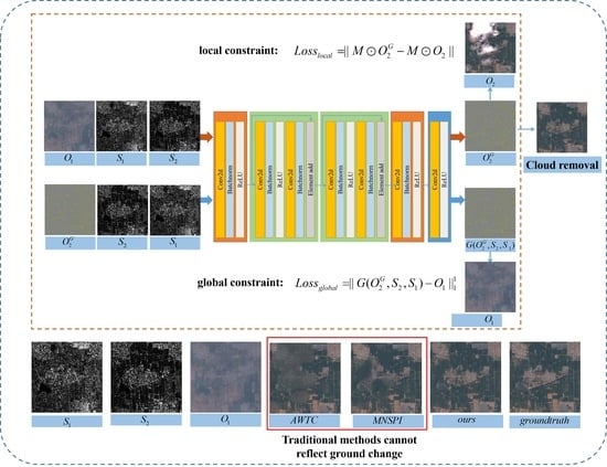
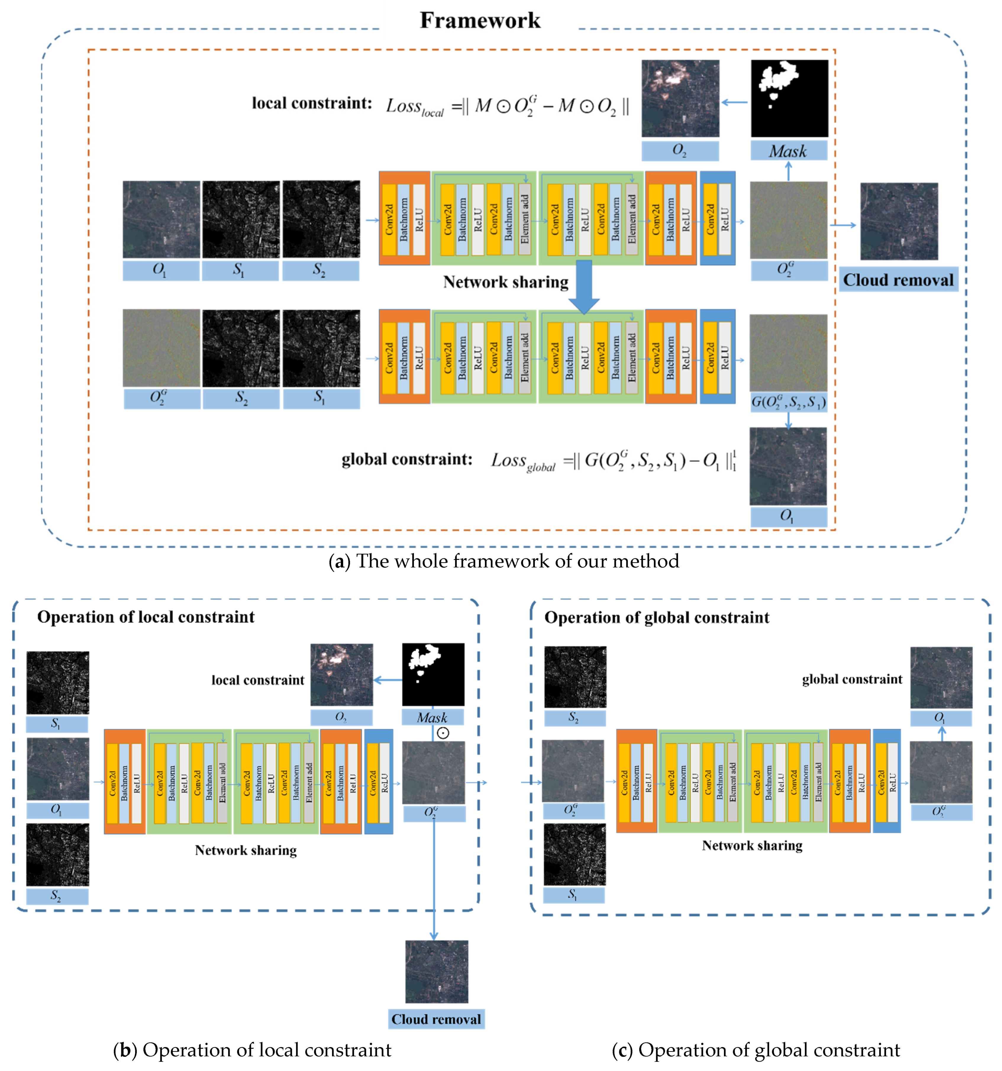
Instead of the ideal training condition where in training datasets have no missing information, we attempt to deal with a more general situation, where the given has missing information and the training dataset is unavailable. We aim to obtain which is the reconstruction result of . Here we also make use of , and as reference images and introduce a deep neural network, which is denoted as . The whole framework of our method is displayed in Figure 1a.
First, we implement a cloud detection algorithm to get the missing information mask from :
Then, we concatenate the images in the sequence of , , and treat them as the input of network for a simulated output : which is described in Equation (4):
With the cloud mask and the simulated output map , we make use of the residual information of to construct a local optimization term to optimize the simulated output in the network . The reconstruction term is described in Equation (5):
means the Hadamard product operation. With Equation (5), we expect that network can learn the ground information change between and , and further impose the real-time ground information to the expected cloud removal results . The process of Equations (4)−(5) is displayed in Figure 1b.
However, the remaining information in is local so it cannot perfectly constrain the global information and continuity of cloud removal results. To further guarantee the authority and reflect the ground information changes in , we concatenate the images in the sequence of , and , and feed them again to the same network for another output :
Then, another optimization term is constructed with this output and to constrain the global information and continuity, which is described in Equation (7):
Assume that can reflect the local ground information change with the sole Equation (5). By transforming back to with Equations (6) and (7), we expect that this global optimization term can further constrain the network to diffuse the knowledge of ground information change from the local areas to cloudy areas, so that the results can reflect the global ground information changes between and . The process of Equation (6) is displayed in Figure 1c.
For further continuity of the cloud removal result , we then impose a total variation term to the optimization term. The total optimization term can be described as follows:
Finally, different from those deep learning methods who retain the network G after optimization for further application such as Equations (1) and (2), we abandon the network but only retain the final optimization output as the final reconstruction result. The action is described in Equation (9):
The whole process needs no training datasets, but only the target image with clouds and reference images. Compared with those deep learning methods, our method does not need to consider transfer learning when it comes to novel images outside the domain of training datasets, ensuring the flexibility of the proposed method.
2.3. Network Structure
In the proposed method, we use a simple network with five main consecutive blocks. In the first and fourth block, there are a convolution operation layer, a batch normalization layer and a non-linear activation layer. The second and the third blocks are the residual blocks whose structure is displayed in Figure 1. After processed by two convolution and batch normalization blocks, the input feature map adds the output feature map as the final output. The aim of the residual blocks is to avoid the gradient vanishing problem. The final block has a convolution operation layer and a non-linear activation layer to obtain the target reconstruction result. The total network design is presented in Figure 1.
3. Experiments
3.1. Experiment Settings
3.1.1. Data Introduction
From the Sentinel 1 and Sentinel 2 satellites, we collected eight groups of SAR images and optical images from two periods, respectively, for the simulation experiments and two groups of SAR and optical images from two periods for real data experiments. The gap between the two periods is less than one year. Within one period, the gap of the acquired time of SAR and optical images is constrained within a week to confirm that SAR and optical images from the same time share the same ground information. SAR images are obtained in the mode of IW and have two bands which are, respectively, VV and VH. We preprocessed the SAR images with deburst, calibration, terrain correction and finally unified the spatial resolution into 10 m. The optical images have the resolution of 10 m and we only chose the R, G and B bands in the experiments for the sake of simplification. We cropped patches with the size of 2000 × 2000 in the same areas of optical and SAR images from the two periods. The acquisition time of these images is listed in Table 1.
3.1.2. Mask Production
For the simulation reconstruction experiments, we collected the optical images with cloud corruption from Sentinel 2 and made use of Fmask 4.3 algorithm to catch the masks of clouds and their shadows in these images. Then, we cropped the patches randomly with the size of 2000 × 2000 from these cloud masks. We filtered 8 patches which have around 30% of cloud areas and their corresponding optical patches. Furthermore, in the eight groups of optical and SAR images, we selected one optical image in each group and replaced the information of some areas with the corresponding areas of the optical cloud patch to simulate the corrupted optical images. For the real data experiment, we directly made use of Fmask 4.3 algorithm to detect the clouds and their shadow in the image to make the cloud mask.
3.1.3. Evaluation Methods
We made use of four popular evaluation indexes to assess the reconstruction results of the proposed method. They are, respectively, peak-signal-to-noise ratio (PSNR), Structure, Similarity index (SSIM), Spectral Angle Mapper (SAM) and Correlation Coefficient (CC). They can evaluate the spectral and spatial fidelity of the cloud removal results. For PSNR, SSIM and CC, a higher score indicates a better result. For SAM, a lower score means the better result.
3.1.4. Implementation Details
We conducted our experiments under the framework of Pytorch 1.0 with one GPU of RTX 2080Ti. The reconstruction result was obtained by optimizing the output of network with Adam optimizer. The learning rate of the network in our method was set as 0.001 and the number of optimization epochs was set as 2000.
3.1.5. Comparison Methods
3.2. Simulation Experiment Results
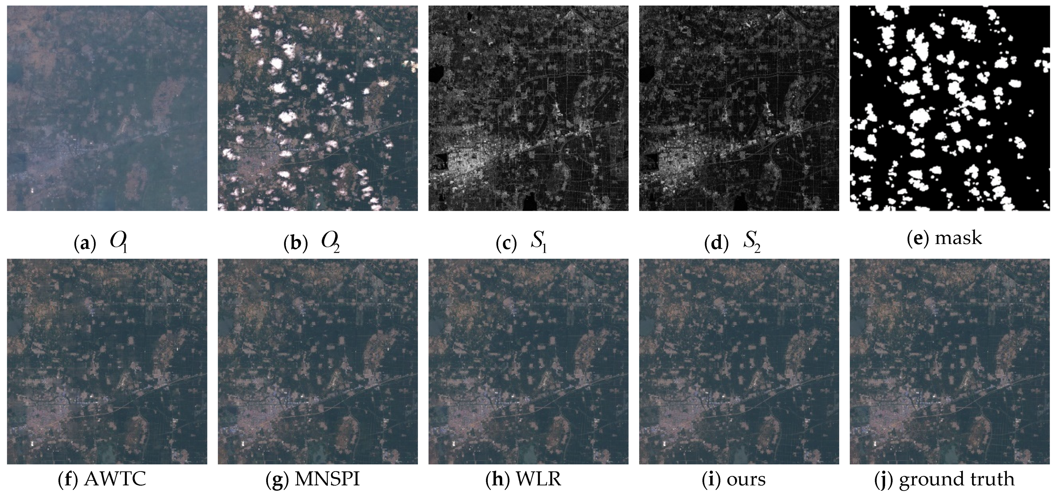
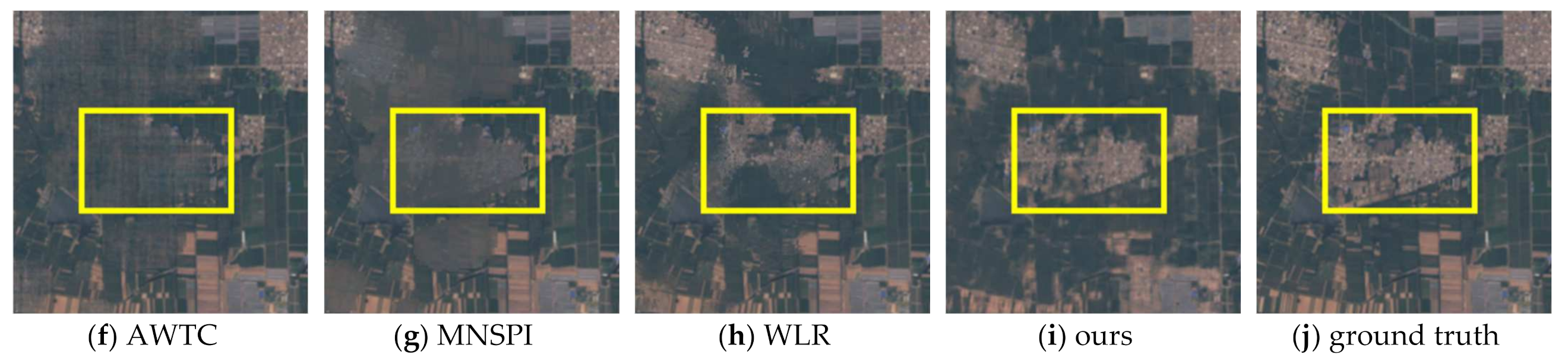
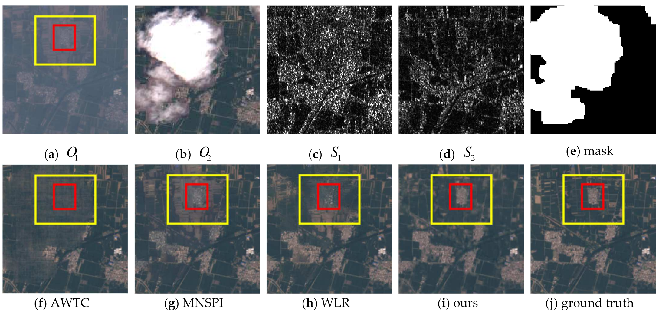
The experiment results are displayed in Figure 2. Figure 2a,b presents the simulated optical image with missing information and the multitemporal optical image from adjacent period. Figure 2c−d shows the SAR images obtained from the same time as optical images shown in Figure 2a−b. Figure 2e is the cloud mask. Figure 2 f−h, respectively, displays the reconstruction results of AWTC, MNSPI and WLR. Figure 2i is the result of the proposed method and Figure 2j displays the ground truth of corrupted optical image. We selected two areas and magnify them in Figure 3 and Figure 4.
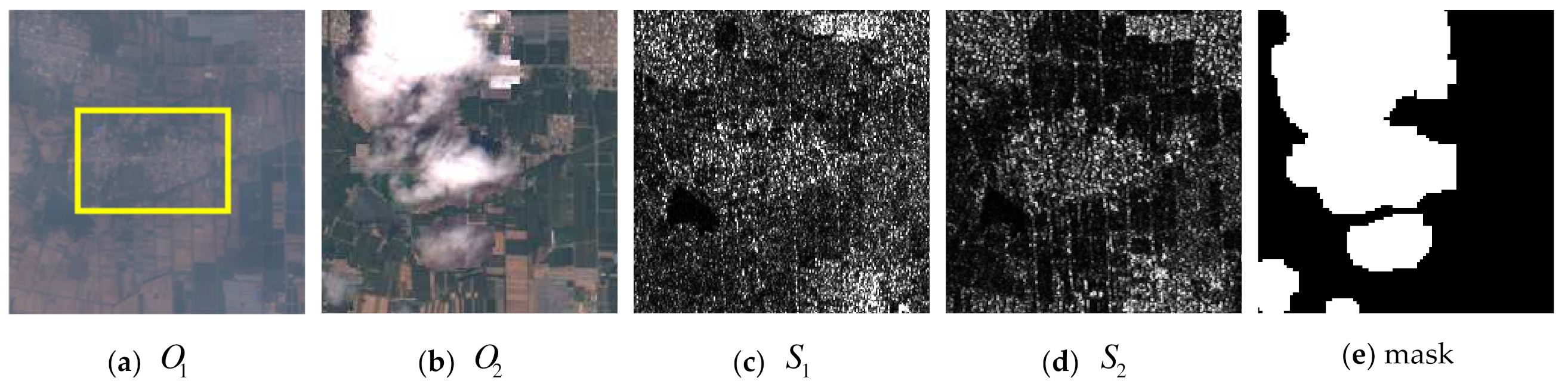
In Figure 3, the area boxed in yellow is mainly the town area. In the ground truth image, the spectral information of the town area and surrounding agricultural area is vividly different from each other. However, in the reference image , the town area and the surrounding agricultural area share the similar spectral information and it is very easy to mix them up. Therefore, in the results of WLR and MNSPI, the boxed town area is reconstructed as agricultural land because they can only take as reference image. Even worse, AWTC only obtains blurry results in the gap areas. The proposed method, on the other hand, can distinguish the town area from the surrounding agricultural area and the cloud removal result has accurate spectral information thanks to the reference images and . The above example indicates that reconstruction process of traditional methods is just information cloning from the optical images from adjacent periods and does not take the ground information change into consideration. Therefore, the traditional multitemporal-based methods may not be practical in real applications. Our method can reflect the ground information changes which are displayed in two SAR images from two periods.
Another example is the area displayed in Figure 4. The area boxed in red is the town area while the surrounding area boxed in yellow is the agricultural area. In the ground truth image, the town area and the agricultural area has obviously different spectral information while in the reference image , the two areas share the same spectral information. WLR reconstructs the town area into the agricultural area while the agricultural area in the result of MNSPI has wrong spectral information. The result of AWTC is blurry because AWTC cannot deal well with images with large size. The proposed method perfectly distinguishes the town area and agricultural area, and the result has true spectral information.
Table 2 lists the quantitative evaluation of our method and three traditional multitemporal-based methods. We mark the highest score in each index in bold and the second highest score with underline. Our method obtains highest scores in all four evaluation indexes. Simulation experiments indicate that the introduction of auxiliary multitemporal SAR images is of vital importance to reflect the ground change in the results.
3.3. Real Experiment Results
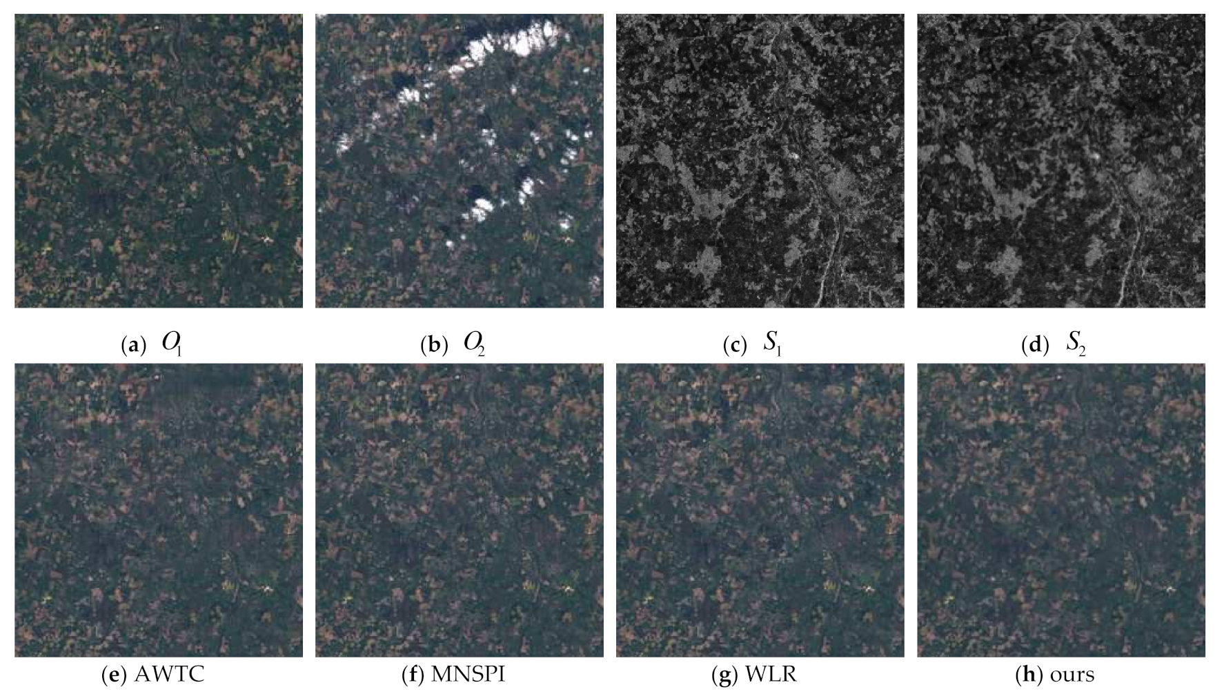
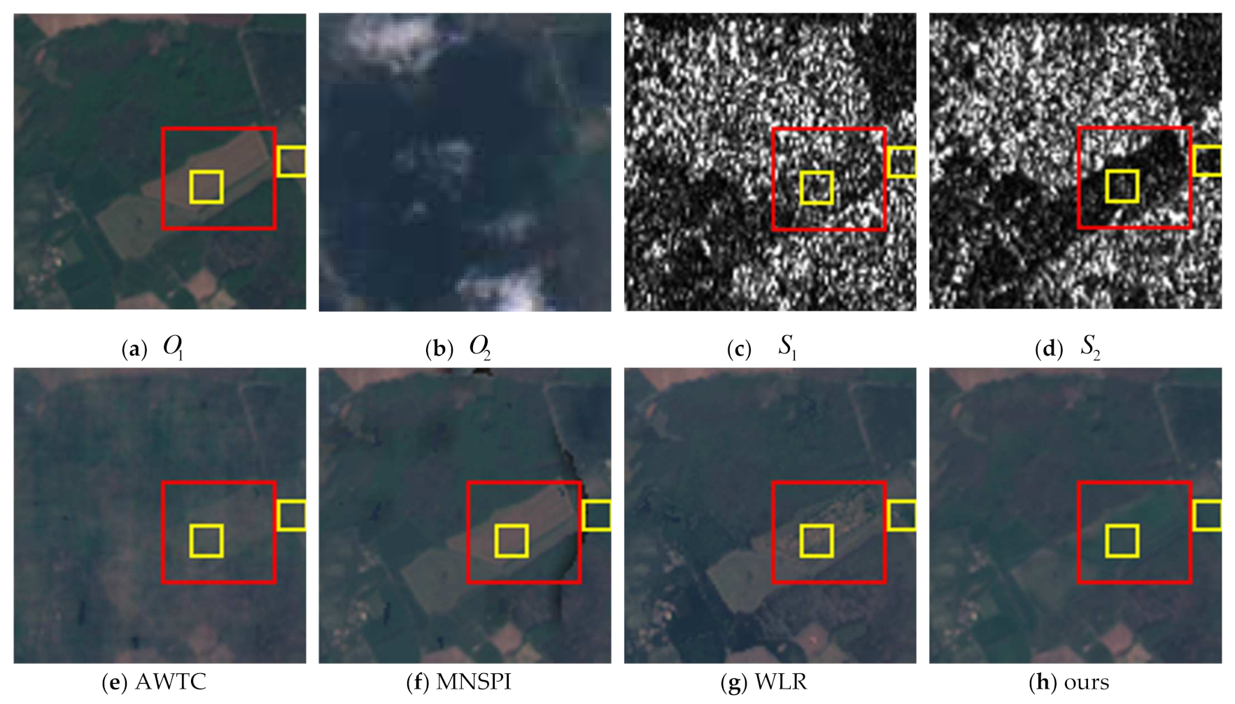
Results of real data experiments are displayed in Figure 5. Figure 5a−d, shows, respectively, the corrupted optical image, the reference optical image and SAR images from two periods. Figure 5e−g displays the results of AWTC, MNSPI and WLR. The result of our method is presented in Figure 5h. We magnify a selected area of Figure 5 in Figure 6 for further observation.
We can observe from two SAR images that the ground information in the area boxed in red has changed between the two periods. Due to the fact that no ground truth image can be referred in this set of experiments, we cannot directly compare the correctness of each method. However, we find in and that the two areas in the yellow box share the same ground information in both and. In the results of MNSPI and WLR, the ground objects in two yellow boxes are different. AWTC again cannot deal with large images and obtains blurry results. The proposed method, on the other hand, has ground objects with the same spectral information in the two yellow boxes, confirming the accuracy of our cloud removal result.
4. Discussion
To further explore the function of each data and module of our method, we conduct the ablation experiment of the proposed method. Then we discuss the efficiency of our method.
4.1. Ablation Study about Loss Function
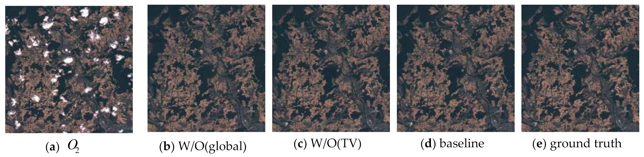
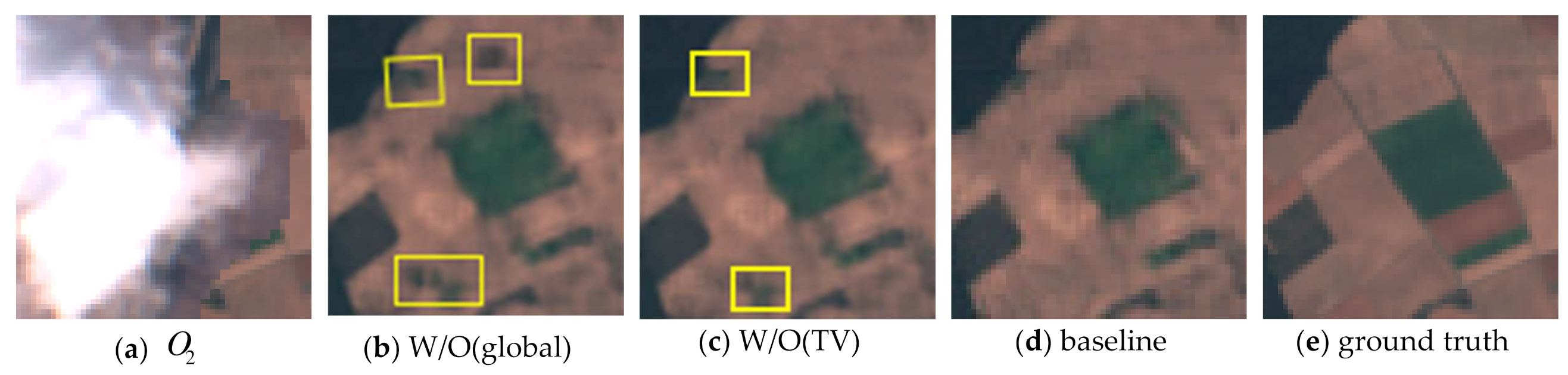
In this section, we analyze the contributions of each loss function in the proposed method with the eight groups of multitemporal SAR-optical images used in the simulation experiment. The model, which contains all three loss functions, is set as the baseline model. Then we denote the model without total variation term as W/O(TV). The model without global loss function as W/O(global). On the other hand, we have to admit that local loss function contributes mainly to the cloud removal results and without the local loss function, no results will be obtained. Therefore, we cannot do the ablation study on the local loss function term. Table 3 lists the quantitative evaluation results of above ablation models. We mark the highest scores in bold. The evaluation results indicate that all loss functions contribute positively to the proposed method. Figure 6 displays the cloud removal results of the proposed method and three ablation models. Figure 7a displays the cloudy image. Figure 7b−c shows, respectively, the results of models W/O(global) and W/O(TV). Figure 7d−e is the result of full model and the ground truth. We select an area from Figure 6 and display it in Figure 8. It can be viewed from Figure 8 that global loss function contributes a lot to relieving the overfitting of model. Without global loss function, the model may generate some nonexistent ground information which are boxed in yellow. Although TV loss function may not contribute as much as global loss function, it also helps to relieve the overfitting of model. We can see from Figure 8c that without TV loss function, there still remains some artifacts in the cloud removal result.
4.2. Ablation Study about Reference Data
In this part, we further analyze the function of reference images used in the framework with the eight groups of multitemporal SAR and optical images. For the sake of fairness, we set the model with only local loss function as baseline because the construction of global loss function needs all reference images. With global loss function, we cannot compare the contribution of each reference image.
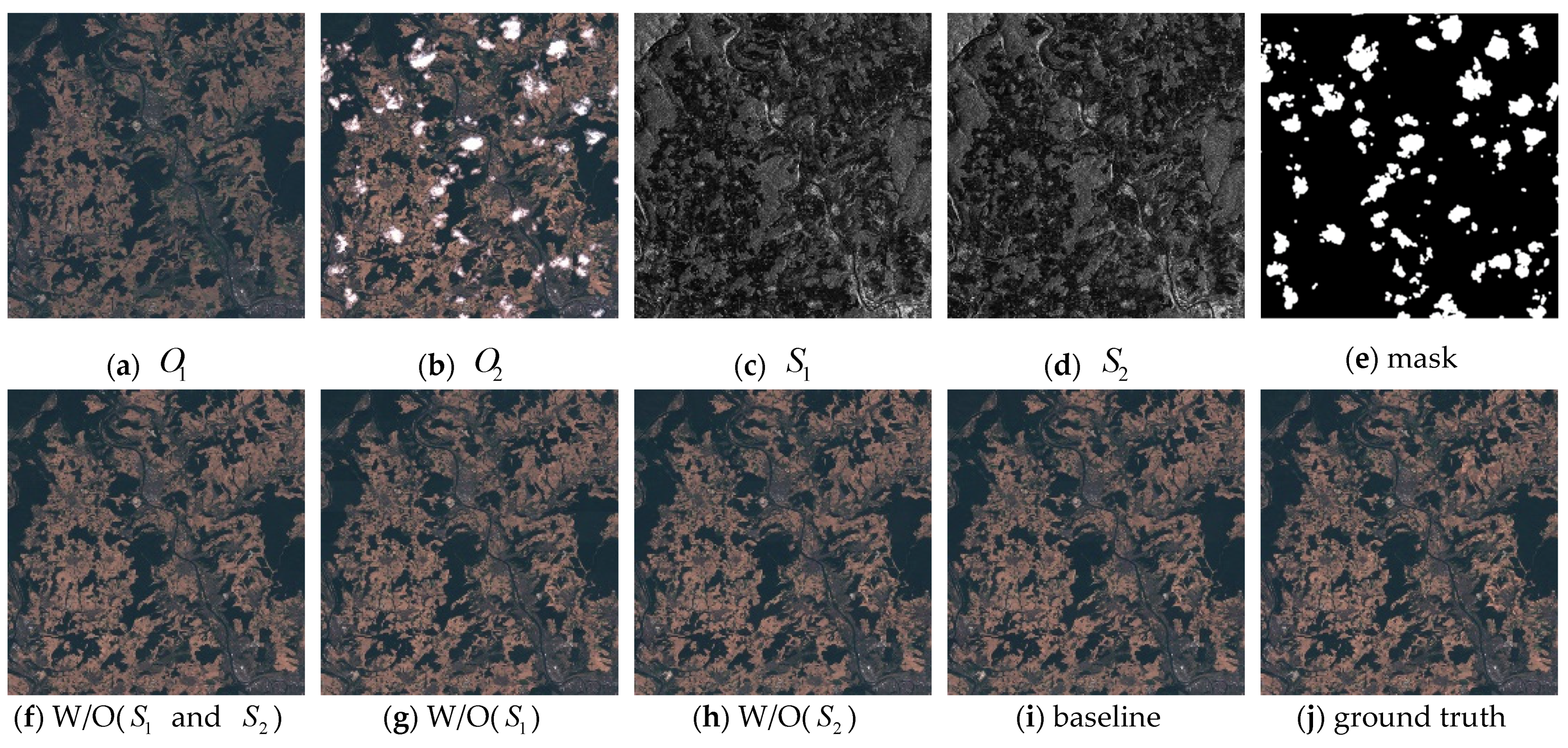
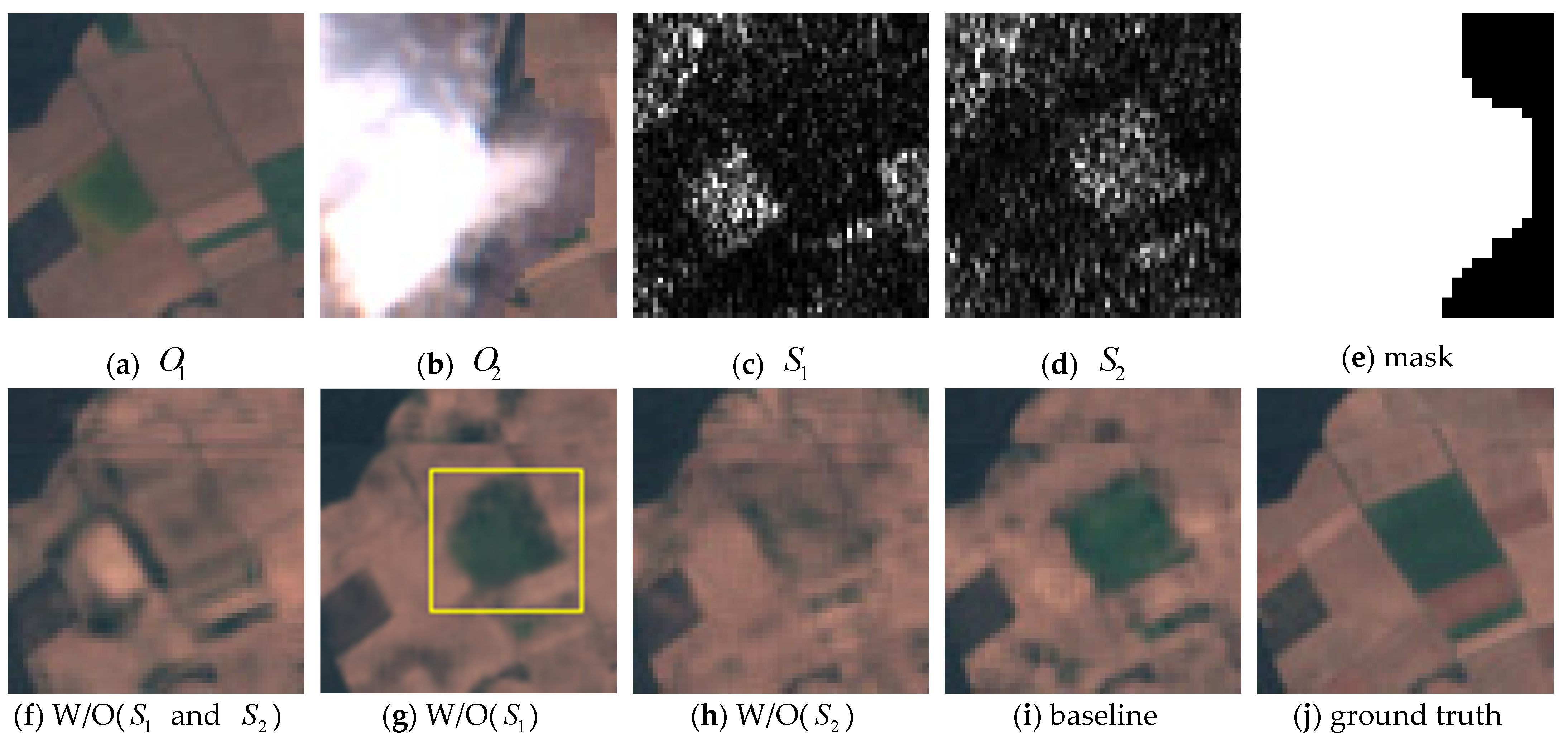
The model without and is denoted as W/O(and). We denote the model without as W/O( ) and the model without as W/O( ). Figure 9 displays the results of the baseline model and three ablation models. Figure 9a–d shows, respectively, the multitemporal SAR and optical images. Figure 9e is the cloud mask. Figure 9f–i displays the results of four ablation models and the baseline model. Figure 9j is the ground truth image. We select an area from the above images and display it in Figure 10. It can be observed from two SAR images that obvious ground information change occurs between two periods, which is boxed in red. Results of models W/O( ) and W/O(and) cannot reflect this ground information change because reference images do not contain the ground information of. The result of model W/O( ) reflects the ground information change in the reconstruction result and its result is satisfying in terms of visual evaluation. However, the shape of some ground objects, which is boxed in yellow, is not the same as ground truth. The reason may be that W/O( ) retains the corresponding spatial information of in the reconstructed areas of. However, as is known to all, the shapes of objects in SAR images and optical images are different due to their different imaging process. W/O( ) does not take the spatial information difference into consideration so that spatial information of some reconstruction areas is warped. The baseline model, with the aid of all reference images, can obtain results whose ground information has an accurate shape, outperforming all ablation models. We also evaluate our method and three ablation models quantitatively and list the quantitative evaluation results in Table 4. The highest scores are marked in bold and the second highest scores are marked with underline. The baseline model undoubtedly achieves the highest scores in all four indexes and outperforms the remaining three ablation models by a large extent. The ablation models indicate that all reference images including, and are of vital importance in the proposed method.
4.3. Time Cost
Despite the fact that the proposed method can take ground information change into consideration and also obtain results with both good quantitative and qualitative evaluation, we have to admit that the above achievements are at the cost of efficiency. Different from those deep learning methods that process images in a feed-forward manner with a well-trained network, the proposed method adopts an image-optimization process which processes the original images in a backward-propagation manner because there is no extra dataset to train the network. To process an image with a size of 2000 × 2000, deep learning methods may only need several seconds while the proposed method will need several minutes. Table 5 lists the time cost of the proposed method and two comparison methods on one image with a size of 2000 × 2000. WLR only takes several seconds while MNSPI takes tens of seconds. The proposed method takes hundreds of seconds, an excessive amount of time. We will seek a solution for the efficiency of our method in future work.
5. Conclusions
In this paper, we proposed a method for cloud removal of optical images from Sentinel-2 satellites. The proposed method takes advantages of multitemporal optical images from Sentinel-2 satellites and multitemporal SAR images from Sentinel-1 satellites as reference for the reconstruction. The whole process is conducted in a deep neural network and does not need a training dataset. As far as we know, our method is the first multitemporal-based method that can reflect the ground information change in practical cloud removal tasks without large training datasets. The success of simulation and real data experiments confirms the superiority of applicability of the proposed method.
In our future work, we would collect a large training dataset to train a deep neural network that can operate in a forward manner and reflect the ground information change in the reconstruction results. Moreover, we will modify the network structure for more accurate results.
Author Contributions
Conceptualization, J.G., Y.Y., T.W., G.Z.; formal analysis, Y.Y., G.Z.; funding acquisition J.G.; investigation, J.G., Y.Y.; methodology, J.G., Y.Y., T.W.; project administration, J.G.; resources, J.G.; supervision, Y.Y., T.W.; validation, J.G.; writing—original draft, J.G., Y.Y.; writing—review and editing, J.G., Y.Y., T.W., G.Z.; All authors have read and agreed to the published version of the manuscript.
Funding
This research was funded by National Natural Science Foundation of China, grant number 62071341.
Conflicts of Interest
The authors declare no conflict of interest.
References
- Du, L.; Tian, Q.; Yu, T.; Meng, Q.; Jancso, T.; Udvardy, P.; Huang, Y. A comprehensive drought monitoring method integrating modis and trmm data. Int. J. Appl. Earth Obs. Geoinf. 2013, 23, 245–253. [Google Scholar] [CrossRef]
- Rapinel, S.; Hubert-Moy, L.; Clément, B. Combined use of lidar data and multispectral earth observation imagery for wetland habitat mapping. Int. J. Appl. Earth Obs. Geoinf. 2015, 37, 56–64. [Google Scholar] [CrossRef]
- Rodríguez-Veiga, P.; Quegan, S.; Carreiras, J.; Persson, H.J.; Fransson, J.E.; Hoscilo, A.; Ziółkowski, D.; Stereńczak, K.; Lohberger, S.; Stängel, M. Forest biomass retrieval approaches from earth observation in different biomes. Int. J. Appl. Earth Obs. Geoinf. 2019, 77, 53–68. [Google Scholar] [CrossRef]
- Kogan, F.; Kussul, N.; Adamenko, T.; Skakun, S.; Kravchenko, O.; Kryvobok, O.; Shelestov, A.; Kolotii, A.; Kussul, O.; Lavrenyuk, A. Winter wheat yield forecasting in ukraine based on earth observation, meteorological data and biophysical models. Int. J. Appl. Earth Obs. Geoinf. 2013, 23, 192–203. [Google Scholar] [CrossRef]
- Pradhan, S. Crop area estimation using gis, remote sensing and area frame sampling. Int. J. Appl. Earth Obs. Geoinf. 2001, 3, 86–92. [Google Scholar] [CrossRef]
- Ju, J.; Roy, D.P. The availability of cloud-free landsat etm+ data over the conterminous united states and globally. Remote Sens. Environ. 2008, 112, 1196–1211. [Google Scholar] [CrossRef]
- Shen, H.; Li, X.; Cheng, Q.; Zeng, C.; Yang, G.; Li, H.; Zhang, L. Missing information reconstruction of remote sensing data: A technical review. IEEE Geosci. Remote Sens. Mag. 2015, 3, 61–85. [Google Scholar] [CrossRef]
- Wang, L.; Qu, J.J.; Xiong, X.; Hao, X.; Xie, Y.; Che, N. A new method for retrieving band 6 of aqua modis. IEEE Geosci. Remote Sens. Lett. 2006, 3, 267–270. [Google Scholar] [CrossRef]
- Shen, H.; Zeng, C.; Zhang, L. Recovering reflectance of aqua modis band 6 based on within-class local fitting. IEEE J. Sel. Top. Appl. Earth Obs. Remote Sens. 2010, 4, 185–192. [Google Scholar] [CrossRef]
- Zhang, C.; Li, W.; Travis, D. Gaps-fill of slc-off landsat etm+ satellite image using a geostatistical approach. Int. J. Remote Sens. 2007, 28, 5103–5122. [Google Scholar] [CrossRef]
- Yu, C.; Chen, L.; Su, L.; Fan, M.; Li, S. Kriging interpolation method and its application in retrieval of modis aerosol optical depth. In Proceedings of the 19th International Conference on Geoinformatics, Shanghai, China, 24–26 June 2011; IEEE: Piscataway, NJ, USA, 2011; pp. 1–6. [Google Scholar]
- Bertalmio, M.; Sapiro, G.; Caselles, V.; Ballester, C. Image inpainting. In Proceedings of the 27th Annual Conference on Computer Graphics and Interactive Techniques, New Orleans, LA, USA, 23–28 July 2000; pp. 417–424. [Google Scholar]
- Ballester, C.; Bertalmio, M.; Caselles, V.; Sapiro, G.; Verdera, J. Filling-in by joint interpolation of vector fields and gray levels. IEEE Trans. Image Process. 2001, 10, 1200–1211. [Google Scholar] [CrossRef] [Green Version]
- Chan, T.F.; Shen, J. Nontexture inpainting by curvature-driven diffusions. J. Vis. Commun. Image Represent. 2001, 12, 436–449. [Google Scholar] [CrossRef]
- Shen, J.; Chan, T.F. Mathematical models for local nontexture inpaintings. SIAM J. Appl. Math. 2002, 62, 1019–1043. [Google Scholar] [CrossRef]
- Bugeau, A.; Bertalmío, M.; Caselles, V.; Sapiro, G. A comprehensive framework for image inpainting. IEEE Trans. Image Process. 2010, 19, 2634–2645. [Google Scholar] [CrossRef]
- Efros, A.A.; Leung, T.K. Texture synthesis by non-parametric sampling. In Proceedings of the Seventh IEEE International Conference on Computer Vision, Kerkyra, Greece, 20–27 September 1999; IEEE: Piscataway, NJ, USA, 1999; pp. 1033–1038. [Google Scholar]
- Criminisi, A.; Pérez, P.; Toyama, K. Region filling and object removal by exemplar-based image inpainting. IEEE Trans. Image Process. 2004, 13, 1200–1212. [Google Scholar] [CrossRef]
- Zhang, J.; Clayton, M.K.; Townsend, P.A. Functional concurrent linear regression model for spatial images. J. Agric. Biol. Environ. Stat. 2011, 16, 105–130. [Google Scholar] [CrossRef]
- Zhang, J.; Clayton, M.K.; Townsend, P.A. Missing data and regression models for spatial images. IEEE Trans. Geosci. Remote Sens. 2014, 53, 1574–1582. [Google Scholar] [CrossRef]
- Lorenzi, L.; Melgani, F.; Mercier, G. Missing-area reconstruction in multispectral images under a compressive sensing perspective. IEEE Trans. Geosci. Remote Sens. 2013, 51, 3998–4008. [Google Scholar] [CrossRef]
- Li, X.; Shen, H.; Zhang, L.; Zhang, H.; Yuan, Q.; Yang, G. Recovering quantitative remote sensing products contaminated by thick clouds and shadows using multitemporal dictionary learning. IEEE Trans. Geosci. Remote Sens. 2014, 52, 7086–7098. [Google Scholar]
- Chen, J.; Jönsson, P.; Tamura, M.; Gu, Z.; Matsushita, B.; Eklundh, L. A simple method for reconstructing a high-quality ndvi time-series data set based on the savitzky–golay filter. Remote Sens. Environ. 2004, 91, 332–344. [Google Scholar] [CrossRef]
- Jönsson, P.; Eklundh, L. Timesat—A program for analyzing time-series of satellite sensor data. Comput. Geosci. 2004, 30, 833–845. [Google Scholar] [CrossRef] [Green Version]
- Uzkent, B.U.; Sarukkai, V.S.; Jain, A.J.; Ermon, S.E. Cloud removal in satellite images using spatiotemporal generative networks. In Proceedings of the 2020 IEEE Winter Conference on Applications of Computer Vision (WACV), Snowmass, CO, USA, 1–5 March 2020; IEEE: Piscataway, NJ, USA, 2020. [Google Scholar]
- Singh, P.; Komodakis, N. Cloud-gan: Cloud removal for sentinel-2 imagery using a cyclic consistent generative adversarial networks. In Proceedings of the IGARSS 2018–2018 IEEE International Geoscience and Remote Sensing Symposium, Valencia, Spain, 22–27 July 2018; IEEE: Piscataway, NJ, USA, 2018; pp. 1772–1775. [Google Scholar]
- Liu, L.; Lei, B. Can sar images and optical images transfer with each other? In .Proceedings of the IGARSS 2018-2018 IEEE International Geoscience and Remote Sensing Symposium, Valencia, Spain, 22–27 July 2018; IEEE: Piscataway, NJ, USA, 2018; pp. 7019–7022. [Google Scholar]
- Li, W.; Li, Y.; Chan, J.C.-W. Thick cloud removal with optical and sar imagery via convolutional-mapping-deconvolutional network. IEEE Trans. Geosci. Remote Sens. 2019, 58, 2865–2879. [Google Scholar] [CrossRef]
- Gao, J.; Yuan, Q.; Li, J.; Zhang, H.; Su, X. Cloud removal with fusion of high resolution optical and sar images using generative adversarial networks. Remote Sens. 2020, 12, 191. [Google Scholar] [CrossRef] [Green Version]
- Turnes, J.N.; Castro, J.D.B.; Torres, D.L.; Vega, P.J.S.; Feitosa, R.Q.; Happ, P.N. Atrous cgan for sar to optical image translation. IEEE Geosci. Remote Sens. Lett. 2020. [Google Scholar] [CrossRef]
- Bermudez, J.; Happ, P.; Oliveira, D.; Feitosa, R. Sar to optical image synthesis for cloud removal with generative adversarial networks. ISPRS Ann. Photogramm. Remote Sens. Spat. Inf. Sci. 2018, 4. [Google Scholar] [CrossRef] [Green Version]
- Isola, P.; Zhu, J.-Y.; Zhou, T.; Efros, A.A. Image-to-image translation with conditional adversarial networks. In Proceedings of the IEEE Conference on Computer Vision and Pattern Recognition, Honolulu, HI, USA, 21–26 July 2017; IEEE: Piscataway, NJ, USA, 2017; pp. 1125–1134. [Google Scholar]
- Zhu, J.-Y.; Park, T.; Isola, P.; Efros, A.A. Unpaired image-to-image translation using cycle-consistent adversarial networks. In Proceedings of the IEEE International Conference on Computer Vision, Venice, Italy, 22–29 October 2017; IEEE: Piscataway, NJ, USA, 2017; pp. 2223–2232. [Google Scholar]
- He, W.; Yokoya, N. Multi-temporal sentinel-1 and-2 data fusion for optical image simulation. ISPRS Int. J. Geo-Inf. 2018, 7, 389. [Google Scholar] [CrossRef] [Green Version]
- Bermudez, J.D.; Happ, P.N.; Feitosa, R.Q.; Oliveira, D.A. Synthesis of multispectral optical images from sar/optical multitemporal data using conditional generative adversarial networks. IEEE Geosci. Remote Sens. Lett. 2019, 16, 1220–1224. [Google Scholar] [CrossRef]
- Xia, Y.; Zhang, H.; Zhang, L.; Fan, Z. Cloud removal of optical remote sensing imagery with multitemporal sar-optical data using x-mtgan. In Proceedings of the IGARSS 2019–2019 IEEE International Geoscience and Remote Sensing Symposium, Yokohama, Japan, 28 July–2 August 2019; IEEE: Piscataway, NJ, USA, 2019; pp. 3396–3399. [Google Scholar]
- Meraner, A.; Ebel, P.; Zhu, X.X.; Schmitt, M. Cloud removal in sentinel-2 imagery using a deep residual neural network and sar-optical data fusion. ISPRS J. Photogramm. Remote Sens. 2020, 166, 333–346. [Google Scholar] [CrossRef]
- Ng, M.K.-P.; Yuan, Q.; Yan, L.; Sun, J. An adaptive weighted tensor completion method for the recovery of remote sensing images with missing data. IEEE Trans. Geosci. Remote Sens. 2017, 55, 3367–3381. [Google Scholar] [CrossRef]
- Zhu, X.; Gao, F.; Liu, D.; Chen, J. A modified neighborhood similar pixel interpolator approach for removing thick clouds in landsat images. IEEE Geosci. Remote Sens. Lett. 2011, 9, 521–525. [Google Scholar] [CrossRef]
- Zeng, C.; Shen, H.; Zhang, L. Recovering missing pixels for landsat etm+ slc-off imagery using multi-temporal regression analysis and a regularization method. Remote Sens. Environ. 2013, 131, 182–194. [Google Scholar] [CrossRef]
Figure 1.
The flowchart of our method.

Figure 2.
The global view of simulation experiment results.

Figure 3.
Magnified area 1 of simulation experiment results. Area boxed in yellow is the town area. In , the town area and the surrounding area share the same spectral information while in the ground truth they are different. Only the proposed method can differentiate the town area and the surrounding area.


Figure 4.
Magnified area 2 of simulation experiment results. The area boxed in red is the town area while the surrounding area boxed in yellow is the agricultural area. In they share the same spectral information while in the ground truth they have totally different spectral information. The three comparison methods either reconstruct the town area into agricultural area or the agriculture area into town area. Our method can distinguish the two kinds of ground objects.

Figure 5.
Real experiment results of cloud removal.

Figure 6.
Magnified area of real experiment results. From and , we can see obvious ground information change. Moreover, we observe from , and ,that the two areas boxed in yellow share the same ground information. In the results of three comparison methods, the two areas in yellow boxes are different while in the result of our method, the two areas share the same spectral information.

Figure 7.
Results of ablation models about loss functions.

Figure 8.
Magnified area from Figure 7. Results of model W/O(global) and W/O(TV) have vivid artifacts while the proposed method has no artifacts in the result.
Figure 8.
Magnified area from Figure 7. Results of model W/O(global) and W/O(TV) have vivid artifacts while the proposed method has no artifacts in the result.

Figure 9.
Simulation experiment results of ablation models.

Figure 10.
Magnified area from Figure 9. Every reference image contributes positively to the final result.
Figure 10.
Magnified area from Figure 9. Every reference image contributes positively to the final result.


Table 1.
Acquisition time of images.
| Simulation exp | ||||
|---|---|---|---|---|
| 1 | 22 March 2020 | 8 July 2020 | 23 March 2020 | 6 July 2020 |
| 2 | 16 November 2019 | 2 May 2020 | 14 November 2019 | 2 May 2020 |
| 3 | 20 October 2019 | 23 May 2020 | 19 October 2019 | 21 May 2020 |
| 4 | 1 November 2019 | 13 December 2019 | 31 October 2019 | 10 December 2019 |
| 5 | 18 October 2019 | 5 December 2019 | 19 October 2019 | 8 December 2019 |
| 6 | 24 March 2020 | 5 April 2020 | 26 March 2020 | 5 April 2020 |
| 7 | 27 August 2019 | 9 August 2020 | 23 August 2019 | 7 August 2020 |
| 8 | 31 August 2019 | 2 July 2020 | 5 September 2019 | 1 July 2020 |
| Real data exp | ||||
| 1 | 09 April 2021 | 03 May 2021 | 08 April 2021 | 03 May 2021 |
| 2 | 20 April 2021 | 14 April 2021 | 23 April 2021 | 15 April 2021 |
Table 2.
Quantitative evaluation of simulation results.
| PSNR | SSIM | CC | SAM | |
|---|---|---|---|---|
| WLR | 35.9515 * | 0.9679 * | * 0.9782 | * 0.2894 |
| MNSPI | 34.9646 | 0.9661 | 0.9721 | 0.3617 |
| AWTC | 32.6143 | 0.9487 | 0.9596 | 0.4800 |
| Ours | 37.3142 * | 0.9748 * | 0.9842 * | 0.2586 * |
* The best scores are marked in bold while the second highest are marked with underline. Our method achieves all best scores in all four indexes.
Table 3.
Quantitative evaluation of ablation models about loss function.
| PSNR | SSIM | CC | SAM | |
|---|---|---|---|---|
| W/O(TV) | 37.2542 | 0.9747 | 0.9841 | 0.2591 |
| W/O(global) | 37.2075 | 0.9746 | 0.9841 | 0.2592 |
| Baseline | 37.3142 | 0.9748 | 0.9842 | 0.2586 |
The best scores are marked in bold while the second highest are marked with underline. The full model achieves all best scores in all four indexes.
Table 4.
Quantitative evaluation of ablation models about reference images.
| PSNR | SSIM | CC | SAM | |
|---|---|---|---|---|
| W/O( and ) | 36.3542 | 0.9724 | 0.9805 | 0.2803 |
| W/O() | 37.1386 | 0.9743 | 0.9839 | 0.2598 |
| W/O() | 36.4235 | 0.9725 | 0.9808 | 0.2745 |
| Ours | 37.1953 | 0.9746 | 0.9841 | 0.2593 |
The best scores are marked in bold while the second highest are marked with underline. The full model achieves all best scores in all four indexes.
Table 5.
Time cost of three comparison methods and our method.
| WLR | MNSPI | AWTC | Ours | |
|---|---|---|---|---|
| Time | <4 s | 26 s | 183 s | 842 s |
Publisher’s Note: MDPI stays neutral with regard to jurisdictional claims in published maps and institutional affiliations. |
© 2021 by the authors. Licensee MDPI, Basel, Switzerland. This article is an open access article distributed under the terms and conditions of the Creative Commons Attribution (CC BY) license (https://creativecommons.org/licenses/by/4.0/).
Share and Cite
MDPI and ACS Style
Gao, J.; Yi, Y.; Wei, T.; Zhang, G. Sentinel-2 Cloud Removal Considering Ground Changes by Fusing Multitemporal SAR and Optical Images. Remote Sens. 2021, 13, 3998. https://0-doi-org.brum.beds.ac.uk/10.3390/rs13193998
AMA Style
Gao J, Yi Y, Wei T, Zhang G. Sentinel-2 Cloud Removal Considering Ground Changes by Fusing Multitemporal SAR and Optical Images. Remote Sensing. 2021; 13(19):3998. https://0-doi-org.brum.beds.ac.uk/10.3390/rs13193998
Chicago/Turabian StyleGao, Jianhao, Yang Yi, Tang Wei, and Guanhao Zhang. 2021. "Sentinel-2 Cloud Removal Considering Ground Changes by Fusing Multitemporal SAR and Optical Images" Remote Sensing 13, no. 19: 3998. https://0-doi-org.brum.beds.ac.uk/10.3390/rs13193998
Note that from the first issue of 2016, this journal uses article numbers instead of page numbers. See further details here.