SMOS Brightness Temperature Monitoring Quality Control Review and Enhancements

Abstract

Brightness temperature (Tb) observations from the European Space Agency (ESA) Soil Moisture Ocean Salinity (SMOS) instrument are passively monitored in the European Centre for Medium-range Weather Forecasts (ECMWF) Integrated Forecasting System (IFS). Several quality control procedures are performed to screen out poor quality data and/or data that cannot accurately be simulated from the numerical weather prediction (NWP) model output. In this paper, these quality control procedures are reviewed, and enhancements are proposed, tested, and evaluated. The enhancements presented include improved sea ice screening, coastal and ambiguous land-ocean screening, improved radio frequency interference (RFI) screening, and increased usage of observation at the edge of the satellite swath. Each of the screening changes results in improved agreement between the observations and model equivalent values. This is an important step in advance of future experiments to test the direct assimilation of SMOS Tbs into the ECMWF land data assimilation system.

1. Introduction

The European Space Agency (ESA) launched the Soil Moisture Ocean Salinity (SMOS) satellite [1] in 2009. The mission’s main aim is to measure L-band radiances at a microwave (MW) frequency of 1.41 GHz, which are sensitive to soil moisture over land and ocean salinity over the ocean.

At the European Centre for Medium-range Weather Forecasts (ECMWF), the Integrated Forecasting System (IFS) is run to produce numerical weather prediction (NWP) forecasts. There are many different types of forecasts produced, including the high-resolution deterministic forecast (HRES), forecasts from a 51-member ensemble at slightly lower resolution (ENS), as well as longer-range and seasonal forecasts. Here, short-range HRES forecasts (known as the “background”) are used as a baseline to compare the SMOS measurements against.

In order to compare the IFS fields of such variables like temperature, humidity, soil moisture etc., with the measured SMOS brightness temperatures (Tbs), the model fields need to be transformed using an observation operator. The chosen operator is the Community Microwave Emission Model (CMEM) [2], which is a radiative transfer model that has been developed at ECMWF. Over land, it uses a combination of vegetation, soil, and snow models and parametrisations to calculate an accurate emissivity and effective temperature from the input model parameters. The output emissivity and effective temperature allow for variable penetration depths depending on the MW frequency, soil moisture, and soil temperature, which depend on soil texture and type. Over the ocean, CMEM uses a flat emissivity model and fixed salinity of 32.5 PSU for simplicity. In addition, the atmospheric radiative term is calculated, which allows for top of atmosphere (TOA) brightness temperature to be simulated.

The operational ECMWF SMOS monitoring system [3] is part of the ECMWF integrated forecasting system (IFS). The monitoring system runs twice per day at 00UTC and 12UTC and compares the measured SMOS Tbs with the high-quality, stable reference state provided by the short-range operational forecast fields from the IFS. The resolution of the model fields used is T_L399, which is roughly equivalent to each model grid box being 50 km × 50 km in size. This resolution has been chosen to best match the SMOS field of view size, which is approximately 50 km in diameter. The observation locations are interpolated to model grid point locations, and CMEM is used as the observation operator to produce simulated model equivalent TOA Tbs in the sensor antenna frame. This then allows the modelled Tbs to be subtracted from the collocated observed values to calculate what is known as “background departures”. More details of the monitoring system configuration can be found in [4].

Analysing the statistical distributions of these background departures is a key part of assessing the quality of the SMOS observational data. The samples for the statistical analysis can then be split up temporally and geographically as well as by instrument characteristics such as polarisation, incidence angle, etc. Several different types of monitoring plots are produced, such as time series, Hovmöller plots, gridded maps, and scatter plots. Various statistical quantities are plotted, including mean, standard deviation and distributions of background departures, the mean observed and background brightness temperatures, and the number of observations. These plots allow global and regional trends and jumps in the statistics to be identified. The data samples contributing to the plots are split up in various ways, such as by surface (land or ocean), incidence angle and polarisation. The monitoring plots described above are published online and can be seen at https://www.ecmwf.int/en/forecasts/quality-our-forecasts/monitoring/smos-monitoring (accessed on 11 October 2021).

Because the background forecast, to which the SMOS data are compared, is so stable in time, any changes in the background departure statistics will indicate changes to the quality of the SMOS data, which could represent instrument anomalies, changes in calibration, changes to the screening or improvements in the processing algorithms. This is a powerful tool to detect changes and can be used in addition to direct instrument monitoring performed by ESA.

To protect the monitoring statistics from gross errors, stringent quality control needs to be applied to the data entering the monitoring system. This avoids known anomalous data or areas where the observation operator performance is sub-optimal to skew the monitoring statistics and thus allows for the detection of smaller changes in data quality that would otherwise be masked in the globally averaged statistics.

The purpose of this paper is to review the quality control procedures applied to the SMOS data until May 2021 and to summarise recent improvements to these procedures. Section 2 introduces the SMOS quality control procedures and evolutions. Section 3 shows the results of the various enhancements which have been developed and tested. Section 4 contains the conclusions and lays out plans for further potential improvements.

2. Quality Control Procedures

There are two main categories of quality control procedures used for SMOS data. The first is to screen out any observations which contain gross errors and do not accurately represent the geophysical signals they are meant to represent. Examples of this first type are solar intrusions which affect the observed Tb directly, and radio frequency interference (RFI). The second is to screen out observations for which an accurately simulated model equivalent is not available. Examples of this include observations over frozen surfaces or in coastal areas.

In the remainder of this section, the existing quality control procedures for SMOS will be documented, including limitations and potential enhancements.

2.1. Observation-Based Quality Control

Data quality information is supplied with each observation in the NRT BUFR (Binary Universal Form for the Representation of meteorological data) files, available from ESA. A series of bits in the SMOS BUFR flag table [5] are set to indicate problems with the associated data.

Table 1. SMOS information flags from the flag table (code 025144) as part of the SMOS NRT product specification.

Bit Number	Meaning
1	Pixel is affected by RFI effects as identified in the AUX_RFILST, or it has exceeded the BT thresholds
2	Pixel is located in the hexagonal alias directions centred on a Sun alias (if Sun is not removed, the measurement may be degraded in these directions)
3	Pixel is close to the border, delimiting the Extended Alias free zone or to the unit circle replicas borders
4	Measurement is affected by the tails of a point source RFI as identified in the AUX RFI list (tail width is dependent on the RFI expected BT, from each snapshot measurements, corresponding to 0.16 of the radius of the RFI circle flagged)
5	Pixel is inside the exclusive zone of Alias free
6	Pixel is located in a zone where a Moon alias was reconstructed
7	Pixel is located in a zone where Sun reflection has been detected
8	Pixel is located in a zone where a Sun alias was reconstructed
9	Measurement is affected by RFI effects in the corresponding polarisation as identified in the long trend analysis of telemetry data (NIR and System Temperatures)
10	Scene has not been combined with an adjacent scene in opposite polarisation during image reconstruction
11	Direct Moon correction has been performed during image reconstruction of this pixel
12	Reflected Sun correction has been performed during image reconstruction of this pixel
13	Direct Sun correction has been performed during image reconstruction of this pixel
All 14	Missing value

shows a summary of these bits and the meaning of each one. Options in bold are the only ones used for SMOS brightness temperature data quality control in the operational monitoring at ECMWF. The current quality control procedures were adopted when the SMOS monitoring system was initially developed [4], and a thorough investigation of the other bits in Table 1 had not been conducted prior to the investigations covered in Section 3.2.

At ECMWF, before the monitoring runs, a pre-screening procedure is performed to remove observations that are known to contain anomalous data or cannot be handled successfully by the monitoring system.

2.1.1. Radio Frequency Interference (RFI)

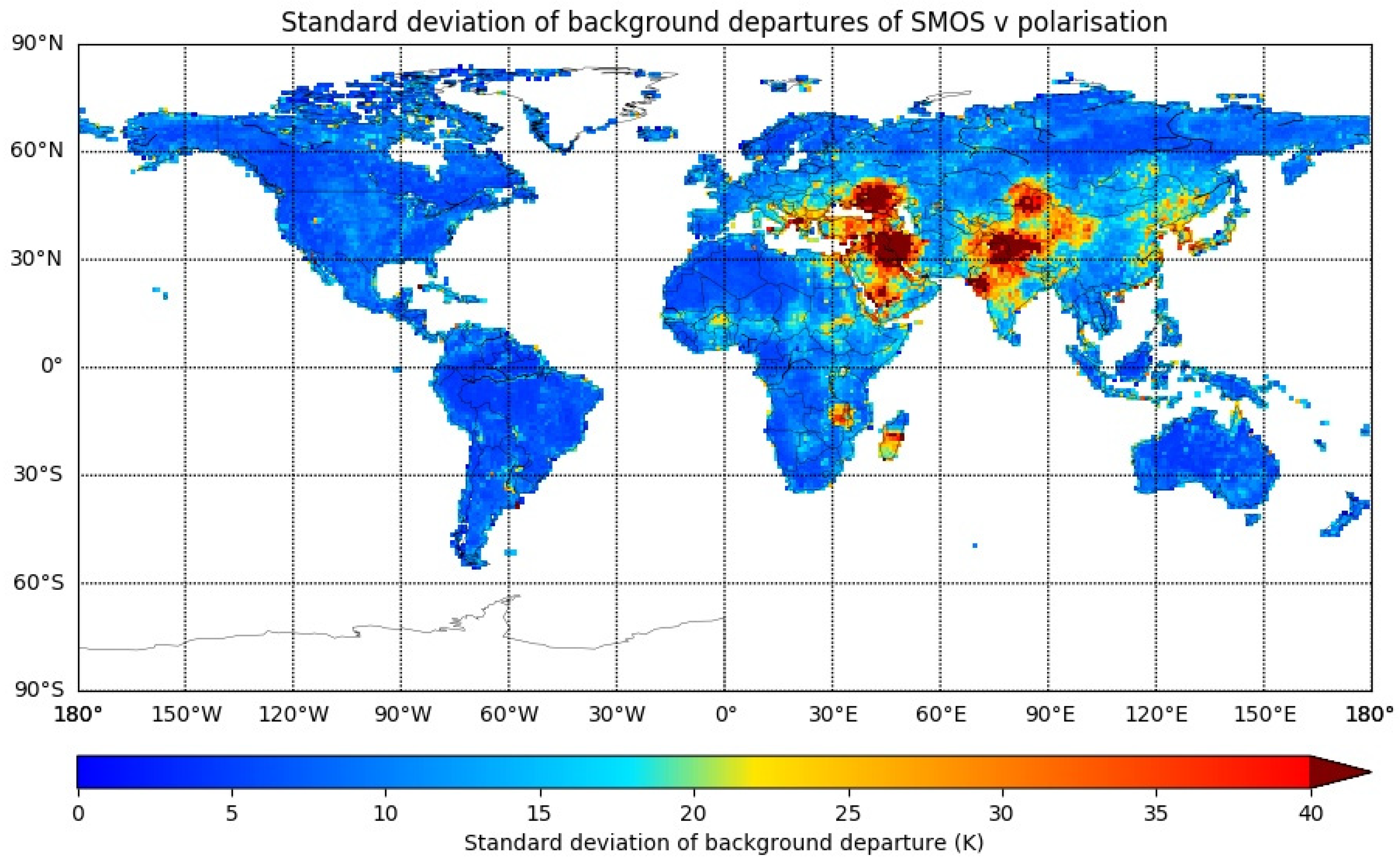
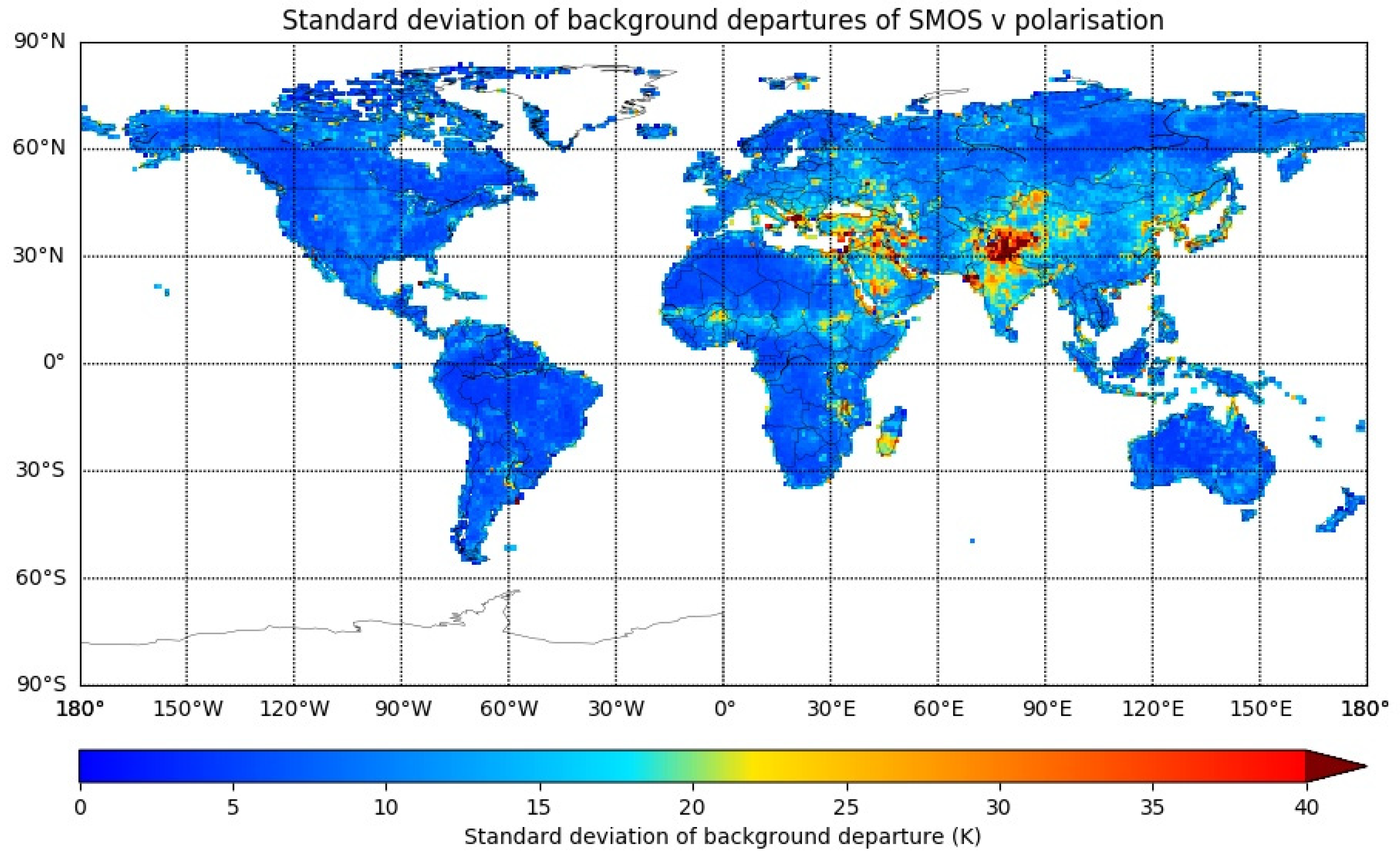
If bit number 1 of the SMOS information flags in the SMOS input BUFR files is set, this indicates that radio frequency interference (RFI) is present in the data, and any observations with this bit set are not processed any further. However, this RFI flagging used in the SMOS monitoring is inadequate and fails to correctly screen out many observations which are obviously contaminated by RFI. This can clearly be seen with the increased background departures (after screening), particularly over the Middle East and northern India in Figure 1.

Table 1 shows that there are two additional RFI flags (bit numbers 4 and 9) that are not used. Bit number 1 identifies observations that are directly affected by RFI sources. Bit number 4 identifies observations that are indirectly affected by the tails of the RFI sources or via the sidelobes of the instrument impulse response. Bit number 9 identifies observations affected by RFI via a long-term trend analysis. Results from additionally using the other two RFI flags are shown in Section 3.2.1.

2.1.2. Alias-Free Zone

In addition, bit number 5 indicates that data is from the alias-free zone of the SMOS snapshot, and only data with this bit set are passed to the monitoring system. Any observations without bit number 5 set are removed in the pre-screening, which means only SMOS observations in the alias-free zone are monitored.

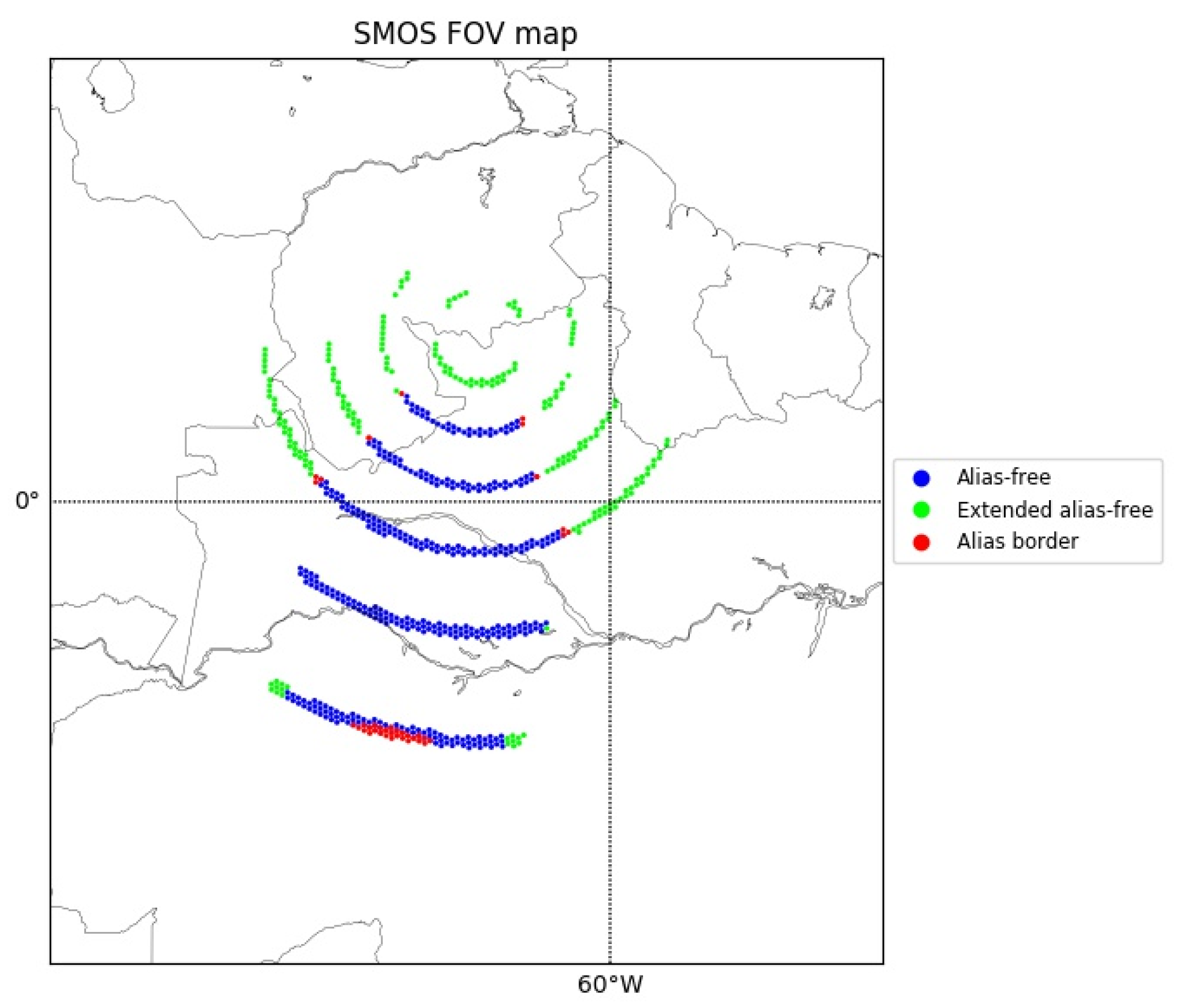
Figure 2 shows a SMOS snapshot with observations in the alias-free zone in blue, observations in the extended alias-free zone in green, and observations in the border between the two in red. The separate rings of observations contain SMOS observations at different incidence angle bins from 10° to 60° at 10° intervals.

See Section 3.2.2 for the results of relaxing the check on bit number 5 and additionally monitoring observations in the extended alias-free zone.

2.1.3. Additional Flags

Table 1 shows that there are many additional flags that are not used. These could be used to refine the sample of SMOS observations that are monitored. Some of those that could be used in the future are discussed in Section 3.2.3.

2.2. Model-Based Quality Control

After the pre-screening, the remaining SMOS observations are read into the IFS, and further screening procedures are undertaken to avoid areas where the observations cannot be accurately modelled by CMEM. These are summarised in

Table 2. Quality control applied to SMOS observations within the IFS.

Screening Reason	Threshold for Rejection
Extreme values	Measured Tb less than 50 K or greater than 340 K
Snow	Model snow depth greater than 1cm
Frozen surfaces	Model 2 metre air temperature less than 273 K

. The extreme value check is aimed at screening out SMOS observations that have unphysical Tb values due to instrument anomalies or undetected RFI. The snow and frozen surface checks are aimed at screening out SMOS observations in areas where the quality of the forward modelling is sub-optimal, which would result in large background departures contaminating the global statistics. In addition to the checks in Table 2, each observation location is classified as land if the model land-ocean mask value in the collocated grid point is greater than 0.5 and classified as ocean otherwise. The procedures in Table 2 are performed for observations over both land and ocean, but it would be possible to implement different quality control procedures depending on whether the observation is over land or ocean if deemed necessary.

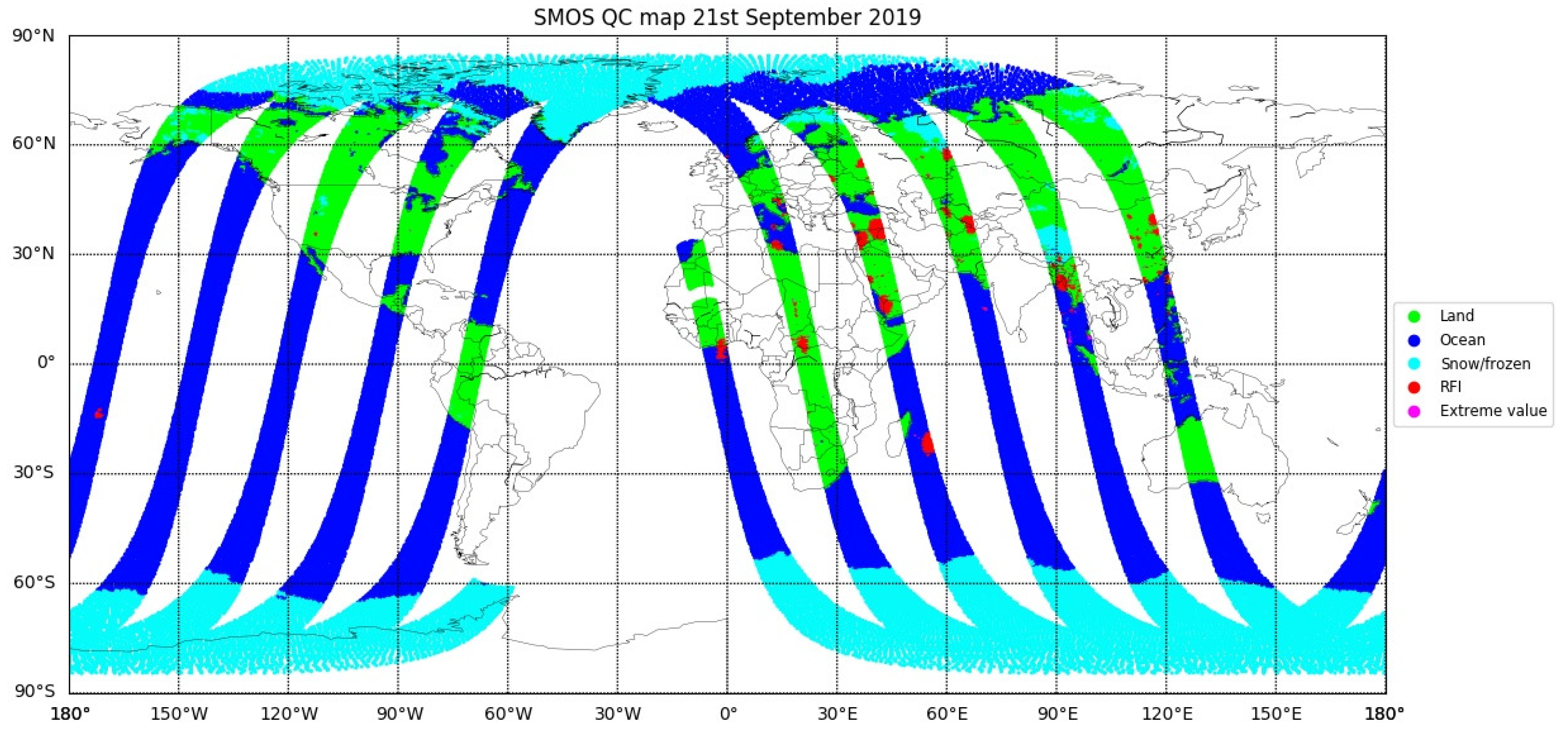
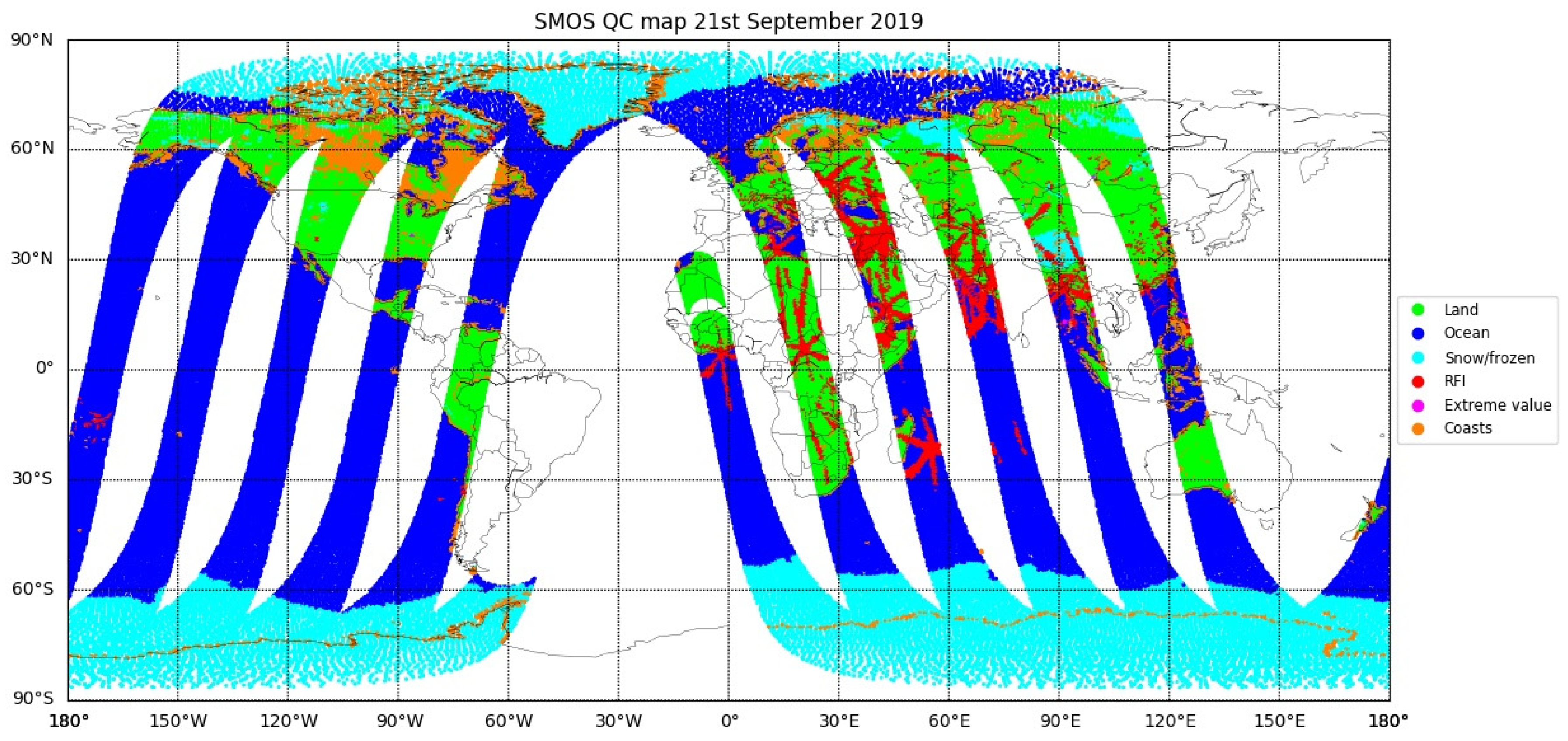
Figure 3 shows the geographical distribution of the surface type and quality control applied. Most observations over the poles and at high latitudes are screened out by the snow and frozen surface checks, including some areas covered by sea ice. There are RFI detections, i.e., observations flagged by only bit number 1 from Table 1, over the Middle East, Eastern Europe and parts of Asia. Very few observations are screened out by the simple extreme value check.

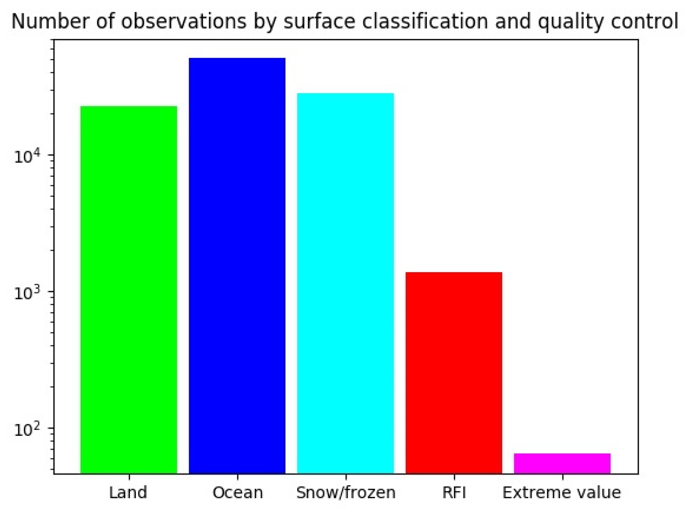
Figure 4 provides a breakdown of typical numbers of observations during a 12 h period, which are classified as land or ocean, and also the numbers of observations screened out by the checks detailed in Table 2. The check which screens out the most observations is the snow/frozen surfaces check, and this number increases further in the northern hemisphere winter when snow covers much of Canada, Northern Europe and Russia. RFI accounts for the next most observations to be screened out, and finally, the extreme value check accounts for the least.

2.2.1. Land-Ocean Classification

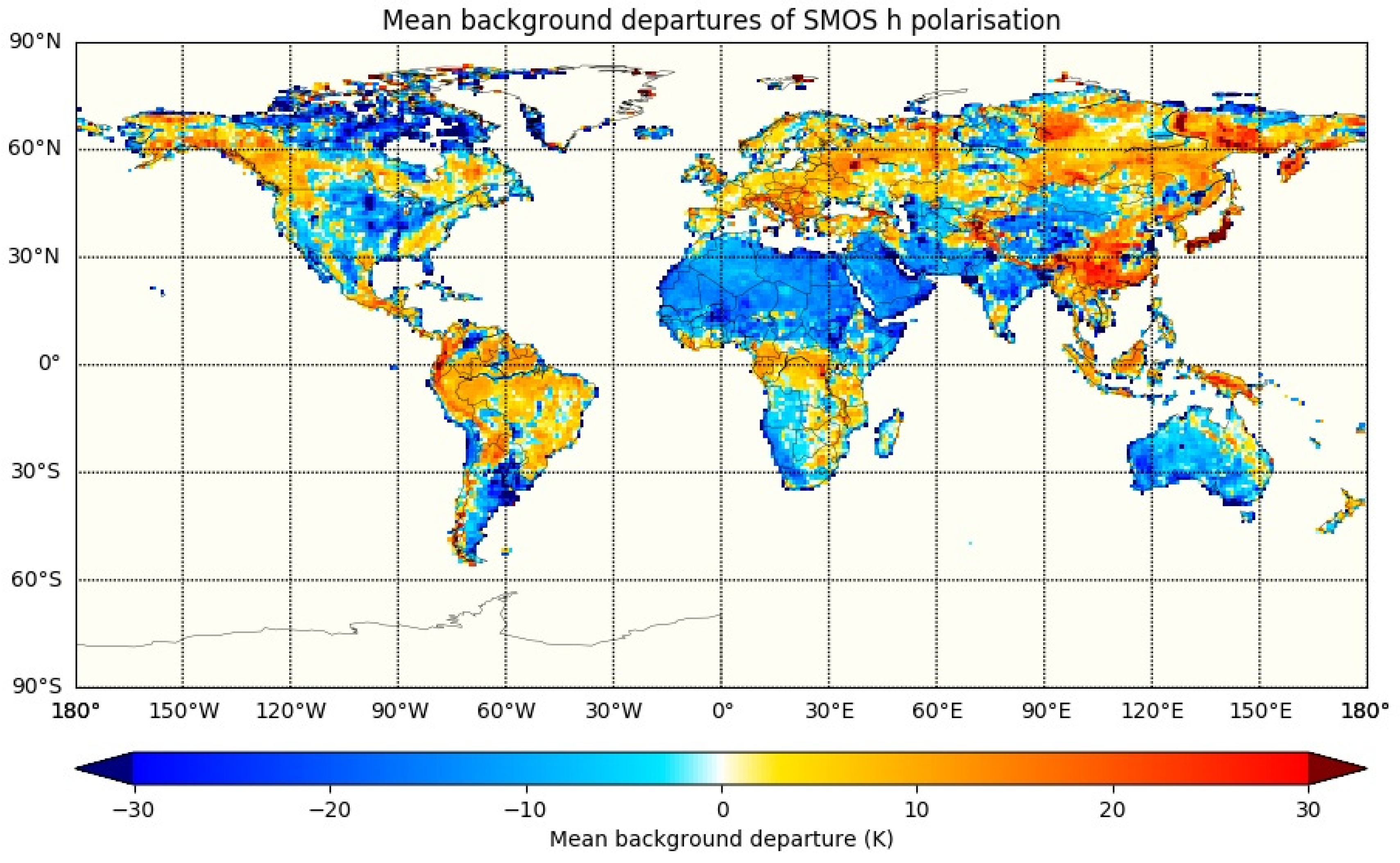
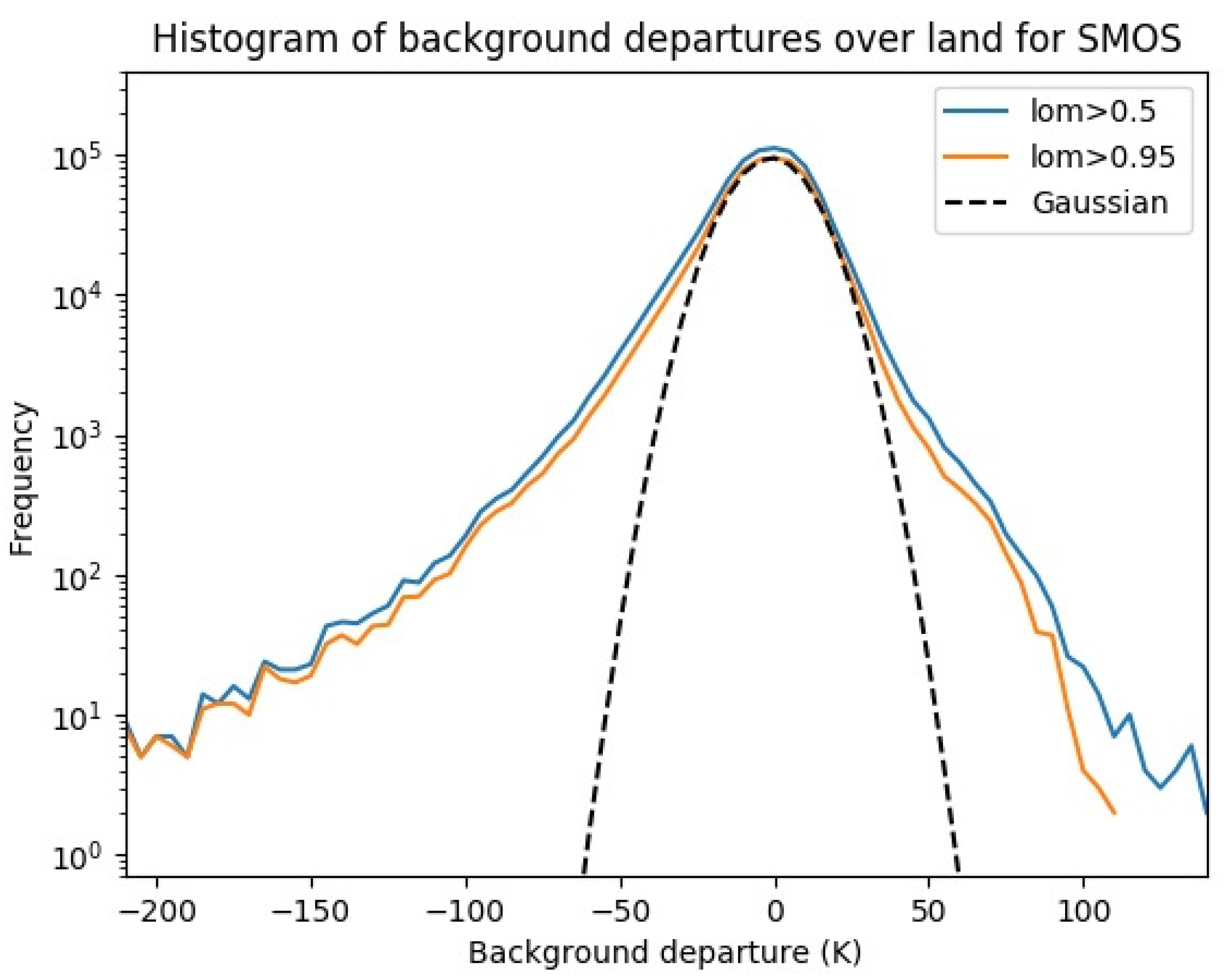
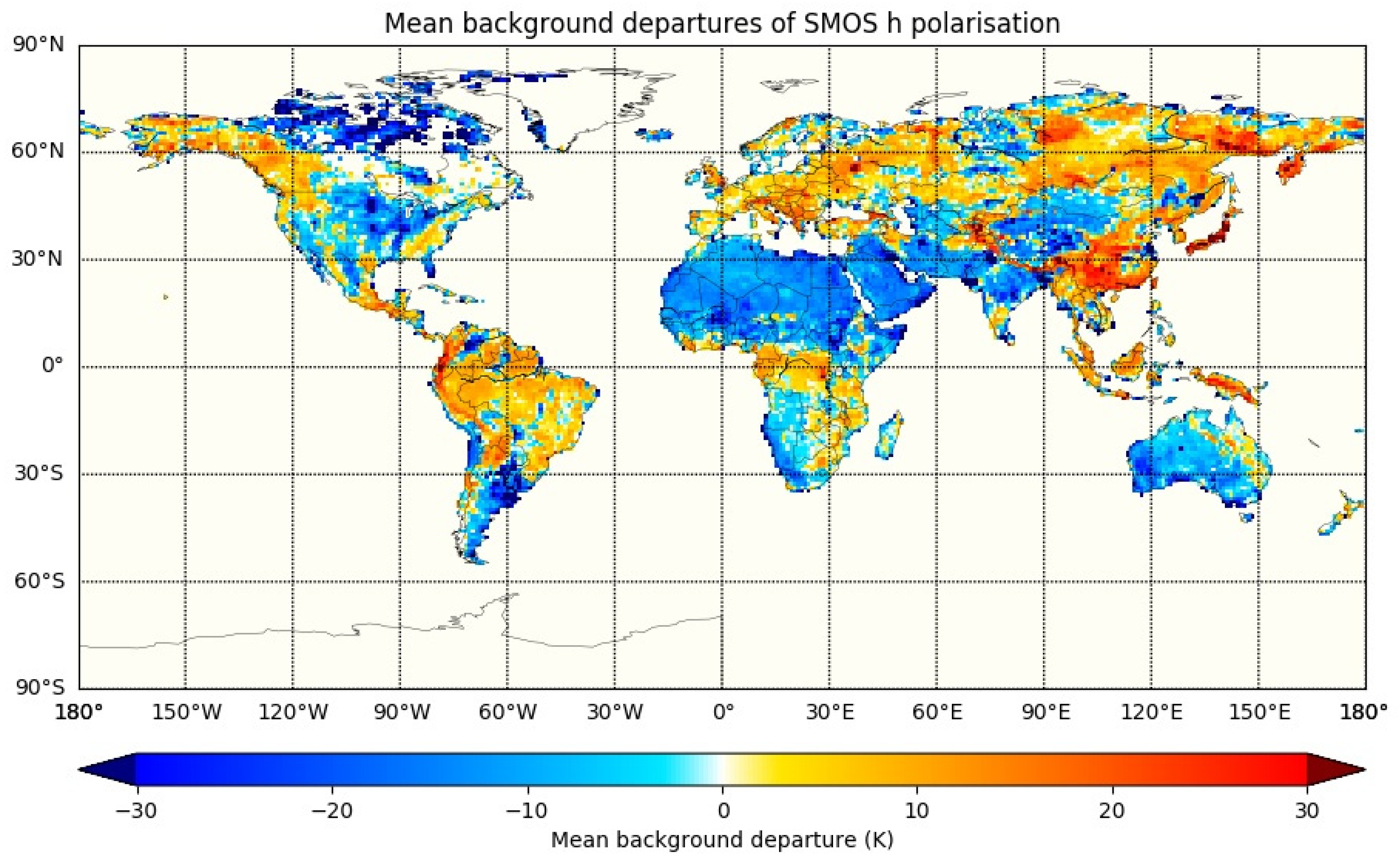
Observations are classified as over land or over ocean based on how much of the closest model grid box is covered by land. If more than 50% of the model grid box is covered by land, then the observation is classified as over land; otherwise, it is classified as over ocean. This means many coastal areas and regions close to lake edges are considered to be over land. As seen in Figure 5, the mean background departures are generally larger over coasts and lakes, which contribute to large tails in the overall distribution of the background departures. This is due to CMEM’s binary response to whether an observation is over land or ocean and not accounting for mixed land and ocean (or lake) points. For further discussion of this, see Section 3.3.1 and Section 4.

For assimilation of observations, a Gaussian (thus symmetric) distribution is assumed. Therefore, to enable assimilation, better screening for coasts are needed. For the assimilation of microwave radiances in the atmosphere, a model grid box must be covered by greater than 95% land to be considered over land [6]. So, a more consistent coastal screening for SMOS would be to classify the surface type as follows. If a model grid box is covered by:

• less than 1% land it is classified as over ocean;
• between 1% and 95% land it is classified as coast and screened out;
• over 95% land it is classified as over land.

Results when using this screening method are shown in Section 3.3.1.

2.2.2. Sea Ice Screening

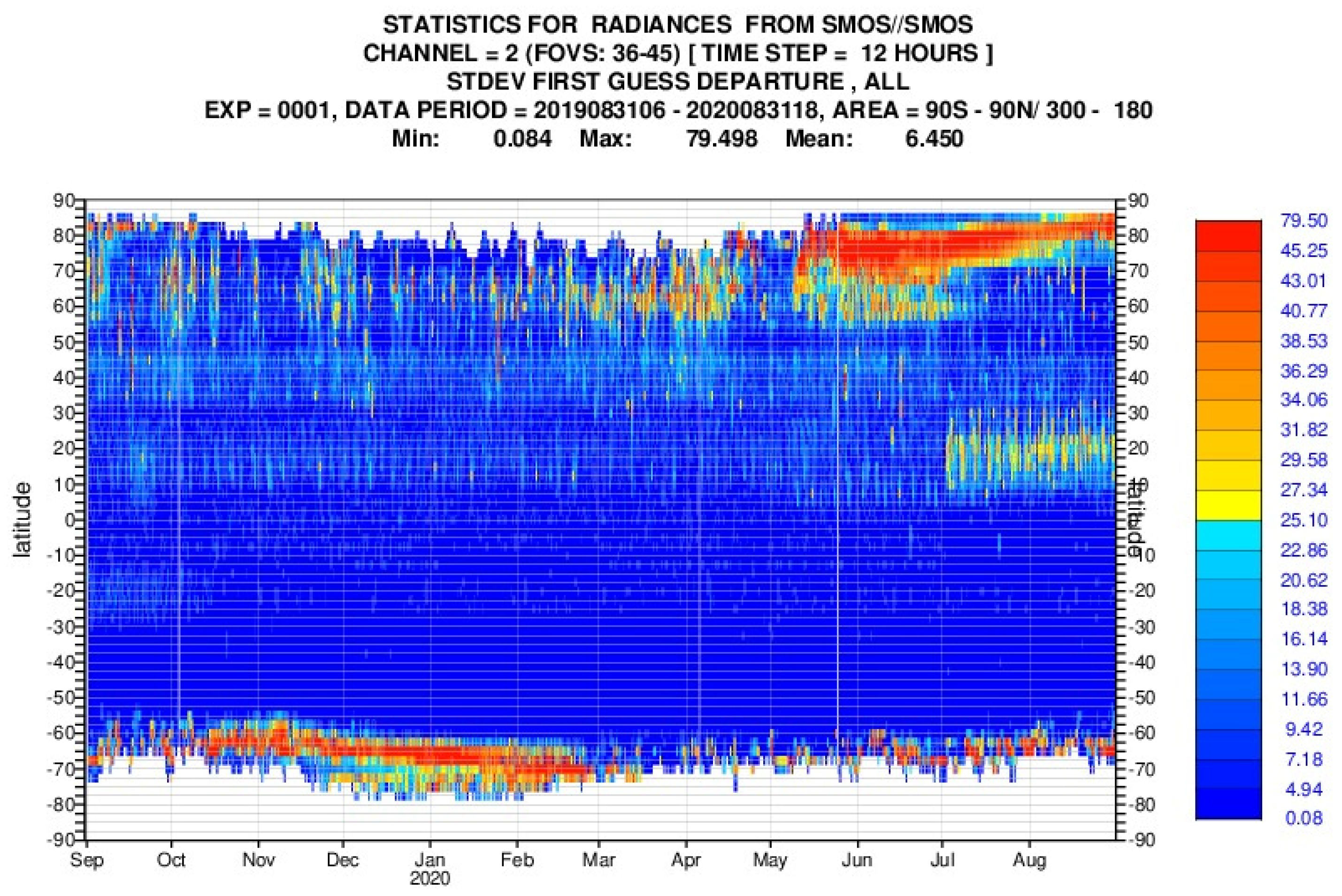
In late May and early June 2020, there was a significant increase in the mean and standard deviation of background departures over ocean in the area between 70 °N and 80 °N, see Figure 6. A similar increase can be seen between 60 °S and 70 °S between October 2019 and March 2020. The time of the change coincides with a period of intense melting of Arctic/Antarctic sea ice. Therefore, it seems that the cause of the change in the statistics was that the frozen surface screening was not correctly flagging data in these areas at these times.

As shown in Table 2, the frozen surface screening applied in the IFS consisted of a check on whether the 2 m temperature is less than 273 K and whether the snow depth is greater than 1 cm. The areas affected in May/June 2020 were over ocean, so the snow depth check would not be considered, and the 2 m air temperature was greater than 273 K, so the current frozen surface screening does not flag the observations in these areas. However, there is still sea ice present. Hence, background departures for SMOS observations over sea ice are calculated. Currently, CMEM does not contain a model for calculating the emissivity over sea ice, so it assumes the observations are over ocean. The radiative emissivity over sea ice and open ocean at L-band is significantly different, leading to a large discrepancy between the measured Tbs over sea ice and the simulated Tbs assumed to be over ocean, causing the increased background departures.

A potential solution to this issue is to additionally perform a check on the model sea ice concentration directly. This is also done to assimilate MW radiances into the atmospheric model and avoids the use of surface-sensitive observations over sea ice where the radiative transfer modelling is not as accurate as over open ocean. See Section 3.3.2 for the results of implementing such an additional check.

3. Results

3.1. Experiment Setup

Table 3. Description of experiments run to test the SMOS quality control enhancements.

Experiment ID	Description
CTRL	Control (baseline quality control as described in Section 2)
RFI_EXP	CTRL + using RFI flags in bit numbers 4 and 9
EAF-FOV	CTRL + monitoring observations in the extended alias-free zone (relaxing the check on bit number 5)
ICE	CTRL + screening out observations where the model sea ice concentration is greater than 0.01 (1%)
COASTS	CTRL + screening out observation whose nearest model grid point has a land-ocean mask value between 0.01 and 0.95 (1% and 95%)
COMBI	CTRL + all of the changes combined

shows the experiments which were performed to test the enhancements to the various quality control procedures outlined in Section 2. All experiments were run for a month in summer 2019 between 16 June and 15 July 2019 using version 6.20 of the SMOS L1C Brightness Temperature product. The IFS is configured to use model cycle 47r1 (https://www.ecmwf.int/en/forecasts/about-our-forecasts/evolution-ifs/cycles/summary-cycle-47r1, accessed on 11 October 2021) which was operational between 30 June 2020 and 11 May 2021, and the model resolution was T_L399 (approximately 50 km grid spacing). Each experiment used identical background forecasts and SMOS observations as inputs, and only the quality control procedures were changed between the different experiments.

3.2. Observation-Based Quality Control

3.2.1. Radio Frequency Interference (RFI)

As shown in Section 2.1.1, the operational RFI screening used in 2019 was sub-optimal and missed screening out many SMOS observations, which are clearly affected by RFI. It only used the RFI flag in bit number 1 of the SMOS BUFR flag table [5]. However, there are additional flags in bit numbers 4 and 9 provided with the SMOS observations, which can be used to more effectively screen out RFI. The RFI_EXP experiment has been run to test the use of these additional RFI flags.

Comparing Figure 1; Figure 7 shows that many of the areas of increased background departures have reduced, particularly over the Middle East. However, even with the new screening, there are still areas of increased background departures in areas of known RFI sources (e.g., Northern India) which shows that this screening is still not perfect.

From September 2020 onwards, the additional flags are included in the operational screening, and separate plots with the screening turned on and off are now available on the monitoring web page.

3.2.2. Extended Alias-Free Zone

The EAF-FOV experiment has been run to extend the monitoring to include observations from the extended alias-free zone by relaxing the existing check on bit number 5 of the NRT BUFR product within the pre-screening. The information on whether a given observation is in the alias-free zone or not is retained, and then background departure statistics have been calculated separately for those observations within the alias-free zone and those in the extended alias-free zone.

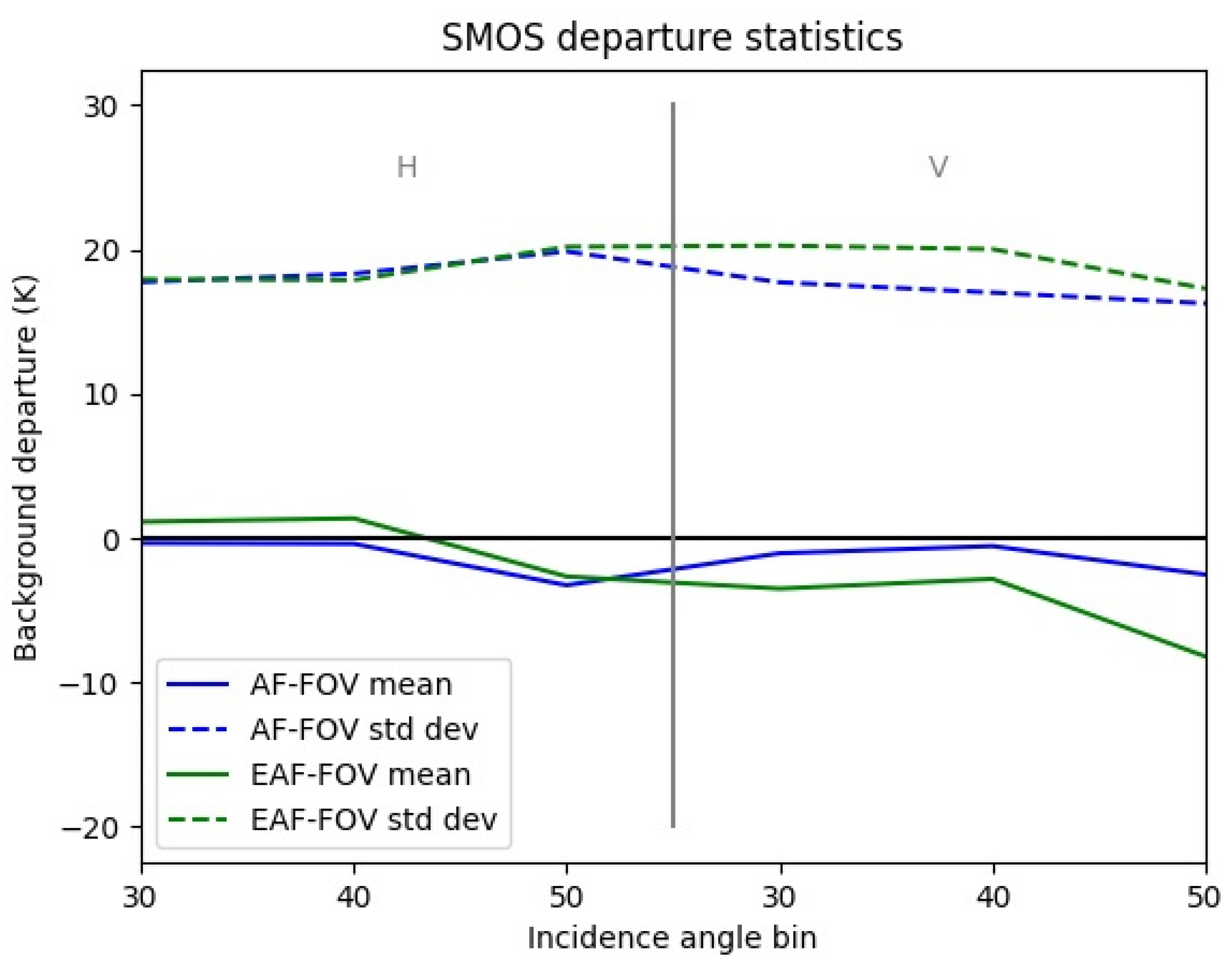
Figure 8 shows that the background departure statistics are comparable for observations in the alias-free and extended alias-free zones. For the H polarisation, the background departure statistics are almost identical. For the V polarisation, the mean background departures are slightly more negative, and the standard deviation of background departures are slightly higher for the extended alias-free zone. It should be noted that, as illustrated in Figure 2, there are very few observations in the extended alias-free zone with incidence angles around 50 degrees which means the statistics presented in Figure 8 for this incidence angle bin are from a very small sample. The benefit of additionally monitoring observations in the extended alias-free zone is enhanced spatial and temporal coverage of the monitored observations.

3.2.3. Additional Flags

Table 1 shows that there are many other flags associated with the SMOS observations, mostly related to solar and lunar effects on the data. Using the CTRL experiment, the effects that these flags have on the data quality has been studied to assess whether observations with any of these flags set should additionally be screened out.

A preliminary analysis of the background departure statistics from samples formed with different combinations of these flags set is shown in

Table 4. Summary of number of observations and background departure statistics for samples of SMOS observations separated by different combinations of quality control flags set. Note that in all these observations, bit numbers 5 and 13 were set, indicating the observations are in the alias-free zone and that a direct sun correction was applied. Also, bit numbers 1, 4, and 9 were not set, indicating these observations were free of RFI. Data is accumulated between 16 June 2019 and 15 July 2019.

Bit 2 (Sun tails)	Bit 3 (Alias Border)	Bit 6 (Moon Alias)	Bit 7 (Sun Reflection)	Bit 11 (Moon Correction)	Count	Mean Background Departure (K)	Standard Deviation Background Departure (K)
0	0	0	0	0	153,630	−0.79	16.83
1	0	0	0	0	28,419	−0.21	16.46
0	1	0	0	0	22,921	−1.72	17.47
1	1	0	0	0	1917	−0.36	17.24
0	0	0	1	0	1	−50.55	N/A
1	1	0	1	0	1	−66.72	N/A
0	0	0	0	1	426,025	−0.52	17.14
1	0	0	0	1	83,411	0.19	16.98
0	1	0	0	1	59,239	−1.40	17.95
1	1	0	0	1	10,656	−0.24	16.95
0	1	1	0	1	18	−7.44	17.44
0	0	0	1	1	30	−6.65	36.32
0	1	0	1	1	14	−2.04	31.13
1	1	0	1	1	14	−43.66	51.18

. The results indicate that bit numbers 2 and 3 have a small effect on the background departure statistics, with the majority of observations having neither of these bits set. Bit number 11 (indicating a moon correction has been applied to the data) is set for the majority of observations but also has a negligible effect on the background departure statistics. However, bit number 7 (indicating solar reflection) does have a very large effect on the background departures and indicates that observations with this bit set have a significantly larger mean and standard deviation of background departures, indicating degraded data quality. This suggests that it would be beneficial to screen out observations with bit number 7 set. Bit number 6 is only set for 18 observations in the period, and bits 8, 10 and 12 were not set in any of the observations. Therefore, to investigate the effect of these flags on background departure statistics would require different or larger samples to be analysed, which will be the subject of future work.

3.3. Model-Based Quality Control

3.3.1. Coastal Screening

The COASTS experiment has been run to test the classification of observations over land using a threshold on the model land-ocean mask value of 95% instead of 50%. Figure 9 shows that this change reduces the tails of the distribution and makes the distribution more Gaussian and symmetric, especially near the centre. However, even with the more conservative coastal screening, the distribution is still biased negative due to other error sources such as RFI and missed frozen surfaces. For example, the observed Tb may be significantly smaller than the simulated background Tb where there is RFI affecting the sidelobes of the instrument impulse response. Alternatively, where there is no snow in the model, but there is in reality, the observed Tb will be colder than the background simulated Tb.

In addition, Figure 10 shows a reduction in the large biases surrounding the coasts, which are shown in Figure 5. The clearest differences can be seen around the islands in Northern Canada, Northern Europe and the maritime continent. There are still significant local biases in inland areas, but the larger biases in coastal and mixed land-ocean-lake areas have been successfully removed by the new coastal screening.

3.3.2. Sea Ice Screening

As shown in Section 2.2.2, the baseline frozen surface screening did not perform well over ocean during the 2020 melt season. This is because the baseline screening tests on whether there is a snow depth of greater than 1cm or if the 2 m temperature is greater than 273 K. Over land, this seems to perform adequately, but over ocean, there are large areas where observations over sea ice are allowed through and into the monitoring system.

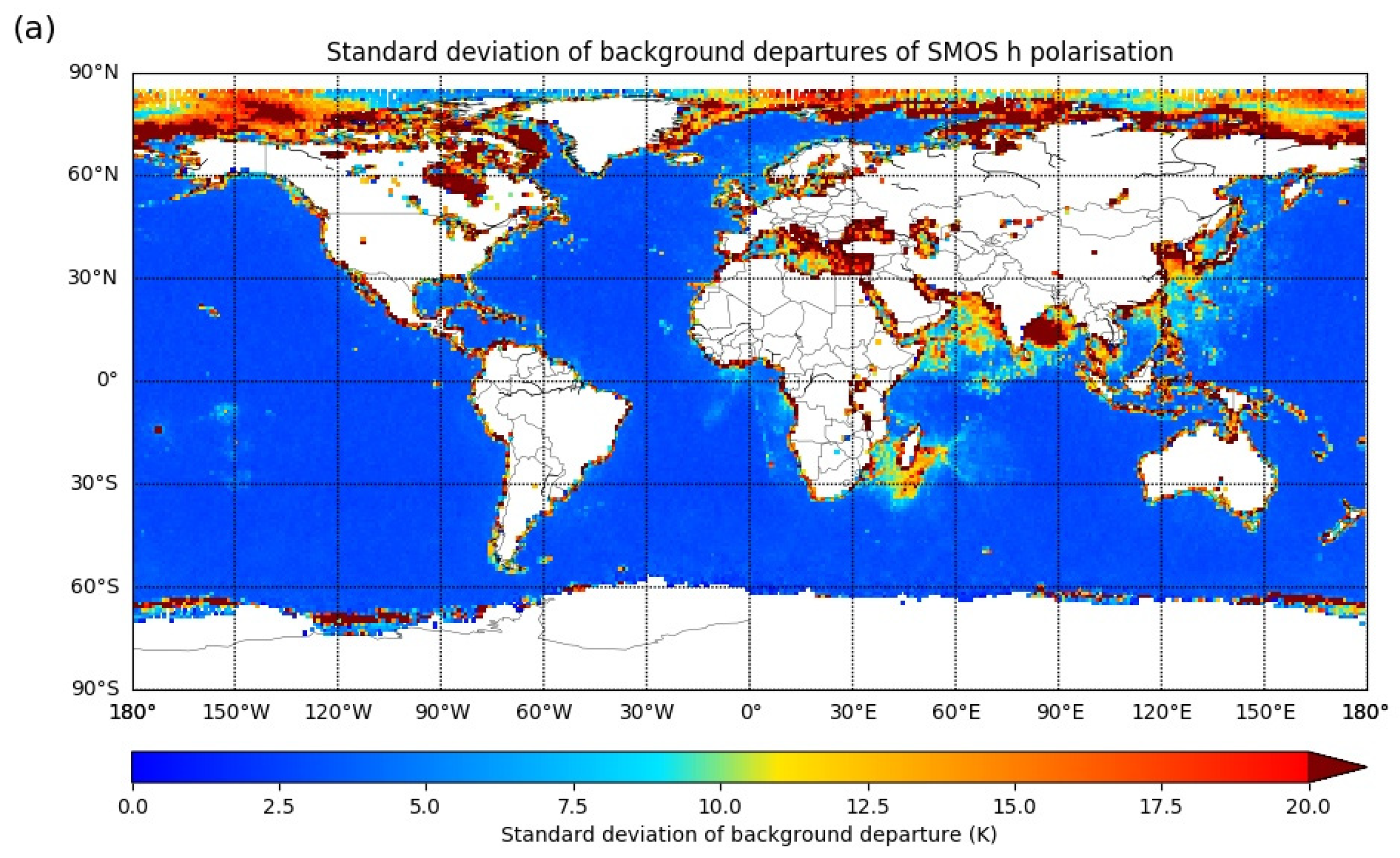
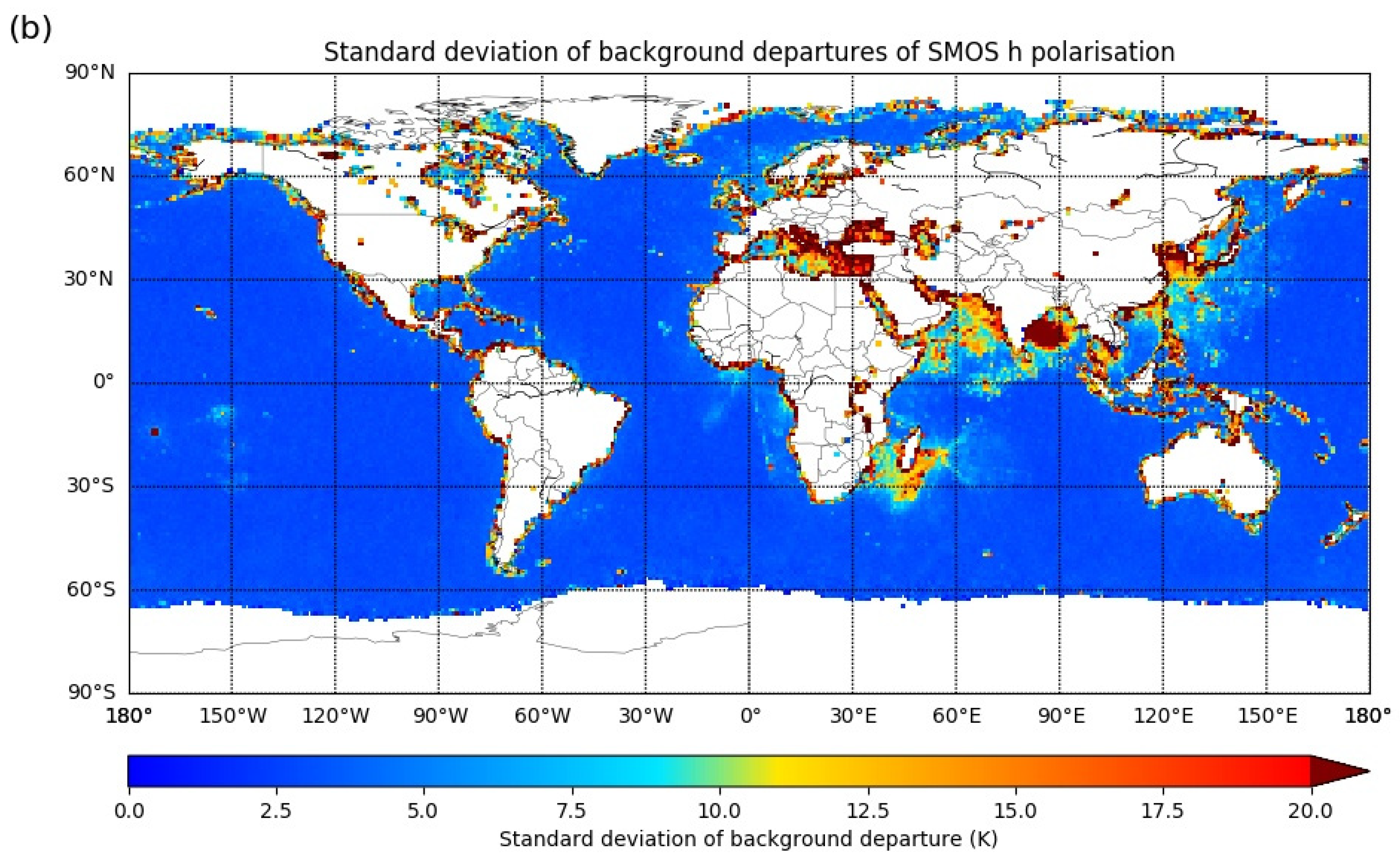
As introduced in Section 2.2.2, an improved frozen surface screening with an additional check on whether the model sea ice concentration is greater than 0.01 has been implemented and tested in the ICE experiment. Figure 11 shows that the areas of larger background departures over the North pole and Arctic Ocean (and around the sea ice edge in the Southern Ocean) in the CTRL experiment are removed in the ICE experiment for SMOS observations with V polarisation (the same effect is seen for H polarisation, not shown). This indicates that the new screening successfully removes observations where the 2-metre temperature is above 273K, but there is sea ice present.

3.4. Combined Results

As shown in Section 3.2 and Section 3.3, the experiments testing different quality control changes separately show good results and solve many of the problems associated with the baseline quality control procedures identified in Section 2. Therefore, the COMBI experiment has been run, which combines the RFI, extended alias-free zone, additional flags, coastal, and sea ice screening changes together.

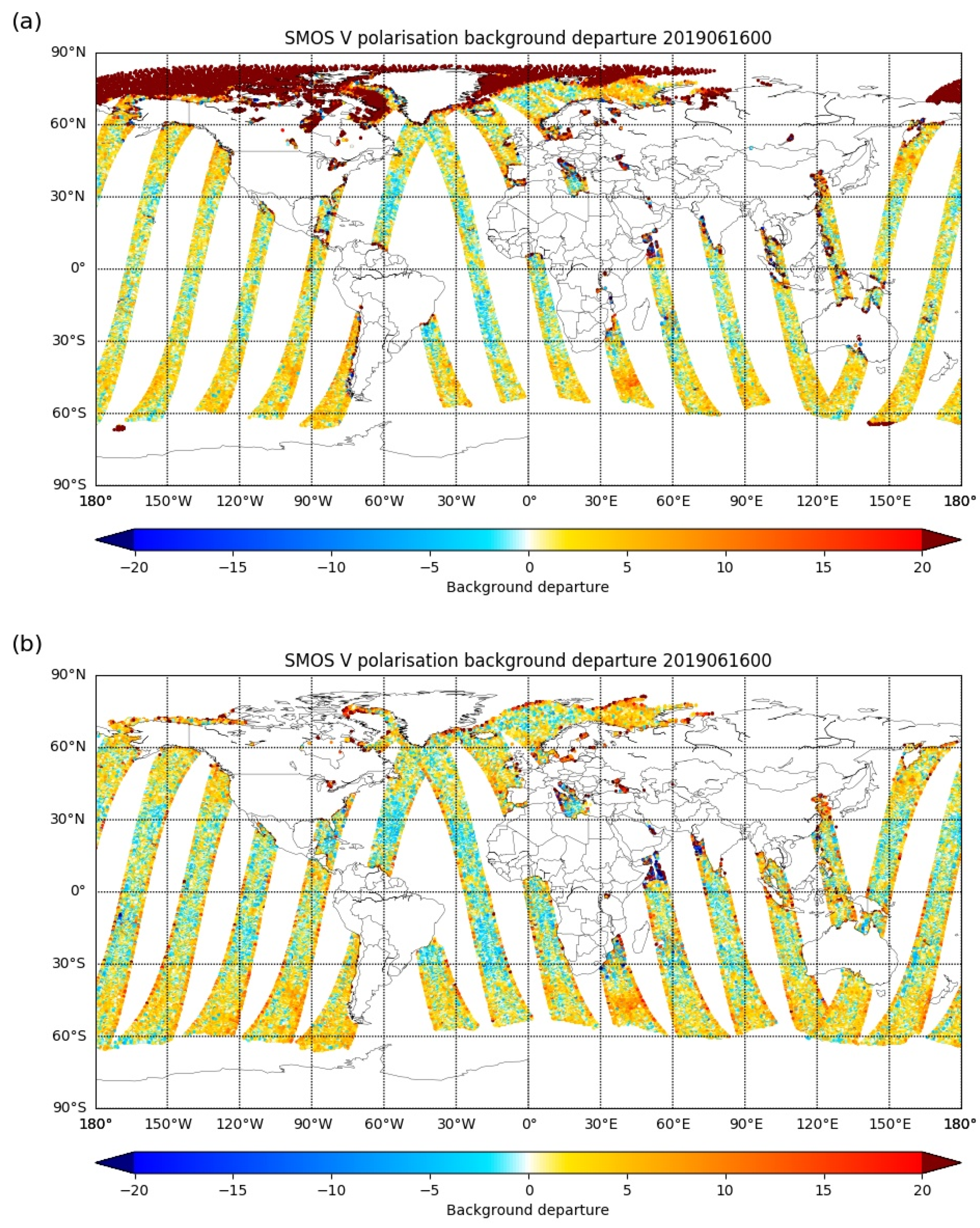
Figure 12 shows a snapshot of those observations which pass quality control in the CTRL and COMBI experiments. The clearest difference is the removal of the positively biased observations over the northern polar regions due to the enhanced sea ice screening. Other notable features are the wider swaths due to the additional extended alias-free zone observations and the removal of some of the observations with larger background departures surrounding the coasts (e.g., the western coast of South America) and inland lakes (e.g., in Northern Canada).

Figure 13 is the equivalent of Figure 3, showing the additional areas which are screened out in the COMBI experiment compared to the CTRL experiment. The most notable features are the observations screened by the new coastal screening, which, as well as surrounding the coasts, extend far inland over the lakes of Northern Canada and Scandinavia. Also, there are many more observations screened out by the RFI checks due to the use of the additional RFI flags. The wider swaths from the additional extended alias-free zone observations can also be seen. The sea ice change is more subtle because the data chosen in September does not coincide with a melt season in either the Northern or Southern polar regions.

Table 5. Global statistics for different surface types, polarisations and incidence angles for the SMOS observations passing quality control in the CTRL and COMBI experiments. Data is accumulated between 16 June 2019 and 15 July 2019.

Experiment			CTRL			COMBI
Surface	Polarisation	Incidence Angle	Count	Mean Background Departure (K)	Stdev Background Departure (K)	Count	Mean Background Departure (K)	Stdev Background Departure (K)
Land	H	30	813,630	−0.56873	17.82601	998,443	0.556094	15.62785
	H	40	1,150,296	−0.39031	18.36825	1,372,871	0.612522	16.06992
	H	50	1,127,649	−3.17983	19.90534	875,275	−3.12986	17.97185
	V	30	811,544	−0.89444	17.85482	959,740	−1.33494	14.91334
	V	40	1,144,818	−0.52727	17.10982	1,311,434	−0.65819	14.16749
	V	50	1,117,124	−2.7916	16.36671	819,610	−2.07995	11.97337
Ocean	H	30	1,943,327	13.42583	30.78681	2,633,329	3.73329	5.371872
	H	40	2,851,385	14.46067	31.43319	3,714,355	4.910848	5.467572
	H	50	2,834,376	15.8351	31.30319	2,477,014	5.963169	5.149798
	V	30	1,943,957	11.10171	29.69314	2,654,302	1.349128	5.292711
	V	40	2,854,129	11.73128	28.80636	3,734,606	2.686217	5.447312
	V	50	2,837,617	11.26956	26.32029	2,469,972	2.820669	5.124058

shows that the combined changes to the quality control procedures result in significant changes to the global background departure statistics and number of observations monitored. For incidence angles of 30 and 40 degrees, there are significantly more observations monitored, with the increase from the additional extended alias-free zone observations outweighing the decreases from the RFI, sea ice, and coastal screening. For incidence angles of 50 degrees, there are fewer observations monitored because at this incidence angle, there are not many additional observations in the extended alias-free zone (see the second most outer ring of observations in Figure 2), so the decreases from the other quality control changes dominate. Over land, there are small changes to the mean background departures but significant reductions to the standard deviation of background departures. This is mostly due to the additional RFI screening, as shown when comparing Figure 7; Figure 1. Over ocean, there are large reductions to both the mean and standard deviation of background departures, which is mainly due to the additional sea ice screening as illustrated in Figure 11.

Considering these results, the enhanced SMOS quality control procedures presented in this paper were implemented with the most recent ECMWF cycle upgrade, 47r2, and are effective from 11 May 2021 onwards.

4. Conclusions

The various changes to quality control procedures have different effects on the background departure statistics and number of observations monitored. Generally, the effects are positive by including more observations in the monitoring (e.g., extended alias-free zone), reducing mean background departures (e.g., coastal screening), and reducing the standard deviation of background departures (e.g., RFI screening). Over ocean, there are striking improvements in the global background departure statistics from the additional sea ice screening. In a monitoring context, this means that smaller changes in data quality will be detectable as the global background departure statistics will not be contaminated by observations in gross disagreement with their model equivalents.

There are various further enhancements that could be made to the quality control of SMOS data. As shown in Figure 7, the RFI screening is still not perfect, and it is clear that RFI contaminated observations are still passing the updated quality control. Ongoing activities are aiming to address this by developing a new ground-based RFI detection system (GRDS) which aims to screen out RFI-affected data more effectively using various statistical algorithms [7]. Initial results from this system indicate that it is a significant improvement on the baseline screening, and future work will involve adapting the system for operational use as part of the SMOS ground segment [8].

In addition, there is ongoing work at ECMWF to improve the sea ice and coastal screening in other MW radiance observations, which could be applied to SMOS data in the future. In particular, the use of FASTEM [9] as part of the RTTOV [10] radiative transfer model to calculate surface emissivities over ocean could be used to produce more realistic and accurate simulated Tbs for SMOS over ocean. In coastal areas, a weighted average of the FASTEM/RTTOV simulated Tb, and the CMEM simulated Tb using the fraction land-ocean mask information could be used. This has the potential to significantly improve the quality of the background departures in coastal regions and could lead to the relaxation of the coastal screening documented in Section 3.3.1. There is also ongoing work to improve the performance of CMEM over snow-covered areas [11], which could be extended to sea ice areas too.

In parallel to the developments to the SMOS monitoring documented in this paper, the monitoring of L-band observations from the NASA SMAP [12] instrument has been implemented in the IFS. The SMAP monitoring went online on 11 May 2021. This has enabled comparisons between SMOS and SMAP to be analysed, as well as opening possibilities for full exploitation of passive L-band data in the IFS.

Finally, the long-term aim of improving the quality control of observations is to enable the effective assimilation of those observations. This is no different for SMOS, and the quality control improvements made here should facilitate improved results compared to previous attempts to directly assimilate SMOS Tbs into the ECMWF land data assimilation system (LDAS) [13]. This will be the subject of future work.

References

- Kerr, Y.H.; Waldteufel, P.; Wigneron, J.-P.; Delwart, S.; Cabot, F.; Boutin, J.; Escorihuela, M.-J.; Font, J.; Reul, N.; Gruhier, C.; et al. The SMOS Mission: New Tool for Monitoring Key Elements of the Global Water Cycle. Proc. IEEE 2010, 98, 666–687. [Google Scholar] [CrossRef] [Green Version]
- De Rosnay, P.; Drusch, M.; Boone, A.; Balsamo, G.; Decharme, B.; Harris, P.; Kerr, Y.; Pellarin, T.; Polcher, J.; Wigneron, J.-P. AMMA Land Surface Model Intercomparison Experiment coupled to the Community Microwave Emission Model: ALMIP-MEM. J. Geophys. Res. Space Phys. 2009, 114. [Google Scholar] [CrossRef]
- Sabater, J.M.; Fouilloux, A.; De Rosnay, P. Technical implementation of SMOS data in the ECMWF Integrated Forecasting System. IEEE Geosci. Remote. Sens. Lett. 2012, 9, 252–256. [Google Scholar] [CrossRef]
- De Rosnay, P.; Muñoz-Sabater, J.; Albergel, C.; Isaksen, L.; English, S.; Drusch, M.; Wigneron, J.-P. SMOS brightness temperature forward modelling and long term monitoring at ECMWF. Remote. Sens. Environ. 2020, 237, 111424. [Google Scholar] [CrossRef]
- De Rosnay, P.; Dragosavac, M.; Drusch, M.; Gutiérrez, A.; Rodríguez López, M.; Wright, N.; Muñoz Sabater, J.; Crapolicchio, R. SMOS NRT BUFR Specification. 2015. Available online: https://earth.esa.int/documents/10174/1854583/SMOS_NRT_BUFR_Specification (accessed on 11 October 2021).
- Weston, P.; Bormann, N.; Geer, A.J.; Lawrence, H. Harmonisation of the Usage of Microwave Sounder Data over Land, Coasts, Sea Ice and Snow: First Year Report. No. 45. ECMWF Fellowship Programme Research Report. 2017. Available online: https://www.ecmwf.int/node/17766 (accessed on 10 October 2021).
- Oliva, R.; Martellucci, A.; Daganzo-Eusebio, E.; Jorge, F.; Soldo, Y.; English, S.; De Rosnay, P.; Weston, P.; Barbosa, J.; Nestoras, I. Results from the ground RFI detection system for passive microwave Earth observation data. In Proceedings of the Virtual Meeting (IGARSS 2021), Brussels, Belgium, 12–16 July 2021. [Google Scholar]
- Weston, P.; de Rosnay, P.; English, S. GRDS Test-Bed Report. 2021. Available online: https://0-doi-org.brum.beds.ac.uk/10.21957/8kv6wj087 (accessed on 10 October 2021).
- Liu, Q.; Weng, F.; English, S.J. An improved fast microwave water emissivity model. IEEE Trans. Geosci. Remote Sens. 2010, 49, 1238–1250. [Google Scholar] [CrossRef]
- Saunders, R.; Hocking, J.; Turner, E.; Rayer, P.; Rundle, D.; Brunel, P.; Vidot, J.; Roquet, P.; Matricardi, M.; Geer, A.; et al. An update on the RTTOV fast radiative transfer model (currently at version 12). Geosci. Model Dev. 2018, 11, 2717–2737. [Google Scholar] [CrossRef] [Green Version]
- Hirahara, Y.; de Rosnay, P.; Arduini, G. Evaluation of a Microwave Emissivity Module for Snow Covered Area with CMEM in the ECMWF Integrated Forecasting System. Remote Sens. 2020, 12, 2946. [Google Scholar] [CrossRef]
- Entekhabi, D.; Njoku, E.G.; O’Neill, P.E.; Kellogg, K.H.; Crow, W.; Edelstein, W.N.; Entin, J.K.; Goodman, S.D.; Jackson, T.J.; Johnson, J.; et al. The Soil Moisture Active Passive (SMAP) Mission. Proc. IEEE 2010, 98, 704–716. [Google Scholar] [CrossRef]
- Muñoz-Sabater, J.; Lawrence, H.; Albergel, C.; de Rosnay, P.; Isaksen, L.; Mecklenburg, S.; Kerr, Y.; Drusch, M. Assimilation of SMOS brightness temperatures in the ECMWF Integrated Forecasting System. Q. J. R. Meteorol. Soc. 2019, 145, 2524–2548. [Google Scholar] [CrossRef]
Figure 1.
Gridded map plot showing the standard deviation of SMOS background departures over land at V polarisation with statistics accumulated between 16 June 2019 and 15 July 2019. Large values of background departure indicate that observations are affected by RFIs.
Figure 2.
A SMOS snapshot from 22:15 UTC on 16 June 2019 over Northern Brazil showing FOVs in the alias-free zone (blue), alias border (red), and extended alias-free zone (green). The map covers approximately a 2000 km × 2000 km area.
Figure 3.
Map showing SMOS observations classified by surface type (land: green; ocean: blue) and quality control rejection reason (extreme value: magenta; snow or frozen ground: cyan; RFI: red) for data between 09:00 and 21:00 UTC on 21 September 2019.
Figure 4.
Bar chart showing the breakdown of the number of SMOS observations classified by surface and quality control check triggered for data between 09:00 and 21:00 UTC on 21 September 2019. Note the logarithmic scale.
Figure 5.
Gridded map plot showing the mean of SMOS background departures over land at H polarisation with statistics accumulated between 16 June 2019 to 15 July 2019.
Figure 6.
Hovmöller plot showing the standard deviation of SMOS background departures over ocean at 40° incidence angle, V polarisation covering 1 September 2019 to 31 August 2020.
Figure 7.
As Figure 1 but with additional RFI screening turned on in the RFI_EXP experiment.
Figure 8.
Mean (solid lines) and standard deviation (dashed lines) of SMOS background departures for observations in the alias-free zone (AF-FOV, blue) and the extended alias-free zone (EAF-FOV, green) from the EAF-FOV experiments. Statistics have been accumulated between 16 June 2019 and 15 July 2019.
Figure 9.
Histogram of SMOS background departures over land using coastal screening with a land-ocean mask >50% from the CTRL experiment (blue) and land-ocean mask >95% from the COASTS experiment (orange). The data is accumulated between 16 June 2019 and 15 July 2019.
Figure 10.
As Figure 5 but for the COASTS experiment with added coastal screening.
Figure 11.
Gridded map plots showing the standard deviation of SMOS background departures over ocean at H polarisation covering 16 June 2019 to 15 July 2019 with (a) baseline frozen surface screening from the CTRL experiment and (b) additional sea ice screening from the ICE experiment.
Figure 12.
Snapshot maps showing SMOS background departures over ocean at V polarisation from 21:00 UTC on 15 June 2019 to 09:00 UTC on 16 June 2019 for all observations passing quality control for the (a) CTRL experiment and (b) COMBI experiment.
Figure 13.
As Figure 3 but for the COMBI experiment (see Table 4) and with observations in mixed land-ocean-lake areas indicated in orange.