1. Introduction
For Numerical Weather Prediction (NWP), the importance of snow on the ground is mostly related to its capacity to modify the surface albedo as well as heat and moisture exchanges between the surface and the atmosphere [
1,
2]. For environmental applications, however, the amount of water stored in the snowpack and the timing of melting are critical variables for quality hydrological forecasts [
3,
4,
5,
6]. These factors help the community to predict and prepare for floods and droughts, and can have extensive societal implications (e.g.,
https://www.canada.ca/en/environment-climate-change/services/water-overview/quantity/costs-of-flooding.html, last accessed on 6 December 2021).
Until recently, at Environment and Climate Change Canada (ECCC), efforts were mainly dedicated to producing snow analyses that improve atmospheric predictions [
7] with less focus on hydrological processes. However, as part of the National Hydrological Service Transformation Initiative and in support of transboundary water level management and flood forecasting by Canadian Provinces and Territories, ECCC has started to issue surface and hydrological forecasts. The National Surface and River Prediction System (NSRPS, also known as the GEM-Hydro Forecasting System; see [
8]) was thus delivered in 2019 to the operations division of the Canadian Centre for Meteorological and Environmental Prediction (CCMEP) as an experimental system. This system aims to provide the best possible representation of the current and future states of the near-surface atmosphere, the land surface and the soil column, and of the movement of water over and through the soil column and through the lake and river network without any feedback to an atmospheric model. Within NSRPS, simulations and analyses of the surface (soil moisture, snow, temperature) are produced by the Canadian Land Data Assimilation System (CaLDAS; [
9]) and are used to initialise forecasts of the NSRPS surface component, the GEM-Surf model [
10]. The routing component of NSRPS is named the Deterministic Hydrologic Prediction System (DHPS; see
Section 2.2), which relies on the Watroute 1-D routing model [
11] and is forced either by CaLDAS output fluxes for its analysis mode, or by GEM-Surf for its forecast mode.
At first, NSRPS/CaLDAS was set up to produce snow analyses in the same manner as NWP: in situ snow depth observations are assimilated using an optimal interpolation method [
7]. However, this method was found to be inappropriate for hydrological forecasts, and one of the main problems is thought to be related to water conservation. When increments are applied to the snowpack during the assimilation process, water is simply added to or removed from the system. The study of Zsoter et al. [
12] confirms that although land data assimilation provides improved realism of lower-boundary conditions for the atmosphere, it can have a negative impact on the simulated hydrological cycle by opening the water budget.
Adding or removing snow from the system through data assimilation is particularly problematic during the spring freshet. During the snow accumulation season, corrections to the snow mass based on snow depth observations can potentially correct biases in the precipitation forcing data and improve the long-term streamflow forecasts (if snow density is correctly estimated). However, during the springtime, discrepancies between modelled and observed snow depth are also impacted by errors in snowmelt prediction. In NSRPS during springtime, the land surface model tends to delay the melting of the snowpack, resulting in negative assimilation increments being applied to the snowpack and consequently in underestimated forecasted streamflows. DHPS thus currently relies on the output fluxes of the CaLDAS control member (no data assimilation) in winter as a temporary solution, instead of relying on the outputs of CaLDAS members which are corrected by data assimilation.
Since the optimal interpolation method currently used for the snow assimilation in CaLDAS is not conducive to water conservation by nature, important modifications are necessary. However, a complete update of the snow assimilation process in CaLDAS that would satisfy both hydrological and NWP needs, since CaLDAS is used in both atmospheric and environmental operational systems at ECCC, is a lengthy process. A solution directed towards hydrological needs, and that can be implemented rapidly in ECCC’s operations, is necessary in order to constrain the simulated snowpack with—and benefit from—observed data in the meantime. So, rather than assimilating in situ snow depth observations, and thus correcting the snowpack throughout the snow-covered period, assimilating snow cover extent is found to be an interesting compromise. Indeed, Roy et al. [
13] have shown that snow cover extent data assimilation can lead to improvements in streamflow simulation for spring periods. Zaitchik and Rodell [
14] also showed that assimilating snow covered area from Moderate Resolution Imaging Spectroradiometer (MODIS) into a land surface model can have a positive impact on simulated snow cover and snow water equivalent in offline global simulations while reducing the disruption of the water balance. However, their study is based on the assimilation of snow cover in retrospective simulations and they use observations from up to 72 h ahead of the simulation to adjust snow accumulation and melt processes. This method cannot be applied to an operational real-time prediction system.
Snow cover extent observations can, however, be used in a real-time context, similar to what is currently conducted at the European Center for Medium-Range Weather Forecasts (ECMWF; [
15]) and the United Kingdom’s Met Office [
16]: NOAA’s Interactive Multisensor Snow and Ice Mapping System (IMS; [
17,
18]) data can be used to constrain snow depth in CaLDAS when the simulated snowpack contradicts observed snow presence/absence. This proposed methodology is the result of operational needs for improved snow analyses to better estimate snow fields across time and space for surface and hydrological prediction, as well as external clients, all the while keeping in mind that this new snow analysis could be used for NWP later on. Since the surface model in CaLDAS generally provides realistic simulated snow fields with limitations during the transition seasons, based on internal evaluations, the use of IMS snow cover extent data to only constrain the presence of a snowpack is a logical first step. It will allow the land surface model to evolve freely during most of the winter (when both IMS data and simulated data indicate snow on the ground), and limit data assimilation to transition seasons mostly by constraining the evolution of the snow line.
The goal of this study is thus to evaluate the impact of different improvements made to the data assimilation process, including the use of IMS data, on the snow analysis, water conservation and streamflow simulations. The article is organised as follows: CaLDAS, DHPS, the experimental setup and the evaluation datasets are presented in
Section 2, the evaluation of different snow products and their impact on streamflow are analysed in
Section 3, and the results are summarised and discussed in
Section 4.
2. Materials and Methods
Two of the components of ECCC’s National Surface and River Prediction System are necessary for the current study: one to produce snow analyses and another that indirectly uses snow analyses to drive streamflow simulations. The experimental design thus consists of two components: CaLDAS and DHPS. These components are described below in more detail along with a description of different experiments and evaluation datasets.
2.1. CaLDAS
The system used to produce snow analyses is the version of CaLDAS that is described in [
9,
19]. CaLDAS is a land data assimilation system that is developed around an external surface model component, known as GEM-Surf [
10]. For the land component, GEM-Surf relies on the Soil, Vegetation and Snow (SVS, e.g., [
20,
21]) land surface scheme to simulate the movement of water over and through the soil column. In total, GEM-Surf can currently represent 5 types of surfaces, including land (SVS), inland/salted water, glaciers, urban areas, and marine ice. GEM-Surf is used in CaLDAS to produce trial fields for the assimilation. In this context, GEM-Surf is run in 3 h cycles and is initialised with CaLDAS analyses when available. SVS uses a tiling approach that includes separate energy budgets for bare ground, vegetation, and two different snowpacks: the same snow scheme separately treats snow overlaying bare ground and low vegetation from snow under high vegetation [
22].
CaLDAS is run over ECCC’s High Resolution Deterministic Prediction System’s (HRDPS; [
23]) national domain with a 2.5 km horizontal resolution and the HRDPS meteorological forcings are used to drive CaLDAS in offline mode. These cycles are termed “offline” as the HRDPS atmospheric forcings are already generated prior to the start of the experiment. The outputs from CaLDAS cycles are not used to update the atmospheric forcing in this experimental set-up. Specific humidity, air temperature, wind from the lowest HRDPS prognostic level along with pressure, incident longwave and shortwave radiation at the surface are used. The precipitation forcing data used to drive CaLDAS comes from the Canadian Precipitation Analysis (CaPA; [
24,
25]). Please refer to these references as well as [
26,
27] to learn more about CaPA’s performance, which has been extensively evaluated across the study domain. The version of CaPA used in CaLDAS combines a short-range 6 h HRDPS precipitation forecast with available precipitation gauge observations using an optimum interpolation (OI) methodology. The lead time window (i.e., 0–6 h) of HRDPS forecasts used to produce the precipitation analyses in CaLDAS is affected by cloud recycling. In the context of this study, it was found that the 0–6 h lead time window underestimates precipitation by about 26% on average over land compared to the 6–12 h lead-time window (data not shown).
As CaLDAS is based upon an Ensemble Kalman Filter (EnKF) methodology, an ensemble of atmospheric forcings are generated from the single HRDPS deterministic forecast by the addition of perturbations to radiative fluxes, precipitation and air temperature [
19] to force the 24 members run in CaLDAS. For air temperature, the perturbation technique is an additive Gaussian with a mean of 0 K and standard deviation of 1 K. For precipitation, location or timing errors are simulated by spatially shifting the entire 6 h accumulated precipitation background from the HRDPS with a mean displacement error of 0 km and a standard deviation of 50 km. For consistency between cloud cover and precipitation, the radiative forcing fields are spatially shifted as for the precipitation.
In the current configuration of CaLDAS, a soil moisture analysis is produced through the assimilation of European Space Agency’s (ESA) Soil Moisture and Ocean Salinity (SMOS) satellite data with an EnKF. SMOS data provide a global coverage of superficial soil moisture at a 40 km resolution every 3 days [
28,
29]. The National Oceanic and Atmospheric Administration’s (NOAA) geosynchronous satellite GOES-15 also provides CaLDAS with skin temperature observations that are available at a 10 km resolution and assimilated through an EnKF to produce a skin temperature analysis every 3 h. In addition to these analyses, CaLDAS is able to assimilate snow depth observations through an OI, a method of statistical interpolation developed by and fully described in [
7]. The current study aims at improving the snow analysis without changing the assimilation method for the moment. Therefore, two CaLDAS cycles are run at a 2.5 km resolution from 1 September 2018 to 30 June 2019: a ten-month period covering the full snow-covered season as well as spring freshet. Both CaLDAS cycles were initialised with the same set of surface states obtained from an open-loop run of GEM-Surf and only differ in the type of snow observations that are assimilated and in the way the snow analysis is produced. They are referred to as CaLDAS_REF and CaLDAS_IMS and are described below in more detail.
2.1.1. CaLDAS_REF
The first CaLDAS cycle is configured as what is currently operational in ECCC’s NSRPS in terms of snow analyses. In situ snow depth observations are obtained from the Surface Synoptic Observations (SYNOP), Surface Weather Observations (SWOB) and METerological Aviation Report (METAR) networks, hereafter referred to as the SSM data.
Figure 1 shows the location of stations from those three networks within the study domain. The SSM data are assimilated through a 2D ensemble OI as described in Section 2c in [
7]. The horizontal correlation function is based on an e-folding distance of 120 km, and the vertical correlation function is calculated using a vertical length scale of 800 m.
Although this configuration has produced satisfactory results in the past years for Numerical Weather Prediction (NWP), there are some limitations that need to be addressed to increase the quality and reliability of the snow analysis produced by CaLDAS, in particular for hydrology forecasting needs. One of the limitations is related to the sparseness and representativity of in situ data. The density of observing stations is highly correlated to population density. Observing sites in northern Canada are separated by hundreds of kilometers from one another, for example, as shown in
Figure 1. The snow analysis in these parts of the domain is highly dependent on the quality of atmospheric forcings and of the snow model that provides background information to CaLDAS.
Furthermore, due to the spatial variability of snow, comparing an in situ (i.e., local) observation to a simulated value representing the state of the snowpack in a 2.5 km grid point can be problematic particularly if the in situ observation is isolated from other observing sites or not representative of the dominant vegetation in 2.5 km grid point. When an observing site reports snow on the ground while none is present in the background field, it may be due either to an erroneous observation or to an erroneous simulated background (e.g., early snow melt, underestimated snowfall event, etc.). The impact on the snow analysis is the same: if the observing site is too isolated to benefit from neighbouring stations, CaLDAS will add snow at and around the observing site, resulting in an unrealistic circular snow “patch” covering up to hundreds of squared kilometers.
At the moment, the method used to assimilate snow depth observations does not conserve water. Increments calculated through the OI method, using statistically determined weights, are applied to the background field. As SSM data are available every 6 h, snow assimilation in CaLDAS_REF is performed every 6 h and snow depth can be artificially corrected up to four times a day. Snow mass can thus be reduced/augmented, resulting in water being removed/added from/to the system. This mechanism does not affect NWP as much as hydrological forecasting. Indeed, when driven by snow analyses, streamflow forecasts can be greatly impacted by the lack of water conservation, particularly during spring melt and ensuing freshet. This is one of the main reasons that NSRPS currently uses the control member from CaLDAS rather than its snow analysis to drive the routing system. The control member is an open-loop simulation of surface conditions in which no observations are assimilated, except precipitation observation in CaPA; water is thus conserved. The simulation of the snowpack, however, never benefits from snow observations to control its evolution.
In the process of the current study, a limitation related to precipitation forcings over mountainous areas was found. As explained in
Section 2.1, these forcings come from CaPA, which uses HRDPS precipitation fields as first guess. To produce a 24-member ensemble of precipitation forcings, the first guess is perturbed by spatially shifting the 2D precipitation field. Although this spatial perturbation produces good spread amongst the members to enhance the quality of CaLDAS outputs [
9,
30], it does not take into account the impact of orography on precipitation. High precipitation fields from mountainous areas due to orographic lifting can be displaced over valleys, which are usually prone to less precipitation. Within CaPA, the perturbed trial fields are compared with in situ observations, usually located in valleys, thus causing large negative increments to be applied around observing sites.
Figure 2 shows the accumulated precipitation (in mm) over the full study period (September 2018–June 2019) in the control member (top panel) and its difference with the mean of the 24 CaLDAS members (bottom panel). As seen on the figure, the result of the perturbation process is an overall large negative precipitation bias over mountainous regions, with an underestimation of up to 40% over certain areas, leading to insufficient snow accumulation at higher elevations. This limitation in the perturbation method of precipitation fields only affects mountainous areas, which are mostly the Mackenzie and Rocky mountains and the Pacific Coast ranges in the western part of the study domain, as well as the Appalachian mountains in the eastern part of the domain. The slight differences seen in
Figure 2b in non-mountainous regions are expected and stem from the perturbation process of precipitation fields. Note that the assimilation process partially corrects the impact of precipitation deficit in mountainous regions on simulated snowpack when assimilating in-situ snow depth data where available. Since the control member uses a non-perturbed CaPA precipitation field, it is not affected by this limitation.
2.1.2. CaLDAS_IMS
The second CaLDAS experiment (CaLDAS_IMS) introduces multiple innovations that respond to the need for higher quality snow analyses. Since the assimilation of in situ snow depth observations is causing a degradation of snow analyses for environmental prediction in the current CaLDAS (i.e., CaLDAS_REF), the use of other observed data is necessary. Similarly to what is currently carried out at the European Center for Medium-Range Weather Forecasts (ECMWF) [
15], NOAA’s Interactive Multisensor Snow and Ice Mapping System (IMS; [
17,
18]) data are used to indirectly constrain snow depth in CaLDAS_IMS. The IMS data are derived from a variety of data products including satellite imagery and in situ data that evolve through the years depending on availability, as listed here:
https://nsidc.org/data/g02156 (last accessed on 6 December 2021). The final product is available once a day with a northern hemisphere coverage at a 24 km resolution since 1997, a 4 km resolution since 2004 and a 1 km resolution since 2014. The 1 km product is used in this study, and is upscaled to the 2.5 km resolution HRDPS grid using a nearest-neighbour resampling method.
The IMS product provides information on the presence of snow (and ice) in a binary format for each grid cell. The presence of snow in IMS indicates that at least 50% of the grid cell is covered by snow [
17]. Since CaLDAS is currently configured to assimilate snow depth observations, the snow cover extent data have to be converted into quantitative snow depth, with the assumption that 5 cm of snow corresponds to 50% coverage, similarly to what is carried out at ECMWF and described in [
15].
Prior to assimilation in CaLDAS, the 2D binary snow cover from IMS is converted into quantitative snow depth following the conditions laid out in
Table 1. When both the model (i.e., SD ≥ 5 cm) and IMS data indicate snow on the ground, snow cover IMS observations do not enter the analysis. If an observation indicates no snow on the ground, it is converted into a 0 cm snow depth whatever the model background and will be used as such in the assimilation process. Lastly, if the binary observations indicate the presence of snow while the model background does not (i.e., SD < 5 cm), an assumed snow depth of 5 cm enters the assimilation process.
In [
31] and ERA5 [
32], the ECMWF does not consider IMS snow cover at altitudes greater than 1500 m because of quality uncertainty in mountainous regions. In the current study, however, a mountainous area mask is used instead of a filter based on altitude only. The mask is derived from [
33]; they used the Global Multi-resolution Terrain Elevation Data (GMTED) 2010, a 250 m resolution DEM, to produce a new characterisation of global Hammond landform regions based on slope, local relief, and profile type. The data (obtained from
https://rmgsc.cr.usgs.gov/outgoing/ecosystems/Global/ and last accessed on 6 December 2021) are resampled on the HRDPS 2.5 km grid using a mode resampling method, which selects the value that appears most often of all the sampled points. The final result is shown in
Figure 3 where mountainous areas are shown in pink.
Since IMS data are available at every grid point, a thinning is applied to skip every other grid point (i.e., 50% of the data are not used) to limit computational cost. In doing so, observed data points on land are separated by approximately 5 km from one another across the entire domain. With such high density of observations, the e-folding distance used in the horizontal correlation function is lowered to 20 km (as compared to 120 km in CaLDAS_REF). As a failsafe to the mountain mask, the vertical length scale, used in the vertical correlation function, is also lowered to a value of 200 m (as opposed to 800 m in CaLDAS_REF). This has the effect of limiting the impact of observed data on nearby grid points that have a significant difference in altitude.
The assimilation of IMS data rather than in situ snow depth observations leads to the correction of the presence of snow much more than the depth of the snowpack. Indeed, no data are assimilated when snow cover IMS observations and the model background both indicate snow cover. Due to the assimilation configuration, the maximum positive increment that can be applied to the snow depth model background is 5 cm (see
Table 1). Thus, to further enhance water conservation and as a matter of symmetry, negative increments are also limited to −5 cm. Since IMS data are available once a day, it is assimilated at 00z of the following simulation day, thus the assimilation process occurs once per day in CaLDAS_IMS in opposition to once every 6 h in CaLDAS_REF. This new configuration of snow assimilation (no assimilation on snow-covered grid points when data and model agree, assimilation performed once a day, limitation of the increments to [−5, 5] cm) allows more time for the model to melt the simulated snow and ultimately direct melted water into the underlying ground.
To correct the impact of the precipitation perturbation limitation (present in CaLDAS_REF) on the snowpack, a simple bias correction is applied on the simulated snow depth field following the method described in Section 2b of [
34]. The bias is calculated in a deterministic way by comparing the mean of the 24-member background ensemble prediction with a control member that is not subjected to precipitation perturbation. The perturbation bias is then subtracted from the 24-member ensemble states to obtain a bias-corrected ensemble of snow depth, which is then used as a background for the assimilation process. Since the difference in snow depth between the ensemble mean and the control member is mostly the result of the precipitation perturbation and the assimilation of snow-related variables, an extra control member (called CTL_DA hereafter) is run in parallel to the “real” control member (CaLDAS_CTL) and the 24-member ensemble in CaLDAS. CTL_DA is forced with unperturbed forcing fields (similarly to CaLDAS_CTL) but is also used to assimilate the IMS data (similarly to the 24-member ensemble). The bias correction described above is thus performed using CTL_DA as the reference, which avoids the impact of IMS data assimilation to be erased by the bias correction process. Although the bias correction is applied throughout the study domain, it predominantly affects mountainous areas that are subjected to the limitation in the way the precipitation fields are perturbed.
Table 2 summarises the differences in configuration between the three CaLDAS simulations used in this study.
2.2. DHPS
DHPS is based on the Watroute model [
11], a gridded 1-D hydraulic model based on Manning’s equation to compute water level and streamflow in the river and lake routing network. The version of Watroute used at ECCC is mainly based on HydroSHEDS 30 arcsec. flow direction data (
https://www.hydrosheds.org/, last accessed on 6 December 2021) and GMTED 2010 elevation data (
https://www.usgs.gov/centers/eros/science/usgs-eros-archive-digital-elevation-global-multi-resolution-terrain-elevation, last accessed on 6 December 2021) to derive the stream network, delineate the watershed boundaries, and compute model parameters such as river shape and slope, grid cell drainage area, etc. A land/water mask, currently based on the 300 m resolution ESA CCI-LC 2015 land-cover (
http://maps.elie.ucl.ac.be/CCI/viewer/download.php, last accessed on 6 December 2021), is used to determine the extent of lakes explicitly represented in the model, and compute the fraction of the grid cell covered with low, high, or no vegetation. Manning coefficients used in Watroute are computed as a function of river slope, drainage area, and land-cover of the grid-cell. Moreover, the Manning coefficients are different between the main part of the channel and the floodplain area and vary through time to account for vegetation growth in the floodplain area.
The Watroute version used at ECCC can represent lakes in two main manners: either as natural lakes, in which case a simple storage-discharge power function is used to compute lake outflow, or based on the Dynamically Zoned Target Release reservoir model (DZTR; see [
35]) to represent regulated reservoirs. See [
36] for details about the implementation of DZTR in DHPS.
All DHPS experiments performed here rely on the same Watroute configuration as the one used in the NSRPS real-time forecasting system. Note that the Watroute model parameters used in DHPS were not calibrated using automatic calibration algorithms. However, some parameters were (manually) tuned to improve hydrologic simulations in some of the domains covered by DHPS, such as Manning roughness coefficients and the parameters of the baseflow equation used in DHPS. Research is under way at ECCC to propose calibrated versions of SVS and Watroute for some main Canadian watersheds, see, for example, [
37]. Within NSRPS, DHPS currently covers six major Canadian watersheds, representing some 50% of Canada’s land mass or approximately five million km
2, at a 1 km resolution. Watroute temporal resolution is dynamic, with a maximum time-step of 1 h and a minimum of 30 s. These watersheds consist of the Nelson, MacKenzie, Yukon, and Churchill River basins, and of the Great-Lakes and Gulf of Saint-Lawrence watersheds (
Table 3).
Since CaLDAS performs continuous simulations of surface processes based on the GEM-Surf system between two analyses, the output water fluxes from CaLDAS are used to drive DHPS in hindcast mode. Surface runoff, lateral flow and recharge from GEM-Surf are aggregated over the 5 GEM-Surf tiles for each grid cell, and used as piloting fields for Watroute to route flows through the lake and river network. While surface runoff and lateral flow directly feed the streams in Watroute, the recharge (vertical flux of water leaving the last soil layer in SVS) is provided to an intermediate Watroute compartment, namely the Lower Zone Storage, which computes baseflow based on a power function in order to represent the effect of aquifers. This baseflow is then also provided to the Watroute streams. Note that lateral flow and recharge are actually only computed with SVS, i.e., over the land tiles of GEM-Surf. The other tiles in GEM-Surf can only produce surface runoff. Over the water tile for example, surface runoff is simply the difference of precipitation minus evaporation, and can therefore be negative, which allows Watroute to remove water from its lakes to represent evaporation losses.
In this study, DHPS is used to evaluate different CaLDAS simulations from the view point of streamflow simulations. To do so, DHPS simulations are performed without streamflow assimilation, which would tend to hinder the impact of the changes proposed to CaLDAS, and thus consist of open-loop Watroute simulations forced by different CaLDAS outputs, as described below.
Three simulations of DHPS were performed for this study: Hydro_CTL, Hydro_REF and Hydro_IMS. Each use different piloting fields produced by CaLDAS. Hydro_CTL uses fluxes from the control member of CaLDAS. Since the control member is essentially an open-loop simulation of GEM-Surf (but still driven with CaPA precipitation), and is not affected by snow data assimilation nor by the precipitation perturbation limitation, the control members of CaLDAS_REF and CaLDAS_IMS are one and the same. Hydro_REF uses the median of CaLDAS_REF’s 24 members as piloting fields. More precisely, for each grid cell and each 6 h period, the CaLDAS member which is closest to the median of the sum of surface runoff and lateral flow is chosen to feed Watroute, for this grid cell and this 6 h period. The simulated river flows are thus affected by the assimilation process in CaLDAS_REF and by its precipitation perturbation flaw. Hydro_IMS is forced by the median (same protocol as in Hydro_REF) of CaLDAS_IMS’s 24 members, and is thus affected by the assimilation process in CaLDAS_IMS including the bias correction to counteract the precipitation perturbation defect.
Note that in the current real-time NSRPS system, DHPS is based on a mix of these two couplings with CaLDAS. In winter (1 December to 1 June), it is driven by CaLDAS control member (because of the issue due to in situ snow-depth assimilation as described earlier), while in summer (1 June to 1 December), it is driven by the median of CaLDAS members as described above, essentially to benefit from the soil moisture assimilation performed by CaLDAS, which has been shown to improve streamflow simulations compared to using CaLDAS control member in summer (not shown here). The plan is to always use the median of CaLDAS members to drive DHPS, if the changes to CaLDAS proposed in this study allow to reduce the effect of snow assimilation on streamflow.
2.3. Evaluation Data
Snow datasets covering Canada and the United States (US), including Alaska, were combined to propose a detailed evaluation of the different CaLDAS experiments using independent observations that are not assimilated in CaLDAS_REF. In Canada, observations of daily snow water equivalent (SWE) and snow depth (SD) were taken from the Canadian historical Snow Water Equivalent dataset (CanSWE; [
38]). CanSWE combines manual (snow surveys) and automatic SWE observations (snow pillows and passive gamma sensors) collected by national, provincial and territorial agencies as well as hydro-power companies and their partners. SD and derived bulk snow density are also included when available. Systematic quality control (QC) was conducted on this dataset and included range thresholds for SD, snow density, and SWE. Outlier detection was also applied to automatic measurements. More detailed are provided in [
38]. Daily SWE and SD observations in the continental US and Alaska were obtained from the SNOTEL network of automatic snow pillows [
39]. The same QC approach as for CanSWE was applied to remove suspicious data from the SNOTEL stations.
The evaluation of the different snow simulations was conducted from 1 November 2018 to 30 June 2019. Three errors metrics were considered to evaluate the simulations: the bias, the standard deviation of errors and the root-mean squared error (RMSE). For each station, simulated values were extracted at the nearest grid point corresponding to the location of the station. Only stations where the difference between the model and the actual terrain height at the location of the station is lower than 200 m in absolute value were kept for the analysis.
Figure 4 shows the location of stations finally selected to evaluate model performance. Error metrics were computed for different subregions covering the simulation domain (
Figure 4). These regions were defined in part based on eco-zones aspects, such as Alaska-Arctic referring to a high-latitude arctic region, Western Canada referring to a mountainous region, and Eastern Canada to a Boreal and maritime region. In the context of this evaluation, Alberta Saskatchewan and Western US can be, respectively, considered as a Prairie region and a mountainous region, due to the location of the snow measurement sites within these regions. Data from manual snow surveys and automatic stations were considered separately when computing error metrics since these types of measurement differ in terms of spatial representativeness and temporal frequency (e.g., [
40]).
The streamflow simulations were evaluated against observed hourly streamflow data. These data come from four different providers: the US Geological Survey (USGS) for US stations, Water Survey of Canada (WSC) for most of Canadian stations, Alberta Environment and Parks (AEP) for Alberta stations, and from the Centre d’Expertise Hydrique du Québec (CEHQ) for the province of Quebec. In DHPS, only stations for which data are available in real time are used, for the purpose of flow assimilation (performed in the operational version of DHPS, but not in these experiments; see DHPS section). Moreover, as flow data are gathered in real time, its availability can vary through time for each station.
Table 3 presents the total number of real-time flow stations considered in DHPS for each domain.
Streamflow evaluation metrics consist of the bias and the mean absolute error (MAE). However, since these metrics are sensitive to the size of the station watershed, they are normalised by the station drainage area and converted from m3 s−1 to mm day−1. Despite DHPS producing hourly simulated streamflow, flow metrics are computed based on 12 h flow averages (one score per hindcast cycle, for each observed flow gauge).
4. Discussion and Conclusions
ECCC recently launched an initiative to produce surface and hydrological forecasts across Canada, in support of a variety of environmental prediction applications, including flood forecasting. To do so, pre-existing numerical modeling components were gathered to form the National Surface and River Prediction System (NRSPS; [
8]). This system aims to provide the best possible representation of the current and future states of the land surface and of the movement of water over and through the soil column and through the lake and river network without any feedback to an atmospheric model. One of these modeling components is the Canadian Land Data Assimilation System (CaLDAS), and it produces snow analyses based on a simulated first guess and available observations. Until recently, efforts have been mainly dedicated at producing snow analyses that improve atmospheric predictions (i.e., NWP): in situ snow depth observations are assimilated using an optimal interpolation method. However, this method is not appropriate for hydrological forecasts, and one of the main problems is related to water conservation, similarly to what was found in [
12,
41,
42]. When increments are applied to the snowpack in CaLDAS during the assimilation process, water is simply added to or removed from the system, which greatly degrades hydrological forecasts. NSRPS’s routing component (i.e., DHPS) thus currently relies on the output fluxes of the control member (no data assimilation) from CaLDAS in winter instead of relying on outputs from CaLDAS members that are constrained by data assimilation. A short-term solution, in which the simulated snowpack benefits from observed data while minimising the impact of assimilation on water conservation, is thus necessary to allow for ECCC’s operational systems to be improved rapidly.
Along with the problem related to water conservation, two issues related to precipitation were put forward during this study: (i) the precipitation perturbation technique used to produce forcings for the 24 members in CaLDAS is affected by a limitation and greatly reduces total precipitation over mountainous areas, and (ii) the lead time window (i.e., 0–6 h) of HRDPS forecasts used to produce precipitation analyses is affected by cloud recycling and underestimates precipitation by 26% on average over land compared to lead-times between 6 and 12 h. Both issues impact the simulated snowpack during winter, and consequently the quality of snow analyses, as well as hydrological forecasts throughout the year, particularly during spring freshet.
Three experiments are thus compared and evaluated against snow observations in this study: the control member and analysis from the original CaLDAS, CaLDAS_CTL and CaLDAS_REF, respectively, and a new snow analysis referred to as CaLDAS_IMS. The latter introduces multiple innovations that respond to the need for higher quality snow analyses that improve water conservation. The main ones are (i) IMS snow cover extent data are assimilated instead of in situ snow depth observations, except in mountainous regions where no snow data are assimilated, to improve water conservation, and (ii) snow depth in mountainous areas is debiased to counteract the precipitation perturbation limitation affecting these regions. In the absence of an ensemble version of the HRDPS, the development of a physically realistic method of precipitation perturbation from a deterministic HRDPS forecast is a complex problem (e.g., [
43]) that extends beyond this study. Ideally, such algorithm should identify the orographic component of the precipitation [
44] to preserve a realistic influence of the topography on the perturbed precipitation field. Therefore, in the context of the operational development of the NRSRPS, the use of a simple bias correction for the 24-member ensemble was proposed as the most efficient “in-the-meantime” solution.
The precipitation deficit during the lead time window 0–6 h due to problematic cloud recycling in HRDPS could not be solved in time for the current study due to technical limitations. All three experiments are thus affected by a precipitation deficit, although it is in part corrected during the assimilation process in CaPA. Efforts are nonetheless underway to correct this issue through the addition of atmospheric data assimilation in the operational HRDPS.
This study showed that throughout the study domain, compared to the control run (without snow data assimilation; CaLDAS_CTL), the assimilation of IMS SCE data in CaLDAS_IMS is able to significantly reduce the snow depth negative bias. When looking at snow depth (SD) and snow water equivalent (SWE), all experiments are negatively biased in all subregions of the domain. The main reason for this underestimation of the snowpack is the precipitation deficit in the HRDPS forcings, the same for all experiments, but winter precipitation undercatch affecting observations assimilated in CaPA [
27] and precipitation phase separation at 0 degrees Celsius [
10] are also contributing. The largest values in bias and STDE can be found in the mountainous regions of Western Canada and Western USA for all three simulations. Nonetheless, CaLDAS_IMS significantly reduces these errors compared to CaLDAS_REF and slightly reduces them compared to CaLDAS_CTL. These two subregions are mostly covered mountainous areas, but also encompass non-mountainous areas where IMS data assimilation can occur, thus explaining the advantage of CaLDAS_IMS compared to CaLDAS_CTL.
In arctic regions such as the Alaska-Arctic region (AA), a degradation in bias and RMSE is observed when in situ data are not assimilated (i.e., in CaLDAS_CTL and CaLDAS_IMS). In these regions in CaLDAS_IMS, the assimilation methodology causes the snow analysis to be strongly dependent on the quality of precipitation forcings and the snow model during winter when both observations and model show snow on the ground, and no data are assimilated. The snowpack scheme in SVS [
22] does not include physical processes that strongly affect the evolution of the Arctic snowpack such as wind-induced snow redistribution and associated mass loss due to blowing snow sublimation (e.g., [
45]). This may explain the degradation found with CaLDAS_CTL and CaLDAS_IMS.
Although the currents modifications bring an overall improvement to the snow analysis, some degradations occur in certain areas due to the removal of in situ data from the assimilation process. Some degradations are expected, over such a large domain and such a wide variety of eco-zones, and accepted as long as they are counterbalanced by overall greater improvements. Nonetheless, future research will be directed towards combining data sources in order to benefit from the strengths of multiple datasets, as what is currently carried out at ECMWF [
15] with the use of in situ SD and IMS SCE data. Similarly, [
46] use IMS and MODIS snow cover area to further improve passive microwave snow depth assimilation. In this case, the impact of IMS data is smaller than that of MODIS and the authors explain it as such: 1. the IMS data used in their study are at a 24 km spatial resolution, while the MODIS data are at 0.05
(approx. 5.6 km), and 2. passive microwave snow data are already used during the generation of the IMS product. [
47] also studied the impact of assimilating MODIS SCE data on their snow analysis and they found that the improvements compared to the open-loop were more evident for low to mid-elevations, and during snowmelt, than for higher elevations. In this study, to follow [
31] and ECMWF’s ERA5 [
32], a mask was used to avoid assimilating IMS data in mountainous areas due to uncertainties related to the detection of snow in these regions. However, [
48] have shown that ERA5 underperforms compared to its older counterpart, ERA-Interim [
49], in the simulation of snow depth over the Tibetan Plateau due to the lack of the assimilation of IMS data above the altitude of 1500 m in ERA5. This suggests that IMS data may add value to the quality of snow analyses in high altitudes in addition to non-mountainous regions, which will be tested in future studies.
The second part of this study aimed at better understanding the impact of the modifications in the snow data assimilation process in CaLDAS_IMS on water conservation and thus on river routing simulations. The river routing experiments were performed without additional data assimilation on purpose. It allows for a better understanding of the system’s performance and provides guidance for future research and development.
During the snowpack melting period in Spring, a large quantity of water is removed from the system in CaLDAS_REF as negative SD increments are applied to the snowpack (up to four times a day) to speed up the disappearance of the snow pack in accordance with in situ observations. This water removal due to data assimilation is greatly reduced in CaLDAS_IMS thus increasing the amount of total runoff in this experiment, during the snowpack melt-off and compared to CaLDAS_REF. Three river routing simulations were thus performed using DHPS without discharge data assimilation: Hydro_CTL, Hydro_REF and Hydro_IMS use piloting fields (surface runoff, lateral flow and drainage) from CaLDAS_CTL, CaLDAS_REF and CaLDAS_IMS, respectively. The sensitivity of the DHPS to the new snow analysis and its improved water conservation could then be evaluated. The hydrograph at station 02KF005 on the Ottawa River (see
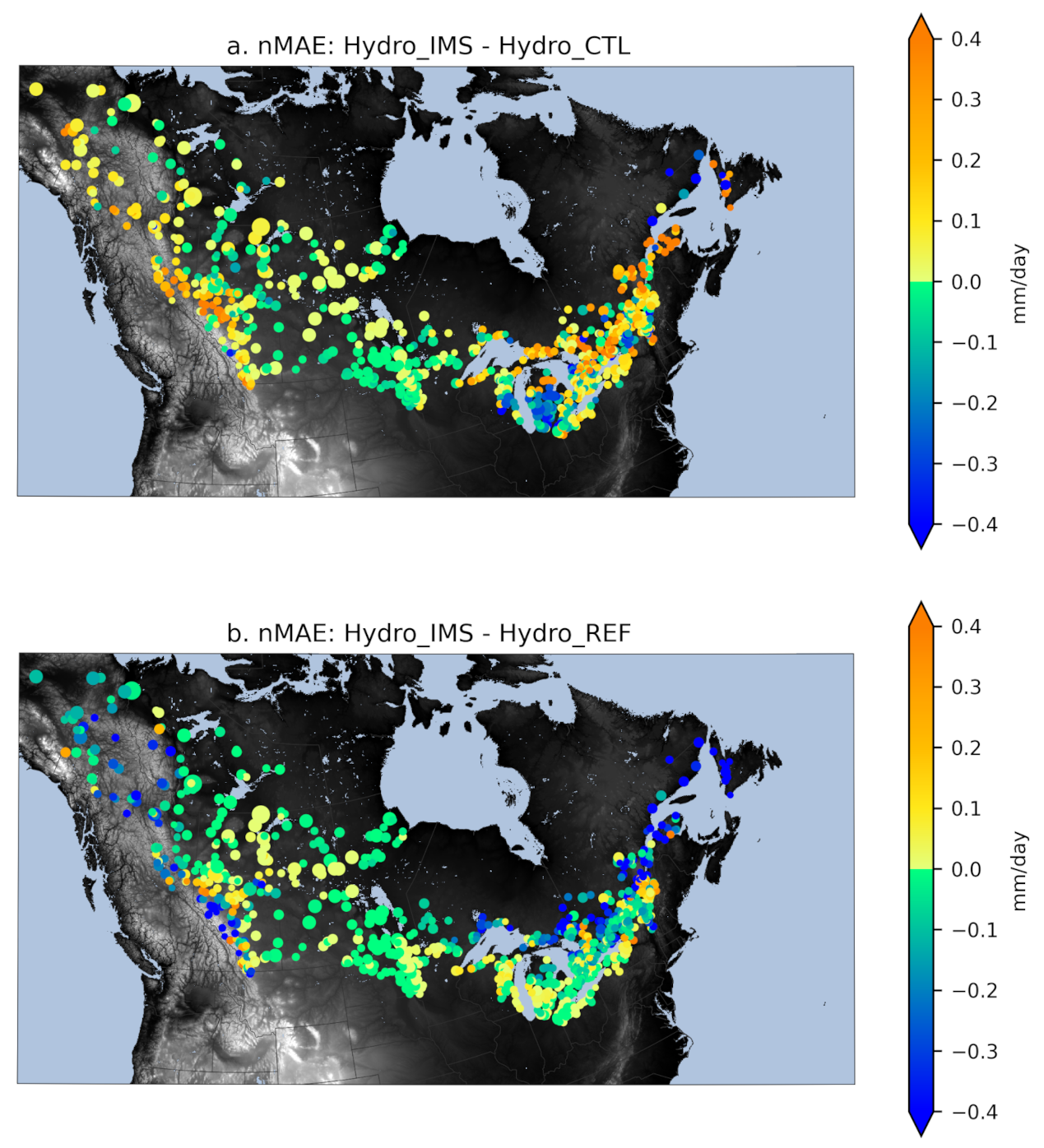
Figure 10) shows that even though all simulations lack water due in part to the precipitation deficit, the enhanced water conservation in CaLDAS_IMS greatly improves streamflow simulations when Hydro_IMS is compared to Hydro_REF, and only slightly degrades the results when compared to Hydro_CTL. A similar result is obtained throughout the study domain with an increase in average MAE of 5.4% compared to Hydro_CTL but a larger reduction of 6.7% compared to Hydro_REF, with the largest improvements along the mountains in the western part of the domain and along St Lawrence river.
In conclusion, this study demonstrates that the new snow data assimilation methodology tested in CaLDAS_IMS brings an overall improvement of snow analyses across the domain, a similar result to what [
16] obtained when assimilating IMS data across the Northern Hemisphere in their Unified Model: improvements in analysed snow cover. In addition, CaLDAS_IMS greatly enhances water conservation compared to CaLDAS_REF, which is reflected in improved streamflow simulations. Compared to what is currently used by the operational DHPS (i.e., outputs from CaLDAS_CTL in wintertime), CaLDAS_IMS has a neutral to positive impact on snowpack simulation, and only slight degradations in water conservation and streamflow forecasts. Since the DHPS is run without discharge data assimilation in this study, streamflow forecasts using CaLDAS_IMS forcing fields will be further improved in an operational NSRPS context where the DHPS is run with data assimilation. The way it is set up, this proposed methodology improves the snow analysis in mountainous regions with the bias correction, in non-mountainous regions where the snow model is constrained by the snow cover extent from IMS through data assimilation, and the resulting enhanced water conservation across the domain, giving us the possibility of using and sharing our snow products throughout the HRDPS domain with increased confidence. ECCC’s hydrologists and environmental modellers are thus confident that the proposed modifications in the snow data assimilation process will be beneficial to ECCC’s clients through the use of improved environmental and hydrological forecasts.
These modifications are, however, only the first step towards a complete update of the snow data assimilation process in CaLDAS. ECCC’s goal is to produce a reliable snow analysis to initialise and improve NWP as well as environmental predictions, including flood and drought forecasts. Future work thus includes testing new assimilation methods, such as a particle filter [
50], to find one that will improve water conservation, as well as increasing the quantity and sources of snow-related observations (SD, SWE, snow cover extent).


 ,
, 


